Dynamic Monitoring of a Mid-Rise Building by Real-Aperture Radar Interferometer: Advantages and Limitations

Abstract

In this paper, remote and in situ techniques to estimate the dynamic response of a building to ambient vibration are reported: data acquired through a real-aperture radar (RAR) interferometer and conventional accelerometers are analyzed. A five-story reinforced concrete housing building, which was damaged during the May 11th 2011 Lorca (Spain) earthquake, is used as a case study. The building was monitored using both types of instruments. The dynamic properties of the building are estimated first taking acceleration measurements using a set of 10 high-precision accelerometers installed on the roof of the building. Further, the displacement–time histories, recorded with the RAR device pointing to a corner of the building, are analyzed. Then, the ability and shortcomings of RAR measurements to deal with the fundamental frequencies of vibration of the structure are investigated. The advantages and limitations of from-inside (accelerometric) and from-outside (RAR) measurements are highlighted and discussed. A relevant conclusion is that, after strong earthquakes, RAR may be an interesting and useful tool, as it allows surveying the structural response of mid-rise buildings remotely, without the need to enter the structures, which may be dangerous for inspectors or technicians in cases of severely damaged buildings. Given that the instrumented building suffered significant damage, the ability of these kinds of measurements to detect damage is also discussed.

1. Introduction

Most guidelines for post-earthquake damage evaluation and traditional damage assessment methodologies rely essentially on expert-conducted on-site visual inspections. Some examples of guidelines developed for different countries are [1,2,3,4,5,6,7]. However, visual inspections are subjective and generally slow in addition to not being feasible for use in severely damaged structures, where the safety of inspectors is compromised. Further, the lack of specialists that are available right after an earthquake requires the participation of non-expert building safety inspectors, which might generate a systematic conservatism due to the lack of experience and personal and safety concerns. As a result, buildings can remain unoccupied for long periods until a final decision regarding their structural safety can be properly made. Any increment of the time between an earthquake and the occupancy allowance of buildings decreases the resilience of cities, thus increasing the need for provisional housing and the loss of services and business opportunities.

Structural health monitoring (SHM) has positioned itself as an objective solution to take rapid post-earthquake decisions regarding structural safety. For this reason, in the past decade, the use of SHM has become a common practice in important buildings and increase the structural safety and to reduce maintenance cost, as well as economic and human loses [8,9]. At the same time, the technological advances of the sensors used for SHM (e.g., accelerometers and displacement or velocity transducers) allow for improvements in the accuracy of the structural monitoring, achieving significant developments in vibration-based damage detection (VBDD). These high-precision sensors have proven to be accurate enough for assessing the dynamic response of structures to strong and weak motions through continuous monitoring [8,10]. However, permanent monitoring requires costly installations and continuous maintenance; hence, this type of monitoring is carried out in a few cases and, generally, in new high-rise buildings, where the owners or the administrations consider it necessary.

In addition, contact devices for SHM must be positioned inside the structure. This can not only be problematic, due to accessibility restriction and installation requirements, but also dangerous after an earthquake. When the structure has symptoms of damage and the risk of collapse as well as likely events such as aftershocks, gas leaks, chemical hazard, exposed electrical wiring and falling non-structural objects is unknown, entrance to the structures should remain restricted. This makes it impossible to install and manipulate any device inside the structure as well as enabling visual inspection. Therefore, the use of non-invasive or remote sensing techniques emerges as a reliable, safer and faster alternative, especially in, but not limited to, post-earthquake scenarios.

In the same way, the idea of punctual or non-continuous monitoring is proposed to evaluate the structure only at specific times, for example, after the construction, in order to identify the dynamic properties in the healthy state, and after a seismic event to estimate whether the structure has been damaged. Remote sensing not only reduces the cost of monitoring significantly, but it can be carried out safely without the need to enter a structure. These advantages are of the utmost importance, so that periodic monitoring can be implemented in a large number of buildings, and this is of great interest to the government as it has a direct impact on the resilience of the cities and the costs involved in the assessment and retrofitting of damaged buildings.

The use of a real-aperture radar (RAR) interferometer is proposed as a good candidate to perform this punctual monitoring. The RAR is a high-sensitivity remote sensing device with a maximum sampling frequency of up to 200 Hz. These types of sensors have exhibited good performance in urban environments under different atmospheric, meteorological and lighting conditions. Noticeably, these devices perform better than other types of contactless sensors, e.g., Laser Doppler devices [11].

However, a potential shortcoming of the RAR technique is that the motion of the soil the RAR system is installed on is combined with the motion of the building, so that the relative motion between the building and the RAR device may be unknown and/or blurred on the recorded signals. Nevertheless, the structural response clearly enhances the modal frequencies of the building, thus making their identification and isolation easy in the RAR recorded signals using advanced methods for signal analysis—narrow band pass Butterworth filtering, in our case. This issue would be particularly relevant if measurements were taken during strong ground motion due to great earthquakes, since the device’s base is not fixed, and the ground motion would be important. Considering these effects, up-to-date RAR devices incorporate an accelerometer, allowing RAR operators to properly address this issue. In any case, the RAR device used in the case study shown in this article may not be suitable for use during great earthquakes. As this method is also intended to be used after damaging earthquakes, in these cases, people with responsibilities for emergency management, usually including firemen, civil protection personnel and other authorities, should identify buildings that require study and suggest proper locations that are stable, safe and proper for the easy and fast installation of the equipment in front of the buildings/structures to be surveyed.

The use of the RAR to determine the dynamic properties of buildings is a present and actual issue [12,13]. Remote RAR measurements have been widely and successfully used for monitoring large civil structures including bridges and towers [14,15,16,17,18], wind turbines [19,20], chimneys [21,22,23,24], and heritage and high-rise buildings [25,26,27,28]. However, combined accelerometric- and RAR-based applications to damaged low- and mid-rise conventional buildings are not so frequent nor so successful, mainly because of the low periods (high frequencies) and very low displacements involved, which may compromise the ability of techniques based on RAR technology to help in these cases. In this article, both methods are applied to a mid-rise building that was severely damaged during an actual earthquake, providing insight into the ability of RAR to properly address these kinds of problems. Extending the use of RAR to mid-rise buildings is of great importance, not only because this typology of buildings represents a large amount of the structures built in the world but also because it is among the most vulnerable structures in seismic scenarios.

The signal analysis techniques often used to analyze the acceleration and displacement–time histories are the power spectral density (PSD), periodogram, and peak picking method (PPM). In this article, other methods such as the cross power spectral density (CPSD) and the magnitude-squared coherence (MSC) are investigated. These advanced methods may help to overcome issues from high noise amplitudes compared to the very low amplitudes of the building displacements, significantly improving the resolution and the quality of the obtained results.

Finally, joint synchronous analyses of the acceleration–time histories will allow us to identify not only the main modal frequencies but also the type of motion involved, which, in our case, are rotation and translation, respectively, for the first and second modes of vibration. In addition, the joint analysis of the synchronous displacement–time histories of the Rbins, corresponding to microwaves reflected at different heights of the building, will indicate the ability of RAR measurements dealing with the corresponding modal shape.

In this study, the use of RAR for the identification of fundamental frequencies in a building that suffered severe damage during the May 11th 2011 earthquake is analyzed and discussed. To this end, first, the dynamic response to ambient vibrations of this building has been evaluated through a network of ten high-precision axial accelerometers. Time–frequency domain analysis is used to identify the natural frequencies and modal shapes of the building. These results are compared with those obtained from remote monitoring through RAR.

To improve the modal property recognition with RAR, the capability of this device to simultaneously measure different parts of the building [14,25,29,30] is studied. In addition, in the processing of the displacement samples with respect to more classical methods, such as the power spectral density and periodograms, the use of other signal analysis methods, in the frequency domain, is proposed. In particular, methods based on the CPSD and the MSC that allow us to search for common frequency contents of signals with high levels of noise [31,32,33,34,35]. All calculations of these analyses were made with programs developed in MATLAB® [36] software. Figure 1 shows a scheme of the research methodology. A detailed description of each module is given in the following section, devoted to the methodology and to its application to a case study.

Finally, based on the analyzed experimental results, the main advantages and limitations of the use of RAR to characterize the dynamic properties of conventional buildings are discussed. Other issues related to the frequency domain analyses of the obtained displacement–time histories are also presented. The potential of this device to detect structural damage, by comparing the fundamental period of structures in their undamaged and damaged state, is also discussed.

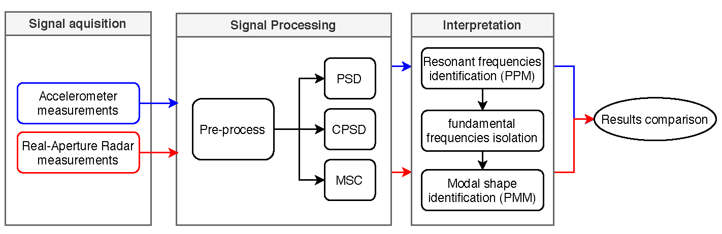
2. Materials and Methods

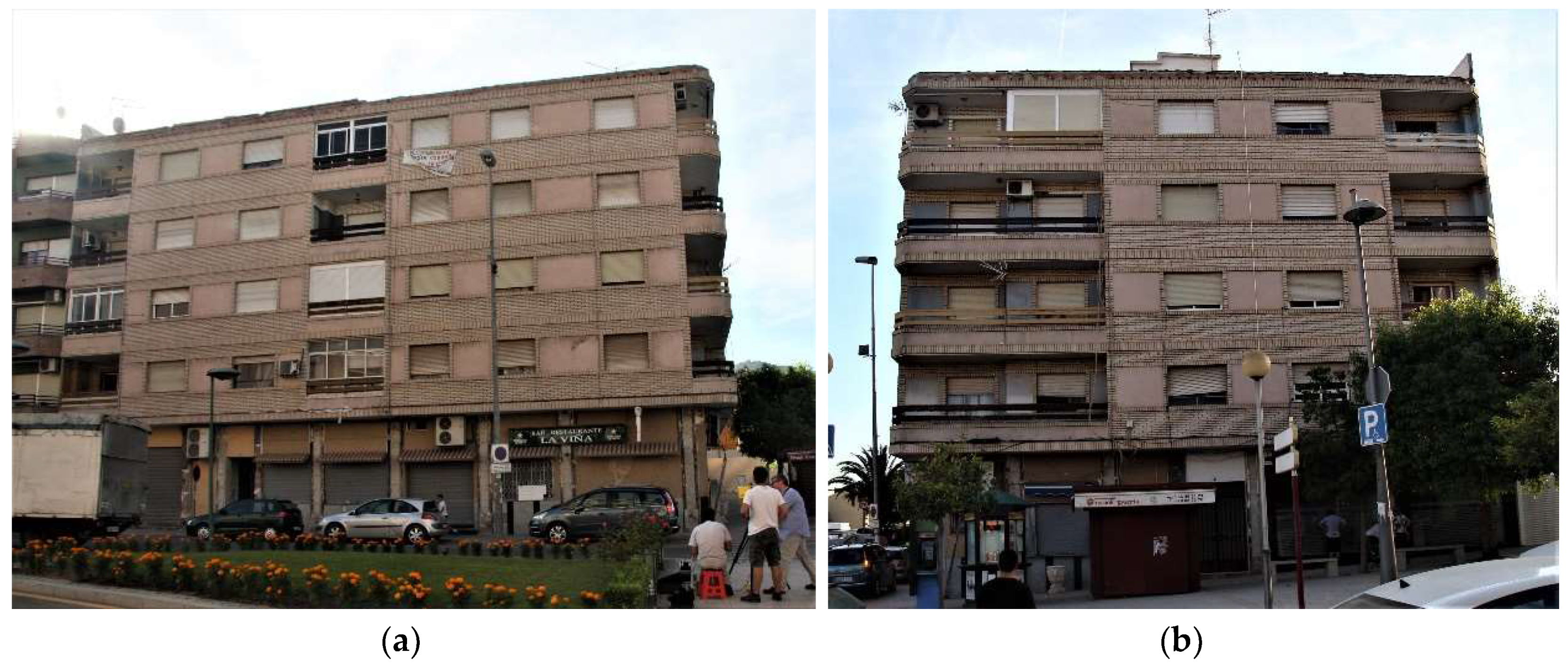
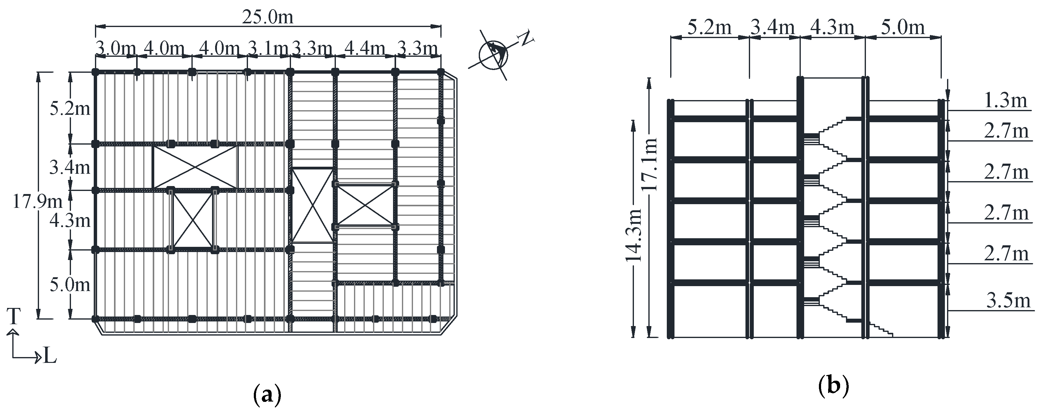
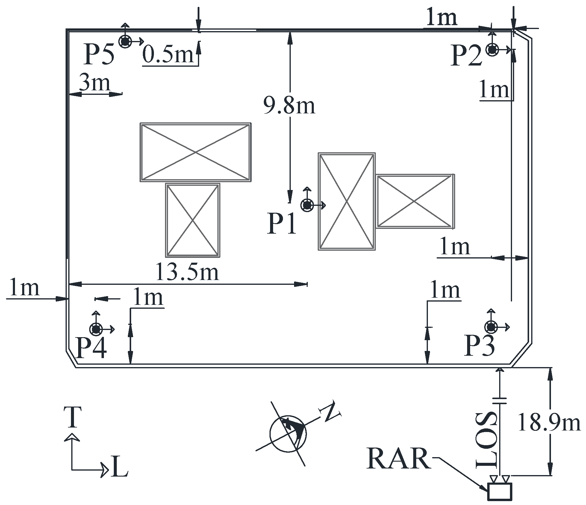
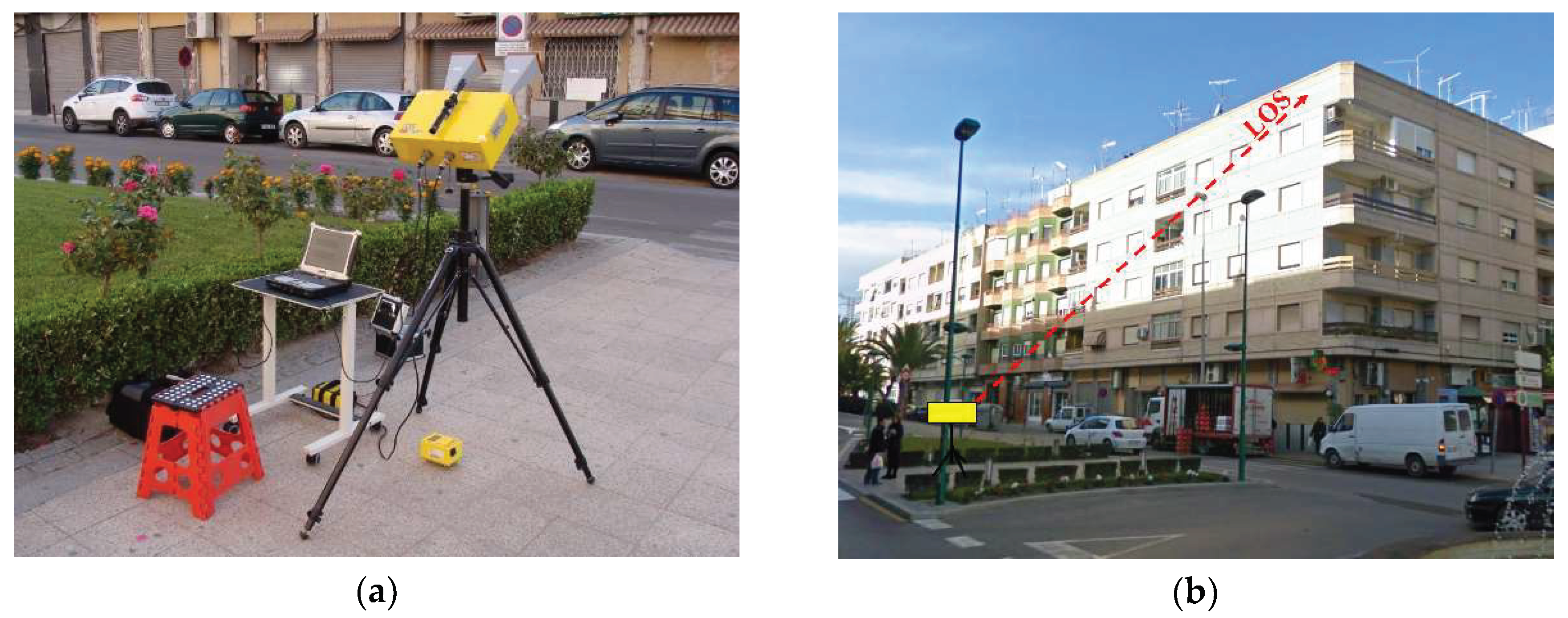
2.1. Case Study

The studied structure is a five-story reinforced concrete (RC) building with masonry infill walls, damaged during the May 11th 2011 Lorca earthquake ($M_W=5.2$). The building has a constructed area of 2408 m² and consists of a ground floor for commercial use and four floors with 16 apartments. The longitudinal axis (L) of the surveyed building has an orientation of N 28°E and its transversal (T) axis is orientated N 62°W. The floor plan dimensions are 17.9 m in width by 25.0 m plus a 1 m cantilever in both directions in the upper floors. The height of each story on the first floor is 3.5 m, and 2.7 m for the upper floors. The total height of the building is 17.1 m. Figure 2 and Figure 3 show the L and T façades and the geometry of the “La Viña” building, respectively.

2.2. Accelerometer Instrumentation

Acceleration–time histories of the response of the building to ambient vibration were simultaneously recorded at five sites on the roof of the building: at a central point (P1) and at the four corners, north (P2), east (P3), south (P4), and west (P5). These locations were chosen in order to capture the first modes of vibration of the structure. At each point, one high-sensitivity accelerometer (Brüel and Kjær 8340) was placed for each direction, giving a total of ten accelerometers measuring simultaneously. The measurements in the longitudinal direction (L) of the building correspond to the orientation N 28°E, while the measurements in the transversal direction (T) coincide with the orientation N 62°W. The arrangement and location of the sensors are shown in Figure 4.

Acceleration data were recorded, continuously and synchronously, for 25 min at each of the five points on the roof. A sampling frequency of 200 Hz was set for the acceleration records. Baseline correction was performed, and a Butterworth band-pass filter was applied in the frequency range of interest (1–5 Hz). Figure 5 shows six-second sections (0.1 min) of the ten processed signals.

Natural Frequencies: The Accelerometric Technique

In order to detect the natural frequencies of a structure, the frequency of the recorded vibration was investigated using the power spectral density (PSD); the Welch method [37] has been used in this case. The signal analysis on the frequency range was focused between 1 and 5 Hz (periods between 0.2 and 1 s); for this, a band-pass Butterworth filter was applied to the measured displacement–time and acceleration–time histories. The natural frequencies that appear as peaks in the PSD can be picked in an easy way. This frequency domain method, also known as the peak picking method (PPM) [38,39], has been extensively used for its simplicity, showing good results, especially for finding the frequencies of the first modes of vibration.

Table 1. The first three peaks in order of increasing frequencies, picked in the L and T directions.

Direction	1		2		3
	f (Hz)	T (s)	f (Hz)	T (s)	f (Hz)	T (s)
L	2.49	0.40	2.79	0.36	3.98	0.25
T	2.49	0.40	2.79	0.36	3.98	0.25

shows the PSDs for the ten channels. Peaks with similar spectral shapes can be observed in all channels. The first two peaks of approximately 2.49 and 2.79 Hz are clearly identified in both the T and L directions. The presence of the same resonant frequencies in both directions may indicate the existence of flexural–torsional modes. A third peak, minor in most of the channels, is found at a frequency of 3.98 Hz. Figure 6 shows the three frequency peak values with the highest PSD. At this point, it is difficult to assign these values to the modes of vibration of the building.

2.3. The Real-Aperture Radar (RAR)

The RAR used in this study was designed by the Italian company IDS (Ingegneria dei Sistemi SpA). The device is portable and is mounted on a tripod, allowing the rotation and tilt to easily point towards the target structure (see Figure 7). This system consists of a sensor, a coherent radar, connected to a portable computer through Universal Serial Bus (USB) and powered by an external battery that allows up to 5 h of continuous use. The sampling parameters can be adjusted with the provided software. More details on the use and specifications of the RAR used in this study can be found in [13,14].

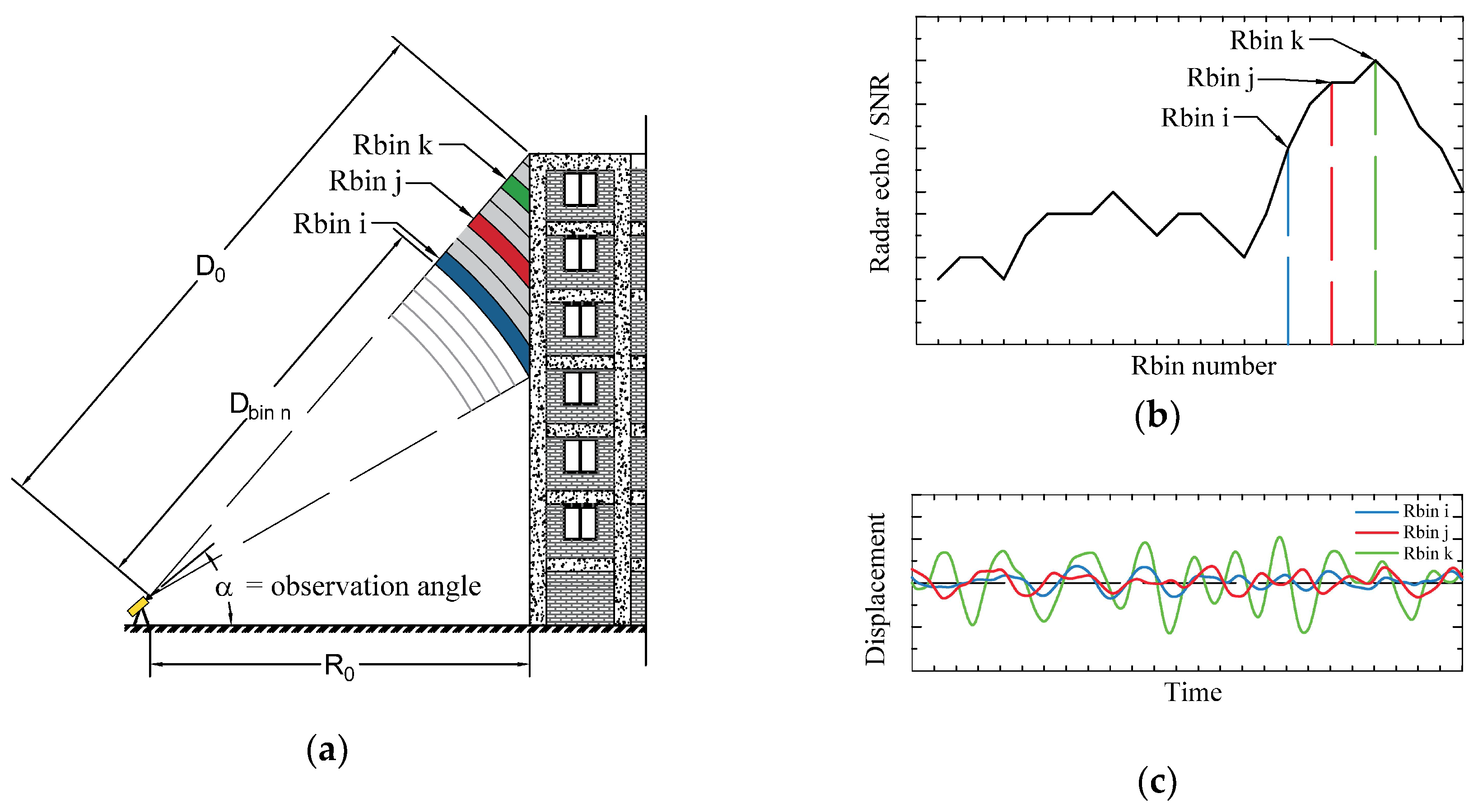
2.3.1. RAR Interferometry

The RAR measures displacements by interferometry. The principle entails the measurement of the phase difference between the transmitted microwave signals and signals back reflected from the moving target building. Then, the radial displacement in the line of sight (LOS) of the RAR is calculated according to Equation (1).

$$d=\frac{\lambda }{4\pi }\left({\phi }_2-{\phi }_1\right)$$

(1)

where $\lambda$ is the wavelength and ${\phi }_1$ and ${\phi }_2$ are the phases acquired at the different times. The expected precision is in the order of tens of micrometers, when good phase stability is achieved with high SNR. A detailed description of the working principle of the RAR can be found in [13,14].

One main feature of the radar is that it can simultaneously capture the movement of different objects that are in the field of view (FOV) of the RAR antenna. Objects separated from each other by more than 0.5 m can be captured in different so-called Range bins (Rbin) [14]. In the case of buildings, the radar allows recording the displacement at different heights of the building, depending on the height of the building and on the measuring distance. However, the vibration of non-structural objects on the facades and any other objects in the FOV of the RAR can also be captured. Therefore, the interpretation of the time histories corresponding to each Rbin must be performed carefully. It is necessary to bear in mind that: (a) the structure must be spatially located within the range profile in order to select and study only the bins containing the structure displacement and, (b) the building displacement signal must be distinguished from the noise produced by non-structural elements and other objects within the RAR LOS.

In order to help in this careful interpretation, the range profile expresses the quality of the received signals, in terms of SNR, as a function of the Rbin number. In this case, high SNR peaks, within the bins corresponding to the structure, indicate that the time history recorded corresponds well to the displacement of the building. Thus, the range profile is very useful in locating Rbins that more likely correspond to the true displacement of the structure.

Figure 8 depicts a scheme of a typical RAR measurement: (a) the radar sends and back receives the signal from different parts of the building in different Rbins located at a distance $D_{bin}$; (b) the amplitude of the radar echoes according to the different Rbins is plotted into a range profile in terms of SNR, allowing Rbin selection according to the range of the structure and the SNR; and (c) the interferometric phase of the selected Rbins is converted to a displacement–time recording using Equation (1) [25].

It is required to record a displacement history long enough to obtain sufficient frequency resolution that allows investigating the buildings harmonics. In addition, filtering the signal also serves to set aside the vibration frequencies of objects that are not within the range of interest. Although the above precautions may be sufficient for high-rise buildings with long periods/very low frequencies, in the case of mid- and low-rise buildings with short periods/high frequencies, as discussed later in this article, the resonant frequency estimation by these traditional frequency domain techniques can be a difficult task. Therefore, it is necessary to explore different techniques for signal analysis. Several techniques such as multiple coherence are discussed below.

2.3.2. In-Field RAR Remote Monitoring

For the purpose of this research, only the displacement on the east corner of the building, which corresponds to the transversal direction, was measured. To remotely monitor the structure, the RAR system was positioned on the other side of the south-eastern street at a distance of $R_0=18.9 m$ ($D_0=25 m)$ from the base of the structure. $R_0$ and $D_0$ were as defined in Figure 8. The inclination angle was $\alpha =41°$ above the horizontal. The RAR antennas were pointed to the upper part of the building (see Figure 7 and Figure 8). The measurements lasted 36 min, with an output sampling frequency of 149 Hz.

Figure 9 shows the Range bin profile of the RAR campaign of the “La Viña” building. According to the distances to the building, it was estimated that the bins Rbin38, Rbin39, Rbin40, Rbin41, Rbin42 and Rbin43 contain information on the structure. It can also be observed that the SNRs are the highest among the selected Rbins recorded.

Once the structure is located within the range profile, we obtain the time history of displacements corresponding to the selected Rbins. Figure 10a shows the as-recorded signals of the five selected Rbins; Figure 10b displays a six-second (0.1 min) fragment. As part of the signal processing, the baseline was corrected. Vibrations outside the range of frequencies of interest were removed using a band-pass Butterworth filter. Figure 10c shows the processed signals. Finally, Figure 10d shows a six-second fragment.

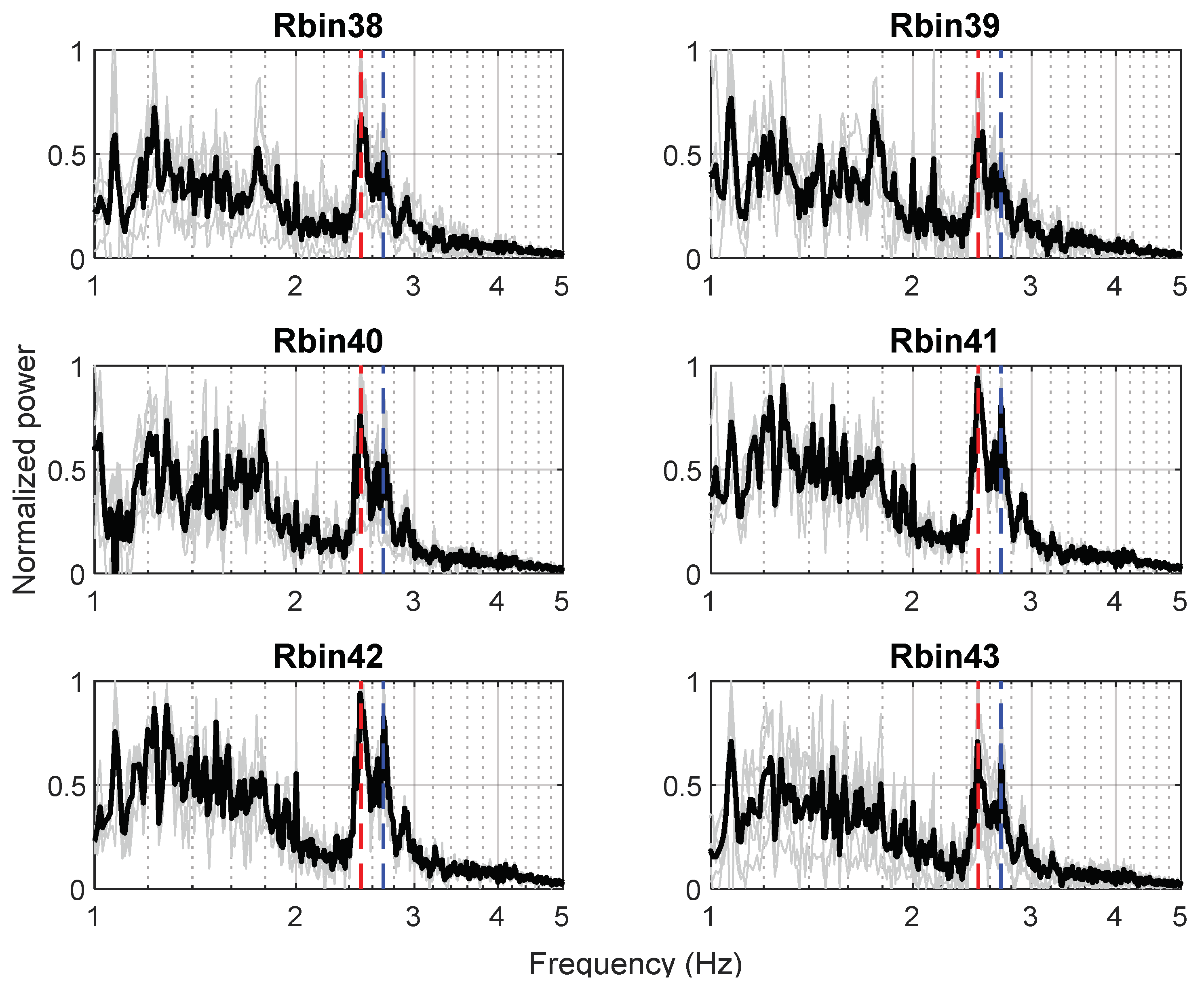
2.3.3. Natural Frequencies: The RAR Technique

To investigate the feasibility to find resonant frequencies using the PPM, the PSDs were calculated for each Rbin (Figure 11). To do this, a Hamming window with 50% overlap was used. As can be seen, there are no clear outstanding peaks in the PSDs of the selected Rbins that could indicate resonant frequencies as they have been straightforwardly found using accelerometers and the PPM. Although the Rbins shown are those with a higher SNR, the same peaks are not present in all the different bins and are not clear outstanding peaks. Rbin41 and Rbin42, however, present clearer peaks near the frequencies identified with the accelerometers, indicated with blue and red dashed lines in Figure 11, and they have similar PSDs. This may be due to the greater precision that can be obtained with these Rbins since they are the ones with the highest SNR. Note that Rbin 41 and Rbin 42 are in the highest peak of the Range bin profile of Figure 9, corresponding to the highest SNR.

2.4. Other Techniques for Resonant Frequencies Identification

Because of difficulties using RAR in rigid structures, other signal analysis tools based on the similarity/dissimilarity of the recorded signals using the correlation have been utilized in this work.

This way, the linear correlation between the signals of the selected Rbins has been calculated using the Pearson linear correlation coefficient (PLCC) [40]. The PLCC is a statistical quantity that estimates pairwise linear correlation between two signals. The coefficient ranges from −1 to 1, indicating negative and positive total correlation, respectively, and 0 indicates no correlation at all.

Figure 12 shows the PLCC correlation matrix, where it is observed that all the signals show positive correlation. Only the Rbin41 and Rbin42 are highly correlated, with a PLCC of approximately 95%, as can be intuited from Figure 11, where the similarity of the PSDs is shown. Among the other Rbins, the correlation is relatively low. We can attribute the high correlation to the displacement of the building with a higher SNR recorded by both bins.

With the above, we have focused on the Rbin41 and Rbin42 to analyze their frequency content in a narrower band (Figure 13). As mentioned before, we can appreciate that the main peaks correspond to frequencies of 2.49 and 2.71 Hz, similar to those frequencies identified with the accelerometric network, and which more likely correspond to the first and second mode of the structure. However, only analyzing the PSDs does not make clear whether these frequency bands correspond to the resonant frequencies of the building. In addition, the third resonant frequency of 3.98 Hz, identified with the accelerometric network, is not present in the PSDs of the RAR Rbin signals.

Thus far, we have focused on data recorded from each Rbin and tried to obtain features of the dynamical properties of the structure based on separately studying the outputs. However, the RAR allows synchronously measuring different points of the structure. This advantage is studied by two different multisignal analysis methods: the cross-power spectral density and the magnitude-squared coherence.

2.4.1. Cross-Spectrum Method

The cross-power spectral density (CPSD) is used to determine the similarity or relationship of the linear dynamic properties, between two different time series, as a function of frequency. This technique is especially useful when a high level of noise is present in the signals and it is not possible to find significant peaks in the power spectra that allow indicating the related periodicities among the signals. Because ambient noise can be considered as random Gaussian noise, there should not be correlation between the noise and the harmonics corresponding to the movement of the building. This is the case with the measured radar signals and only the shared harmonics between the signals will be present in the CPSD.

To estimate the CPSD, the averaged Welch [37] method can be used. To do so, we first divide the signals $x$ and $y$ in $K$ overlapped and windowed segments of length $(L$). Then, we compute the Fourier Transform of the respective pair of segments, $x^i$ and $y^i$, via Discrete Fourier Transform (DFT) as follows:

$$P_{xy}^i\left(f\right)=\frac{1}{L}{\displaystyle \sum }_{k=0}^{L-1}{X}^i\left(f\right)Y^{i \ast }\left(f\right),n=0,1\dots .,L-1$$

(2)

where $X^i\left(f\right)$ and $Y^{i \ast }\left(f\right)$ are the DFTs of the respective windowed segments and the superscript asterisk denotes the complex conjugate. Finally, we compute the CPSD, as in the Welch method, as follows

$$\overline{P_x}\left(f\right)=\frac{1}{K}{\displaystyle \sum }_{i=1}^K{P}_{xy}^i\left(f\right)$$

(3)

Figure 14 shows the CPSDs of the combinations between P3 and the other four points, in the same direction, for both L (a) and T (b) directions, i.e., between P3-L and P1-L, P2-L, P4-L and P5-L. The mean CPSD is highlighted in black. It can be seen that peaks in the frequencies of 2.487 and 2.786 Hz, indicated with dashed red and blue lines, respectively, are emphasized while the other peaks tend to attenuate.

Similar results can be seen with the RAR signals. In Figure 15, the CPSD estimates for the RAR measurements are presented. The CPSDs for all combinations between the selected Rbin and the rest of the Rbins are shown in grey, i.e., for Rbin38, the CPSDs between Rbin38 and Rbin39, Rbin38 and Rbin40, Rbin38 and Rbin41, Rbin38 and Rbin42 and Rbin38 and Rbin43 are plotted together in grey. Finally, the mean value of the CPSD combinations is highlighted in black. The peaks at the resonant frequencies of 2.491 and 2.708 Hz clearly stand out. The peaks of different frequencies in the range from 1 to 2 Hz are also visible in most of the CPSDs. However, these peaks are outside the frequency range of interest for this building and do not appear to be stable in all the CPSDs.

2.4.2. Magnitude-Squared Coherence Method

The magnitude-squared coherence (MSC) indicates the correlation of two signals at a certain frequency. The MSC is 1 when there is complete similarity in the spectral content at a given frequency and 0 when the signals are fully uncorrelated in that frequency band. One major advantage of the MSC is that a different amplitude in harmonics does not affect the MSC between the signals. In addition, the MSC is phase independent. This is important for analyzing superior modes of vibration, where two or more levels of the structure vibrate with the same harmonics but with different phases. However, external sources of vibration that were detected at the different measurement points may cause high MSCs at the frequencies of the origin of vibration. This happens for example when the structure is excited with some device (reference) or with different types of machinery working, i.e., air conditioning systems. In the case of the building under study, there was no source of noise and the structure was evicted so that ambient noise was the only source of excitation of the structure.

The coherence spectrum is analogous to the conventional correlation coefficient and is defined as follows:

$$C_{x,y}\left(f\right)=\frac{{\left|P_{x,y}\left(f\right)\right|}^2}{P_x\left(f\right)P_y\left(f\right)}$$

(4)

where $P_x\left(f\right)$ and $P_y\left(f\right)$ are the power spectral densities, and $P_{xy}\left(f\right)$ is the cross-power spectral density between the signals $x$ and $y$. In other words, the coherence is a statistical indicator which specifies whether or not two signals are correlated. For cases in which the correlation degree between a selected signal $s$ and a group of signals $Z=\left\{z_1,z_2,\dots ,z_n\right\}$ is to be estimated, the Multiple Magnitude Coherence Method (MMSC) [33] can be used. The multiple coherence is defined as:

$$\begin{array}{c}{M}_{Zs}\left(f\right)=\frac{P_{Zs}^{\ast }\left(f\right)P_{ZZ}^{-1}\left(f\right)P_{Zs}\left(f\right)}{P_s\left(f\right)}\\ =\left[\begin{array}{ccc}{P}_{z_1{s}_i}^{\ast }\left(f\right)& \cdots & P_{z_n{s}_i}^{\ast }\left(f\right)\end{array}\right]\left[\begin{array}{ccc}{P}_{z_1{z}_1}& \cdots & P_{z_1{z}_n}\\ ⋮& \ddots & ⋮\\ P_{z_n{z}_1}& \cdots & P_{z_n{z}_n}\end{array}\right]\left[\begin{array}{c}{P}_{z_1{s}_i}\\ ⋮\\ P_{z_n{s}_i}\end{array}\right]\frac{1}{P_{s_i}\left(f\right)}\end{array}$$

(5)

where $M_{Zs}\left(f\right)$ is the multiple coherence function between the signal $s$ and the array of signals $Z$, $P_{Zs}\left(f\right)$ is the $n$-dimensional vector of the cross-power spectral densities between the signal $s$ and the series of signals $Z$, $P_{ZZ}^{-1}\left(f\right)$ is the inverse matrix of $n x n$ dimension of the PSD and the CPSD of the series of signals $Z$ and $P_s\left(f\right)$ is the PSD of the signal $s$.

Figure 16 shows the MSC estimate for point 3 as an example. The gray lines represent the MSC of the different combinations between the selected channel and the other channels for the same direction—that is, between P3-L and P1-L, P2-L, P4-L and P5-L for the longitudinal direction (Figure 16a) and between P3-L and P1-L, P2-L, P4-L and P5-L for the transversal direction (Figure 16b). The mean spectra of the MSC is shown in black. It can be observed that, as in the CPSDs, there are predominant peaks in the frequencies corresponding to 2.49 and 2.79 Hz, highlighted with dashed red and blue lines, respectively.

Figure 17 shows the MSC between the combinations of Rbin and the rest of the selected Rbins (grey lines), i.e., between Rbin41 and Rbin38, Rbin39, Rbin40, Rbin42 and Rbin43, and the mean MSC is shown in black. It can be observed that the highest MSC peaks are present in frequencies 2.49 and 2.71 Hz. The same frequencies are found in the peaks of both the PSD of Rbin41 and Rbin42 and in the mean cross-spectrum peaks. It can also be seen that the lower frequency peaks, between 1 and 2 Hz, are attenuated. Remarkably, the resonant frequencies identified with the CPSD and the MMSC are virtually the same as those found with the traditional techniques using accelerometers.

3. Results

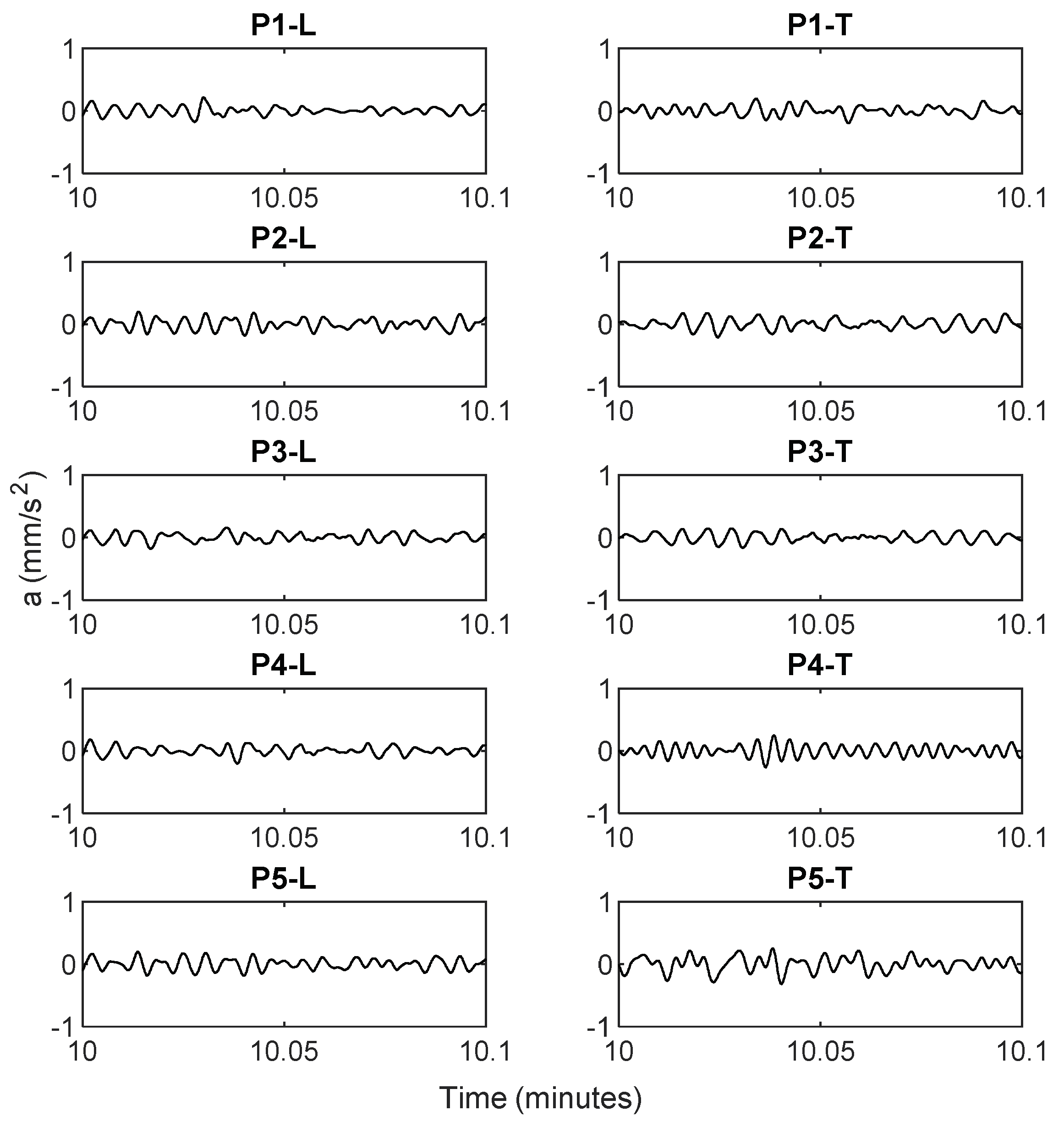
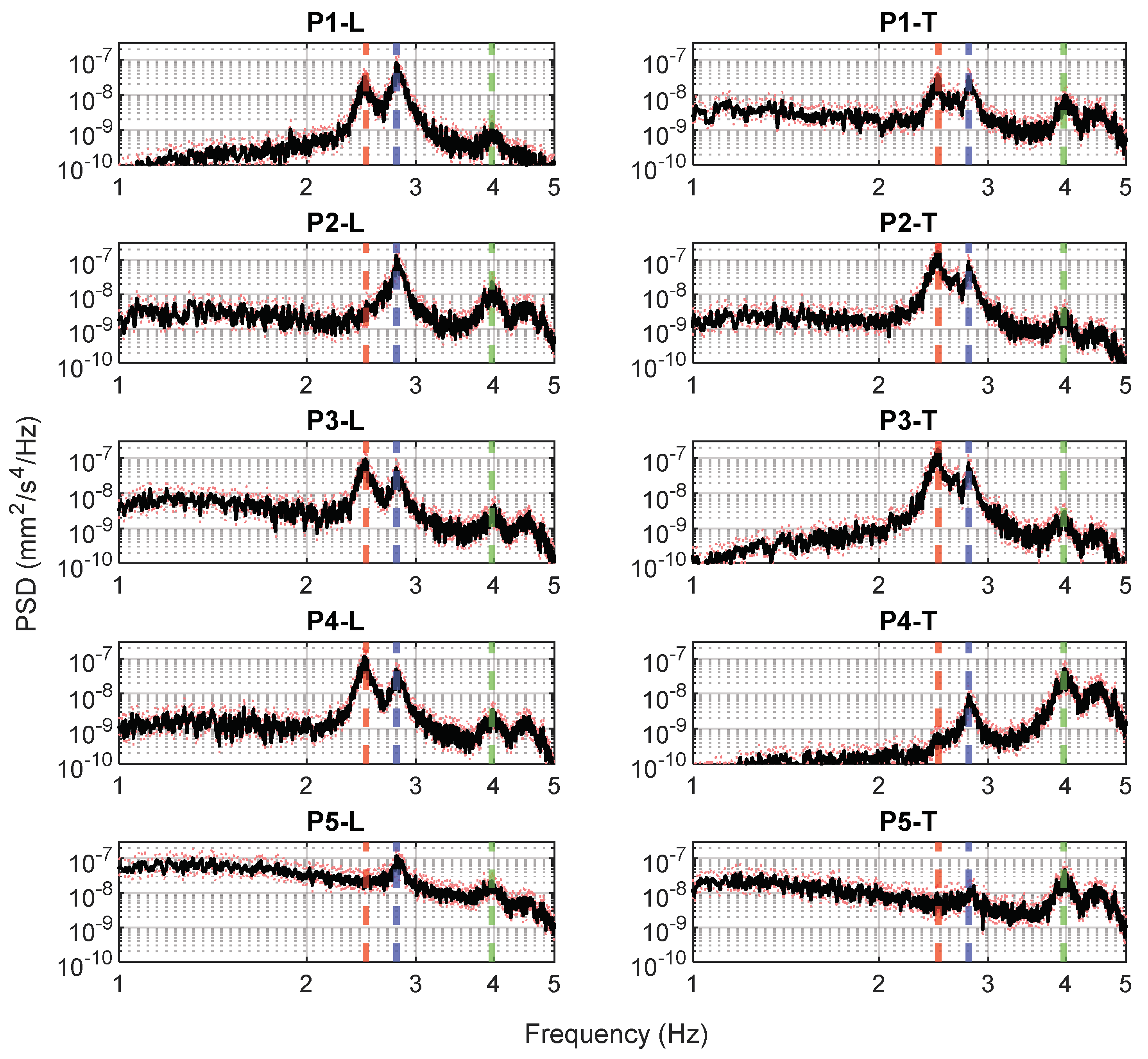
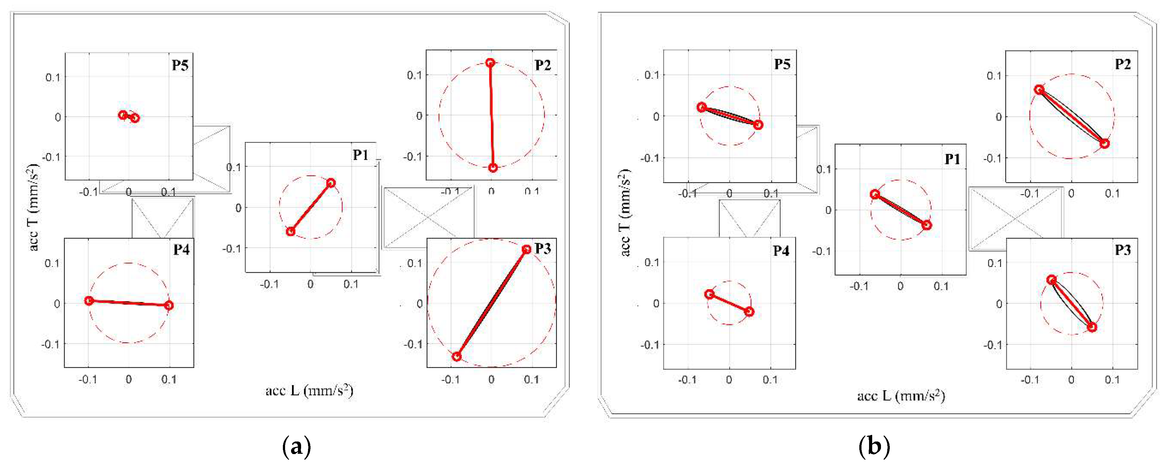
3.1. Modal Identification by Accelerometer Array

The first two modal shapes at each measurement point are recognized by the particle movement technique [41] using accelerometer array. This technique requires filtering the signals on a narrow (e.g., 0.01 Hz) band-pass and setting the identified resonant frequencies as the center of the band-pass. For this purpose, a Butterworth band-pass filter was used. The width of the band-pass was sufficiently narrow to prevent nearby frequencies from contaminating the analyzed natural frequencies.

The modal shape for the first resonant frequency of 2.49 Hz was estimated for each of the measured points. For this, a third-order Butterworth band-pass filter was applied in all the channels between frequencies 2.485 and 2.495 Hz. Figure 18a shows the particle movement of the acceleration signals in both directions for each of the points.

The mode corresponding to the aforementioned frequency is torsional, generating greater accelerations along the T-axis of the N–W façade, corresponding to the axis of the more flexible direction of the structure. The rotational mode can explain the presence of the same resonant frequencies in the PSD of the signals in both directions. It can also be observed that point P5 has the lower accelerations in this frequency range. This fact could be due to the possible coupling with another building on the S–W façade, or superior stiffness in the S–W and N–W façades due to the absence of windows and openings.

For the second frequency identified, the acceleration component corresponding to the frequency of 2.79 Hz was isolated using a band-pass filter between the cutoff frequencies of 2.785 and 2.795 Hz. In Figure 18b, the acceleration particle motion results for each of the five points measured on the roof of the studied building are shown. It can be observed that this frequency relates to a combined translational mode between both the L and T directions. The amplitude of the acceleration for this mode is similar in the five measured points of the structure and follows an E–W direction.

The modal shapes are described in Figure 19, where the first and second modes of the building are depicted. The first mode (Figure 19a), corresponding to a frequency of 2.49 Hz, is mainly rotational and the second mode (Figure 19b) is a combined translation mode with a frequency of 2.79 Hz.

Finally, in order to find the fundamental frequencies and modes of the structure, it was necessary not only to find the highest energy peaks of the PSD by applying the widely used PPM, but also to isolate and study the dynamics corresponding to each of the selected frequencies. This is required to find out whether the natural frequencies correspond to the structure motion and not to an isolated or external element, inducing high-energy peaks in the PSD. In fact, the isolation of these two frequencies for all of the acceleration sensors allows us to depict the particle motions corresponding to each frequency (Figure 18) at different sites of the structure, which, in this case, are located on the roof. This allows us to link the recorded motion and the vibration modes. The first frequency clearly corresponds to a rotation mode, while the second frequency corresponds to a translation mode. The results of the first two frequencies and modes, corresponding to the studied building, are shown in

Table 2. Modal results of the “La Viña” building.

Mode	Type	f (Hz)	T (s)
1	Rotational	2.49	0.40
2	Combined translational	2.79	0.36

.

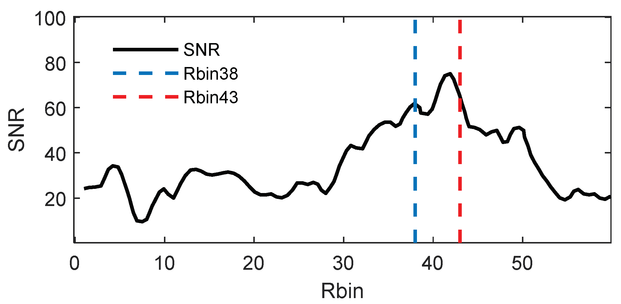
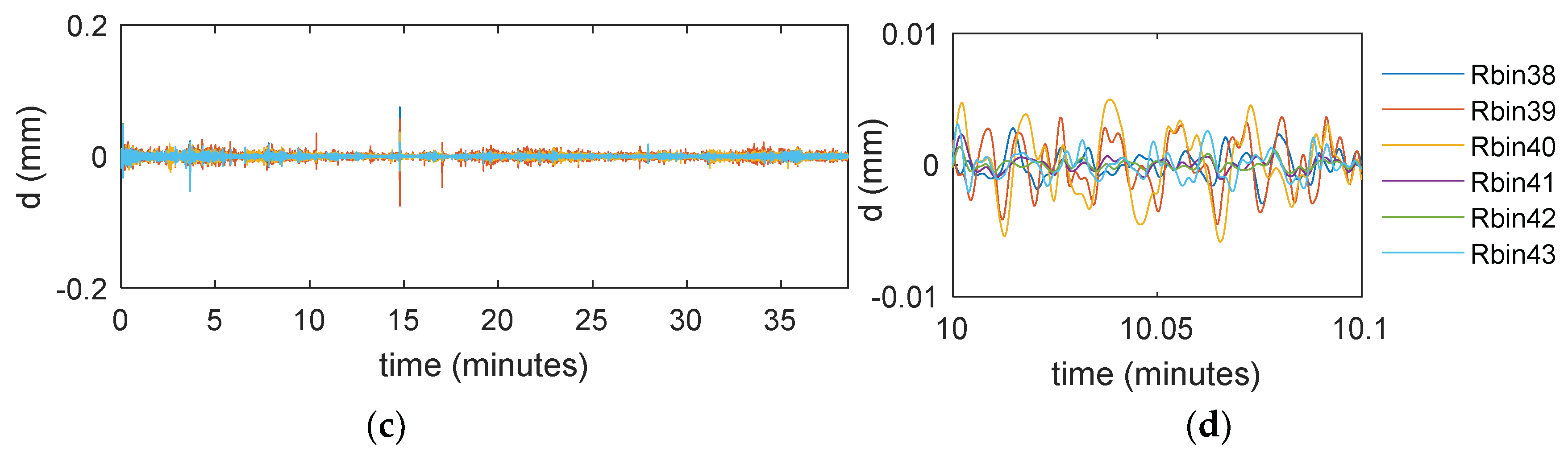
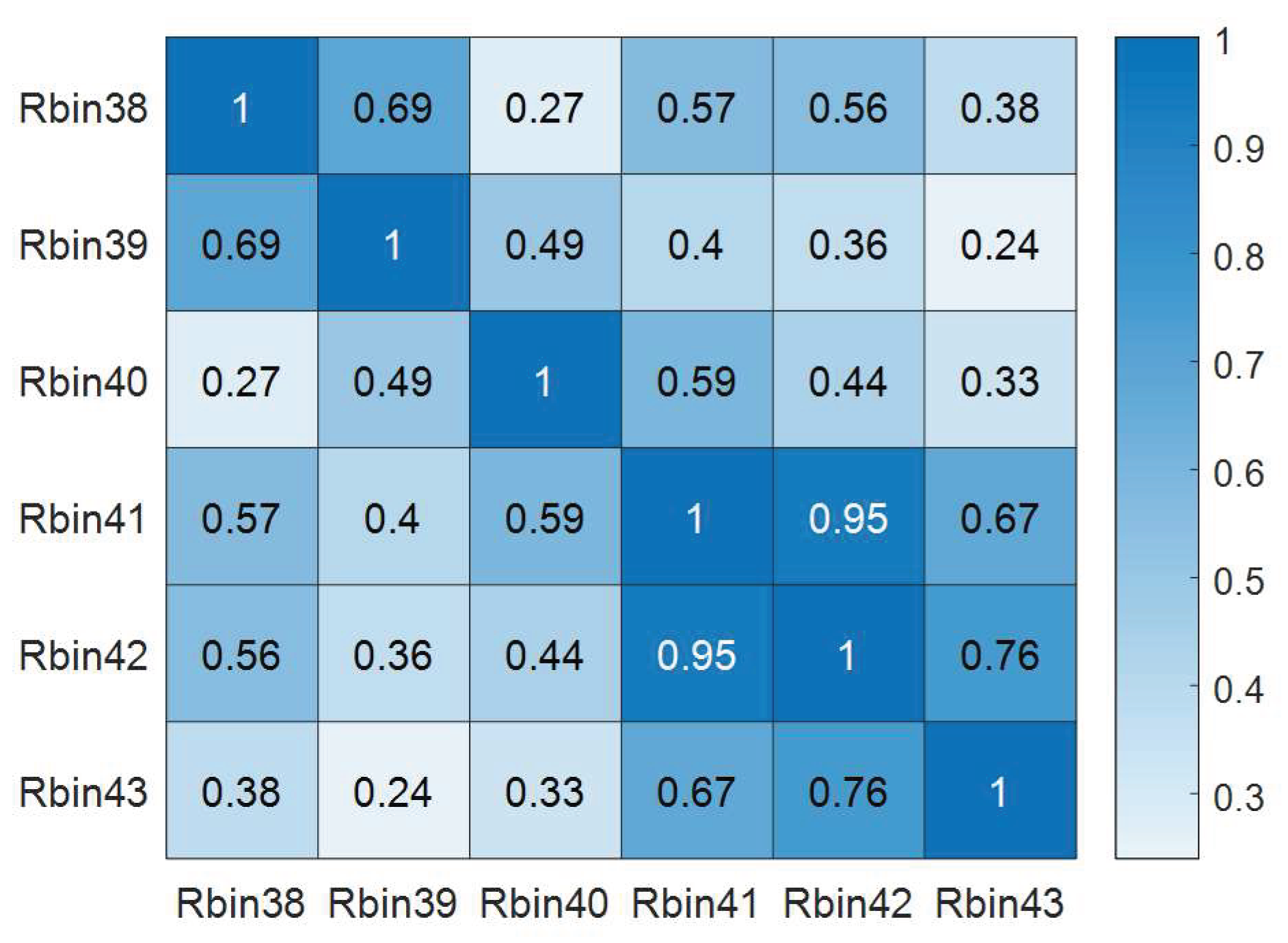
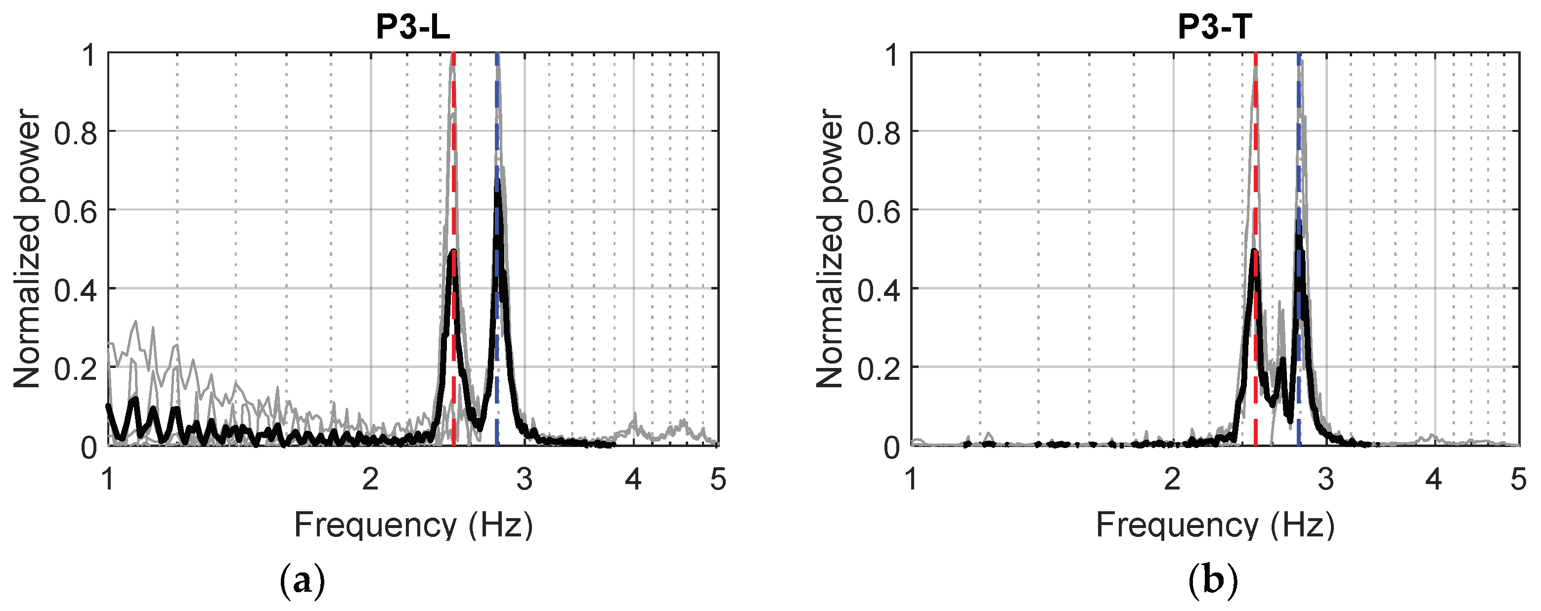
3.2. Modal Identification by RAR

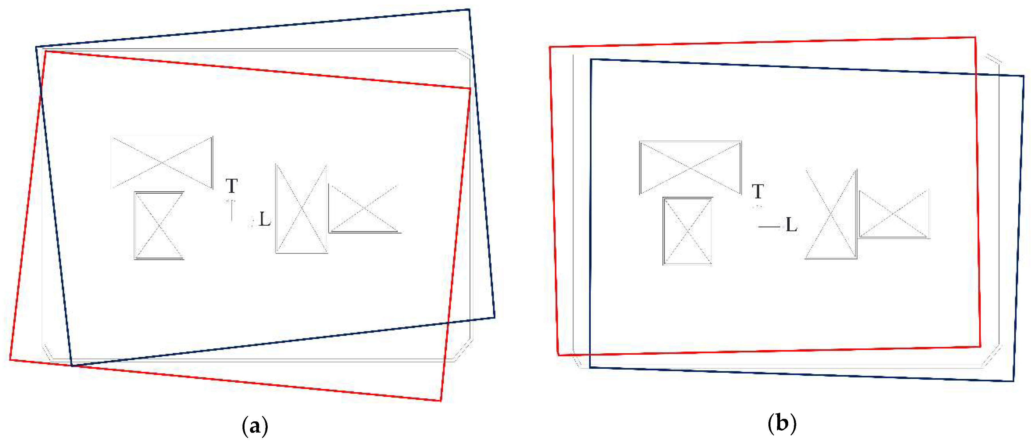
Recent advances in remote sensing techniques confirm the possibility of extract the modal shapes with the use of RAR in high-rise buildings [28]. The greater displacements shown by these types of structures simplify the extraction. To investigate the possibility of estimating the modal shapes of the studied structure using RAR, the following assumptions were considered: (1) the RAR measures the movement of the structure at different elevations on each Rbin, (see Figure 8a); (2) the motion recorded from the different Rbins is synchronized and (3) the relative displacement between the RAR and the base of the structure is negligible.

Figure 20a shows a cycle of 0.4 s (from 60.25 to 60.65 s) from the history of the displacement measured by each of the bins for a frequency of 2.49 Hz, corresponding to the first identified mode of the “La Viña” building. For this, a Butterworth band pass filter was used between 2.490 and 2.492 Hz. The five different time instants are represented by the circles. Figure 20b shows the five displacement instants of each of the bins. The movement of the base has been set to zero. Due to the resolution of the Rbins of the RAR, it is difficult to assign a measurement point to each of the Rbins, and so the vertical axis is not exactly related to the height of the building. It can be seen that the motion is similar at the different measured points and that the amplitude of the motion varies with each of the bins. Noticeably, similar motion patterns can be observed among these Rbins. This is because, once the period has been isolated by filtering, the corresponding displacement–time histories are associated with the motion of points at different heights (see Figure 8) of the façade of the building, due to, in this case, the first mode of vibration, so that, under adequate conditions and highly accurate measurements, even the modal shapes can be observed. Further, Rbin41 and Rbin42 present the higher displacements, and this is maybe related to the better SNR that those Rbins presented. The motion is likely related to the projection in the RAR LOS of the first modal shape of the building. More research on the use, resolution and capabilities of the radar is necessary. Further, a comparison with other techniques, for example, a vertical array of accelerometers, at the different levels of the structure could validate the results presented herein.

4. Discussion

Analyzing the results of the different frequency domain methods, the PSD, the CPSD and the MMSC, we can identify the frequencies corresponding to the first and second mode of the building. The CPSD and the MMSC lead to better results by taking advantage of simultaneous measurements.

Table 3. Comparison of the resonant frequencies and periods corresponding to the first and second mode, obtained with the contact method, using accelerometers, and the remote sensing technique, using RAR.

Mode	ACC		RAR		Difference
	f (Hz)	T (s)	f (Hz)	T (s)	(%)
1	2.49	0.40	2.49	0.40	0.2
2	2.79	0.36	2.71	0.37	2.8

shows a comparison of vibrating frequencies obtained with both on-site accelerometers and the non-invasive RAR technique.

The first two fundamental frequencies obtained via RAR are virtually the same, with differences of less than 3% compared to those obtained with the accelerometer network. On the other hand, in this particular case study, it was possible to find the first two resonant frequencies with RAR sensing because the first and second modal shapes of the building have components in the LOS of the RAR. In order to achieve better understanding of the dynamic characteristics of buildings, measurements in both directions of the structures must be performed. It was not possible to find the third and further modes using the RAR, probably due to limitations in the displacement resolution of the device used in this study.

An important requirement to obtain good dynamic displacement measurements with RAR is good reflectivity on the surface where the transmitted microwaves fall on. Usually, good SNRs in the Rbin range profile indicate adequate quality of reflected signals. Surface roughness, geometry and shape of the structure and even the material of the buildings affect the quality of the back-scattered signal, but adequate signals correspond to the overall motion of the point where the signal back-scatters, whatever the quality of the materials of the wall. Before beginning to take the RAR profiles, it is important to analyze the SNR in the Rbin range profile, searching for adequate reflectors. In special cases, ad hoc artificial reflectors may be carefully installed at selected points of the structure to improve the SNR and the quality of the recordings [14,25].

That less clear results were obtained with the RAR technique may be due to the low amplitude of the displacement signals produced by environmental excitations in mid-rise buildings, compared to the acceleration signal amplitudes. The use of radar in structures with high fundamental frequencies may be limited due to the resolution of the RAR. This drawback, however, does not occur in tall or flexible structures where the radar has given excellent results [14,28]. More research into RAR limits and capabilities is necessary.

The results confirm the capacity to find at least the fundamental frequency of the building using RAR in a straightforward way. However, uncertainty increases with the frequency complicating the detection of the higher resonant frequencies.

Finally, the fundamental frequencies obtained herein, are consistent with the damage level of the structure. It is commonly known that structural damages cause changes in the dynamic response of the structure. Generally, the stiffness degradation induced by the damage lead to a decrease in the natural frequency. In recent years, damage assessment in terms of changes in modal parameters has been widely studied.

One example of the former is presented in [42]. The fundamental period of healthy and damaged Spanish buildings, according to the damage grade in the European Macroseismic Scale (EMS-98) [43], was estimated according to the following empirical equations:

$$T_{G0}=\left(0.054\pm 0.002\right)N$$

(6)

$$T_{G1}=\left(0.065\pm 0.002\right)N$$

(7)

$$T_{G2}=\left(0.077\pm 0.002\right)N$$

(8)

$$T_{G3\mathrm{and}G4}=\left(0.089\pm 0.008\right)N$$

(9)

where $N$ is the number of stories of the building and $T$ is the period of the building at the corresponding damage grade, described in

Table 4. Classification of damage grades according to the EMS-98 and estimation of the fundamental period/frequency of the “La Viña” building as function of the damage grade.

EMS Damage Grade	Damage Ratio (%)	$\mathit{T} \left(\mathit{s}\right)$	$\mathit{f} \left(\mathit{H}\mathit{z}\right)$
G0: No damage	0	0.27	3.70
G1: Negligible to slight damage;	0–1	0.34	3.07
G2: Moderate damage	1–20	0.39	2.59
G3: Substantial to heavy damage	20–60	0.45	2.24
G4: Very heavy damage	60–100
G5: Destruction	100	-	-

. These formulas are based on acceleration monitoring of 59 undamaged RC buildings and 34 damaged RC buildings, after the May 11th 2011 Lorca earthquake (Spain). The monitored buildings shared similar structural characteristics to the “La Viña” building studied in this work. According to Equations (6)–(9), it is estimated that the fundamental periods and frequencies of the “La Viña” building, in terms of the damage grade in the EMS-98 scale, are as follows:

According to the official damage report [44], the “La Viña” building presented moderate to severe structural and no structural damage in agreement to the EMS-98 damage grade 2 and 3. Hence, the fundamental frequency of the building is estimated to be in the range of 2.24 to 2.59 Hz, consistent with the fundamental frequencies found with both the accelerometric and RAR methods. More research in this subject is necessary. However, estimating damage using equations such as those presented in [42] may be feasible.

5. Conclusions

A remote sensing technique using a real-aperture radar to perform displacement-based dynamic monitoring under environmental excitations was presented. The capability of this technique to estimate the fundamental frequency of a damaged mid-rise building was studied. For this, the resonant frequencies of the structure were estimated with a traditional method, using accelerometer array, and later compared with the contactless method.

In order to estimate the resonant frequencies of low and rigid structures with these types of remote displacement-based measurements, it is necessary to optimize the capacity and resolution of frequency domain methods, taking advantage of the multiple synchronized measurements that the RAR is able to perform. The results showed that the use of different techniques, such as the MSC and the CPSD, improve identification of the fundamental frequencies. Despite the shortcomings using RAR in mid-rise buildings, such as sensitivity to ambient noise and low displacement amplitude, for this structural typology, it is possible to find, with precision, at least the fundamental frequency of the structure by remote sensing with RAR. The fundamental frequency of the studied damaged structure is also consistent with estimations by empirical formulas.

The RAR technique presents a clear advantage over traditional methods by not requiring contact with the structure. It is possible to relate the structural damage in conventional buildings to the fundamental frequency shift, which can be monitored accurately using remote sensing with RAR. This suggests the possibility of remotely assessing damage in buildings, which could be especially useful after a strong earthquake.

References

1. FEMA-440. Improvement of Nonlinear Static Seismic Analysis Procedures; Applied Technology Council: Washington DC, USA, 2005. [Google Scholar]
2. FEMA-306. Evaluation of Earthquake Damaged Concrete and Masonry Wall Buildings; Applied Technology Council: Redwood City, CA, USA, 1998. [Google Scholar]
3. FEMA-351. Recommended Seismic Evaluation and Upgrade Criteria for Existing Welded Steel Moment-Frame Buildings; Applied Technology Council: Washington DC, USA, 2000. [Google Scholar]
4. Goretti, A. Post-Earthquake Building Usability: An Assessment; Technical Report SSN/RT/01/03; Servizio Sismico Nazionale (SSN): Rome, Italy, 2001. [Google Scholar]
5. Zuccaro, G.; Papa, F. Multimedia handbook for seismic damage evaluation and post event macroseismic assessment. In Proceedings of the XXIII General Assembly of the European Seismological Commission, Rome, Italy, 20–22 November 2002. [Google Scholar]
6. Rojah, C. ATC-20-1 Field Manual: Postearthquake Safety Evaluation of Buildings; Applied Technology Council: Redwood City, CA, USA, 2005. [Google Scholar]
7. Rodríguez, M.; Castrillón, E. Manual de Evaluación postsísmica de la Seguridad Estructural de Edificaciones (Post-seismic assessment manual for structural safety of buildings); Instituto de Ingeniería, UNAM: México City, México, 1995. (In Spanish) [Google Scholar]
8. Farrar, C.R.; Worden, K. An introduction to structural health monitoring. Philos. Trans. R. Soc. A Math. Phys. Eng. Sci. 2007, 365, 303–315. [Google Scholar] [CrossRef] [PubMed]
9. Cremen, G.; Baker, J.W. Quantifying the benefits of building instruments to FEMA P-58 rapid post-earthquake damage and loss predictions. Eng. Struct. 2018, 176, 243–253. [Google Scholar] [CrossRef]
10. Sohn, H.; Farrar, C.R.; Hemez, F.; Czarnecki, J. A Review of Structural Health Monitoring Literature 1996–2001. In Proceedings of the 3rd World Conference on Structural Control. Structural Control, Como, Italy, 7–11 April 2002; pp. 1–7. [Google Scholar]
11. Stanbridge, A.B.; Ewins, D.J. Modal testing using a scanning laser doppler vibrometer. Mech. Syst. Signal Process. 1999, 13, 225–270. [Google Scholar] [CrossRef]
12. Alva, R.E.; González-Drigo, J.R.; Luzi, G.; Caselles, O.; Pujades, L.G.; Vargas-alzate, Y.F.; Pinzón, L.A. Remote ambien vibration measurements with Real-Aperture Radar to estimate buildings dynamic properties. In Proceedings of the ECCOMAS Thematic Conference-COMPDYN 2019: 7th International Conference on Computational Methods in Structural Dynamics and Earthquake Engineering: An IACM Special Interest Conference, Crete, Greece, 24–26 June 2019. [Google Scholar]
13. Gonzalez-drigo, R.; Cabrera, E.; Luzi, G.; Pujades, L.G.; Alzate, Y.F.V.; Avila-haro, J. Assessment of Post-Earthquake Damaged Building with Interferometric Real Aperture Radar. Remote Sens. 2019, 11, 2830. [Google Scholar] [CrossRef] [Green Version]
14. Luzi, G.; Crosetto, M.; Fernández, E. Radar interferometry for monitoring the vibration characteristics of buildings and civil structures: Recent case studies in Spain. Sensors 2017, 17, 16. [Google Scholar] [CrossRef] [PubMed] [Green Version]
15. Gentile, C. Deflection measurement on vibrating stay cables by non-contact microwave interferometer. NDT E Int. 2010, 43, 231–240. [Google Scholar] [CrossRef]
16. Gentile, C.; Bernardini, G. An interferometric radar for non-contact measurement of deflections on civil engineering structures: Laboratory and full-scale tests. Struct. Infrastruct. Eng. 2010, 6, 521–534. [Google Scholar] [CrossRef]
17. Gentile, C.; Bernardini, G. Output-only modal identification of a reinforced concrete bridge from radar-based measurements. NDT E Int. 2008, 41, 544–553. [Google Scholar] [CrossRef]
18. Luzi, G.; Crosetto, M.; Cuevas-González, M. A radar-based monitoring of the Collserola tower (Barcelona). Mech. Syst. Signal Process. 2014, 49, 234–248. [Google Scholar] [CrossRef] [Green Version]
19. Ruediger, H.; Lachmann, S.; Hartmann, D. Conceptual study on instrumentation for displacement-based service strength checking of wind turbines. In Proceedings of the 14th International Conference on Computing in Civil and Building Engineering, Montréal, QC, Canada, 27–29 June 2012. [Google Scholar]
20. Chen, A.J.; He, G.J. Wind-induced vibration analysis and remote monitoring test of wind turbine power tower. Adv. Mater. Res. 2013, 639–640, 293–296. [Google Scholar] [CrossRef]
21. Gikas, V. Ambient vibration monitoring of slender structures by microwave interferometer remote sensing. J. Appl. Geod. 2012, 6, 167–176. [Google Scholar] [CrossRef]
22. Owerko, T.; Ortyl, L.; Kocierz, R.; Kuras, P. Novel technique of radar interferometry in dynamic control of tall slender structures. J. Civ. Eng. Archit. 2012, 6, 1007. [Google Scholar]
23. Rödelsperger, S.; Läufer, G.; Gerstenecker, C.; Becker, M. Monitoring of displacements with ground-based microwave interferometry: IBIS-S and IBIS-L. J. Appl. Geod. 2010, 4, 41–54. [Google Scholar] [CrossRef]
24. Kuras, P.; Oruba, R.; Kocierz, R. Application of IBIS Microwave Interferometer for Measuring Normal-Mode Vibrational Frequencies of Industrial Chimneys. Geomatics Environ. Eng. 2010, 4, 83–89. [Google Scholar]
25. Negulescu, C.; Luzi, G.; Crosetto, M.; Raucoules, D.; Roullé, A.; Monfort, D.; Pujades, L.; Colas, B.; Dewez, T. Comparison of seismometer and radar measurements for the modal identification of civil engineering structures. Eng. Struct. 2013, 51, 10–22. [Google Scholar] [CrossRef]
26. Tarchi, D.; Rudolf, H.; Pieraccini, M.; Atzeni, C. Remote monitoring of buildings using a ground-based SAR: Application to cultural heritage survey. Int. J. Remote Sens. 2000, 21, 3545–3551. [Google Scholar] [CrossRef]
27. Fratini, M.; Pieraccini, M.; Atzeni, C.; Betti, M.; Bartoli, G. Assessment of vibration reduction on the Baptistery of San Giovanni in Florence (Italy) after vehicular traffic block. J. Cult. Herit. 2011, 12, 323–328. [Google Scholar] [CrossRef]
28. Hu, J.; Guo, J.; Zhou, L.; Zhang, S.; Chen, M.; Hang, C. Dynamic vibration characteristics monitoring of high-rise buildings by interferometric real-aperture radar technique: Laboratory and full-scale tests. IEEE Sens. J. 2018, 18, 6423–6431. [Google Scholar] [CrossRef]
29. Montuori, A.; Luzi, G.; Bignami, C.; Gaudiosi, I.; Stramondo, S. A non-invasive methodology for the urban monitoring based on the combined use of INSAR, GBSAR and RAR sensors: From the surface deformations to single-building dynamical behavior. In Proceedings of the Living Planet Symposium, Prague, Czech Republic, 9–13 May 2016. [Google Scholar]
30. Luzi, G.; Monserrat, O.; Crosetto, M. The potential of coherent radar to support the monitoring of the health state of buildings. Res. Nondestruct. Eval. 2012, 23, 125–145. [Google Scholar] [CrossRef]
31. Zhu, Y.C.; Au, S.K. Spectral characteristics of asynchronous data in operational modal analysis. Struct. Control Heal. Monit. 2017, 24, 1–15. [Google Scholar] [CrossRef]
32. Grinsted, A.; Moore, J.C.; Jevrejeva, S. Application of the cross wavelet transform and wavelet coherence to geophysical time series Nonlinear Processes in Geophysics Application of the cross wavelet transform and wavelet coherence to geophysical time series. Eur. Geosci. Union 2004, 11, 561–566. [Google Scholar]
33. Gómez González, A.; Rodríguez, J.; Sagartzazu, X.; Schuhmacher, A.; Isasa, I. Multiple coherence method in time domain for the analysis of the transmission paths of noise and vibrations with non stationary signals. In Proceedings of the ISMA 2010-International Conference on Noise and Vibration Engineering, Leuven, Belgium, 20–22 September 2010; pp. 3927–3942. [Google Scholar]
34. Kramer, M.A. An introduction to field analysis techniques: The power spectrum and coherence. In The Science of Large Data Sets: Spikes, Fields, and Voxels; J, E., Ed.; Society for Neuroscience: Washington, DC, USA, 2013; pp. 18–25. [Google Scholar]
35. Smallwood, D. Review Matrix Methods for Estimating the Coherence Functions from Estimates of the Cross-Spectral Density Matrix. Shock Vib. 1996, 3, 237–246. [Google Scholar] [CrossRef]
36. MATLAB. Version 9.5.0.1033004 (R2018b) Update 2; The MathWorks Inc.: Natick, MA, USA, 2018. [Google Scholar]
37. Welch, P.D. The Use of Fast Fourier Transform for the Estimation of Power Spectra: A Method Based on Time Averaging Over Short, Modified Periodograms. IEEE Trans. Audio Electroacoust. 1967, 15, 70–73. [Google Scholar] [CrossRef] [Green Version]
38. Maia, N.M.M.; Silva, J.M.M.S.E. Theoretical and Experimental Modal Analysis; Research Studies Press: Beijing, China, 1997; ISBN 9780863802089. [Google Scholar]
39. Bendat, J.S.; Piersol, A.G. Engineering Applications of Correlation and Spectral Analysis; Wiley-Interscience: Hoboken, NJ, USA, 1980; p. 315. [Google Scholar]
40. Benesty, J.; Chen, J.; Huang, Y.; Cohen, I. Pearson Correlation Coefficient. In Noise Reduction in Speech Processing; Springer: Berlin, Heidelberg, 2009; pp. 1–4. ISBN 978-3-642-00296-0. [Google Scholar]
41. Caselles, O.; Martínez, G.; Clapés, J.; Roca, P.; De, M.; Caselles, O.; Martínez, G.; Clapés, J.; Roca, P.; Pérez-gracia, M.D.V. Application of Particle Motion Technique to Structural Modal Identification of Heritage Buildings. Int. J. Archit. Herit. 2015, 9, 310–323. [Google Scholar] [CrossRef] [Green Version]
42. Vidal, F.; Navarro, M.; Aranda, C.; Enomoto, T. Changes in dynamic characteristics of Lorca RC buildings from pre- and post-earthquake ambient vibration data. Bull. Earthq. Eng. 2014, 12, 2095–2110. [Google Scholar] [CrossRef]
43. Grünthal, G. European Macroseismic Scale 1998. Cah. du Cent. Eur. Géodynamique Séismologie 1998, 15, 99. [Google Scholar]
44. Ratzlaff, S. Informe Estructural de Edificios de Viviendas Tras el Terremoto de Lorca del 11/05/2011 “Edificio La Viña y Viña No1” (Structural Report of Residential Buildings After the Lorca Earthquake of 05/11/2011 “La Viña and Viña Building No1”); Colegio Oficial de Arquitectos de Murcia: Murcia, Spain, 2011. (In Spanish) [Google Scholar]
Figure 1. Flowchart of the main steps involved in the dynamic monitoring procedure. The blue and red colors indicate, respectively, accelerometer and real-aperture radar (RAR) signal input/output.
Remotesensing 12 01025 g001
Figure 2. Main façades of the “La Viña” building: (a) longitudinal orientation, L; (b) transversal orientation, T.
Remotesensing 12 01025 g002
Figure 3. Geometry of the “La Viña” building: (a) floor plan view; (b) elevation view.
Remotesensing 12 01025 g003
Figure 4. Layout of the roof of the “La Viña” building including the location of the ten-accelerometer network and the relative position of the RAR device.
Remotesensing 12 01025 g004
Figure 5. Six-second sections (from 10.0 to 10.1 min) of the processed acceleration–time histories.
Remotesensing 12 01025 g005
Figure 6. The power spectral density (PSD) for the ten channels acquired through accelerometers. The dashed lines indicate the frequencies 2.49 Hz (red), 2.79 Hz (blue) and 3.98 (green).
Remotesensing 12 01025 g006
Figure 7. The RAR system (a) performing the remote sensing of the top-west (right) corner of the “La Viña” building (b). The line of sight (LOS), indicated with a red arrow, is in the T direction.
Remotesensing 12 01025 g007
Figure 8. Procedure to record the displacement recordings of a building: (a) RAR sensing; (b) Rbins selection; (c) displacement–time recording of the selected Rbins (see explanation above).
Remotesensing 12 01025 g008
Figure 9. Range bin profile of the “La Viña” building campaign. Dashed blue and red lines enclose the Rbins between Rbin38 and Rbin43.
Remotesensing 12 01025 g009
Figure 10. As-recorded time series obtained by RAR remote sensing: (a) the complete recording; (b) a six-seccond fragment. Processed time series obtained by RAR remote measurements: (c) the complete recording; (d) a six-second fragment.
Remotesensing 12 01025 g010aRemotesensing 12 01025 g010b
Figure 11. PSDs calculated by the Welch method for the signals recorded from Rbin38 to Rbin43. The dashed lines indicate the frequencies 2.49 Hz (red) and 2.79 Hz (blue), identified with the accelerometric data.
Remotesensing 12 01025 g011
Figure 12. Linear correlation matrix between the signals of the selected Rbins. Darker blue indicates better correlation.
Remotesensing 12 01025 g012
Figure 13. The PSD calculated by the Welch method for the signals recorded from Rbin41 and Rbin42. The dashed lines correspond, from left to right, to the frequencies of 2.49 and 2.71 Hz.
Remotesensing 12 01025 g013
Figure 14. The cross power spectral densities (CPSD) (grey lines) of the combination between the longitudinal (a) and transversal (b) signals in point P3 and the rest of the signals in the same directions. The black lines correspond to the mean CPSD and the frequencies 2.49 and 2.79 Hz are indicated with red and blue dashed lines, respectively.
Remotesensing 12 01025 g014
Figure 15. The CPSDs (grey lines) of the combination between the selected Rbin and the rest of the Rbins and the mean CPSD (black). The frequencies 2.49 and 2.71 Hz are indicated with red and blue dashed lines, respectively.
Remotesensing 12 01025 g015
Figure 16. The MSCs (grey lines) of the combination between the longitudinal (a) and transversal (b) signals in point P3 and the rest of the signals in the same directions. The black lines correspond to the mean MSC and the frequencies 2.49 and 2.79 Hz are indicated with red and blue dashed lines, respectively.
Remotesensing 12 01025 g016
Figure 17. Mean MSCs between each Rbin signal and the array of the rest of the selected signals (black). A 1 indicates high coherence and 0 indicates no coherence at all; the grey lines indicate the different MSCs for each of the combinations of signals. The frequencies 2.49 and 2.71 Hz are indicated with red and blue dashed lines, respectively.
Remotesensing 12 01025 g017
Figure 18. Particle movement plot of the acceleration for the five points measured on the roof of the “La Viña” building. (a) The first mode of vibration at a frequency of 2.49 Hz (filtered between 2.485 and 2.495 Hz); (b) the second mode of vibration at a frequency 2.79 Hz (filtered between 2.785 and 2.795 Hz).
Remotesensing 12 01025 g018
Figure 19. Modal shapes of the first (a) and second (b) modes of the “La Viña” building, corresponding to a frequency of 2.49 and 2.79 Hz, respectively, determined by the particle motion method. The blue and red lines indicate the positive and negative maximum acceleration of one vibration cycle.
Remotesensing 12 01025 g019
Figure 20. (a) Displacement–time histories of the Rbins, from 60.25 to 60.65 s (0.4 s), corresponding to a period of the fundamental frequency of the structure (2.49 Hz). The colored circles represent five different time instants. (b) Displacement of the five time instants for each of the Rbins; the black lines correspond to the maximum and minimum displacements of the 0.4 s fragment.
Remotesensing 12 01025 g020