Satellite-Derived PM2.5 Composition and Its Differential Effect on Children’s Lung Function


Keck School of Medicine, University of Southern California, Los Angeles, CA 90032, USA
*
Author to whom correspondence should be addressed.
†
These authors contributed equally to this work.
Remote Sens. 2020, 12(6), 1028; https://0-doi-org.brum.beds.ac.uk/10.3390/rs12061028
Submission received: 26 February 2020
/
Revised: 19 March 2020
/
Accepted: 19 March 2020
/
Published: 23 March 2020
(This article belongs to the Special Issue The Use of Earth Observations for Exposure Assessment in Epidemiological Studies)
Abstract
:Studies of the association between air pollution and children’s health typically rely on fixed-site monitors to determine exposures, which have spatial and temporal limitations. Satellite observations of aerosols provide the coverage that fixed-site monitors lack, enabling more refined exposure assessments. Using aerosol optical depth (AOD) data from the Multiangle Imaging SpectroRadiometer (MISR) instrument, we predicted fine particulate matter, PM, and PM speciation concentrations and linked them to the residential locations of 1206 children enrolled in the Southern California Children’s Health Study. We fitted mixed-effects models to examine the relationship between the MISR-derived exposure estimates and lung function, measured as forced expiratory volume in 1 second (FEV) and forced vital capacity (FVC), adjusting for study community and biological factors. Gradient Boosting and Support Vector Machines showed excellent predictive performance for PM (test ) and its chemical components (test –0.71). In single-pollutant models, FEV decreased by 131 mL (95% CI: ) per 10.7-µg/m increase in PM, by 158 mL (95% CI: ) per 1.2-µg/m in sulfates (SO), and by 177 mL (95% CI: ) per 1.6-µg/m increase in dust; FVC decreased by 175 mL (95% CI: ) per 1.2-µg/m increase in SO and by 212 mL (95% CI: ) per 2.5-µg/m increase in nitrates (NO). These results demonstrate that satellite observations can strengthen epidemiological studies investigating air pollution health effects by providing spatially and temporally resolved exposure estimates.

1. Introduction
Numerous studies have examined the association between exposure to traffic-related air pollution and children’s respiratory health [1,2,3,4]. Long-term exposure to air pollution, indicated by concentrations of nitric oxides (NO, NO, NO), ozone (O), particulate matter with aerodynamic diameter less than 2.5 µm (PM), and particulate matter with aerodynamic diameter less than 10 µm (PM), has been shown to lead to reduced lung development in children [5]. Fortunately, decreases in air pollution in Southern California over the past 17 years have led to significant reductions in these detrimental effects [6].
The air pollution exposures used in the aforementioned studies were estimated from concentrations measured at national- and state-operated fixed-site monitors [7]. For example, in a longitudinal assessment of air quality and lung development, Gauderman et al. [6] used concentrations of nitrogen dioxide (NO), O, PM, PM from one monitor within each community to determine exposures. With this approach, the 120 to 300 study subjects residing in each community were assigned the same exposure. Spatial statistical techniques such as kriging, smoothing, and land use regression have been used to incorporate additional information (e.g., traffic, population density, elevation, land cover, and other geographic data) to characterize the spatial relationships in fixed-site monitoring data and interpolate concentrations to the unmonitored locations where there are health data [8,9]. While these approaches are valuable for generating exposures with greater spatial coverage, it has been shown that if their prediction performance is poor, subsequent epidemiological studies can yield severe biases and underestimation of standard errors in the health effects estimates [10].
Advances in using satellite observations of aerosol optical depth (AOD) to estimate ground-level concentrations of particulate matter (PM) air pollution have been extremely valuable in improving the spatial and temporal coverage of exposure estimates [11,12,13,14,15]. Among the satellite instruments most commonly used for PM estimation are the Multi-angle Implementation for Aerosols (MAIAC) of the Moderate Resolution Imaging Spectroradiometer (MODIS) on-board the NASA Earth Observing System (EOS) Terra and Aqua satellites [16], and the Multiangle Imaging SpectroRadiometer (MISR) on-board the Terra satellite [17]. Recent algorithms applied to observations from these instruments provide global, near-daily AOD at a spatially resolved grid resolutions (1 km, 4.4 km) [16,18].
Some studies have combined AOD from MODIS and MISR to derive PM concentrations [19] and more recently PM speciation concentrations [20]. MISR, given its configuration of nine cameras and four spectral bands, has the capability of differentiating aerosol size and type resulting in fractionated AOD [21]. In a recent study over Southern California, we reliably estimated PM with MISR 4.4-km resolution AOD small+medium, and PM with AOD large using generalized additive models (GAMs) [22]. The MISR AOD-derived PM concentrations were well correlated (confirmed by leave-one-site-out cross validation, CV) with EPA monitoring site data (PM CV , PM CV ). In the same region, speciated PM (sulfate, SO; nitrate, NO; organic carbon, OC; and elemental carbon, EC) were estimated using GAMs from 8 MISR component fractions combined with meteorology and geographic characteristics [23].
In a simulation study, high-resolution exposure estimates derived from satellite AOD were found to produce less biased acute and chronic health effects estimates with smaller standard errors than did exposure estimates derived from kriging PM concentrations from fixed-site monitors [10]. Satellite-derived PM concentrations have been instrumental in studies of the global burden of disease [24,25]. A few epidemiological studies of smaller cohorts have used satellite-derived PM to estimate residential exposures in longitudinal children’s health effects [26,27,28].
In this study, we derived daily PM and PM speciation (SO, NO, EC, dust) exposures from 2000–2018 over the state of California by applying machine learning approaches to ground-level air quality measurements linked with the high-dimensional 4.4-km MISR AOD products and mixtures. Estimated annual average concentrations were then assigned to the residences of children in 8 Southern California communities to examine the chronic effects of exposure to PM and the aforementioned PM components on lung function. This study is unique in that it is the first of its kind to examine the differential effects of satellite-derived PM speciation on children’s respiratory health.
2. Materials and Methods
2.1. Particulate Matter Measurements
The United States Environmental Protection Agency (EPA) provides data on PM concentrations from outdoor monitoring sites across the US through their Air Quality System (AQS) [29], and PM speciation concentrations including ions, carbons, and metals through their Chemical Speciation Network (CSN) [30] (Figure A1). The AQS PM data we used include daily averages of hourly measurements or 24-h integrated measurements from Federal Equivalent and Reference Method (FEM/FRM) instruments. The CSN sites measure 24-h chemical composition on a 1-in-3- or 1-in-6-day sampling schedule. In this study, we used all available AQS and CSN data in California beginning in March 2000, the earliest date for which MISR AOD data are available, and ending in July 2018 for PM speciation and in December 2018 for PM mass. Among PM species, we focused on predicting SO ion, NO ion, elemental carbon (EC), and dust, which was calculated as a linear combination of aluminum (Al), calcium (Ca), iron (Fe), silicon (Si), and titanium (Ti) [31]:
This definition of dust pertains to fugitive geological materials, and has been shown to have a temporally stable compositional source profile over California [32].
2.2. MISR Aerosol Optical Depth Data
The MISR instrument has been collecting data from nine camera angles and four spectral bands since early 2000. Due to its narrower retrieval swaths, the instrument overpasses any given location every 3–5 days (between 10:00 and 13:00 local time) instead of daily as is the case with MODIS/MAIAC. The latest version (V23) of the retrieval algorithm re-processed the entire MISR mission at a 4.4-km spatial resolution (from 17.6-km resolution) [18] with improved retrievals over water [33]. In addition to total column AOD, MISR also characterizes the size, shape, and type of aerosol particles via these fractionated measures: small, medium, and large AOD (amount of particles of each size), nonspherical AOD (amount of nonspherical particles), and absorption AOD (amount of light-absorbing particles). These AOD features are hereafter referred to as AOD products.
In its auxiliary data products, MISR further provides 74 AOD mixtures, which are more fine-grained groupings of aerosol particles characteristics [21]. Specifically, AOD mixtures numbered 1–30 are made up of spherical, non-absorbing components, mixtures 31–50 contain spherical, absorbing components, and mixtures 51–74 contain spherical and nonspherical dust analogues. The MISR particle properties provide robust aerosol-type classification for distinguishing aerosol mass types including polluted, smoky, maritime, and dusty conditions [21,34]. Details of processing MISR data, particularly AOD mixtures, are documented in our previous paper [35].
2.3. Meteorological Data
Similar to other studies [10,19,22,26,36], we used meteorological data including temperature, relative humidity, wind speed, and wind direction to better inform the association between ground-monitored air pollutants and satellite-observed AOD. The Climatology Lab at the University of Idaho provides daily meteorological data, called gridMET, in the contiguous United States from 1979–yesterday [37]. This dataset has been extensively validated [38] and, at 4-km resolution, is particularly useful for our study. The gridMET data also provide surface shortwave radiation (SSR–the amount of shortwave radiation that reaches the earth), whose negative correlation with aerosol emissions has been documented by Smith et al. [39] and Freychet et al. [40].
2.4. Health Data
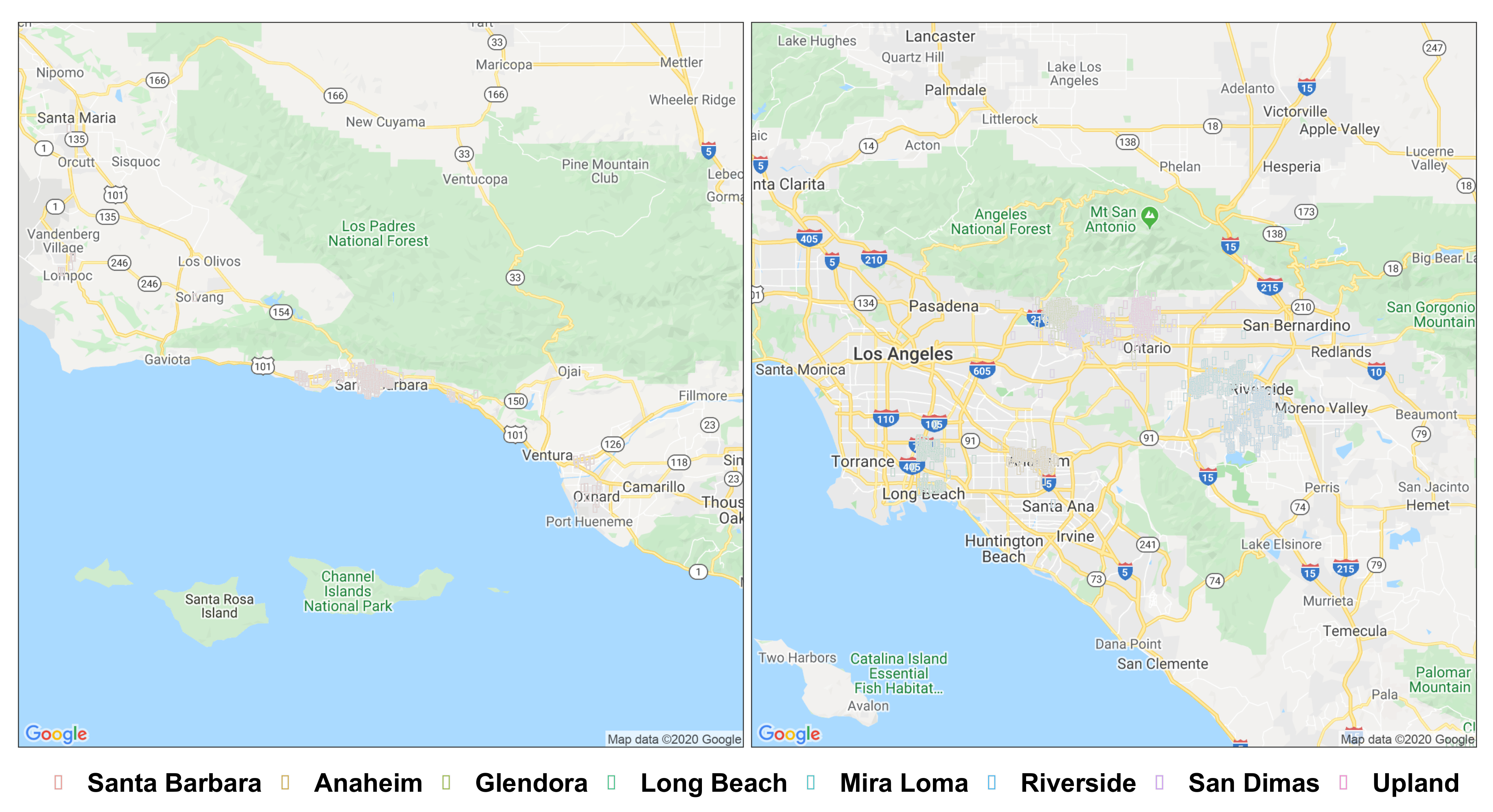
Since its inception in the early 1990s, the Southern California Children’s Health Study (CHS) has enrolled over 11,000 children in a series of five cohorts. In this study, we focused on the most recent cohort that began in 2003, enrolling approximately 3,000 children at age 6–7 years, and followed until 2012 when they were 15–16 years old. These children resided and went to school in eight communities in the greater Los Angeles, California area: Anaheim, Glendora, Long Beach, Mira Loma, Riverside, Santa Barbara, San Dimas, and Upland (Figure 1).
From 2007–2012, pulmonary function tests were conducted on each child by trained respiratory staff, measuring FEV and FVC with pressure transducer-based spirometers (ScreenStar Spirometers, Morgan Scientific, Haverhill, Massachusetts, USA). A written questionnaire was also administered to obtain information including age, sex, self-identified race and ethnic background, parental education, occurrences of acute respiratory illness, exercise, tobacco-smoke exposure (personal smoking or environmental), and housing characteristics (air conditioning, age of house, presence of mildew, pets in the home). Ethnic background in the CHS specifically relates to Hispanic ancestry, identifying Caucasian subjects with Hispanic and non-Hispanic ethnicity [41]. Study protocols were approved by the Institutional Review Board at the University of Southern California (USC), and additional details of CHS community and subject selection have been previously reported [42,43].
2.5. Exposure Estimation Methods
We expand upon our previous work [22,35] to include MISR aerosol properties of absorption (absorbing or non-absorbing), shape (spherical or nonspherical), and type provided by 74 weighted aerosol optical depths (mixtures) [21] to predict PM and PM SO, NO, EC, and dust. We matched daily PM and PM speciation measurements from ground monitors to the nearest available MISR pixel within 4.4 km (Figure A2) and then further matched them to the nearest gridMET pixel within 4 km. As some PM monitors are close to each other, it is possible they share the same MISR or gridMET pixel. In these instances, we used an algorithm to pair the shared MISR/gridMET pixel to the nearest monitor, and the remaining monitors were paired with the next available MISR/gridMET pixel within 4.4/4 km. If there were no other available MISR/gridMET pixels within an appropriate distance, the PM measurement on that day for that monitor was removed in order to avoid duplicating AOD and meteorological data in the dataset.
We trained the PM models on 70% of the data using 5-fold CV and assessed performance of the best model on the remaining 30%. We also trained the PM speciation models on 70% of the data with 5-fold CV and tested on 30%, but repeated the process 20 times to assess model stability due to much smaller sample sizes. Five machine learning methods were considered: Ridge regression, Least Absolute Shrinkage and Selection Operator (LASSO), Gradient Boosting (GBM), Random Forests (RF), and Support Vector Machines (SVM), all within a regression setting. Inputs to the models were meteorology and either the MISR AOD products or the 74 MISR AOD mixtures. The optimal model for each pollutant was chosen based on its test as the primary metric and its test RMSE as the secondary metric. We further supplemented the model with geospatial (coordinates of MISR pixels projected to UTM zone 11) and temporal (Julian date and month) predictors. The best predicting model for each pollutant was trained on the full dataset prior to estimating exposures for the epidemiological assessment.
2.6. Epidemiological Methods
To examine the association between air pollution exposure and lung function during the children’s critical period of development, we focused on pulmonary function tests (FEV and FVC) taken at ages 15–16 (2011–2012). During each assessment visit, the study participants reported their current addresses, which were geocoded. We identified MISR aerosol optical depth and gridMET meteorological data within 4.4 km of each study participant’s residence for the 12 months prior to their pulmonary function test, and predicted PM, NO, SO, EC, and dust concentrations spatially and temporally specific to each child. The 12-month means of these air pollutant estimates were assigned as exposures of interest for each child.
We fitted single-pollutant models to examine the effects of each predicted air pollutant exposure on lung function. Multi-pollutant models were also fitted to assess whether multiple predicted exposures better informed the associations of interest. Using mixed-effects models, we adjusted for study community with a random intercept and for biological characteristics such as age, gender, height, BMI, and race/ethnicity as fixed effects. Based on previous studies of the CHS, log transformation of FEV and FVC as well as quadratic terms for height and BMI were considered [1,3,4,6]. We separately fitted similar models with central-site PM to compare with MISR-derived PM models. Akaike information criterion (AIC) was used as the main metric for model comparison and Bayesian information criterion (BIC), which favors more parsimonious models, as the secondary metric. Generalized variance inflation factor was calculated to assess potential collinearity among the predictors (using GVIF as the cutoff).
3. Results
3.1. Exposure Estimation
From March 2000 through December 2018, there were 2828 days where MISR had complete retrievals of AOD products that could be matched to EPA-PM stations, resulting in a dataset of . In the same period, there were 2864 days where MISR had complete retrievals of AOD mixtures that could be matched to EPA-PM stations, resulting in a dataset of . While there were more days with successful AOD mixtures retrieved, the AOD-products datasets was larger because AOD-products were successfully retrieved in more locations per day compared to AOD mixtures. In a similar time frame (ending in July 2018), MISR had 698 days with AOD-products data and 544 days with AOD-mixtures data that were matched to PM speciation concentrations from CSN sites in California, resulting in datasets of sizes for models using AOD products and for models using AOD mixtures.
Non-linear machine learning methods (GBM, RF, and SVM) generally predicted better than linear methods (ridge and LASSO) for all exposures of interest and for both AOD-products and AOD-mixtures models. Although the AOD-mixtures models for PM had a smaller training dataset, the increase in model complexity with 74 AOD mixtures versus 6 AOD products led to much more time-expensive model fitting. We experimented with a smaller sample size () but the AOD-mixtures models did not perform better than the AOD-products models. The GBM model using AOD products had the best performance for PM () (Table 1).
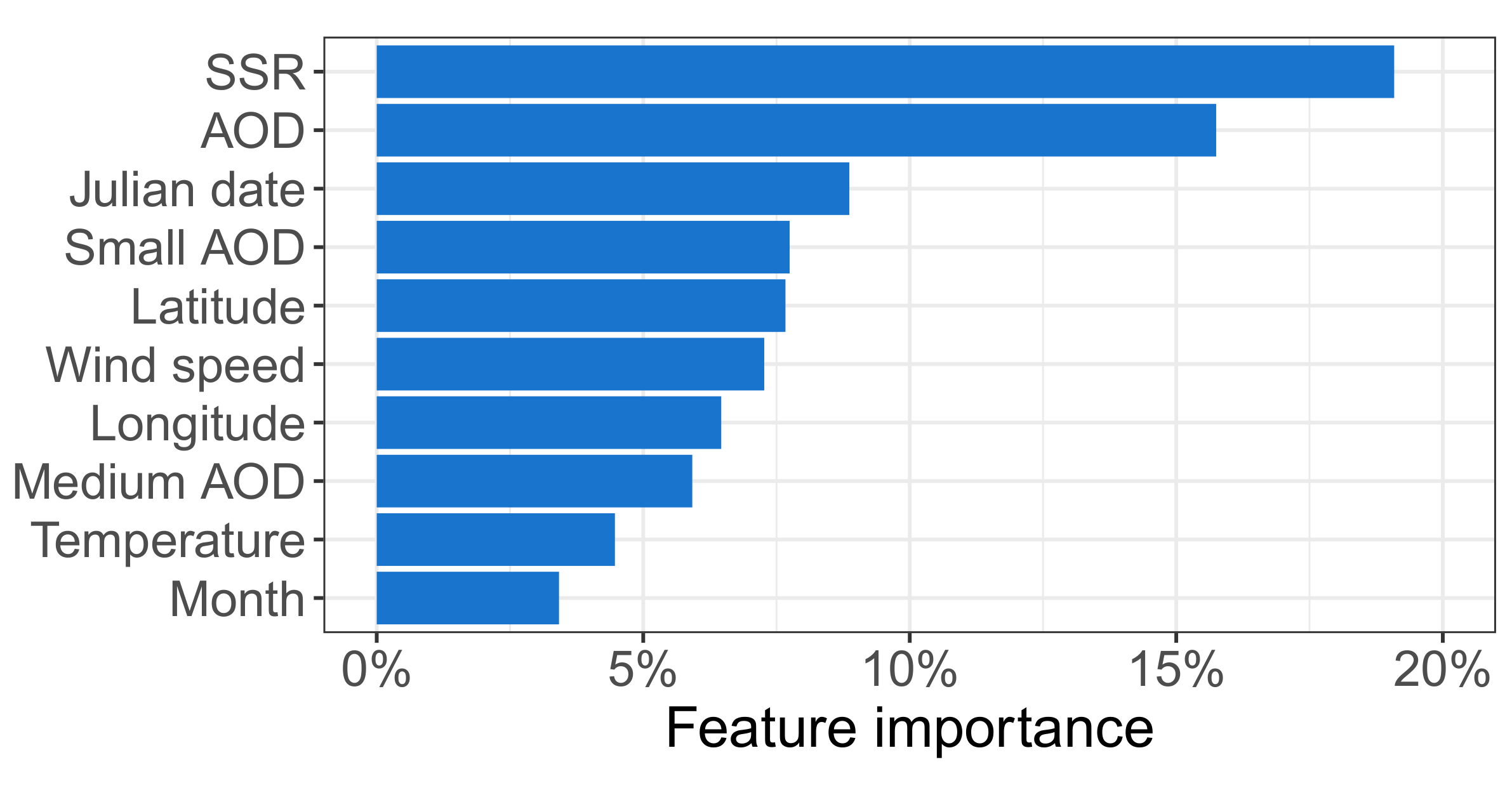
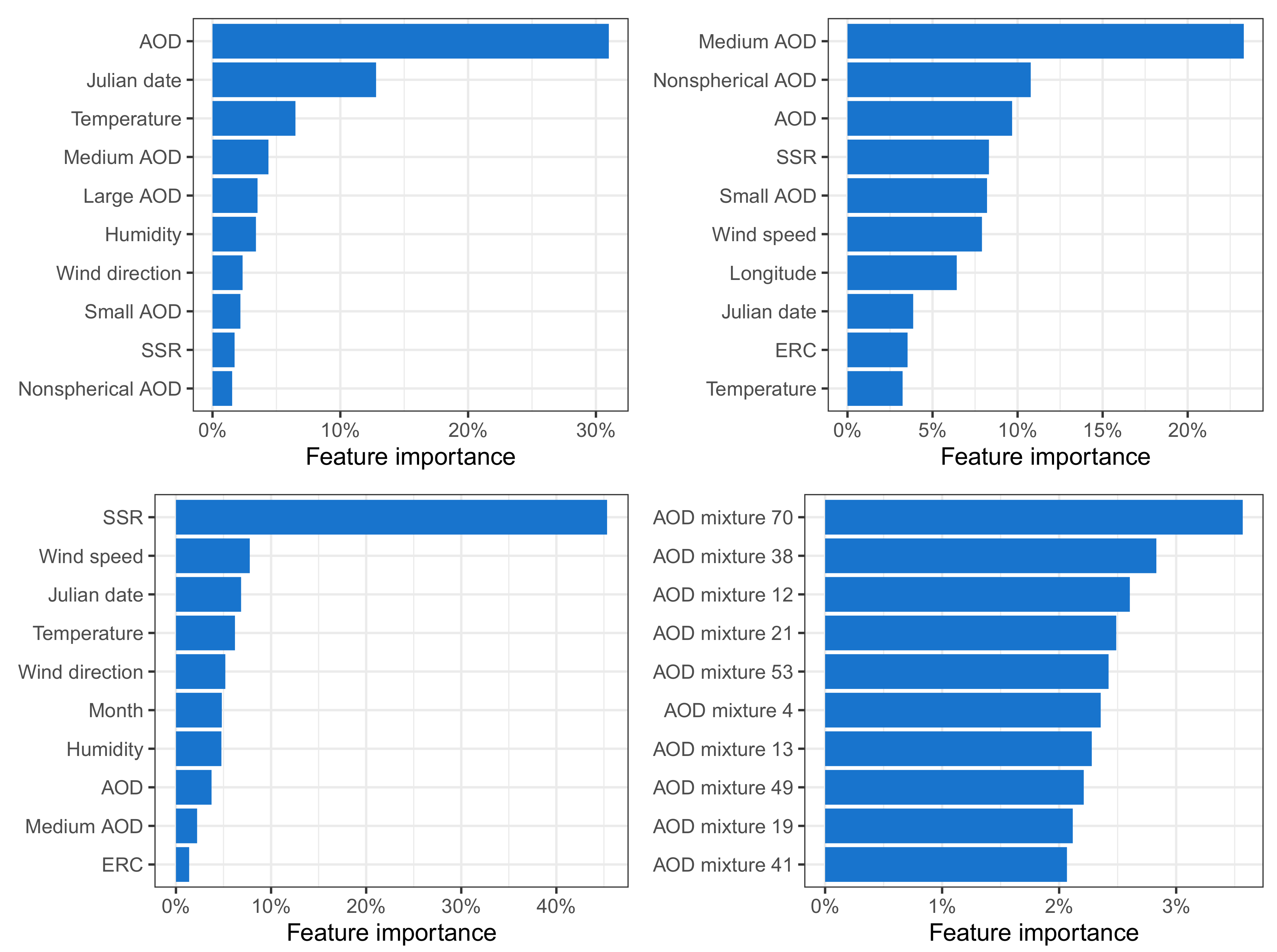
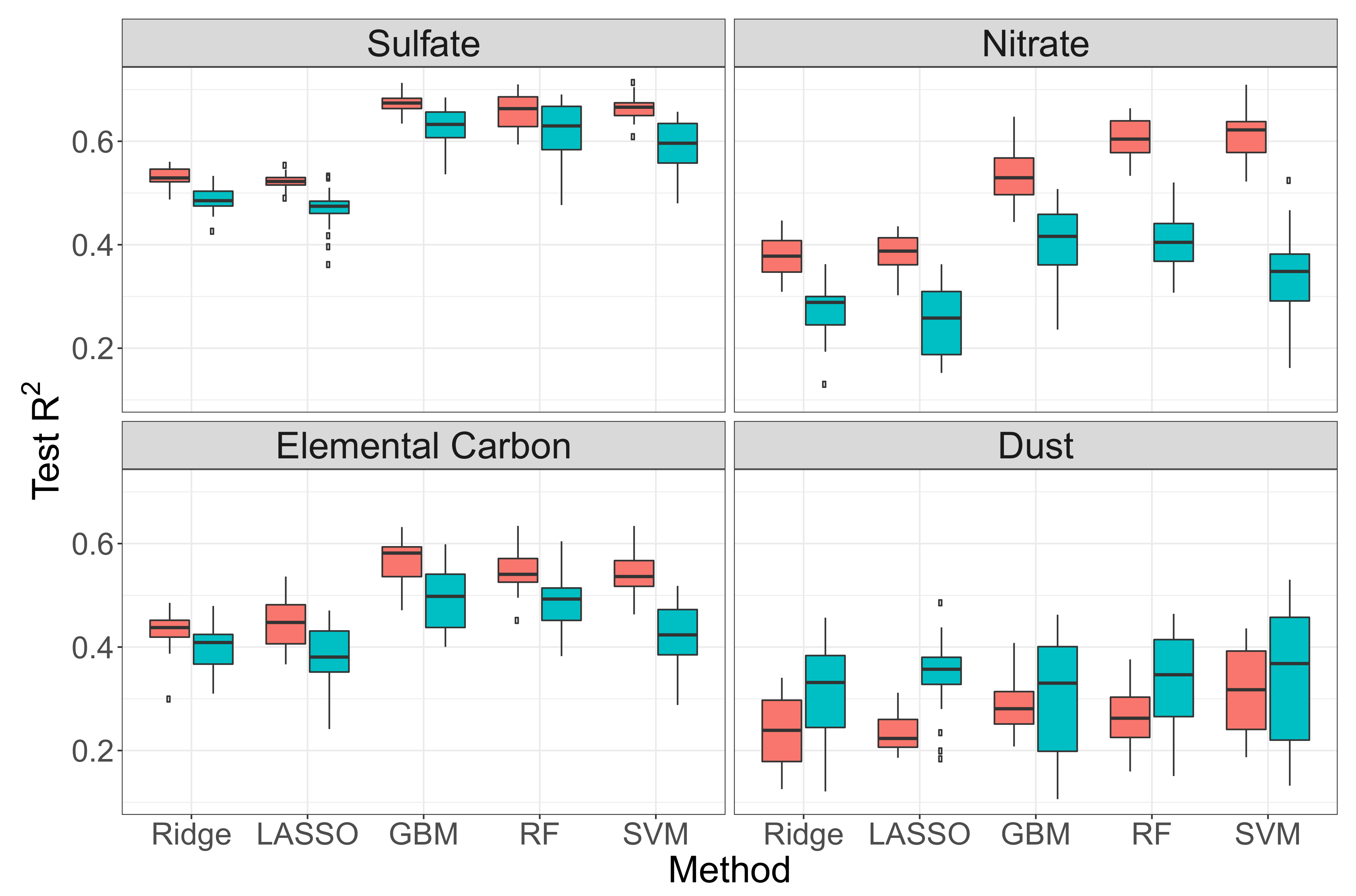
The boxplots of test (Figure A3) for PM speciation models show that AOD-products models outperformed AOD-mixtures models and did so consistently (narrower boxplots) with the exception of dust, where AOD-mixtures models performed better. The best test for SO and NO was 0.71, EC 0.63, and dust 0.53 (Table 1). The most important variables for PM include an interpretable mix of AOD, small and medium AOD, as well as meteorological variables (surface shortwave radiation, wind speed, and temperature) (Figure 2). Similar variables were important for SO and NO, but nonspherical AOD played a larger role in both (Figure 3). Interestingly, AODs only ranked 8th and 9th for EC, with meteorology and temporal indicators playing a larger role in its prediction. Finally, most important for dust were AOD mixtures relating primarily to dust (mixtures 70 and 53) and non-absorbing (mixtures 4, 12, 13, 19, 21) particles.
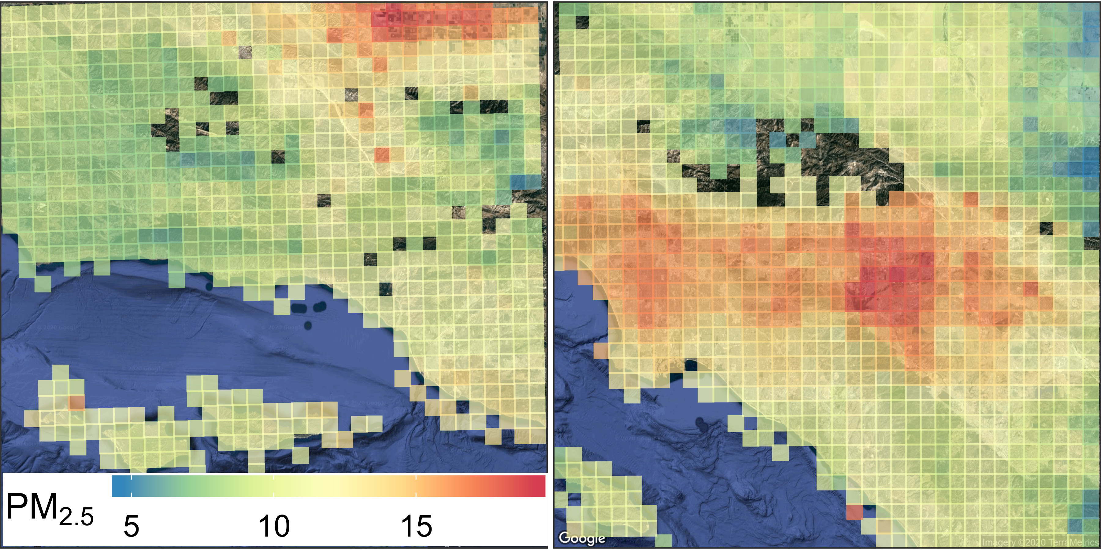
MISR AOD-products were used to predict all exposures except for dust, which was predicted using MISR AOD mixtures. Figure 4 and Figure 5 show 6-year (2007–2012) means of the predicted air pollution exposures over greater Los Angeles and Santa Barbara. Over this period the correlation between annual mean MISR-derived PM and PM speciation with its central-site counterpart were positive and statistically significant, with Spearman and (Table A1).
3.2. Health Outcomes
There were 1206 children assessed in 2011–2012 with mean age 15.2 (SD ) years, whose geocoded addresses were linked with MISR-derived exposure estimates. Summary statistics of the study population, including gender, height, weight, race/ethnicity, and study community, are shown in Table 2. Both FEV and FVC were significantly higher among boys compared to girls; mean FEV was 4111 mL among boys and 3304 mL among girls (t-test ), mean FVC was 4801 mL among boys and 3752 mL among girls (t-test ). Among race/ethnicity groups, there were significant differences in mean FEV and FVC with one-way ANOVA test and , respectively (Table A2). The associations between biological factors and lung function remained significant when evaluated in fully adjusted models (Table A3).
In single-pollutant mixed models adjusted for biological characteristics, MISR-derived PM, SO, and dust were significantly associated with decreases in FEV, and SO and NO were significantly associated with decreases in FVC. Notably, central-site PM was not associated with either lung function measure (Table 3). Among multi-pollutant models, we did not find any grouping of two or more pollutants to be significantly associated with FEV or FVC. Furthermore, while certain multi-pollutant models achieved modest reductions in AIC, none outperformed single-pollutant models in BIC. Log transformation of the lung function measures, with slight improvements in normality on Q-Q plots, did not improve model fit for either outcomes. Collinearity was not an issue in any of the models (all GVIF ).
Effect estimates in Table 3 represent the difference in mean FEV and FVC between the highest and the lowest exposure level for each pollutant in single-pollutant models. After accounting for biological and community effects in single-pollutant mixed models, FEV on average decreased by 131 mL (95% CI: ) per 10.7-µg/m increase in PM, by 158 mL (95% CI: ) per 1.2-µg/m in SO, and by 177 mL (95% CI: ) per 1.6-µg/m increase in dust. Meanwhile, FVC on average decreased by 175 mL (95% CI: ) per 1.2-µg/m increase in SO and by 212 mL (95% CI: ) per 2.5-µg/m increase in NO.
4. Discussion
In this study, we used satellite observations of AOD, characterized by size, shape, and absorption properties as well as fractionated into 74 mixtures, to estimate PM and select PM chemical components. We then incorporated these estimates into an epidemiological assessment of their association with children’s lung function. In terms of exposure estimation, MISR AOD products resulted in better and more robust estimates than did AOD mixtures, except for dust. Non-linear models (GBM, RF, and SVM) performed better than linear models (Ridge and LASSO), which was consistent with previous studies where linear models were inadequate in explaining the relationship between AOD and ground-monitored PM [22,35,46]. Although MISR aerosol data have coarser temporal and spatial resolution compared to MAIAC (every 3–5 days vs. daily and 4.4 km vs. 1 km, respectively), our model achieved high prediction performance (Table 1) using MISR-specific data products on size, shape, and absorption, which proved vital in the prediction models. At least two MISR AOD products were among the five most important features for predicting PM, SO, and NO, and the ten most important features for predicting dust were all AOD mixtures (Figure 2 and Figure 3).
Our PM prediction performance was similar to those by Sorek-Hamer et al. [46], who modeled PM using AOD data from MODIS (Collection 5 Level 2) and the Ozone Monitoring Instrument (OMI) at 10-km resolution over the Central Valley in California. In Southern California, we improved upon previous work that predicted PM, SO, and NO by Franklin et al. [22], whose meteorological data from NOAA weather stations did not provide the spatial coverage of gridMET data. Surface shortwave radiation provided by gridMET was also among the most important predictors for PM, NO, and EC (Figure 2 and Figure 3). Our PM, SO, NO, and EC models performed comparably to those by Meng et al. [23], who reconstructed fractional AOD using the AOD mixtures (V22) while we relied on MISR AOD products (V23).
One limitation in our PM speciation prediction models is the scarcity of data. As the number of CSN sites in California increased from 3 in 2000 to 19 in 2013 and decreased to 16 in 2018 (California PM mass sites increased from 95 in 2000 to 157 in 2018), spatial coverage was certainly restricted (Figure A1). Furthermore, the locations of these sparsely available monitors are not necessarily representative of the population density of Southern California. We used the coordinates of MISR pixels, which lacked a fixed grid, instead of monitoring sites as geospatial predictors to help mitigate this problem by introducing additional spatial variability. We also attempted prediction models for PM and SO (detailed results not reported here) to compare with our previous work over Mongolia [35]. While PM models performed about the same, i.e., average test , SO models over California performed much worse, with average test (vs. test over Ulaanbaatar). Poor prediction performance for SO was likely due to much lower concentrations of SO in California (mean SO ppb in 2000–2018) compared to Ulaanbaatar (9.7 ppb in 2008–2017), where SO is the more dominant source of PM. For the epidemiological purposes of the current study, we focused on models predicting PM and its chemical components.
This study is unique in estimating air pollution exposure specifically to the residence and follow-up period of each subject. Previously, exposures were assigned using annual means from one central air pollution monitoring site for each study community [5,6,42], even if the children might have lived far away from these sites. Furthermore, the follow-up period spanned about 211 days, yet the annual means of central-site air pollutants for each community were calculated using a fixed time window. Leveraging MISR aerosol and gridMET meteorological data, we improved upon these limitations by assigning exposures that were spatially within 4.4 km of where each child lived and temporally specific to the 12 months prior to each child’s assessment visit. Nevertheless, our exposure prediction models are not without unexplained residual variance; our best models had CV R from 0.53 (dust) to 0.71 (SO, NO). As noted by Alexeeff et al. [10], there can be 1–5% upward bias in subsequent health effects estimates when exposure predictions have performance statistics in the range we observed, and their standard errors may be underestimated. It is difficult to mitigate these issues due to imperfect exposure models, but it is worth keeping in mind while interpreting our epidemiological results.
While this is not the first study using AOD-derived PM concentration in an epidemiological context, it is the first examining satellite-derived PM speciation. Previous studies of AOD-derived PM include Rice et al. [27], who found that each 2 µg/m increase in AOD-derived PM was associated with a 28 mL ( to 0.2 mL) decrease in forced vital capacity (FVC) and higher odds of forced expiratory volume in 1 second (FEV) being less than 80% predicted (OR , 1.03 to 1.93). In another study, AOD-derived PM concentrations were associated with an increased rate of asthma onset (HR , 1.28 to 1.33) in Quebec [28].
Similar to previous evaluations of the CHS [3,5,6], biological characteristics (age, gender, race/ethnicity, height, height squared, BMI, and BMI squared) were significantly associated with both measurements of lung function (Table A3). With these adjustments, several MISR-derived estimates of air pollutants were able to explain the residual differences in lung function measurements among the children. Another strength of this study is identifying the effect of specific PM chemical components on lung function. While MISR-derived PM was significantly associated with decreases in FEV, its effect, measured as the difference in FEV between the highest and lowest exposure level for each pollutant, is smaller than those of SO and dust (Table 3). Similarly, although FVC was only marginally statistically significantly associated with MISR-derived PM, its associations with SO and NO were clinically significant. In California, secondary aerosols including nitrate and sulfate have been shown to be the most abundant contributors to ambient PM, with nitrate accounting for as much as 55% of the total mass [47]. Geologic dust can also contribute up to 20% of the mass in summer in more arid regions of Southern California. Importantly, we were able to distinguish that these PM species had differentially stronger associations with children’s FEV and FVC.
Urman et al. [3], who examined the cross-sectional effect of central-site air pollution on lung function in the same cohort but at an earlier visit when the children were at ages 11–12, found central-site PM to be significant with both log-transformed FEV and FVC. In our study, we did not find central-site PM to be significant with either outcomes. We did find MISR-derived PM to be significantly associated with log-transformed FEV, with a similar effect size, but not with log-transformed FVC. Children exposed to the highest level of MISR-derived PM on average were (95% CI: ) lower in FEV compared to those exposed to the lowest level. In the same CHS cohort and during the same follow-up period, Franklin and Fruin [4] found a significant association between NO on FVC when adjusted for traffic-related noise exposure. We found a similarly significant relationship between NO and FVC where an IQR increase in NO (0.64 µg/m) is associated with 53 mL decrease in FVC (95% CI: ).
5. Conclusions
We have shown in this study that MISR AOD observations distinguishing size, shape, absorption and mixture properties can aid in predicting PM and its chemical speciation including SO, NO, EC, and dust, particularly when supplemented with spatio-temporal information and high-resolution meteorological data. Machine learning methods such as Gradient Boosting and Support Vector Machines were more suitable for characterizing the non-linear relationships between air pollutants and AOD. We further showed that different MISR-derived PM composition, estimated specifically to the residence and follow-up period of CHS study participants, were able to explain clinically significant differences in lung function measurements FEV and FVC. This demonstrates that satellite-observed aerosol data products can be incorporated to strengthen epidemiological studies investigating the health effects of environmental pollution. Epidemiological assessments will only be made more viable, particularly as the quality of remote sensing data and estimation models continue to improve and exposure measurement error decreases.
Author Contributions
Conceptualization, M.F.; methodology, K.C, M.F., W.J.G.; formal analysis, K.C.; data curation, K.C., M.F.; writing—original draft preparation, K.C., M.F.; writing—review and editing, K.C., M.F., W.J.G.; supervision, M.F.; project administration, M.F.; funding acquisition, M.F. All authors have read and agreed to the published version of the manuscript.
Funding
This research was funded by National Aeronautics and Space Administration grant number NNN12AA01C and under contract to the Health Effects Institute (HEI), an organization jointly funded by the United States Environmental Protection Agency (EPA) (Assistance Award No. CR-83590201) and certain motor vehicle and engine manufacturers.
Acknowledgments
The authors would like to thank Olga Kalashnikova, Michael Garay, and Dave Diner from the Jet Propulsion Laboratory’s MISR team for their guidance and support.
Conflicts of Interest
The authors declare no conflict of interest.
Abbreviations
The following abbreviations are used in this manuscript:
| ANOVA | Analysis of variance |
| AOD | Aerosol Optical Depth |
| CHS | Children’s Health Study |
| CSN | Chemical Speciation Network |
| FEV | Forced expiratory volume in 1 second |
| FVC | Forced vital capacity |
| MAIAC | MultiAngle Implementation of Atmospheric Correction |
| MISR | Multiangle Imaging SpectroRadiometer |
| MODIS | MoDerate resolution Imaging Spectroradiometer |
| NO | Nitrate |
| NO | Nitrogen Dioxide |
| NO | Nitrogen Oxides |
| PM | Particulate Matter |
| PM | Particulate Matter with aerodynamic diameter ≤ 2.5 m |
| PM | Particulate Matter with aerodynamic diameter ≤ 10 m |
| PM | Particulate Matter |
| SO | Sulfate |
Appendix A

Table A1.
Spearman correlation coefficients for annual means of air pollution exposures during the three CHS follow-up periods (2007–2012).
Table A1.
Spearman correlation coefficients for annual means of air pollution exposures during the three CHS follow-up periods (2007–2012).
| PM | PM | SO | NO | EC | Dust | |
|---|---|---|---|---|---|---|
| PM | 1 | 0.68 | 0.55 | 0.34 | 0.29 | 0.68 |
| PM | 1 | 0.74 | 0.59 | 0.15 | 0.38 | |
| SO | 1 | 0.92 | 0.29 | 0.14 | ||
| NO | 1 | 0.37 | ||||
| EC | 1 | 0.32 | ||||
| Dust | 1 |
Central-site PM; MISR-derived PM
Table A2.
Mean (SD) of FEV and FVC by gender and race/ethnicity.
| FEV | FVC | |
|---|---|---|
| Gender | ||
| Female | 3304 (453) | 3752 (537) |
| Male | 4111 (680) | 4801 (797) |
| Race/Ethnicity | ||
| White | 3746 (665) | 4377 (831) |
| Asian | 3492 (635) | 3892 (746) |
| Black | 3271 (548) | 3777 (683) |
| Hispanic | 3715 (733) | 4258 (884) |
| Others | 3634 (688) | 4162 (774) |
Table A3.
Effect estimates of biological characteristics on lung function in mixed models without air pollution exposure.
Table A3.
Effect estimates of biological characteristics on lung function in mixed models without air pollution exposure.
| FEV | FVC | |||
|---|---|---|---|---|
| Characteristic | Estimate | 95% CI | Estimate | 95% CI |
| Age (year) | 121 | 112 | ||
| Gender | ||||
| Girls | (ref.) | – | (ref.) | – |
| Boys | 317 | 440 | ||
| Race/ethnicity | ||||
| White | (ref.) | – | (ref.) | – |
| Asian | () | ) | ||
| Black | () | () | ||
| Hispanic | 96 | () | 40 | () |
| Others | 52 | () | () | |
| Height (cm) | 47 | () | 59 | () |
| Height | 0.3 | () | 0.5 | () |
| BMI (kg/m) | 35.7 | () | 49 | () |
| BMI | () | () | ||
Figure A1.
Maps of EPA PM2.5 monitoring sites (left) and CSN monitoring sites (right) from 2000 to 2018.
Figure A1.
Maps of EPA PM2.5 monitoring sites (left) and CSN monitoring sites (right) from 2000 to 2018.

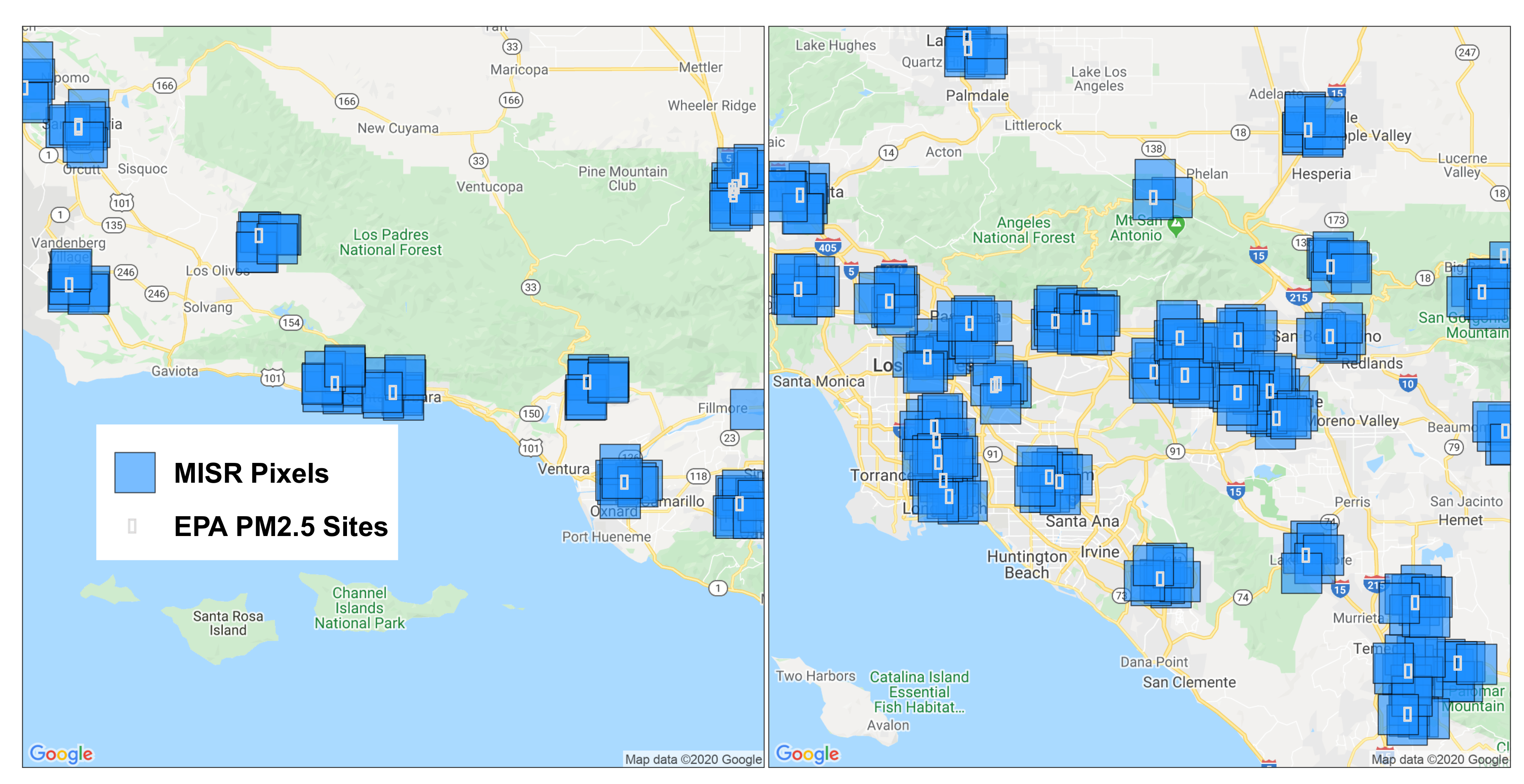
Figure A2.
Maps of EPA PM2.5 monitoring sites and the MISR pixels within 4.4 km of each site, in Santa Barbara (left) and other communities (right).
Figure A2.
Maps of EPA PM2.5 monitoring sites and the MISR pixels within 4.4 km of each site, in Santa Barbara (left) and other communities (right).

Figure A3.
Boxplots of test R from 20 iterations of each machine learning method applied to predicting PM speciation, in AOD-products (coral) and AOD-mixtures (teal) models.
Figure A3.
Boxplots of test R from 20 iterations of each machine learning method applied to predicting PM speciation, in AOD-products (coral) and AOD-mixtures (teal) models.

References
- Gauderman, W.J.; Vora, H.; McConnell, R.; Berhane, K.; Gilliland, F.; Thomas, D.; Lurmann, F.; Avol, E.; Kunzli, N.; Jerrett, M.; et al. Effect of exposure to traffic on lung development from 10 to 18 years of age: A cohort study. Lancet 2007, 369, 571–577. [Google Scholar] [CrossRef]
- McConnell, R.; Islam, T.; Shankardass, K.; Jerrett, M.; Lurmann, F.; Gilliland, F.; Gauderman, J.; Avol, E.; Künzli, N.; Yao, L.; et al. Childhood incident asthma and traffic-related air pollution at home and school. Environ. Health Perspect. 2010, 118, 1021–1026. [Google Scholar] [CrossRef] [PubMed] [Green Version]
- Urman, R.; McConnell, R.; Islam, T.; Avol, E.L.; Lurmann, F.W.; Vora, H.; Linn, W.S.; Rappaport, E.B.; Gilliland, F.D.; Gauderman, W.J. Associations of children’s lung function with ambient air pollution: Joint effects of regional and near-roadway pollutants. Thorax 2014, 69, 540–547. [Google Scholar] [CrossRef] [Green Version]
- Franklin, M.; Fruin, S. The role of traffic noise on the association between air pollution and children’s lung function. Environ. Res. 2017, 157, 153–159. [Google Scholar] [CrossRef] [PubMed]
- Gauderman, W.J.; Avol, E.; Gilliland, F.; Vora, H.; Thomas, D.; Berhane, K.; McConnell, R.; Kuenzli, N.; Lurmann, F.; Rappaport, E.; et al. The Effect of Air Pollution on Lung Development from 10 to 18 Years of Age. N. Engl. J. Med. 2004, 351, 1057–1067. [Google Scholar] [CrossRef] [Green Version]
- Gauderman, W.J.; Urman, R.; Avol, E.; Berhane, K.; McConnell, R.; Rappaport, E.; Chang, R.; Lurmann, F.; Gilliland, F. Association of Improved Air Quality with Lung Development in Children. N. Engl. J. Med. 2015, 372, 905–913. [Google Scholar] [CrossRef] [Green Version]
- AQS (Air Quality System) User Guide. Available online: https://www.epa.gov/aqs/aqs-user-guide (accessed on 16 January 2020).
- Ryan, P.H.; Lemasters, G.K. A review of land-use regression models for characterizing intraurban air pollution exposure. Inhal. Toxicol. 2007, 19, 127–133. [Google Scholar] [CrossRef] [Green Version]
- Franklin, M.; Vora, H.; Avol, E.; McConnell, R.; Lurmann, F.; Liu, F.; Penfold, B.; Berhane, K.; Gilliland, F.; Gauderman, W.J. Predictors of intra-community variation in air quality. J. Expo. Sci. Environ. Epidemiol. 2012, 22, 135–147. [Google Scholar] [CrossRef] [Green Version]
- Alexeeff, S.E.; Schwartz, J.; Kloog, I.; Chudnovsky, A.; Koutrakis, P.; Coull, B.A. Consequences of kriging and land use regression for PM2.5 predictions in epidemiologic analyses: Insights into spatial variability using high-resolution satellite data. J. Expo. Sci. Environ. Epidemiol. 2015, 25, 138–144. [Google Scholar] [CrossRef] [Green Version]
- Brauer, M.; Amann, M.; Burnett, R.T.; Cohen, A.; Dentener, F.; Ezzati, M.; Henderson, S.B.; Krzyzanowski, M.; Martin, R.V.; Van Dingenen, R.; et al. Exposure assessment for estimation of the global burden of disease attributable to outdoor air pollution. Environ. Sci. Technol. 2012, 46, 652–660. [Google Scholar] [CrossRef] [Green Version]
- De Sherbinin, A.; Levy, M.A.; Zell, E.; Weber, S.; Jaiteh, M. Using satellite data to develop environmental indicators. Environ. Res. Lett. 2014, 9, 084013. [Google Scholar] [CrossRef]
- Van Donkelaar, A.; Martin, R.V.; Spurr, R.J.; Drury, E.; Remer, L.A.; Levy, R.C.; Wang, J. Optimal estimation for global ground-level fine particulate matter concentrations. J. Geophys. Res. Atmos. 2013, 118, 5621–5636. [Google Scholar] [CrossRef] [Green Version]
- Van Donkelaar, A.; Martin, R.V.; Brauer, M.; Boys, B.L. Use of satellite observations for long-term exposure assessment of global concentrations of fine particulate matter. Environ. Health Perspect. 2015, 123, 135–143. [Google Scholar] [CrossRef] [PubMed] [Green Version]
- Shaddick, G.; Thomas, M.L.; Green, A.; Brauer, M.; van Donkelaar, A.; Burnett, R.; Chang, H.H.; Cohen, A.; Dingenen, R.V.; Dora, C.; et al. Data integration model for air quality: A hierarchical approach to the global estimation of exposures to ambient air pollution. J. R. Stat. Soc. Ser. Appl. Stat. 2018, 67, 231–253. [Google Scholar] [CrossRef]
- Lyapustin, A.; Wang, Y.; Korkin, S.; Huang, D. MODIS Collection 6 MAIAC algorithm. Atmos. Meas. Tech. 2018, 11, 5741–5765. [Google Scholar] [CrossRef] [Green Version]
- Diner, D.J.; Beckert, J.C.; Bothwell, G.W.; Rodriguez, J.I. Performance of the MISR instrument during its first 20 months in earth orbit. IEEE Trans. Geosci. Remote Sens. 2002, 40, 1449–1466. [Google Scholar] [CrossRef]
- Garay, M.J.; Kalashnikova, O.V.; Bull, M.A. Development and assessment of a higher-spatial-resolution (4.4 km) MISR aerosol optical depth product using AERONET-DRAGON data. Atmos. Chem. Phys. 2017, 17, 5095–5106. [Google Scholar] [CrossRef] [Green Version]
- Van Donkelaar, A.; Martin, R.V.; Brauer, M.; Kahn, R.; Levy, R.; Verduzco, C.; Villeneuve, P.J. Global estimates of ambient fine particulate matter concentrations from satellite-based aerosol optical depth: Development and application. Environ. Health Perspect. 2010, 118, 847–855. [Google Scholar] [CrossRef] [Green Version]
- Van Donkelaar, A.; Martin, R.V.; Li, C.; Burnett, R.T. Regional Estimates of Chemical Composition of Fine Particulate Matter Using a Combined Geoscience-Statistical Method with Information from Satellites, Models, and Monitors. Environ. Sci. Technol. 2019, 53, 2595–2611. [Google Scholar] [CrossRef] [Green Version]
- Kahn, R.A.; Gaitley, B.J. An analysis of global aerosol type as retrieved by MISR. J. Geophys. Res. Atmos. 2015, 120, 4248–4281. [Google Scholar] [CrossRef]
- Franklin, M.; Kalashnikova, O.V.; Garay, M.J. Size-resolved particulate matter concentrations derived from 4.4 km-resolution size-fractionated Multi-angle Imaging SpectroRadiometer (MISR) aerosol optical depth over Southern California. Remote. Sens. Environ. 2017, 196, 312–323. [Google Scholar] [CrossRef]
- Meng, X.; Garay, M.J.; Diner, D.J.; Kalashnikova, O.V.; Xu, J.; Liu, Y. Estimating PM2.5 speciation concentrations using prototype 4.4 km-resolution MISR aerosol properties over Southern California. Atmos. Environ. 2018, 181, 70–81. [Google Scholar] [CrossRef]
- Burnett, R.T.; Pope, C.A.; Ezzati, M.; Olives, C.; Lim, S.S.; Mehta, S.; Shin, H.H.; Singh, G.; Hubbell, B.; Brauer, M.; et al. An integrated risk function for estimating the global burden of disease attributable to ambient fine particulate matter exposure. Environ. Health Perspect. 2014, 122, 397–403. [Google Scholar] [CrossRef] [PubMed]
- Cohen, A.J.; Brauer, M.; Burnett, R.; Anderson, H.R.; Frostad, J.; Estep, K.; Balakrishnan, K.; Brunekreef, B.; Dandona, L.; Dandona, R.; et al. Estimates and 25-year trends of the global burden of disease attributable to ambient air pollution: An analysis of data from the Global Burden of Diseases Study 2015. Lancet 2017, 389, 1907–1918. [Google Scholar] [CrossRef] [Green Version]
- Kloog, I.; Nordio, F.; Coull, B.A.; Schwartz, J. Incorporating local land use regression and satellite aerosol optical depth in a hybrid model of spatiotemporal PM2.5 exposures in the mid-atlantic states. Environ. Sci. Technol. 2012, 46, 11913–11921. [Google Scholar] [CrossRef] [PubMed] [Green Version]
- Rice, M.B.; Rifas-Shiman, S.L.; Litonjua, A.A.; Oken, E.; Gillman, M.W.; Kloog, I.; Luttmann-Gibson, H.; Zanobetti, A.; Coull, B.A.; Schwartz, J.; et al. Lifetime exposure to ambient pollution and lung function in children. Am. J. Respir. Crit. Care Med. 2016, 193, 881–888. [Google Scholar] [CrossRef] [Green Version]
- Tétreault, L.F.; Doucet, M.; Gamache, P.; Fournier, M.; Brand, A.; Kosatsky, T.; Smargiassi, A. Childhood exposure to ambient air pollutants and the onset of asthma: An administrative cohort study in Québec. Environ. Health Perspect. 2016, 124, 1276–1282. [Google Scholar] [CrossRef] [Green Version]
- Air Data: Air Quality Data Collected at Outdoor Monitors Across the US. Available online: https://www.epa.gov/outdoor-air-quality-data (accessed on 14 January 2020).
- Chemical Speciation Network (CSN). Available online: https://www.epa.gov/amtic/chemical-speciation-network-csn (accessed on 14 January 2020).
- Chow, J.C.; Lowenthal, D.H.; Chen, L.W.; Wang, X.; Watson, J.G. Mass reconstruction methods for PM2.5: A review. Air Qual. Atmos. Health 2015, 8, 243–263. [Google Scholar] [CrossRef] [Green Version]
- Chow, J.C.; Watson, J.G.; Ashbaugh, L.L.; Magliano, K.L. Similarities and differences in PM10 chemical source profiles for geological dust from the San Joaquin Valley, California. Atmos. Environ. 2003, 37, 1317–1340. [Google Scholar] [CrossRef]
- Witek, M.L.; Garay, M.J.; Diner, D.J.; Bull, M.A.; Seidel, F.C. New approach to the retrieval of AOD and its uncertainty from MISR observations over dark water. Atmos. Meas. Tech. 2018, 11, 429–439. [Google Scholar] [CrossRef] [Green Version]
- Kahn, R.A.; Gaitley, B.J.; Garay, M.J.; Diner, D.J.; Eck, T.F.; Smirnov, A.; Holben, B.N. Multiangle Imaging SpectroRadiometer global aerosol product assessment by comparison with the Aerosol Robotic Network. J. Geophys. Res. Atmos. 2010, 115, D23209. [Google Scholar] [CrossRef]
- Franklin, M.; Chau, K.; Kalashnikova, O.V.; Garay, M.J.; Enebish, T.; Sorek-Hamer, M. Using multi-angle imaging spectro radiometer aerosol mixture properties for air quality assessment in Mongolia. Remote. Sens. 2018, 10, 1317. [Google Scholar] [CrossRef] [Green Version]
- Al-Saadi, J.; Szykman, J.; Pierce, R.B.; Kittaka, C.; Neil, D.; Chu, D.A.; Remer, L.; Gumley, L.; Prins, E.; Weinstock, L.; et al. Improving national air quality forecasts with satellite aerosol observations. Bull. Am. Meteorol. Soc. 2005, 86, 1249–1261. [Google Scholar] [CrossRef]
- gridMET - Climatology Lab. Available online: http://www.climatologylab.org/gridmet.html (accessed on 14 January 2020).
- Abatzoglou, J.T. Development of gridded surface meteorological data for ecological applications and modelling. Int. J. Climatol. 2013, 33, 121–131. [Google Scholar] [CrossRef]
- Smith, D.M.; Booth, B.B.B.; Dunstone, N.J.; Eade, R.; Hermanson, L.; Jones, G.S.; Scaife, A.A.; Sheen, K.L.; Thompson, V. Role of volcanic and anthropogenic aerosols in the recent global surface warming slowdown. Nat. Clim. Chang. 2016, 6, 936–940. [Google Scholar] [CrossRef]
- Freychet, N.; Tett, S.F.B.; Bollasina, M.; Wang, K.C.; Hegerl, G.C. The Local Aerosol Emission Effect on Surface Shortwave Radiation and Temperatures. J. Adv. Model. Earth Syst. 2019, 11, 806–817. [Google Scholar] [CrossRef]
- Weaver, G.M.; James Gauderman, W. Traffic-Related Pollutants: Exposure and Health Effects among Hispanic Children. Am. J. Epidemiol. 2018, 187, 45–52. [Google Scholar] [CrossRef]
- Peters, J.M.; Avol, E.; Navidi, W.; London, S.J.; Gauderman, W.J.; Lurmann, F.; Linn, W.S.; Margolis, H.; Rappaport, E.; Gong, H.; et al. A study of twelve Southern California communities with differing levels and types of air pollution: I. Prevalence of respiratory morbidity. Am. J. Respir. Crit. Care Med. 1999, 159, 760–767. [Google Scholar] [CrossRef]
- McConnell, R.; Berhane, K.; Yao, L.; Jerrett, M.; Lurmann, F.; Gilliland, F.; Künzli, N.; Gauderman, J.; Avol, E.; Thomas, D.; et al. Traffic, susceptibility, and childhood asthma. Environ. Health Perspect. 2006, 114, 766–772. [Google Scholar] [CrossRef] [Green Version]
- Friedman, J.H. Greedy Function Approximation: A Gradient Boosting Machine. Ann. Stat. 2001, 29, 1189–1232. [Google Scholar] [CrossRef]
- Cortez, P.; Embrechts, M.J. Using sensitivity analysis and visualization techniques to open black box data mining models. Inf. Sci. 2013, 225, 1–17. [Google Scholar] [CrossRef] [Green Version]
- Sorek-Hamer, M.; Strawa, A.W.; Chatfield, R.B.; Esswein, R.; Cohen, A.; Broday, D.M. Improved retrieval of PM2.5 from satellite data products using non-linear methods. Environ. Pollut. 2013, 182, 417–423. [Google Scholar] [CrossRef] [PubMed]
- Hasheminassab, S.; Daher, N.; Saffari, A.; Wang, D.; Ostro, B.D.; Sioutas, C. Spatial and temporal variability of sources of ambient fine particulate matter (PM2.5) in California. Atmos. Chem. Phys. 2014, 14, 12085–12097. [Google Scholar] [CrossRef] [Green Version]
Figure 1.
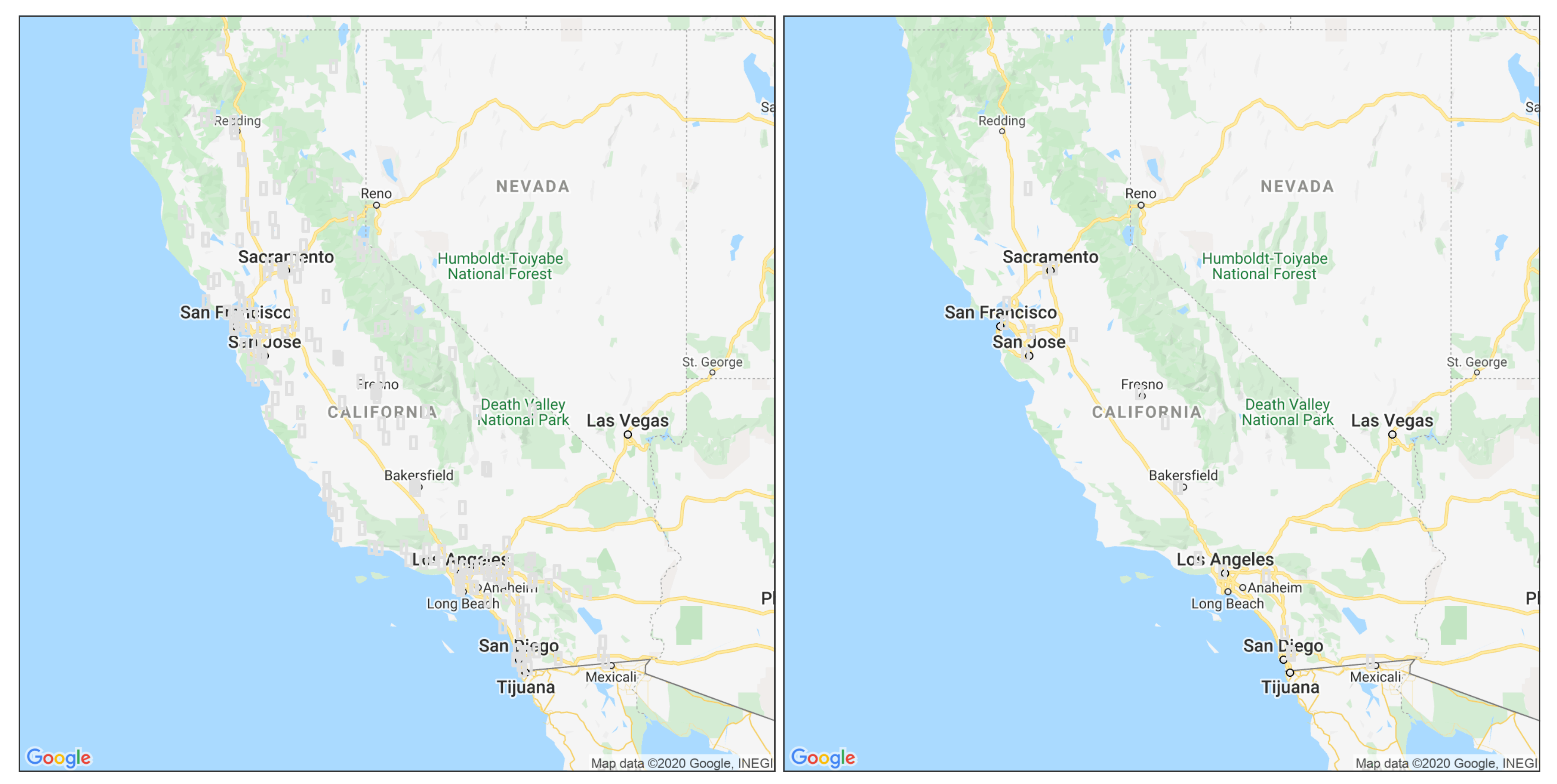
Map of the Children’s Health Study participants who were recruited in Santa Barbara (left) and other communities (right).
Figure 1.
Map of the Children’s Health Study participants who were recruited in Santa Barbara (left) and other communities (right).

Figure 2.
Relative importance of the ten most important features in model predicting PM using gradient boosting.
Figure 2.
Relative importance of the ten most important features in model predicting PM using gradient boosting.

Figure 3.
Relative importance of the ten most important features in models predicting SO (top left), NO (top right), EC (bottom left), and dust (bottom right). Feature importance were calculated using relative influences in GBM models (PM, SO, and EC) [44] and global sensitivity analysis in SVM models (NO and dust) [45]. SSR: surface shortwave radiation; ERC: energy release component.

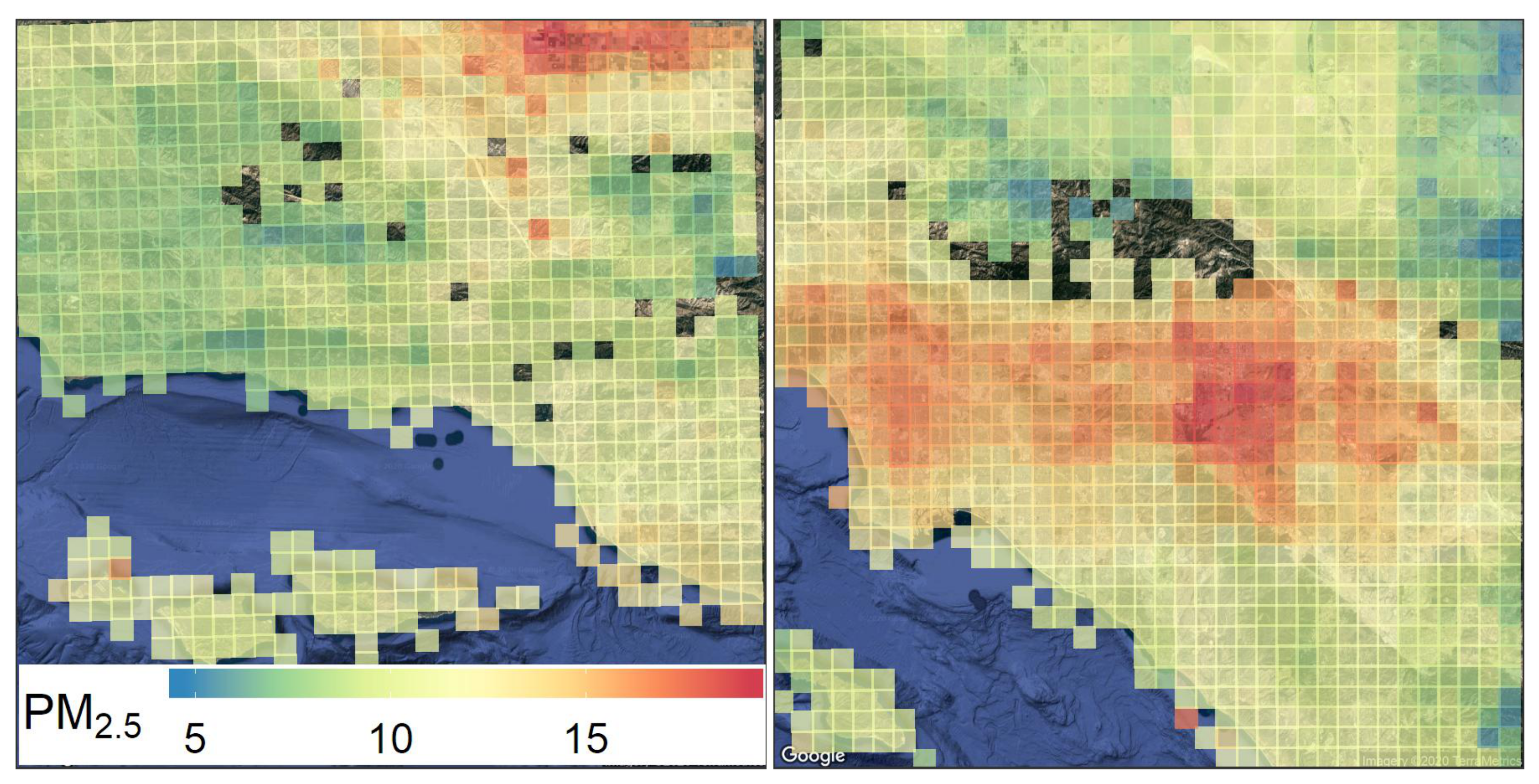
Figure 4.
Maps of mean MISR-derived PM (µg/m) from 2007 through 2012 over Santa Barbara (left) and other communities in Southern California (right).
Figure 4.
Maps of mean MISR-derived PM (µg/m) from 2007 through 2012 over Santa Barbara (left) and other communities in Southern California (right).

Figure 5.
Maps of mean MISR-derived SO (top left), NO (top right), EC (bottom left), and dust (bottom right) from 2007 through 2012, all measured in µg/m over Santa Barbara (left in each) and other communities in Southern California (right in each).
Figure 5.
Maps of mean MISR-derived SO (top left), NO (top right), EC (bottom left), and dust (bottom right) from 2007 through 2012, all measured in µg/m over Santa Barbara (left in each) and other communities in Southern California (right in each).

Table 1.
Summary of machine learning methods, MISR predictors, and best test R for predicting each exposure of interest.
Table 1.
Summary of machine learning methods, MISR predictors, and best test R for predicting each exposure of interest.
| Exposure | ML Method | MISR Predictors | Best Test R | Best Test RMSE (µg/m3) |
|---|---|---|---|---|
| PM | GBM | AOD Products | 0.68 | 4.75 |
| SO | GBM | AOD Products | 0.71 | 0.69 |
| NO | SVM | AOD Products | 0.71 | 2.13 |
| EC | GBM | AOD Products | 0.63 | 0.37 |
| Dust | SVM | AOD Mixtures | 0.53 | 0.60 |
Table 2.
Characteristics of the study population.
| Mean (SD) | N (%) | ||
|---|---|---|---|
| N | 1206 | Gender | |
| Lung function | Boys | 588 (48.8) | |
| Forced Vital Capacity (mL) | 4265 (856) | Girls | 618 (51.2) |
| Forced Expiratory Volume (mL) | 3700 (703) | Race/Ethnicity | |
| Exposures (µg/m3) | White | 413 (34.2) | |
| Central site | Asian | 54 (4.5) | |
| PM | 11.99 (2.9) | Black | 23 (1.9) |
| MISR-derived | Hispanic | 617 (51.2) | |
| PM | 14.22 (2.6) | Others | 99 (8.2) |
| Sulfate | 1.37 (0.3) | Community | |
| Nitrate | 2.36 (0.4) | Anaheim | 113 (9.4) |
| EC | 0.82 (0.1) | Glendora | 228 (18.9) |
| Dust | 1.12 (0.3) | Long Beach | 56 (4.6) |
| Demographics | Mira Loma | 146 (12.1) | |
| Age | 15.24 (0.6) | Riverside | 138 (11.4) |
| Height (cm) | 166.20 (8.6) | San Dimas | 170 (14.1) |
| Weight (kg) | 64.41 (15.8) | Santa Barbara | 186 (15.4) |
| BMI (kg/m) | 23.23 (5.0) | Upland | 169 (14.0) |
Table 3.
Air pollution single-pollutant effect estimates by outcome adjusted for demographic factors.
Table 3.
Air pollution single-pollutant effect estimates by outcome adjusted for demographic factors.
| FEV | FVC | ||||||
|---|---|---|---|---|---|---|---|
| Source | Exposure | Estimate * | 95% CI | p | Estimate * | 95% CI | p |
| Central site | PM | 0.521 | 0.775 | ||||
| MISR-derived | PM | 0.013 | 0.103 | ||||
| SO | 0.008 | 0.015 | |||||
| NO | 0.447 | 0.026 | |||||
| EC | 0.289 | 0.206 | |||||
| Dust | 0.011 | 0.316 | |||||
* Effect estimates are the difference in FEV and FVC from the highest to the lowest concentration of each air pollutant in µg/m: [Central sites] PM: 8.9; [MISR-derived] PM: 10.7, SO: 1.2, NO: 2.5, EC: 0.6, dust: 1.6.
© 2020 by the authors. Licensee MDPI, Basel, Switzerland. This article is an open access article distributed under the terms and conditions of the Creative Commons Attribution (CC BY) license (http://creativecommons.org/licenses/by/4.0/).
Share and Cite
MDPI and ACS Style
Chau, K.; Franklin, M.; Gauderman, W.J. Satellite-Derived PM2.5 Composition and Its Differential Effect on Children’s Lung Function. Remote Sens. 2020, 12, 1028. https://0-doi-org.brum.beds.ac.uk/10.3390/rs12061028
AMA Style
Chau K, Franklin M, Gauderman WJ. Satellite-Derived PM2.5 Composition and Its Differential Effect on Children’s Lung Function. Remote Sensing. 2020; 12(6):1028. https://0-doi-org.brum.beds.ac.uk/10.3390/rs12061028
Chicago/Turabian StyleChau, Khang, Meredith Franklin, and W. James Gauderman. 2020. "Satellite-Derived PM2.5 Composition and Its Differential Effect on Children’s Lung Function" Remote Sensing 12, no. 6: 1028. https://0-doi-org.brum.beds.ac.uk/10.3390/rs12061028
Note that from the first issue of 2016, this journal uses article numbers instead of page numbers. See further details here.