Nine-Year Systematic Evaluation of the GPM and TRMM Precipitation Products in the Shuaishui River Basin in East-Central China


Abstract
:
1. Introduction
2. Study Area
3. Materials and Methods
3.1. Satellite Precipitation Products
3.2. Ground Rainfall Measurements
3.3. Evaluation Metrics
3.4. Analysis of Variance (ANOVA)
4. Results and Discussions
4.1. Evaluation at the Monthly Scale
4.1.1. Temporal Analysis
4.1.2. Spatial Variation
4.2. Evaluation at the Daily Scale
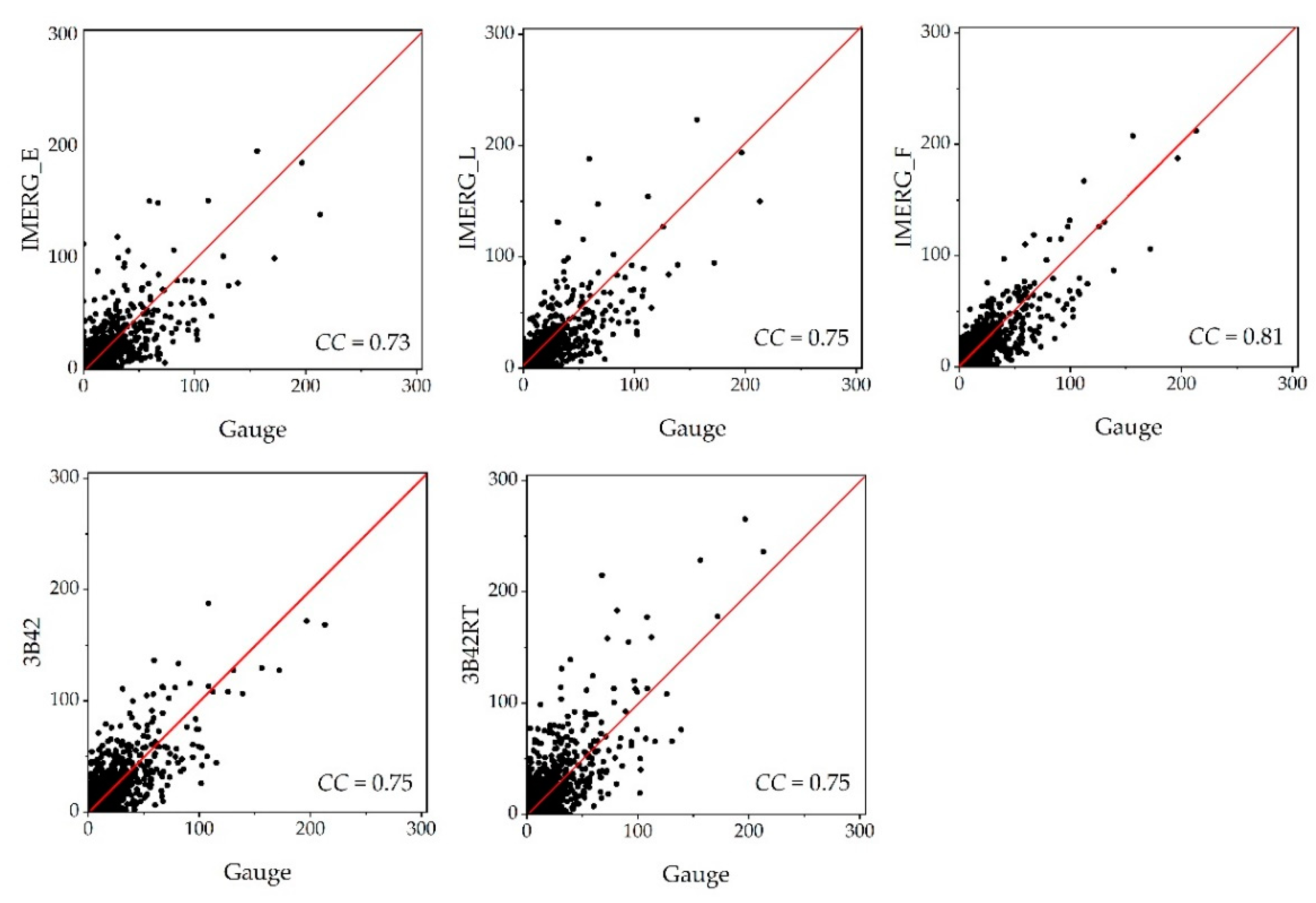
4.2.1. Continuous Evaluation Metrics
(1) Temporal Variation
(2) Statistical Performance Comparison among the SPPs
(3) Spatial Variation
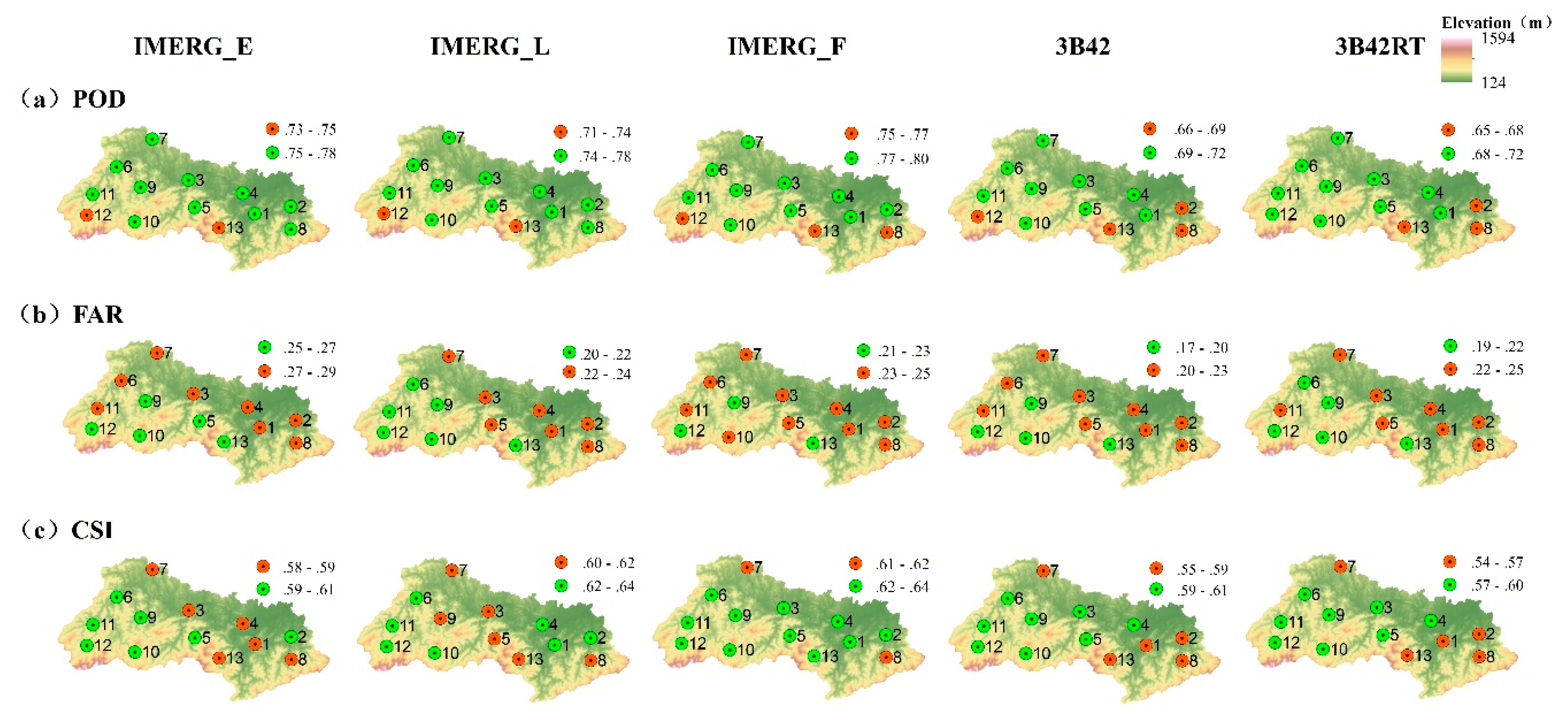
4.2.2. Categorical Evaluation Metrics
(1) Temporal Variation
(2) Spatial Variation
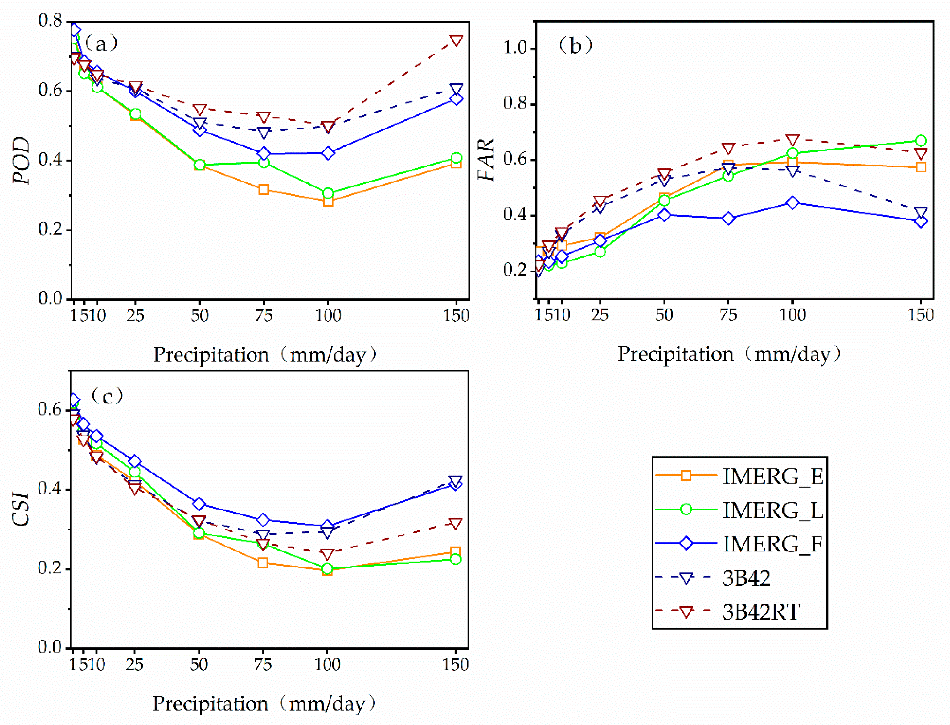
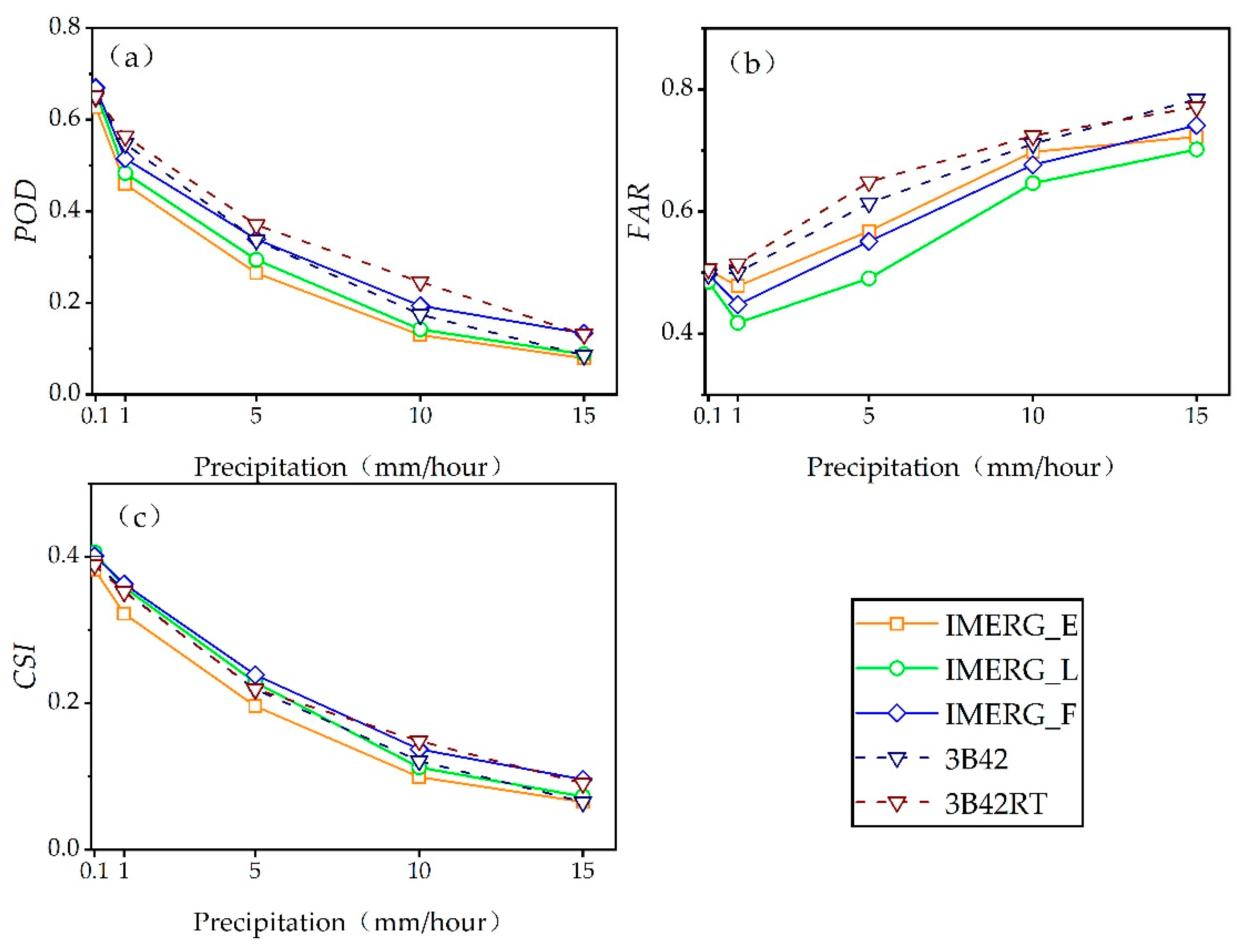
(3) Variation with Rainfall Thresholds
4.2.3. Comparison with Previous Studies
4.3. Evaluation at the Hourly Scale
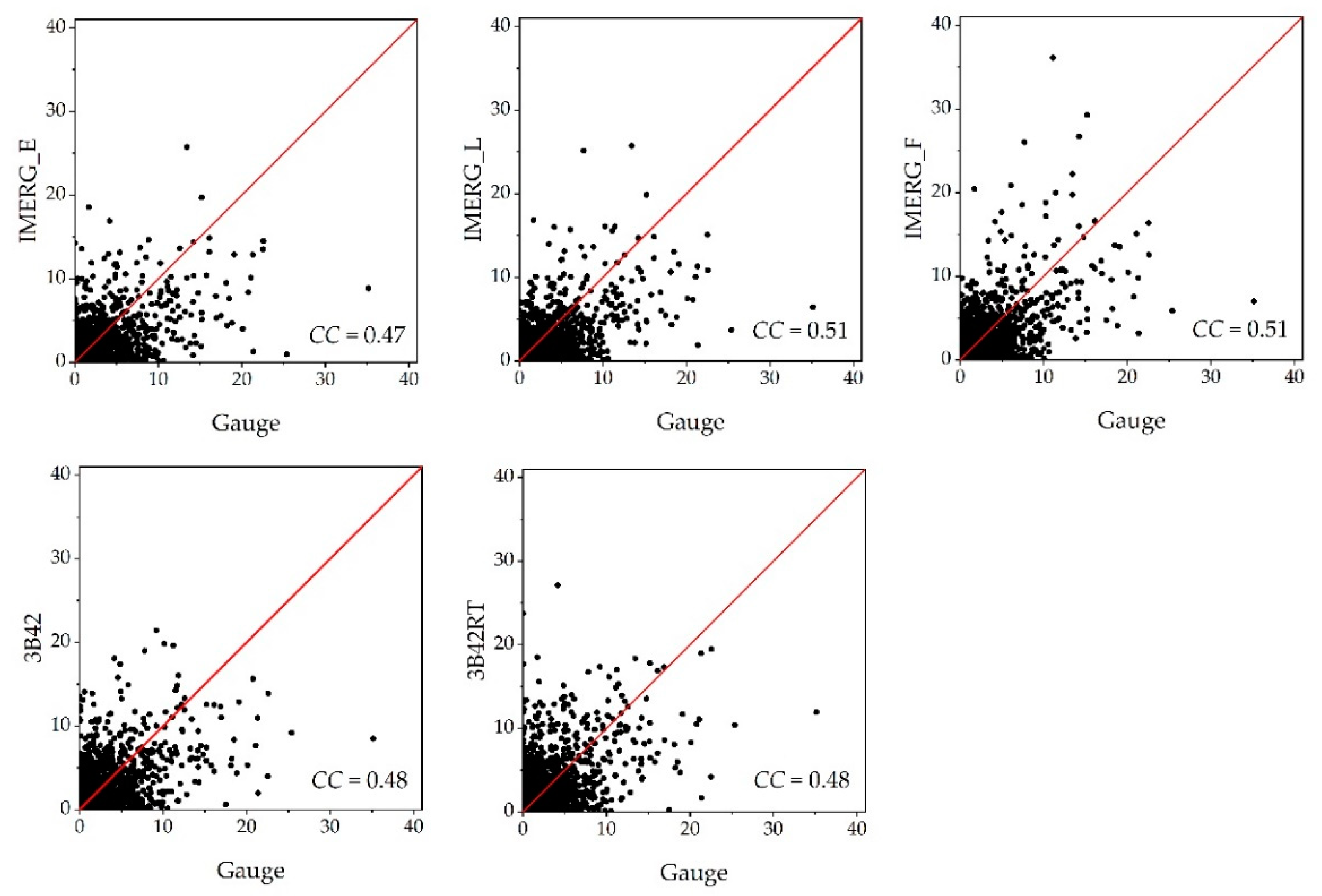
4.3.1. Continuous Evaluation Metrics
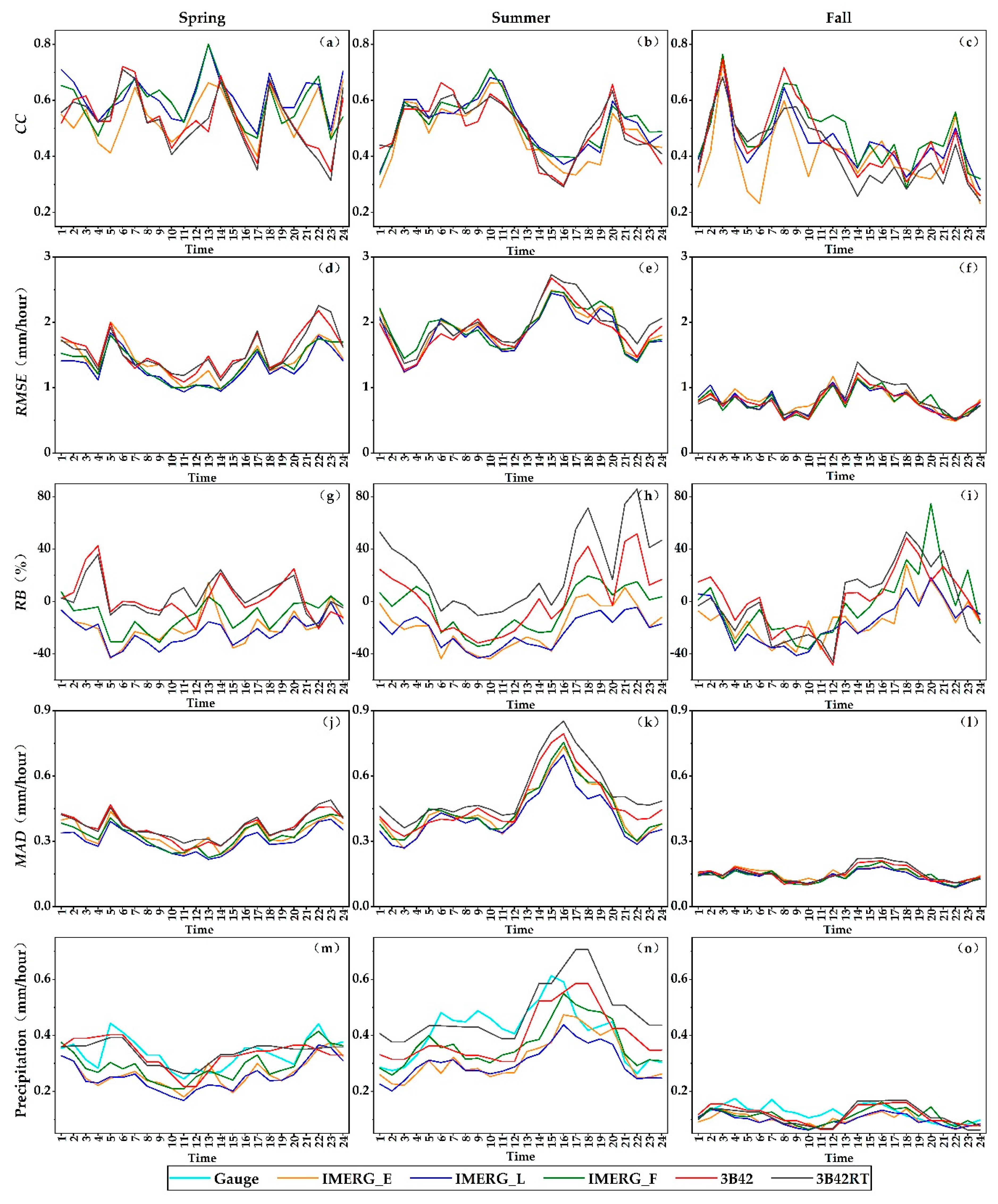
(1) Temporal Variation
(2) Statistical Performance Comparison among the SPPs
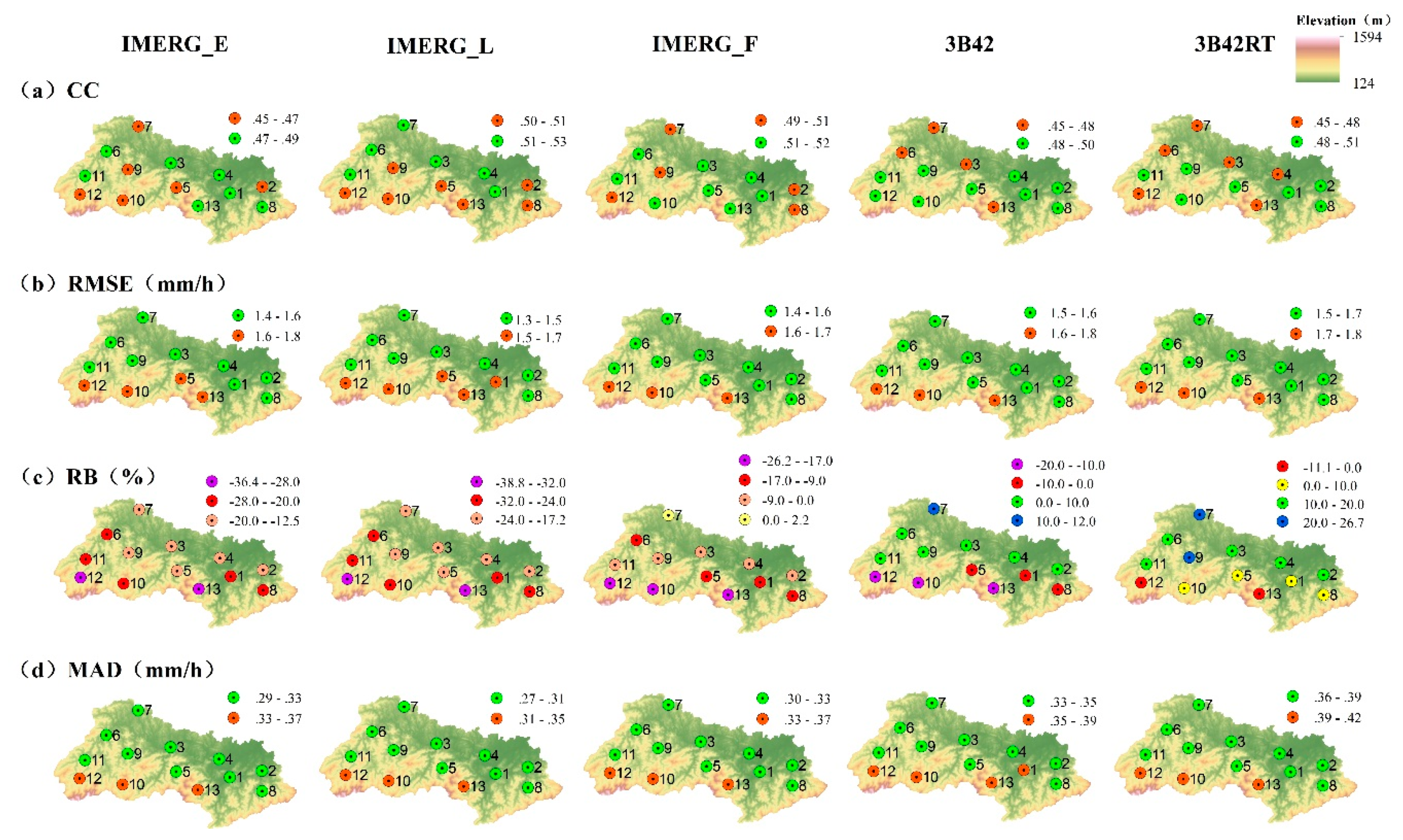
(3) Spatial Variation
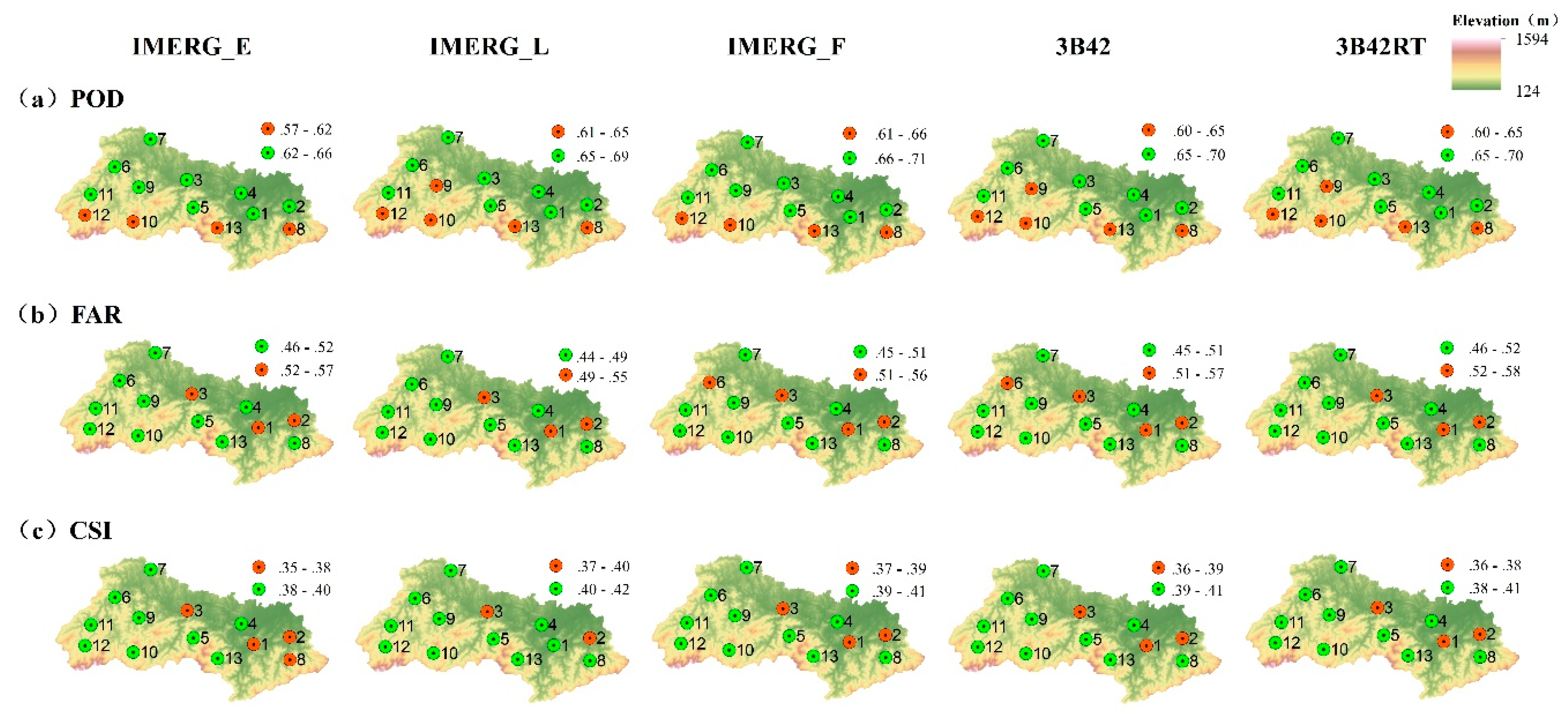
4.3.2. Categorical Evaluation Metrics
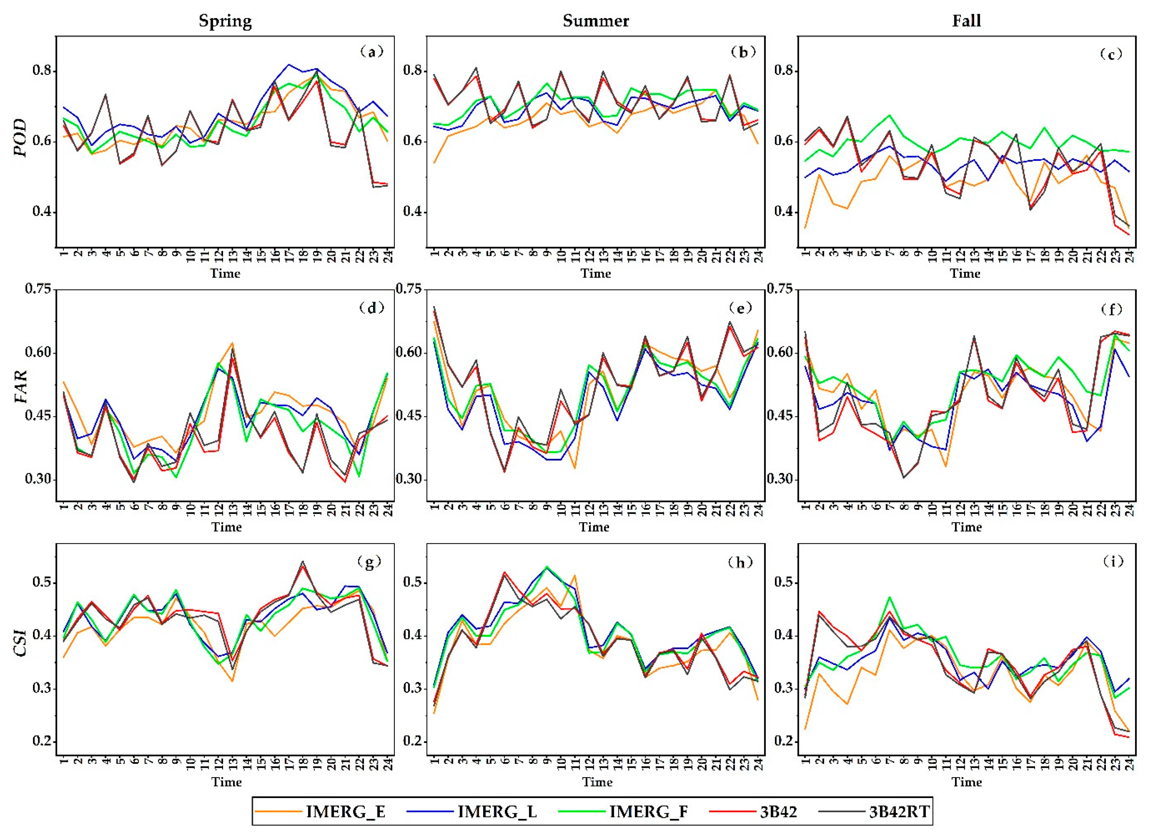
(1) Temporal Variation
(2) Spatial Variation
(3) Variation with Rainfall Thresholds
5. Conclusions
- (1)
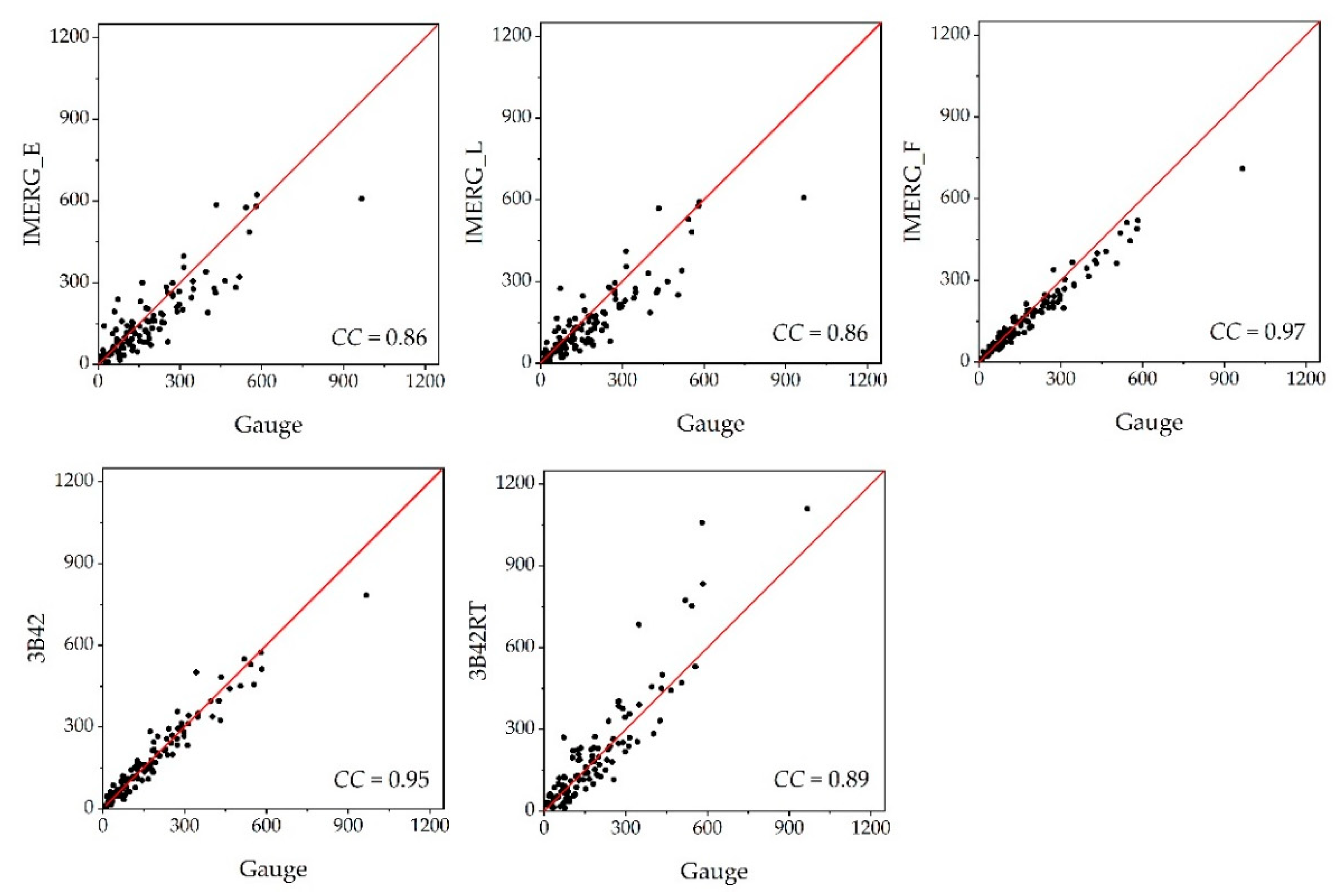
- Rainfall estimates by all five SPPs could match ground observations best at the monthly scale, followed by the daily and hourly scale. The annual CCs of the SPPs, for example, have fallen from 0.86 or above at the monthly scale to mostly around 0.75 at the daily scale, and sharply to less than 0.6 (April to October) at the hourly scale. Topography tends to impose similar impact on the performance of SPPs across various time scales, with more estimation deviations at high altitude.
- (2)
- For estimating monthly rainfall, IMERG_F performs the best, closely followed by 3B42. These two post-time SPPs produce considerably better monthly rainfall estimates than the rest real-time or near-real-time SPPs. All three IMERG products tend to underestimate monthly rainfall except a slight overestimation by the two near-real-time products in winter. Meanwhile, 3B42RT exhibits a strong tendency to overestimate in summer and winter.
- (3)
- For estimating daily rainfall, the IMERG products generally perform better than the TMPA products, with IMERG_F performing the best. Similar to the monthly scale, the IMERG family products tend to underestimate daily rainfall in all four seasons except the two near-real-time products in winter. In contrast, 3B42RT exhibits a strong tendency of overestimation in summer and winter. In terms of rainfall detection performance, the TMPA products are more capable of correctly detecting daily rainfall occurrences, while the IMERG products contain fewer false detections of rainfall occurrences.
- (4)
- For estimating hourly rainfall, the performance of the SPPs is much more homogeneous. Two IMERG products (IMERG_F and IMERG_L) have slightly outperformed the TMPA products for most of the time. All IMERG products tend to underestimate hourly rainfall throughout the three seasons between April and October. In contrast, 3B42RT shows a strong tendency of overestimation in summer. In addition, the performances of hourly rainfall detection are quite similar among the five SPPs.
Author Contributions
Funding
Conflicts of Interest
Appendix A


References
- Wu, P.; Christidis, N.; Stott, P. Anthropogenic impact on Earth’s hydrological cycle. Nat. Clim. Chang. 2013, 3, 807–810. [Google Scholar] [CrossRef]
- Allen, M.R.; Ingram, W.J. Constraints on future changes in climate and the hydrologic cycle. Nature 2012, 489, 590. [Google Scholar] [CrossRef] [Green Version]
- Lee, J.; Lee, E.-H.; Seol, K.-H. Validation of Integrated MultisatellitE Retrievals for GPM (IMERG. by using gauge-based analysis products of daily precipitation over East Asia. Theor. Appl. Climatol. 2019, 137, 2497–2512. [Google Scholar] [CrossRef]
- Hou, A.Y.; Kakar, R.K.; Neeck, S.; Azarbarzin, A.A.; Kummerow, C.D.; Kojima, M.; Oki, R.; Nakamura, K.; Iguchi, T. The global precipitation measurement mission. Bull. Am. Meteorol. Soc. 2014, 95, 701. [Google Scholar] [CrossRef]
- Shen, Y.; Xiong, A. Validation and comparison of a new gauge-based precipitation analysis over mainland China. Int. J. Climatol. 2016, 36, 252–265. [Google Scholar] [CrossRef]
- Tan, M.L.; Ibrahim, A.; Duan, Z.; Cracknell, A.P.; Chaplot, V. Evaluation of six high-resolution satellite and ground-based precipitation products over Malaysia. Remote Sens. 2015, 7, 1504–1528. [Google Scholar] [CrossRef] [Green Version]
- Tancreto, A.E. Comparison of Hydrologic Model Performance Statistics Using Thiessen Polygon Rain Gauge and NEXRAD Precipitation Input Methods at Different Watershed Spatial Scales and Rainfall Return Frequencies; University of North Florida: Jacksonville, FL, USA, 2015; Available online: https://digitalcommons.unf.edu/etd/584 (accessed on 23 March 2020).
- Louf, V.; Protat, A.; Warren, R.A.; Collis, S.M.; Wolff, D.B.; Raunyiar, S.; Jakob, C.; Petersen, W.A. An integrated approach to weather radar calibration and monitoring using ground clutter and satellite comparisons. J. Atmos. Ocean. Technol. 2019, 36, 17–39. [Google Scholar] [CrossRef] [Green Version]
- Letu, H.; Nagao, T.M.; Nakajima, T.Y.; Riedi, J.; Ishimoto, H.; Baran, A.J.; Shang, H.; Sekiguchi, M.; Kikuchi, M. Ice cloud properties from Himawari-8/AHI next-generation geostationary satellite: Capability of the AHI to monitor the DC cloud generation process. IEEE Trans. Geosci. Remote Sens. 2019, 57, 3229–3239. [Google Scholar] [CrossRef]
- Rutledge, S.A.; Chandrasekar, V.; Fuchs, B.; George, J.; Junyent, F.; Kennedy, P.; Dolan, B. Deployment of the SEA-POL C-band Polarimetric Radar to SPURS-2. Oceanography 2019, 32, 50–57. [Google Scholar] [CrossRef]
- Beck, H.E.; Pan, M.; Roy, T.; Weedon, G.P.; Pappenberger, F.; van Dijk, A.I.J.M.; Huffman, G.J.; Adler, R.F.; Wood, E.F. Daily evaluation of 26 precipitation datasets using Stage-IV gauge-radar data for the CONUS. Hydrol. Earth Syst. Sci. 2019, 23, 207–224. [Google Scholar] [CrossRef] [Green Version]
- Joss, J.; Waldvogel, A.; Collier, C.G. Precipitation Measurement and Hydrology. In Radar in Meteorology: Battan Memorial and 40th Anniversary Radar Meteorology Conference; Atlas, D., Ed.; American Meteorological Society: Boston, MA, USA, 1990; pp. 577–606. [Google Scholar] [CrossRef]
- Dinku, T.; Anagnostou, E.N.; Borga, M. Improving radar-based estimation of rainfall over complex terrain. J. Appl. Meteorol. 2002, 41, 1163–1178. [Google Scholar] [CrossRef]
- Funk, C.; Peterson, P.; Landsfeld, M.; Pedreros, D.; Verdin, J.; Shukla, S.; Husak, G.; Rowland, J.; Harrison, L.; Hoell, A.; et al. The climate hazards infrared precipitation with stations-a new environmental record for monitoring extremes. Sci. Data 2015, 2. [Google Scholar] [CrossRef] [Green Version]
- Guo, H.; Chen, S.; Bao, A.; Hu, J.; Gebregiorgis, A.S.; Xue, X.; Zhang, X. Inter-comparison of high-resolution satellite precipitation products over Central Asia. Remote Sens. 2015, 7, 7181–7211. [Google Scholar] [CrossRef] [Green Version]
- Mantas, V.M.; Liu, Z.; Caro, C.; Pereira, A.J.S.C. Validation of TRMM multi-satellite precipitation analysis (TMPA) products in the Peruvian Andes. Atmos. Res. 2015, 163, 132–145. [Google Scholar] [CrossRef]
- Li, X.-H.; Zhang, Q.; Xu, C.-Y. Suitability of the TRMM satellite rainfalls in driving a distributed hydrological model for water balance computations in Xinjiang catchment, Poyang lake basin. J. Hydrol. 2012, 426, 28–38. [Google Scholar] [CrossRef]
- Bharti, V.; Singh, C. Evaluation of error in TRMM 3B42V7 precipitation estimates over the Himalayan region. J. Geophys. Res. -Atmos. 2015, 120, 12458–12473. [Google Scholar] [CrossRef]
- Tan, M.L.; Duan, Z. Assessment of GPM and TRMM precipitation products over Singapore. Remote Sens. 2017, 9, 720. [Google Scholar] [CrossRef] [Green Version]
- Sharifi, E.; Steinacker, R.; Saghafian, B. Assessment of GPM-IMERG and other precipitation products against gauge data under different topographic and climatic conditions in Iran: Preliminary results. Remote Sens. 2016, 8, 135. [Google Scholar] [CrossRef] [Green Version]
- Tang, G.; Ma, Y.; Long, D.; Zhong, L.; Hong, Y. Evaluation of GPM Day-1 IMERG and TMPA Version-7 legacy products over Mainland China at multiple spatiotemporal scales. J. Hydrol. 2016, 533, 152–167. [Google Scholar] [CrossRef]
- Suratman, S.; Aziz, A.A.; Tahir, N.M.; Lee, L.H. Distribution and behaviour of nitrogen compounds in the surface water of Sungai Terengganu Estuary, Southern Waters of South China Sea, Malaysia. Sains Malays. 2018, 47, 651–659. [Google Scholar] [CrossRef]
- Zhou, Y.; Wu, T. Composite analysis of precipitation intensity and distribution characteristics of western track landfall typhoons over China under strong and weak monsoon conditions. Atmos. Res. 2019, 225, 131–143. [Google Scholar] [CrossRef]
- Yang, X.; Warren, R.; He, Y.; Ye, J.; Li, Q.; Wang, G. Impacts of climate change on TN load and its control in a river basin with complex pollution sources. Sci. Total Environ. 2018, 615, 1155–1163. [Google Scholar] [CrossRef] [Green Version]
- Yang, X.; Liu, Q.; Fu, G.; He, Y.; Luo, X.; Zheng, Z. Spatiotemporal patterns and source attribution of nitrogen load in a river basin with complex pollution sources. Water Res. 2016, 94, 187–199. [Google Scholar] [CrossRef] [Green Version]
- Boithias, L.; Sauvage, S.; Lenica, A.; Roux, H.; Abbaspour, K.C.; Larnier, K.; Dartus, D.; Sanchez-Perez, J.M. Simulating flash floods at hourly time-step using the SWAT model. Water 2017, 9, 929. [Google Scholar] [CrossRef] [Green Version]
- Zhou, M.M.; Deng, J.S.; Lin, Y.; Belete, M.; Wang, K.; Comber, A.; Huang, L.Y.; Gan, M.Y. Identifying the effects of land use change on sediment export: Integrating sediment source and sediment delivery in the Qiantang River Basin, China. Sci. Total Environ. 2019, 686, 38–49. [Google Scholar] [CrossRef]
- Lin, Q.W.; Peng, X.; Liu, B.Y.; Min, F.L.; Zhang, Y.; Zhou, Q.H.; Ma, J.M.; Wu, Z.B. Aluminum distribution heterogeneity and relationship with nitrogen, phosphorus and humic acid content in the eutrophic lake sediment. Environ. Pollut. 2019, 253, 516–524. [Google Scholar] [CrossRef]
- Wu, Y.; Zhang, Z.; Huang, Y.; Jin, Q.; Chen, X.; Chang, J. Evaluation of the GPM IMERG V5 and TRMM 3B42 V7 precipitation products in the Yangtze River Basin, China. Water 2019, 11, 1459. [Google Scholar] [CrossRef] [Green Version]
- Zhao, H.; Yang, S.; Wang, Z.; Zhou, X.; Luo, Y.; Wu, L. Evaluating the suitability of TRMM satellite rainfall data for hydrological simulation using a distributed hydrological model in the Weihe River catchment in China. J. Geogr. Sci. 2015, 25, 177–195. [Google Scholar] [CrossRef]
- Beaufort, A.; Gibier, F.; Palany, P. Assessment and correction of three satellite rainfall estimate products for improving flood prevention in French Guiana. Int. J. Remote Sens. 2019, 40, 171–196. [Google Scholar] [CrossRef]
- Huffman, G.J.; Adler, R.F.; Bolvin, D.T.; Gu, G.; Nelkin, E.J.; Bowman, K.P.; Hong, Y.; Stocker, E.F.; Wolff, D.B. The TRMM multisatellite precipitation analysis (TMPA): Quasi-global, multiyear, combined-sensor precipitation estimates at fine scales. J. Hydrometeorol. 2007, 8, 38–55. [Google Scholar] [CrossRef]
- Real-Time TRMM Multi-Satellite Precipitation Analysis Data Set Documentation. Available online: https://pmm.nasa.gov/sites/default/files/document_files/3B4XRT_doc_V7_180426.pdf (accessed on 17 March 2020).
- Bushair, M.T.; Kumar, P.; Gairola, R.M. Evaluation and assimilation of various satellite-derived rainfall products over India. Int. J. Remote Sens. 2019, 40, 5315–5338. [Google Scholar] [CrossRef]
- Algorithm Theoretical Basis Document (ATBD) Version 06. NASA Global Precipitation Measurement (GPM) Integrated Multi-satellitE Retrievals for GPM (IMERG). Available online: https://pmm.nasa.gov/sites/default/files/document_files/IMERG_ATBD_V06.pdf (accessed on 17 March 2020).
- Yong, B.; Ren, L.; Hong, Y.; Gourley, J.J.; Tian, Y.; Huffman, G.J.; Chen, X.; Wang, W.; Wen, Y. First evaluation of the climatological calibration algorithm in the real- time TMPA precipitation estimates over two basins at high and low latitudes. Water Resour. Res. 2013, 49, 2461–2472. [Google Scholar] [CrossRef] [Green Version]
- Condom, T.; Rau, P.; Espinoza, J.C. Correction of TRMM 3B43 monthly precipitation data over the mountainous areas of Peru during the period 1998–2007. Hydrol. Process. 2011, 25, 1924–1933. [Google Scholar] [CrossRef]
- Blacutt, L.A.; Herdies, D.L.; de Goncalves, L.G.G.; Vila, D.A.; Andrade, M. Precipitation comparison for the CFSR, MERRA, TRMM3B42 and Combined Scheme datasets in Bolivia. Atmos. Res. 2015, 163, 117–131. [Google Scholar] [CrossRef] [Green Version]
- El Kenawy, A.M.; Lopez-Moreno, J.I.; McCabe, M.F.; Vicente-Serrano, S.M. Evaluation of the TMPA-3B42 precipitation product using a high-density rain gauge network over complex terrain in northeastern Iberia. Glob. Planet. Chang. 2015, 133, 188–200. [Google Scholar] [CrossRef] [Green Version]
- Yong, B.; Ren, L.-L.; Hong, Y.; Wang, J.-H.; Gourley, J.J.; Jiang, S.-H.; Chen, X.; Wang, W. Hydrologic evaluation of multisatellite precipitation analysis standard precipitation products in basins beyond its inclined latitude band: A case study in Laohahe basin, China. Water Resour. Res. 2010, 46. [Google Scholar] [CrossRef] [Green Version]
- Gerapetritis, H.; Pelissier, J. The critical success index and warning strategy. In Proceedings of the 17th Conference on Probablity and Statistics in the Atmospheric Sciences, Seattle, WC, USA, 11–15 January 2004. [Google Scholar]
- Chen, S.; Hong, Y.; Cao, Q.; Gourley, J.J.; Kirstetter, P.-E.; Yong, B.; Tian, Y.; Zhang, Z.; Shen, Y.; Hu, J.; et al. Similarity and difference of the two successive V6 and V7 TRMM multisatellite precipitation analysis performance over China. J. Geophys. Res. -Atmos. 2013, 118, 13060–13074. [Google Scholar] [CrossRef]
- Anjum, M.N.; Ding, Y.; Shangguan, D.; Ahmad, I.; Ijaz, M.W.; Farid, H.U.; Yagoub, Y.E.; Zaman, M.; Adnan, M. Performance evaluation of latest integrated multi-satellite retrievals for Global Precipitation Measurement (IMERG) over the northern highlands of Pakistan. Atmos. Res. 2018, 205, 134–146. [Google Scholar] [CrossRef]
- Yang, M.; Li, Z.; Anjum, M.N.; Gao, Y. Performance Evaluation of Version 5 (V05) of Integrated Multi-Satellite Retrievals for Global Precipitation Measurement (IMERG) over the Tianshan Mountains of China. Water 2019, 11, 1139. [Google Scholar] [CrossRef] [Green Version]
- Milewski, A.; Elkadiri, R.; Durham, M. Assessment and comparison of TMPA satellite precipitation products in varying climatic and topographic regimes in Morocco. Remote Sens. 2015, 7, 5697–5717. [Google Scholar] [CrossRef] [Green Version]
- Su, J.; Lu, H.; Zhu, Y.; Cui, Y.; Wang, X. Evaluating the hydrological utility of latest IMERG products over the Upper Huaihe River Basin, China. Atmos. Res. 2019, 225, 17–29. [Google Scholar] [CrossRef]
- Wang, X.; Ding, Y.; Zhao, C.; Wang, J. Similarities and improvements of GPM IMERG upon TRMM 3B42 precipitation product under complex topographic and climatic conditions over Hexi region, Northeastern Tibetan Plateau. Atmos. Res. 2019, 218, 347–363. [Google Scholar] [CrossRef]
- Xu, F.; Guo, B.; Ye, B.; Ye, Q.; Chen, H.; Ju, X.; Guo, J.; Wang, Z. Systematical Evaluation of GPM IMERG and TRMM 3B42V7 Precipitation Products in the Huang-Huai-Hai Plain, China. Remote Sens. 2019, 11, 697. [Google Scholar] [CrossRef] [Green Version]
- Tan, M.L.; Santo, H. Comparison of GPM IMERG, TMPA 3B42 and PERSIANN-CDR satellite precipitation products over Malaysia. Atmos. Res. 2018, 202, 63–76. [Google Scholar] [CrossRef]
- Aslami, F.; Ghorbani, A.; Sobhani, B.; Esmali, A. Comprehensive comparison of daily IMERG and GSMaP satellite precipitation products in Ardabil Province, Iran. Int. J. Remote Sens. 2019, 40, 3139–3153. [Google Scholar] [CrossRef]
- Kim, K.; Park, J.; Baik, J.; Choi, M. Evaluation of topographical and seasonal feature using GPM IMERG and TRMM 3B42 over Far-East Asia. Atmos. Res. 2017, 187, 95–105. [Google Scholar] [CrossRef]
- Wang, W.; Lu, H.; Zhao, T.; Jiang, L.; Shi, J. Evaluation and comparison of daily rainfall from latest GPM and TRMM products over the Mekong River Basin. IEEE J. Sel. Top. Appl. Earth Obs. Remote Sens. 2017, 10, 2540–2549. [Google Scholar] [CrossRef]
- Caracciolo, D.; Francipane, A.; Viola, F.; Noto, L.V.; Deidda, R. Performances of GPM satellite precipitation over the two major Mediterranean islands. Atmos. Res. 2018, 213, 309–322. [Google Scholar] [CrossRef] [Green Version]
- Li, N.; Tang, G.; Zhao, P.; Hong, Y.; Gou, Y.; Yang, K. Statistical assessment and hydrological utility of the latest multi-satellite precipitation analysis IMERG in Ganjiang River basin. Atmos. Res. 2017, 183, 212–223. [Google Scholar] [CrossRef]
- Yuan, F.; Zhang, L.; Soe, K.M.W.; Ren, L.; Zhao, C.; Zhu, Y.; Jiang, S.; Liu, Y. Applications of TRMM- and GPM-Era multiple-satellite precipitation products for flood simulations at sub-daily scales in a sparsely gauged watershed in Myanmar. Remote Sens. 2019, 11, 140. [Google Scholar] [CrossRef] [Green Version]
- Omranian, E.; Sharif, H.O. Evaluation of the Global Precipitation Measurement (GPM) satellite rainfall products over the Lower Colorado River Basin, Texas. J. Am. Water Resour. Assoc. 2018, 54, 882–898. [Google Scholar] [CrossRef]


| SPPs Estimates | Rain Gauge Observations | |
|---|---|---|
| S ≥ Threshold | S < Threshold | |
| P ≥ Threshold | H | F |
| P < Threshold | M | Z |
| Metrics | Temporal Scale | IMERG_E | IMERG_L | IMERG_F | 3B42 | 3B42RT |
|---|---|---|---|---|---|---|
| CC | Annual | 0.86 | 0.86 | 0.97 | 0.95 | 0.89 |
| Spring a | 0.72 | 0.77 | 0.95 | 0.93 | 0.82 | |
| Summer a | 0.89 | 0.90 | 0.95 | 0.93 | 0.89 | |
| Fall a | 0.65 | 0.69 | 0.88 | 0.83 | 0.74 | |
| Winter a | 0.69 | 0.70 | 0.98 | 0.97 | 0.81 | |
| RMSE (mm) | Annual | 86.69 | 87.64 | 53.82 | 54.13 | 101.42 |
| Spring | 90.17 | 89.50 | 47.23 | 44.02 | 75.09 | |
| Summer | 118.98 | 121.71 | 87.19 | 87.36 | 170.08 | |
| Fall | 53.88 | 52.51 | 30.64 | 35.79 | 49.90 | |
| Winter | 67.13 | 68.93 | 25.18 | 26.41 | 61.58 | |
| RB (%) | Annual | −13.63 | −16.80 | −10.51 | 0.61 | 10.69 |
| Spring | −13.74 | −19.33 | −12.00 | −0.02 | −4.91 | |
| Summer | −19.13 | −22.71 | −9.85 | −1.48 | 25.77 | |
| Fall | −11.20 | −9.84 | −6.35 | 0.12 | −3.89 | |
| Winter | 0.79 | 0.15 | −11.88 | 9.68 | 19.06 | |
| MAD (mm) | Annual | 61.59 | 61.77 | 35.79 | 37.07 | 65.72 |
| Spring | 71.80 | 70.72 | 37.99 | 34.34 | 60.64 | |
| Summer | 84.78 | 87.90 | 65.17 | 65.30 | 118.77 | |
| Fall | 43.50 | 41.97 | 23.17 | 28.40 | 40.75 | |
| Winter | 46.28 | 46.48 | 16.83 | 20.25 | 42.74 |
| Metrics | Temporal Scale | IMERG_E | IMERG_L | IMERG_F | 3B42 | 3B42RT |
|---|---|---|---|---|---|---|
| CC | Annual | 0.73 | 0.75 | 0.81 | 0.75 | 0.75 |
| Spring a | 0.71 | 0.77 | 0.79 | 0.74 | 0.73 | |
| Summer a | 0.80 | 0.81 | 0.83 | 0.78 | 0.77 | |
| Fall a | 0.64 | 0.65 | 0.73 | 0.70 | 0.68 | |
| Winter a | 0.66 | 0.66 | 0.82 | 0.72 | 0.68 | |
| RMSE (mm) | Annual | 11.30 | 11.07 | 9.66 | 11.54 | 12.96 |
| Spring | 12.23 | 11.04 | 10.61 | 13.20 | 13.05 | |
| Summer | 14.52 | 14.15 | 13.74 | 15.04 | 18.55 | |
| Fall | 8.03 | 8.56 | 6.67 | 7.56 | 7.82 | |
| Winter | 9.03 | 9.48 | 5.36 | 8.43 | 9.66 | |
| RB (%) | Annual | −13.15 | −16.33 | −9.99 | 1.21 | 11.36 |
| Spring | −11.89 | −17.62 | −11.55 | 0.47 | −4.43 | |
| Summer | −16.96 | −20.62 | −7.51 | −0.59 | 26.94 | |
| Fall | −9.68 | −8.06 | −4.31 | 0.56 | -3.47 | |
| Winter | 2.98 | 2.23 | −9.88 | 9.57 | 18.94 | |
| MAD (mm) | Annual | 4.52 | 4.19 | 4.00 | 4.77 | 5.21 |
| Spring | 5.45 | 4.81 | 4.90 | 5.81 | 5.71 | |
| Summer | 6.72 | 6.27 | 6.37 | 7.12 | 8.53 | |
| Fall | 2.93 | 2.85 | 2.60 | 2.91 | 2.98 | |
| Winter | 2.98 | 2.85 | 2.19 | 3.19 | 3.55 |
| Metrics | Temporal Scale | IMERG_E | IMERG_L | IMERG_F | 3B42 | 3B42RT |
|---|---|---|---|---|---|---|
| POD | Annual | 0.76 | 0.75 | 0.78 | 0.70 | 0.70 |
| Spring a | 0.87 | 0.86 | 0.85 | 0.76 | 0.75 | |
| Summer a | 0.82 | 0.79 | 0.83 | 0.82 | 0.82 | |
| Fall a | 0.65 | 0.65 | 0.72 | 0.60 | 0.60 | |
| Winter a | 0.65 | 0.66 | 0.67 | 0.44 | 0.41 | |
| FAR | Annual | 0.27 | 0.22 | 0.23 | 0.21 | 0.23 |
| Spring | 0.23 | 0.17 | 0.19 | 0.12 | 0.12 | |
| Summer | 0.32 | 0.27 | 0.29 | 0.24 | 0.24 | |
| Fall | 0.31 | 0.27 | 0.28 | 0.21 | 0.21 | |
| Winter | 0.24 | 0.19 | 0.17 | 0.09 | 0.12 | |
| CSI | Annual | 0.59 | 0.62 | 0.63 | 0.59 | 0.58 |
| Spring | 0.69 | 0.73 | 0.71 | 0.69 | 0.68 | |
| Summer | 0.59 | 0.61 | 0.62 | 0.65 | 0.65 | |
| Fall | 0.50 | 0.52 | 0.56 | 0.52 | 0.52 | |
| Winter | 0.54 | 0.57 | 0.59 | 0.42 | 0.39 |
| Study | Region | Study Area | Period | IMERG Products | TMPA Products | ||||||||||||
|---|---|---|---|---|---|---|---|---|---|---|---|---|---|---|---|---|---|
| CC | RMSE (mm/d) | RB(%) | MAD (mm/d) | POD | FAR | CSI | CC | RMSE (mm/d) | RB (%) | MAD (mm/d) | POD | FAR | CSI | ||||
| This study | Shuaishui River Basin, China | 1.5 × 10³ km2 | 2009.1–2017.12 | 0.73–0.81 | 9.66–11.07 | −16.33–−9.99 | 4.00–4.52 | 0.75–0.78 | 0.22–0.27 | 0.59–0.63 | 0.75 | 11.54–12.96 | 1.21–11.36 | 4.77–5.21 | 0.70 | 0.21–0.23 | 0.58–0.59 |
| Anjum et al. [43] | Northern Highlands, Pakistan | NA | 2014.4–2016.12 | 0.63 | 1.77 | 7.04 | / | 0.72 | 0.24 | 0.54 | 0.70 | 1.85 | 14.77 | / | 0.66 | 0.28 | 0.52 |
| Aslami et al. [50] | Ardabil Province, Iran | 1.8 × 10⁶ km2 | 2016.1–2017.10 | 0.33 | 0.83 | 24.46 | 0.10 | 0.91 | 0.16 | 0.78 | / | / | / | / | / | / | / |
| Beaufort et al. [31] | French Guiana | 8.6 × 10⁴ km2 | 2015.4–2016.3 | / | 13.80 | −3.10 | 7.40 | 0.70 | 0.36 | / | / | 14.40 | −3.30 | 8.40 | 0.30 | 0.35 | / |
| Kim et al. [51] | Japan | 3.8 × 10⁵ km2 | 2014.3–2014.8 | / | 18.77 | / | 6.16 | 0.68 | 0.20 | 0.58 | / | 20.29 | / | 6.70 | 0.62 | 0.29 | 0.49 |
| Sharifi et al. [20] | Several Provinces, Iran | 6.4 × 10⁴ km2 | 2014.3–2015.2 | 0.40–0.52 | 6.38–19.41 | −0.37–0.10 | 4.42–11.59 | 0.46–0.70 | 0.43–0.59 | 0.29–0.42 | 0.27–0.47 | 7.64–19.59 | −9.75–−1.47 | 5.39–11.68 | 0.39–0.56 | 0.55–0.71 | 0.23–0.33 |
| Su et al. [46] | Huaihe River Basin, China | 1.6 × 10⁴ km2 | 2014.4–2015.12 | 0.82–0.87 | 4.31–5.15 | 7.99–9.41 | / | 0.82– 0.83 | 0.31–0.38 | 0.55–0.60 | / | / | / | / | / | / | / |
| Tan et al. [19] | Singapore | 720 km2 | 2014.4–2016.6 | 0.53 | 11.83 | 5.24 | / | 0.78 | 0.28 | 0.60 | 0.56 | 9.20 | −10.25 | / | 0.66 | 0.15 | 0.65 |
| Tan et al. [49] | Malaysia | 3.3 × 10⁴ km2 | 2014.3–2016.2 | 0.50–0.60 | 12.94–14.93 | 13.24 | / | 0.86–0.89 | 0.18–0.20 | 0.73–0.74 | 0.57 | 13.60 | 9.98 | / | 0.85 | 0.15 | 0.74 |
| Wang et al. [52] | Mekong River Basin | 7.95 × 10⁵ km2 | 2014.4–2016.1 | 0.58 | 2.24 | −0.084 | / | 0.73 | 0.22 | 0.61 | 0.44 | 2.52 | −0.10 | / | 0.65 | 0.25 | 0.53 |
| Wu et al. [29] | Yangtze River Basin, China | 1.8 × 10⁶ km2 | 2014.4–2017.12 | 0.44 | 11.42 | 5.39 | 4.43 | / | / | / | 0.46 | 10.75 | 2.87 | 4.10 | / | / | / |
| Metrics | Temporal Scale | IMERG_E | IMERG_L | IMERG_F | 3B42 | 3B42RT |
|---|---|---|---|---|---|---|
| CC | Apr. to Oct. | 0.47 | 0.51 | 0.51 | 0.48 | 0.48 |
| Spring a | 0.53 | 0.60 | 0.58 | 0.52 | 0.51 | |
| Summer a | 0.46 | 0.49 | 0.49 | 0.47 | 0.48 | |
| Fall a | 0.35 | 0.38 | 0.41 | 0.40 | 0.36 | |
| RMSE (mm) | Apr. to Oct. | 1.57 | 1.51 | 1.56 | 1.60 | 1.65 |
| Spring | 1.47 | 1.36 | 1.41 | 1.59 | 1.58 | |
| Summer | 1.94 | 1.89 | 1.97 | 1.94 | 2.03 | |
| Fall | 0.89 | 0.88 | 0.86 | 0.86 | 0.90 | |
| RB (%) | Apr. to Oct. | −22.18 | −25.06 | −10.31 | −1.85 | 10.16 |
| Spring | −21.33 | −24.61 | −12.27 | 0.11 | 1.42 | |
| Summer | −22.98 | −26.08 | −9.26 | −2.20 | 18.35 | |
| Fall | −20.19 | −20.94 | −9.77 | −5.06 | −7.17 | |
| MAD(mm) | Apr. to Oct. | 0.33 | 0.31 | 0.33 | 0.35 | 0.37 |
| Spring | 0.33 | 0.30 | 0.33 | 0.36 | 0.37 | |
| Summer | 0.44 | 0.42 | 0.45 | 0.48 | 0.52 | |
| Fall | 0.15 | 0.14 | 0.14 | 0.15 | 0.15 |
| Metrics | Temporal Scale | IMERG_E | IMERG_L | IMERG_F | 3B42 | 3B42RT |
|---|---|---|---|---|---|---|
| POD | Apr. to Oct. | 0.63 | 0.66 | 0.67 | 0.65 | 0.65 |
| Spring a | 0.65 | 0.68 | 0.65 | 0.63 | 0.63 | |
| Summer a | 0.66 | 0.69 | 0.71 | 0.71 | 0.71 | |
| Fall a | 0.49 | 0.54 | 0.60 | 0.53 | 0.54 | |
| FAR | Apr. to Oct. | 0.50 | 0.49 | 0.50 | 0.50 | 0.51 |
| Spring | 0.46 | 0.45 | 0.43 | 0.40 | 0.41 | |
| Summer | 0.53 | 0.50 | 0.52 | 0.54 | 0.55 | |
| Fall | 0.51 | 0.49 | 0.53 | 0.50 | 0.51 | |
| CSI | Apr. to Oct. | 0.38 | 0.41 | 0.40 | 0.39 | 0.39 |
| Spring | 0.42 | 0.44 | 0.43 | 0.44 | 0.43 | |
| Summer | 0.38 | 0.41 | 0.40 | 0.38 | 0.38 | |
| Fall | 0.32 | 0.35 | 0.36 | 0.35 | 0.35 |
© 2020 by the authors. Licensee MDPI, Basel, Switzerland. This article is an open access article distributed under the terms and conditions of the Creative Commons Attribution (CC BY) license (http://creativecommons.org/licenses/by/4.0/).
Share and Cite
Yang, X.; Lu, Y.; Tan, M.L.; Li, X.; Wang, G.; He, R. Nine-Year Systematic Evaluation of the GPM and TRMM Precipitation Products in the Shuaishui River Basin in East-Central China. Remote Sens. 2020, 12, 1042. https://0-doi-org.brum.beds.ac.uk/10.3390/rs12061042
Yang X, Lu Y, Tan ML, Li X, Wang G, He R. Nine-Year Systematic Evaluation of the GPM and TRMM Precipitation Products in the Shuaishui River Basin in East-Central China. Remote Sensing. 2020; 12(6):1042. https://0-doi-org.brum.beds.ac.uk/10.3390/rs12061042
Chicago/Turabian StyleYang, Xiaoying, Yang Lu, Mou Leong Tan, Xiaogang Li, Guoqing Wang, and Ruimin He. 2020. "Nine-Year Systematic Evaluation of the GPM and TRMM Precipitation Products in the Shuaishui River Basin in East-Central China" Remote Sensing 12, no. 6: 1042. https://0-doi-org.brum.beds.ac.uk/10.3390/rs12061042