Mapping Kenyan Grassland Heights Across Large Spatial Scales with Combined Optical and Radar Satellite Imagery

 ,
,
Abstract
:
1. Introduction
2. Background
3. Methods
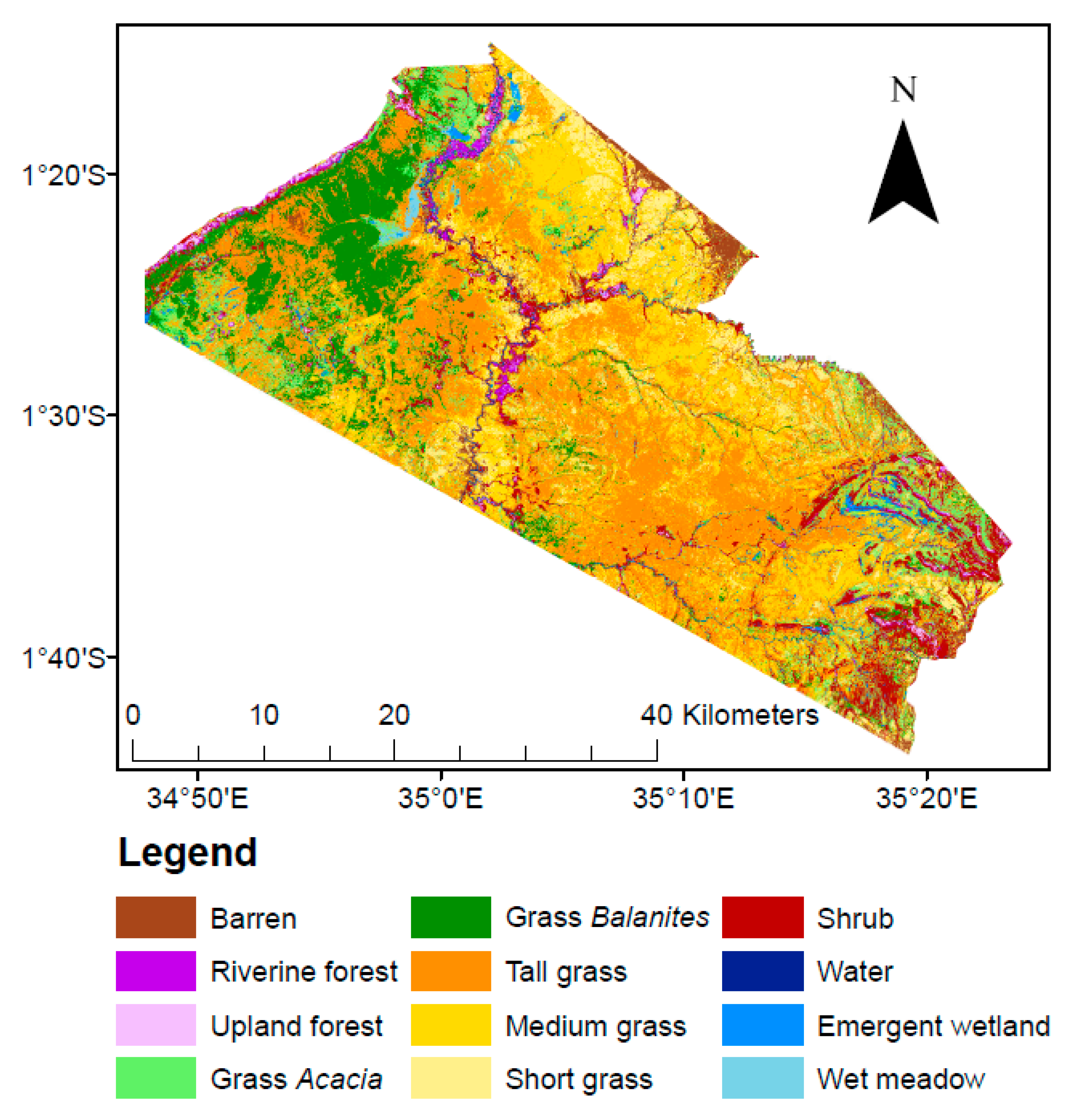
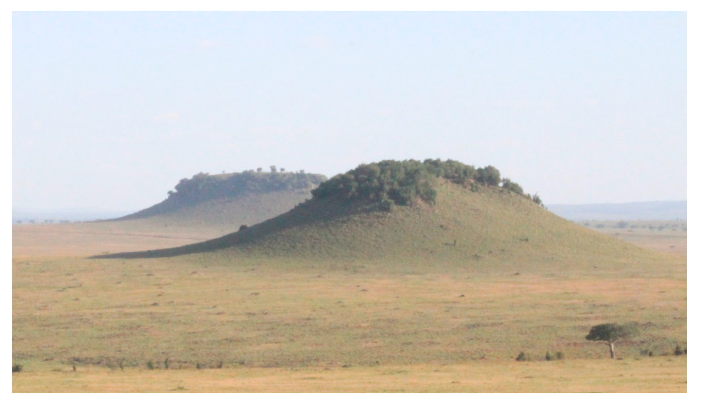
3.1. Study Area
3.2. Remote Sensing Data
3.2.1. ALOS-2 PALSAR-2 Radar Imagery
3.2.2. Sentinel Radar and Optical Imagery
3.3. Training and Validation Data
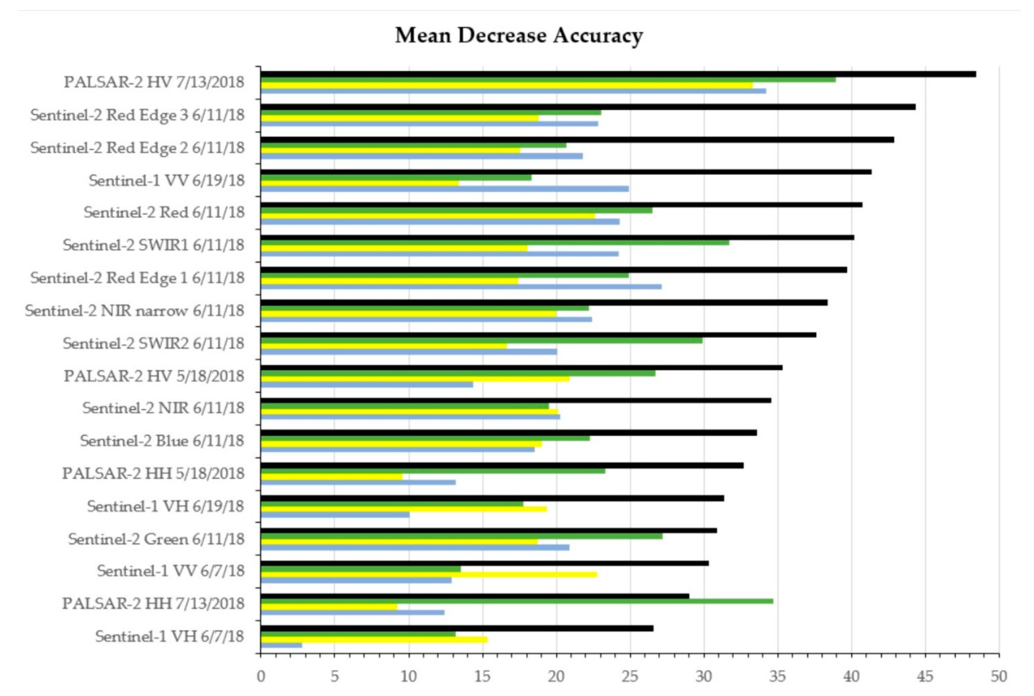
3.4. Supervised Land Cover Classification
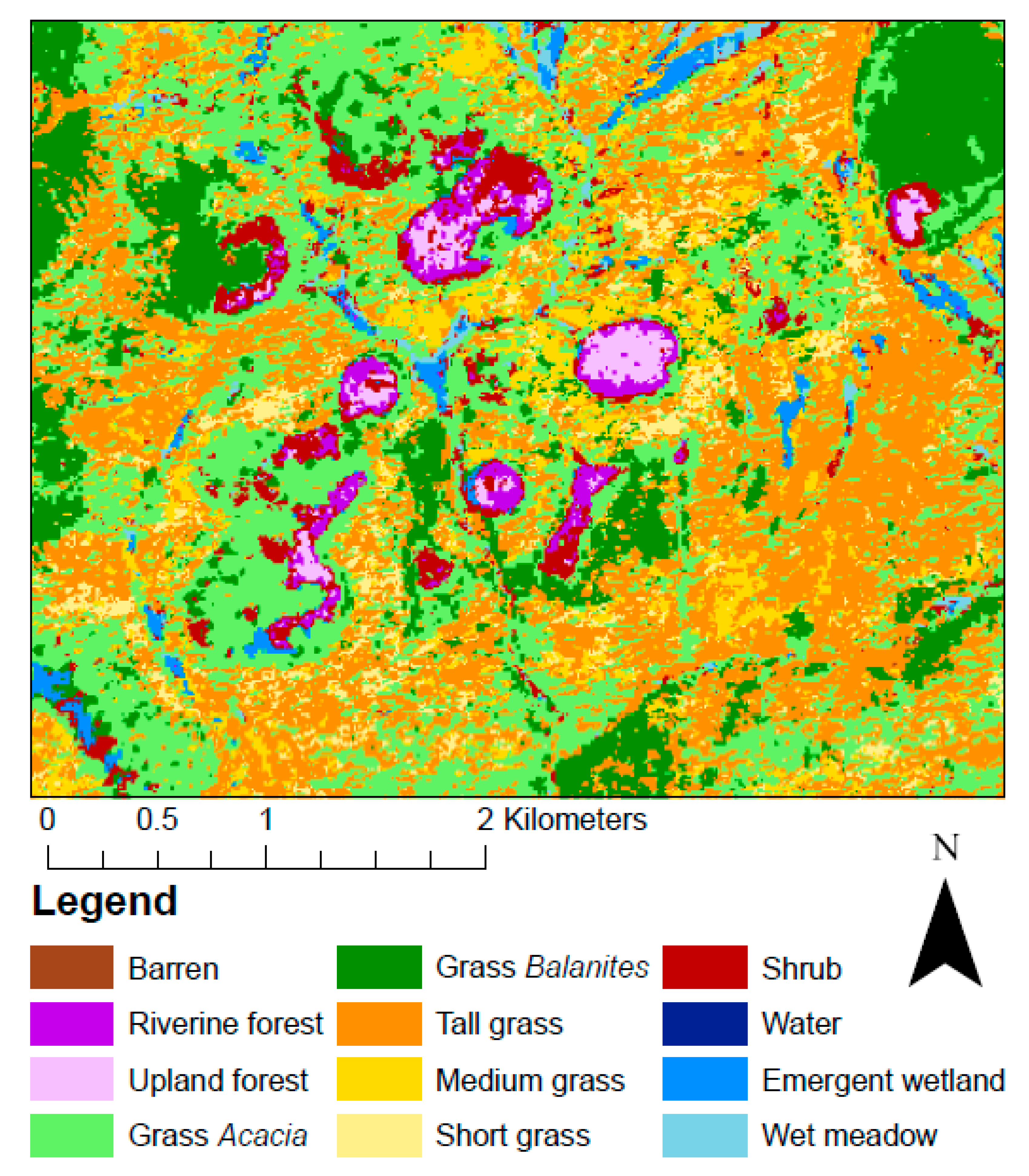
4. Results
5. Discussion
6. Conclusions
Supplementary Materials
Author Contributions
Funding
Acknowledgments
Conflicts of Interest
References
- Lieth, H.F.H. (Ed.) Patterns of Primary Productivity in the Biosphere; Hutchinson Ross: Stroudsberg, PA, USA, 1978. [Google Scholar]
- O’Mara, F.P. The role of grasslands in food security and climate change. Ann. Bot. 2012, 110, 1263–1270. [Google Scholar] [CrossRef] [Green Version]
- Scurlock, J.M.O.; Hall, D.O. The global carbon sink: A grassland perspective. Glob. Chang. Biol. 1998, 4, 229–233. [Google Scholar] [CrossRef] [Green Version]
- Bazilevich, N.I.; Rodin, L.Y. Geographical regularities in productivity and the circulation of chemical elements in the earth’s main vegetation types. Sov. Geogr. 1971, 12, 24–53. [Google Scholar] [CrossRef]
- Whittaker, R.H.; Likens, G.E. The biosphere and man. In Primary Productivity of the Biosphere; Springer: Berlin/Heidelberg, Germany; New York, NY, USA, 1975; pp. 305–328. [Google Scholar] [CrossRef]
- Lauenroth, W.K. Grassland primary production: North American grasslands in perspective. In Perspectives in Grassland Ecology; French, N.R., Ed.; Springer: New York, NY, USA, 1979; Volume 32, pp. 3–24. [Google Scholar] [CrossRef]
- Bond, W.J.; Parr, C.L. Beyond the forest edge: Ecology, diversity and conservation of the grassy biomes. Biol. Conserv. 2010, 143, 2395–2404. [Google Scholar] [CrossRef]
- Boval, M.; Dixon, R.M. The importance of grasslands for animal production and other functions: A review on management and methodological progress in the tropics. Animal 2012, 6, 748–762. [Google Scholar] [CrossRef] [PubMed] [Green Version]
- Mayle, F.E.; Langstroth, R.P.; Fisher, R.A.; Meir, P. Long-term forest–savannah dynamics in the Bolivian Amazon: Implications for conservation. Philos. Trans. R. Soc. B 2006, 362, 291–307. [Google Scholar] [CrossRef] [Green Version]
- Hopkins, A.; Holz, B. Grassland for agriculture and nature conservation: Production, quality and multi-functionality. Agron. Res. 2006, 4, 3–20. [Google Scholar]
- Gerosa, S.; Skoet, J. The State of Food and Agriculture 2009: Livestock in the Balance; Food and Agricultural Organization of the United Nations: Rome, Italy, 2009. [Google Scholar]
- Steinfeld, H.; Gerber, P.; Wassenaar, T.D.; Castel, V.; Rosales, M.; Rosales, M.; de Haan, C. Livestock’s Long Shadow: Environmental Issues and Options; Food and Agricultural Organization of the United Nations: Rome, Italy, 2006. [Google Scholar]
- Gang, C.; Zhou, W.; Chen, Y.; Wang, Z.; Sun, Z.; Li, J.; Qi, J.; Odeh, I. Quantitative assessment of the contributions of climate change and human activities on global grassland degradation. Environ. Earth Sci. 2014, 72, 4273–4282. [Google Scholar] [CrossRef]
- Pickup, G.; Bastin, G.N.; Chewings, V.H. Remote-sensing-based condition assessment for nonequilibrium rangelands under large-scale commercial grazing. Ecol. Appl. 1994, 4, 497–517. [Google Scholar] [CrossRef]
- Reeves, M.C.; Winslow, J.C.; Running, S.W. Mapping weekly rangeland vegetation productivity using MODIS algorithms. J. Range Manag. 2001, 54, A90. [Google Scholar]
- Tueller, P.T. Remote sensing of range production and utilization. J. Range Manag. 2001, 54, 206. [Google Scholar]
- Wessman, C.A.; Bateson, C.A.; Benning, T.L. Detecting fire and grazing patterns in tallgrass prairie using spectral mixture analysis. Ecol. Appl. 1997, 7, 493–511. [Google Scholar] [CrossRef]
- Saltz, D.; Schmidt, H.; Rowen, M.; Karnieli, A.; Ward, D.; Schmidt, I. Assessing grazing impacts by remote sensing in hyper-arid environments. J. Range Manag. 1999, 52, 500–507. [Google Scholar] [CrossRef]
- Harris, A.T.; Asner, G.P. Grazing gradient detection with airborne imaging spectroscopy on a semi-arid rangeland. J. Arid Environ. 2003, 55, 391–404. [Google Scholar] [CrossRef]
- Schino, G.; Borfecchia, F.; De Cecco, L.; Dibari, C.; Iannetta, M.; Martini, S.; Pedrotti, F. Satellite estimate of grass biomass in a mountainous range in central Italy. Agroforest. Syst. 2003, 59, 157–162. [Google Scholar] [CrossRef]
- Marsett, R.C.; Qi, J.; Heilman, P.; Biedenbender, S.H.; Watson, M.C.; Amer, S.; Weltz, M.; Goodirch, D.; Marsett, R. Remote sensing for grassland management in the arid southwest. Rangel. Ecol. Manag. 2006, 59, 530–540. [Google Scholar] [CrossRef]
- Numata, I.; Roberts, D.A.; Chadwick, O.A.; Schimel, J.; Sampaio, F.R.; Leonidas, F.C.; Soares, J.V. Characterization of pasture biophysical properties and the impact of grazing intensity using remotely sensed data. Remote Sens. Environ. 2007, 109, 314–327. [Google Scholar] [CrossRef]
- Ferreira, L.G.; Fernandez, L.E.; Sano, E.E.; Field, C.; Sousa, S.B.; Arantes, A.E.; Araújo, F.M. Biophysical properties of cultivated pastures in the Brazilian savanna biome: An analysis in the spatial-temporal domains based on ground and satellite data. Remote Sens. 2013, 5, 307–326. [Google Scholar] [CrossRef] [Green Version]
- Wang, X.; Ge, L.; Li, X. Pasture monitoring using SAR with COSMO-SkyMed, ENVISAT ASAR, and ALOS PALSAR in Otway, Australia. Remote Sens. 2013, 5, 3611–3636. [Google Scholar] [CrossRef] [Green Version]
- Cimbelli, A.; Vitale, V. Grassland height assessment by satellite images. Adv. Remote Sens. 2017, 6, 40–53. [Google Scholar] [CrossRef] [Green Version]
- Bell, R.H. A grazing ecosystem in the Serengeti. Sci. Am. 1971, 225, 86–93. [Google Scholar] [CrossRef]
- Bourgeau-Chavez, L.L.; Kowalski, K.P.; Mazur, M.L.C.; Scarbrough, K.A.; Powell, R.B.; Brooks, C.N.; Huberty, B.; Jenkins, L.K.; Banda, E.C.; Galbraith, D.M.; et al. Mapping invasive Phragmites australis in the coastal Great Lakes with ALOS PALSAR satellite imagery for decision support. J. Great Lakes Res. 2013, 39, 65–77. [Google Scholar] [CrossRef]
- Bourgeau-Chavez, L.L.; Lee, Y.M.; Battaglia, M.; Endres, S.L.; Laubach, Z.M.; Scarbrough, K. Identification of woodland vernal pools with seasonal change PALSAR data for habitat conservation. Remote Sens. 2016, 8, 490. [Google Scholar] [CrossRef] [Green Version]
- Zhu, Z.; Woodcock, C.E.; Rogan, J.; Kellndorfer, J. Assessment of spectral, polarimetric, temporal, and spatial dimensions for urban and peri-urban land cover classification using Landsat and SAR data. Remote Sens. Environ. 2012, 117, 72–82. [Google Scholar] [CrossRef]
- Bourgeau-Chavez, L.; Riordan, K.; Powell, R.; Miller, N.; Nowels, M. Improving wetland characterization with multi-sensor, multi-temporal SAR and optical/infrared data fusion. In Advances in Geoscience and Remote Sensing; Jedlovec, G., Ed.; InTech: Rijeka, Croatia, 2009; pp. 303–316. [Google Scholar]
- Bourgeau-Chavez, L.; Endres, S.; Battaglia, M.; Miller, M.E.; Banda, E.; Laubach, Z.; Higman, P.; Chow-Fraser, P.; Marcaccio, J. Development of a bi-national Great Lakes coastal wetland and land use map using three-season PALSAR and Landsat imagery. Remote Sens. 2015, 7, 8655–8682. [Google Scholar] [CrossRef] [Green Version]
- Ramsey, E.W. Radar remote sensing of wetlands. In Remote Sensing Change Detection: Environmental Monitoring Methods and Applications; Lunetta, R.S., Elvidge, C.D., Eds.; Ann Arbor Press: Chelsea, MI, USA, 1998; pp. 211–243. [Google Scholar]
- Mayaux, P.; Grandi, G.D.; Rauste, Y.; Simard, M.; Saatchi, S. Large-scale vegetation maps derived from the combined L-band GRFM and C-band CAMP wide area radar mosaics of Central Africa. Int. J. Remote Sens. 2002, 23, 1261–1282. [Google Scholar] [CrossRef]
- Allen, L.; Holland, K.K.; Holland, H.; Nabaala, M.; Seno, S.; Nampushi, J. Expanding staff voice in protected area management effectiveness assessments within Kenya’s Maasai Mara National Reserve. Environ. Manag. 2019, 63, 46–59. [Google Scholar] [CrossRef]
- Ogutu, J.O.; Piepho, H.P.; Dublin, H.T.; Bhola, N.; Reid, R.S. Rainfall influences on ungulate population abundance in the Mara-Serengeti ecosystem. J. Anim. Ecol. 2008, 77, 814–829. [Google Scholar] [CrossRef]
- Riggio, J.; Jacobson, A.; Dollar, L.; Bauer, H.; Becker, M.; Dickman, A.; Funston, P.; Groom, R.; Henschel, P.; de longh, H.; et al. The size of savannah Africa: A lion’s (Panthera leo) view. Biodivers. Conserv. 2013, 22, 17–35. [Google Scholar] [CrossRef] [Green Version]
- Sinclair, A.R.E.; Norton-Griffiths, M. (Eds.) Serengeti: Dynamics of an Ecosystem, 1st ed.; University of Chicago Press: Chicago, IL, USA, 1979. [Google Scholar]
- Stelfox, J.G.; Peden, D.G.; Epp, H.; Hudson, R.J.; Mbugua, S.W.; Agatsiva, J.L.; Amuyunzu, C.L. Herbivore dynamics in southern Narok, Kenya. J. Wildl. Manag. 1986, 50, 339–347. [Google Scholar] [CrossRef]
- Western, D.; Russell, S.; Cuthill, I. The status of wildlife in protected areas compared to non-protected areas of Kenya. PLoS ONE 2009, 4, e6140. [Google Scholar] [CrossRef] [PubMed] [Green Version]
- Breiman, L. Random forests. Mach. Learn. 2001, 45, 5–32. [Google Scholar] [CrossRef] [Green Version]
- Liaw, A.; Wiener, M. Classification and regression by randomForest. R News 2002, 2, 18–22. [Google Scholar]
- R Core Team. R: A Language and Environment for Statistical Computing; R Foundation for Statistical Computing: Vienna, Austria, 2019. [Google Scholar]
- Green, D.S.; Johnson-Ulrich, L.; Couraud, H.E.; Holekamp, K.E. Anthropogenic disturbance induces opposing population trends in spotted hyenas and African lions. Biodivers. Conserv. 2018, 27, 871–889. [Google Scholar] [CrossRef]
- Green, D.S.; Zipkin, E.F.; Incorvaia, D.C.; Holekamp, K.E. Long-term ecological changes influence herbivore diversity and abundance inside a protected area in the Mara-Serengeti ecosystem. Glob. Ecol. Conserv. 2019, 20, e00697. [Google Scholar] [CrossRef]
- Norton-Griffiths, M.; Herlocker, D.; Pennycuick, L. The patterns of rainfall in the Serengeti ecosystem, Tanzania. Afr. J. Ecol. 1975, 13, 347–374. [Google Scholar] [CrossRef]
- Dublin, H.T.; Sinclair, A.R.; McGlade, J. Elephants and fire as causes of multiple stable states in the Serengeti-Mara woodlands. J. Anim. Ecol. 1990, 59, 1147–1164. [Google Scholar] [CrossRef]
- Porembski, S.; Seine, R.; Barthlott, W. Inselberg vegetation and the biodiversity of granite outcrops. J. R. Soc. West. Aust. 1997, 80, 193. [Google Scholar]
- Strauss, E.D.; Holekamp, K.E. Social alliances improve rank and fitness in convention-based societies. Proc. Natl. Acad. Sci. USA 2019, 116, 8919–8924. [Google Scholar] [CrossRef] [Green Version]
- Elliot, N.B.; Gopalaswamy, A.M. Toward accurate and precise estimates of lion density. Conserv. Biol. 2017, 31, 934–943. [Google Scholar] [CrossRef]
- Broekhuis, F.; Madsen, E.K.; Keiwua, K.; Macdonald, D.W. Using GPS collars to investigate the frequency and behavioural outcomes of intraspecific interactions among carnivores: A case study of male cheetahs in the Maasai Mara, Kenya. PLoS ONE 2019, 14, e0213910. [Google Scholar] [CrossRef] [PubMed] [Green Version]
- Grieneisen, L.E.; Charpentier, M.J.; Alberts, S.C.; Blekhman, R.; Bradburd, G.; Tung, J.; Archie, E.A. Genes, geology and germs: Gut microbiota across a primate hybrid zone are explained by site soil properties, not host species. Proc. R. Soc. B 2019, 286, 20190431. [Google Scholar] [CrossRef] [PubMed] [Green Version]
- Hatfield, R.S. Diet and Space Use of the Martial Eagle (Polemaetus bellicosus) in the Maasai Mara Region of Kenya. Master’s Thesis, University of Kentucky, Lexington, KY, USA, 2018. [Google Scholar] [CrossRef]
- Schoelynck, J.; Subalusky, A.L.; Struyf, E.; Dutton, C.L.; Unzué-Belmonte, D.; Van de Vijver, B.; Post, D.M.; Rosi, E.J.; Meire, P.; Frings, P. Hippos (Hippopotamus amphibius): The animal silicon pump. Sci. Adv. 2019, 5, eaav0395. [Google Scholar] [CrossRef] [PubMed] [Green Version]


| Class | Description |
|---|---|
| Barren | Exposed light soil (sand), red soil (murram), dark soil (black cotton), and/or rock. Light soil is often exposed along rivers or dry creek beds or in transitional areas. Red soil is often exposed in murram quarries, on roads and airstrip runways, and in transitional areas. Dark soil is often exposed in overgrazed areas. |
| Riverine forest | Characterized by broadleaf evergreen trees and dead forests along rivers/streams. Woody vegetation must have a minimum height of four meters. |
| Upland forest | Characterized by broadleaf evergreen trees and dead forests occurring away (e.g., upland) from rivers/streams. Woody vegetation must have a minimum height of four meters. |
| Grass Acacia | Acacia-studded grasslands. Grass is the dominant vegetation type, followed by shrubs/trees of the genus Acacia. Acacia crown closure constitutes a minimum of 10% cover. |
| Grass Balanites | Balanites-studded grasslands. Grass is the dominant vegetation type, followed by Balanites trees. Balanites crown closure constitutes a minimum of 10% cover. |
| Tall grass | Grass plains where grass is 75 cm in height or taller. |
| Medium grass | Grass plains where grass is between 30 and 75 cm in height. |
| Short grass | Grass plains where grass is 30 cm in height or shorter. |
| Shrub | Patches of shrubs other than Acacia, typically dominated by shrubs of the genera Croton or Euclea. |
| Water | Areas persistently inundated in water that do not typically show annual drying out, such as streams, canals, rivers, lakes, estuaries, reservoirs, impoundments, and bays. Water depth is typically 0.5 m or deeper, so surface and subsurface aquatic vegetation persistence is low. |
| Emergent wetland | Wetlands characterized by emergent or floating vegetation, including lily pads, cattails, sedges, and rushes. Some submergent vegetation may occur as well. The water table is at or near the earth’s surface. Seasonal drying is variable within this class of wetlands. |
| Wet meadow | Wetland characterized primarily by inundated grasses and sedges along with some cattails and rushes. Following monsoons, the water table is at or near the earth’s surface. Seasonal inundation and or drying are common phenomena. |
| Training Polygons | Validation Polygons | |||||||||
|---|---|---|---|---|---|---|---|---|---|---|
| FD | VI | Total | Pixels | Area (m2) | FD | VI | Total | Pixels | Area (m2) | |
| Barren | 18 | 4 | 22 | 763 | 76,300 | 5 | 0 | 5 | 159 | 15,900 |
| Riverine forest | 6 | 13 | 19 | 2635 | 263,500 | 4 | 0 | 4 | 133 | 13,300 |
| Upland forest | 0 | 29 | 29 | 4161 | 416,100 | 5 | 3 | 8 | 727 | 72,700 |
| Grass Acacia | 5 | 4 | 9 | 250 | 25,000 | 2 | 0 | 2 | 50 | 5000 |
| Grass Balanites | 7 | 8 | 15 | 7303 | 730,300 | 3 | 0 | 3 | 1190 | 119,000 |
| Tall grass | 25 | 0 | 25 | 5462 | 546,200 | 6 | 0 | 6 | 959 | 95,900 |
| Medium grass | 30 | 0 | 30 | 2311 | 231,100 | 7 | 0 | 7 | 485 | 48,500 |
| Short grass | 18 | 0 | 18 | 1440 | 144,000 | 4 | 0 | 4 | 321 | 32,100 |
| Shrub | 18 | 7 | 25 | 1668 | 166,800 | 6 | 0 | 6 | 369 | 36,900 |
| Water | 4 | 20 | 24 | 799 | 79,900 | 5 | 0 | 5 | 170 | 17,000 |
| Emergent wetland | 1 | 11 | 12 | 1371 | 137,100 | 3 | 0 | 3 | 141 | 14,100 |
| Wet meadow | 4 | 14 | 18 | 1675 | 167,500 | 4 | 0 | 4 | 176 | 17,600 |
| Grand Total | 136 | 110 | 246 | 29,838 | 2,983,800 | 54 | 3 | 57 | 4880 | 488,000 |
| Classified | True Land Cover | ||||||||||||||
|---|---|---|---|---|---|---|---|---|---|---|---|---|---|---|---|
| Land Cover | Barren | Riverine | Upland | Grass | Grass | Tall | Medium | Short | Shrub | Water | Emergent | Wet | Sum | Commission | User Acc. |
| Forest | Forest | Acacia | Balanites | Grass | Grass | Grass | Wetland | Meadow | |||||||
| Barren | 94 | 0 | 0 | 0 | 0 | 0 | 0 | 0 | 0 | 1 | 0 | 2 | 97 | 3% | 97% |
| Riverine forest | 0 | 79 | 7 | 1 | 0 | 0 | 0 | 0 | 0 | 0 | 1 | 1 | 89 | 11% | 89% |
| Upland forest | 0 | 10 | 87 | 0 | 0 | 0 | 0 | 0 | 2 | 0 | 0 | 0 | 99 | 12% | 88% |
| Grass Acacia | 0 | 0 | 0 | 82 | 5 | 1 | 0 | 0 | 10 | 0 | 1 | 9 | 108 | 24% | 76% |
| Grass Balanites | 0 | 0 | 0 | 0 | 94 | 1 | 0 | 0 | 0 | 0 | 0 | 0 | 95 | 1% | 99% |
| Tall grass | 0 | 0 | 0 | 4 | 1 | 82 | 7 | 2 | 1 | 0 | 0 | 0 | 97 | 15% | 85% |
| Medium grass | 0 | 0 | 0 | 2 | 0 | 7 | 88 | 10 | 0 | 0 | 0 | 0 | 107 | 18% | 82% |
| Short grass | 5 | 0 | 0 | 0 | 0 | 7 | 6 | 87 | 0 | 0 | 0 | 0 | 105 | 17% | 83% |
| Shrub | 0 | 12 | 15 | 0 | 0 | 1 | 0 | 0 | 81 | 0 | 13 | 0 | 122 | 34% | 66% |
| Water | 0 | 0 | 0 | 0 | 0 | 0 | 0 | 0 | 0 | 102 | 0 | 0 | 102 | 0% | 100% |
| Emergent wetland | 0 | 4 | 0 | 6 | 0 | 0 | 0 | 0 | 0 | 0 | 83 | 3 | 96 | 14% | 86% |
| Wet meadow | 0 | 0 | 0 | 8 | 0 | 0 | 0 | 0 | 0 | 0 | 3 | 83 | 94 | 12% | 88% |
| Sum | 99 | 105 | 109 | 103 | 100 | 99 | 101 | 99 | 94 | 103 | 101 | 98 | |||
| Omission | 5% | 25% | 20% | 20% | 6% | 17% | 13% | 12% | 14% | 1% | 18% | 15% | |||
| Prod. Acc. | 95% | 75% | 80% | 80% | 94% | 83% | 87% | 88% | 86% | 99% | 82% | 85% | 86% | ||
| Land Cover | Total Area (km2) | Percentage of Study Area |
|---|---|---|
| Barren | 45 | 3% |
| Riverine forest | 18 | 1% |
| Upland forest | 14 | 1% |
| Grass Acacia | 191 | 12% |
| Grass Balanites | 176 | 11% |
| Tall grass | 496 | 31% |
| Medium grass | 315 | 20% |
| Short grass | 163 | 10% |
| Shrub | 141 | 9% |
| Water | 4 | < 1% |
| Emergent wetland | 20 | 1% |
| Wet meadow | 17 | 1% |
© 2020 by the authors. Licensee MDPI, Basel, Switzerland. This article is an open access article distributed under the terms and conditions of the Creative Commons Attribution (CC BY) license (http://creativecommons.org/licenses/by/4.0/).
Share and Cite
Spagnuolo, O.S.B.; Jarvey, J.C.; Battaglia, M.J.; Laubach, Z.M.; Miller, M.E.; Holekamp, K.E.; Bourgeau-Chavez, L.L. Mapping Kenyan Grassland Heights Across Large Spatial Scales with Combined Optical and Radar Satellite Imagery. Remote Sens. 2020, 12, 1086. https://0-doi-org.brum.beds.ac.uk/10.3390/rs12071086
Spagnuolo OSB, Jarvey JC, Battaglia MJ, Laubach ZM, Miller ME, Holekamp KE, Bourgeau-Chavez LL. Mapping Kenyan Grassland Heights Across Large Spatial Scales with Combined Optical and Radar Satellite Imagery. Remote Sensing. 2020; 12(7):1086. https://0-doi-org.brum.beds.ac.uk/10.3390/rs12071086
Chicago/Turabian StyleSpagnuolo, Olivia S.B., Julie C. Jarvey, Michael J. Battaglia, Zachary M. Laubach, Mary Ellen Miller, Kay E. Holekamp, and Laura L. Bourgeau-Chavez. 2020. "Mapping Kenyan Grassland Heights Across Large Spatial Scales with Combined Optical and Radar Satellite Imagery" Remote Sensing 12, no. 7: 1086. https://0-doi-org.brum.beds.ac.uk/10.3390/rs12071086