The Ability of Sun-Induced Chlorophyll Fluorescence From OCO-2 and MODIS-EVI to Monitor Spatial Variations of Soybean and Maize Yields in the Midwestern USA

Abstract

Satellite sun-induced chlorophyll fluorescence (SIF) has emerged as a promising tool for monitoring growing conditions and productivity of vegetation. However, it still remains unclear the ability of satellite SIF data to predict crop yields at the regional scale, comparing to widely used satellite vegetation index (VI), such as the Enhanced Vegetation Index (EVI) from the Moderate Resolution Imaging Spectroradiometer (MODIS). Additionally, few attempts have been made to verify if SIF products from the new Orbiting Carbon Observatory-2 (OCO-2) satellite could be applied for regional corn and soybean yield estimates. With the deep neural networks (DNN) approach, this study investigated the ability of OCO-2 SIF, MODIS EVI, and climate data to estimate county-level corn and soybean yields in the U.S. Corn Belt. Monthly mean and maximum SIF and MODIS EVI during the peak growing season showed similar correlations with corn and soybean yields. The DNNs with SIF as predictors were able to estimate corn and soybean yields well but performed poorer than MODIS EVI and climate variables-based DNNs. The performance of SIF and MODIS EVI-based DNNs varied with the areal dominance of crops while that of climate-based DNNs exhibited less spatial variability. SIF data could provide useful supplementary information to MODIS EVI and climatic variables for improving estimates of crop yields. MODIS EVI and climate predictors (e.g., VPD and temperature) during the peak growing season (from June to August) played important roles in predicting yields of corn and soybean in the Midwestern 12 states in the U.S. The results highlighted the benefit of combining data from both satellite and climate sources in crop yield estimation. Additionally, this study showed the potential of adding SIF in crop yield prediction despite the small improvement of model performances, which might result from the limitation of current available SIF products. The framework of this study could be applied to different regions and other types of crops to employ deep learning for crop yield forecasting by combining different types of remote sensing data (such as OCO-2 SIF and MODIS EVI) and climate data.

1. Introduction

Crop yield prediction is essential in a variety of socioeconomic aspects, such as agricultural management [1,2], economic planning and commodities forecasting [3,4], as well as food security monitoring [5,6]. However, climate change and extreme weather events rising in intensity and frequency are causing significant variability of crop production [7,8,9], imposing large challenges on yield prediction, especially at regional scales.

Two categories of approaches, namely process and statistical-based modeling, have been extensively used to predict crop yield. Process-based models [10,11,12,13] simulate crop growth mechanically. They could be used to predict crop yield and to quantify the roles of individual factors in determining crop yield. However, those models require various inputs such as cultivar and soil parameters, which are not always available or with significant uncertainties for many places around the world [14,15]. On the other hand, statistical models, though their predicting performances are often data-dependent, have the advantages of simplicity and relatively high predictive ability if providing adequate training data [16,17]. The widely-employed statistical methods usually predict crop yield by establishing simple linear or nonlinear relationships of yield with predictors, such as temperature, precipitation, and vapor pressure deficit (VPD) [18,19,20,21].

In recent years, one data-driven approach—machine learning (ML)—has been increasingly adopted for crop yield estimation and shows its strong predictive power [22,23,24,25,26]. As one of the state-of-the-art ML techniques, deep neural network (DNN) has been successfully applied in many studies, such as speech processing [27,28], image recognition [29,30], and drug activity prediction [31]. Recently, the applicability of this method in crop yield prediction has been explored in some studies [25,32,33]. The DNN method has the merit of allowing much complex nonlinear interactions between predictors and multiple levels of abstract representation of relationships between input variables and output prediction (i.e., crop yield in this case), which is hard for conventional models to develop [34].

The prediction of crop yield generally relies on two sources of data (i.e., climate and satellite-derived), or their combination [35]. Integrating climate data into crop yield prediction has a long history [36,37,38]) since the growth and yield of crops are significantly affected by climate conditions [39,40,41,42]. However, other factors, such as management, soil, fertilizer applications also play essential roles in controlling crop growth and yield. Therefore, other data are required for better prediction of crop yields. In recent decades, remote sensing data, covering visible, near-infrared (NIR), thermal, and microwave bands, has greatly facilitated direct crop monitoring [35]. Many greenness-based vegetation indices (VI), such as Normalized Difference Vegetation Index (NDVI) and Enhanced Vegetation Index (EVI), contain useful information on green biomass [43,44] and have been widely employed in the crop yield forecasting [45,46,47].

Recently, a novel satellite-derived product, i.e., sun-induced chlorophyll fluorescence (SIF), became available, providing a promising method to monitor photosynthetic activities directly from space [48,49]. During the light reaction of the photosynthesis process, SIF is emitted as a weak electromagnetic signal from chlorophyll $\alpha$ pigments after light absorption [50]. The SIF emission from vegetation is in a narrow spectral window ranging from 660 to 850 nm and has two peaks centered at 685 and 740 nm [51,52]. Unlike active measurements of fluorescence that have been available for decades, remote sensing of passive SIF signals was only enabled recent years by retrieving SIF based on in-filling of narrow Fraunhofer lines [53,54,55]. Satellite SIF products have been retrieved from several space-borne instruments, such as Global Ozone Monitoring Experiment 2 (GOME-2) [56], Greenhouse Gases Observing Satellite (GOSAT) [54,57], and SCanning Imaging Absorption spectroMeter for Atmospheric CHartographY (SCIAMACHY) [58].

Many studies have proved that satellite SIF products are able to track vegetation production (e.g., gross primary production, GPP) for various ecosystems [49,59,60,61,62,63]. The integration of satellite SIF and process-based models could improve the mechanistic understanding and monitoring of crop productivity [48,64]. However, the application of satellite SIF data for estimating crop yield using the statistical approach has less been practiced, mainly owing to the low spatial resolution of the above-mentioned SIF data. For example, the footprint sizes of GOME-2 and SCIAMACHY SIF are 40 km × 80 km and 30 km × 60 km, respectively. Within a pixel of such large sizes, several crops types might coexist, inducing a big challenge in estimating crop yield using coarse resolution SIF data in heterogeneous regions since relationships between SIF and vegetation production change with crop types [48,65,66]. Recently, Cai et al. [24] demonstrated the applicability of GOME-2 and SCIAMACHY SIF data in conjunction with climate data in predicting wheat yield in Australia, in which wheat is dominantly distributed.

Fortunately, the recent advent of the Orbiting Carbon Observatory-2 (OCO-2) [55] and TROPOspheric Monitoring Instrument (TROPOMI) [67] enables relative high-resolution SIF retrievals with footprint areas of 1.3 km × 2.25 km and 3.5 km × 7 km, respectively. At such spatial resolutions, it is possible to develop SIF-based statistical yield prediction models with the differentiation of different types of crops, such as C3 and C4 crops. However, OCO-2 SIF data has limitations for estimating crop yields, such as discrete footprints and low revisiting coverage. Therefore, it is worth investigating whether OCO-2 SIF data is applicable for monitoring crop yield at regional scales.

In this study, the ability of OCO-2 SIF to monitor the spatial variations of soybean and maize yields in the Midwest 12 states of the U.S.A. was investigated. The DNN method was employed to construct prediction models of yields with OCO-2 SIF, MODIS EVI, climate variables, and their different combinations as inputs. The performance of different models was evaluated using census data of county-level soybean and maize yields. The importance of various variables during different periods in predicting crop yields was assessed. The specific objectives of this study are: (1) to assess the ability of OCO-2 SIF to monitor the spatial variation of maize and soybean yields relative to EVI; (2) to compare the ability of remote sensing and climate data to monitor the spatial variations of corn and soybean yields in the Midwestern US; (3) to identify key periods when remote sensing and climate data are important for predicting crop yields.

2. Materials and Methods

The framework of this study is shown in Figure 1. Firstly, we processed the OCO-2 SIF and MODIS EVI data to generate county-level means of SIF and EVI for corn and soybean, respectively (Section 2.2.3 and Section 2.3.1). Secondly, climate data from the Daily Surface Weather and Climatological Summaries (DAYMET) databases [68], including temperature, precipitation, and vapor pressure (VP), were processed for each county using the Google Earth Engine (GEE) platform. Lastly, DNN models were trained with census yields and above processed data (Section 2.3.2).

2.1. Study Area

The study area (Figure 2) covers the 12 states of Midwestern US, including Illinois, Indiana, Iowa, Kansas, Michigan, Minnesota, Missouri, Nebraska, North Dakota, Ohio, South Dakota, and Wisconsin. This region, known as the Corn Belt, made up more than 80% of the harvest area and over 82% of the production of either corn or soybean in the US from 2015 to 2017 (Figure S1). The growing season in this region generally spans from April to September. More detailed information on the soil, climate, and practices of management in this region can be found in [69].

2.2. Data

2.2.1. Satellite Data

OCO-2 SIF data at 757 nm from 2015 to 2017 was used in this study. The footprint size of this dataset was 1.3 km × 2.25 km at nadir. Different observation modes of OCO-2 products may cause angular variations of SIF, which impacts relationships between SIF and vegetation production [55]. Following Zhang et al. [70], only OCO-2 SIF data with view zenith angle (VZA) below 20 degrees were used for constraining bidirectional influences while keeping as much available data as possible. The OCO-2 SIF data was classified into soybean and maize groups according to crop type maps and the vertex coordinate of each footprint.

The 16-day composite MODIS EVI product (MOD13A1, collection 6) at a spatial resolution of 500 m from 2015 to 2017 was also used here for assessing the ability OCO-2 SIF to estimate crop yield. We also used a yearly net primary productivity (NPP) product [71] with a spatial resolution of 30 m for the transfer learning as described in Section 2.3.2. The NPP data were produced for the conterminous United States (CONUS) using the MODIS MOD17 algorithm with Landsat surface reflectance, meteorological, and land cover data.

2.2.2. Climate Data

Climate data from 2015 to 2017 were retrieved from the DAYMET database, which provides gridded weather parameters for North America at a spatial resolution of 1 km [68]. The data used include daily precipitation (P), maximum air temperature (T), and water vapor pressure. Vapor pressure deficit (VPD) was further calculated using VP and T [72]. P, T, and VPD were selected according to the previous study in a similar study region [46]. The monthly means of T, P, and VPD were calculated from corresponding daily values for further analysis.

2.2.3. Crop Classification and Yield Data

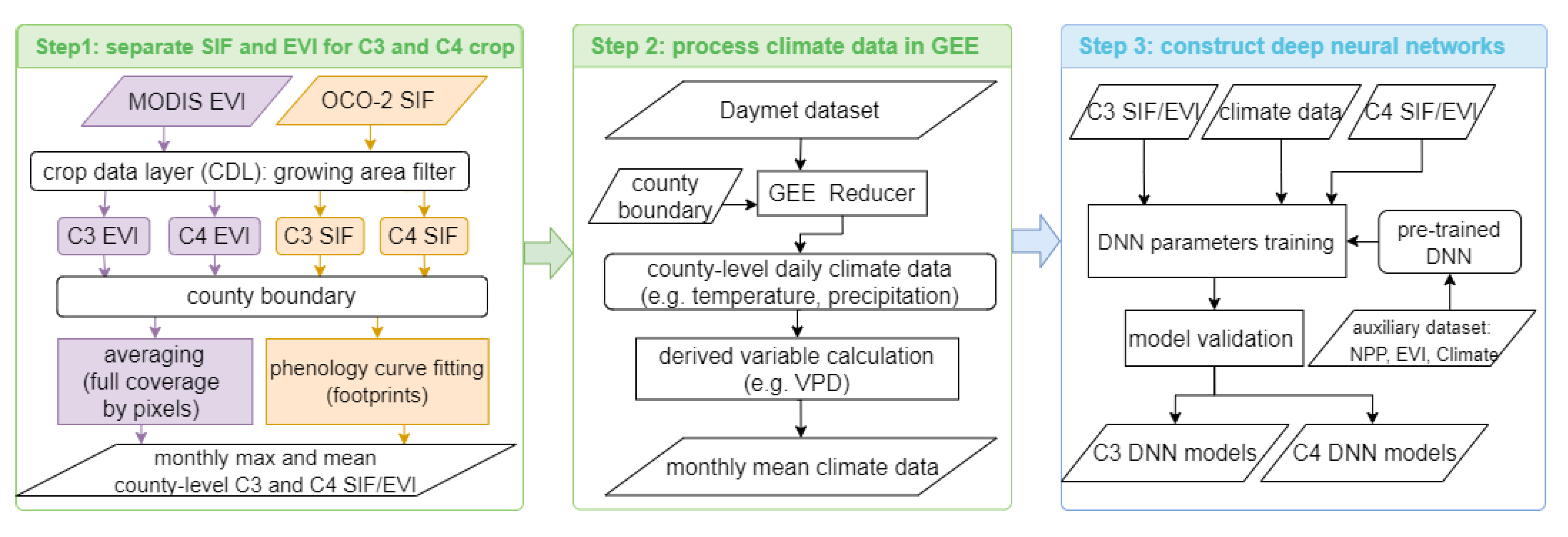
We used the United States Department of Agriculture (USDA) National Agricultural Statistics Service (NASS) Crop Data Layer (CDL) data to identify areas of corn and soybeans from 2015 to 2017. The CDL data are annual land cover classification products with a spatial resolution of 30 m. The data of county-level soybean and maize yields were retrieved from the USDA Quick Statistic Database.

The CDL data in each year from 2015 to 2017 were employed to determine whether a MODIS EVI pixel and an OCO-2 footprint belong to the soybean or maize category. The area ratios of soybean and maize within all pixels and footprints were calculated. Only pixels and footprints with the area ratio of soybean or maize above 60% were selected for further analysis. A threshold of 60% was used for balancing the tradeoff between the relative purity of the pixels and the availability of the data. A similar value was employed in a previous study to identify vegetation types covered by OCO-2 footprints [62]. For a county, the three-year mean EVI of soybean and maize was calculated for each month in the growing season (from May to September) according to values of selected individual pixels, i.e.,

$$\overline{EV{I}_m}=\frac{1}{3}{\displaystyle \sum _{y=1}^3}(\frac{1}{N_y}{\displaystyle \sum _{p=1}^{N_y}}EV{I}_{y,m,p})$$

(1)

where $\overline{EV{I}_m}$ is the three-mean of EVI in month m; EVI_y,m,p is the EVI value of the p^th pixel in month m of the y^th year; N_y is the number of pixels belong to corn or soybean in the y^th year.

OCO-2 SIF data was spatially discrete and there are gaps between nearby swaths (Figure 1). Within a county, SIF might be observed on different adjacent days for a given period. The variation of SIF caused by the difference in observing dates must be taken into account. Therefore, the county-level three-year SIF means of soybean and maize were generated in the following way. All SIF observations of soybean and maize in all three years within each county were lumped together to fit phenology curves of individual crop types (Section 2.3.1) since observations of SIF in one year were very limited for a county. Two respective phenology curves of soybean and maize were constructed for each county. With the fitted curves, daily SIF during the growing season was simulated for each county. With simulated daily SIF, monthly means and maxima of SIF were calculated.

2.3. Method

2.3.1. SIF Phenology Fitting

A double-sigmoidal function was used to fit the seasonal cycle SIF representing photosynthetic status signals for each county [73]. It has the advantage of retrieving vegetation phenology with noisy data [74,75], such as OCO-2 SIF. This equation is as follows:

$$y\left(x\right)=a_1+\frac{a_2}{1+\exp (-d_1\left(x-b_1\right))}-\frac{a_3}{1+\exp (-d_2\left(x-b_2\right))}$$

(2)

where y represents the SIF value, x is a given day of the year (DOY); a₁ represents the SIF value in the winter; a₂ and a₃ represent values at the spring and autumn plateau, respectively; b₁ and b₂ are the DOY mid-points of transitions for spring greenup and autumn browndown, respectively; and d₁ and d₂ are the corresponding slope coefficients of these transitions.

Parameters (a₁–a₃, b₁, b₂, d₁, d₂) on the right of Equation (2) were fitted using three-year mean SIF in different months by a genetic algorithm [73]. Only counties with seasonal curves of SIF well fitted (R² > 0.8) were used for further analysis. Finally, there were a total of 218 and 201 counties with SIF data available for maize and soybean, respectively. For all of these available counties, three-year means of EVI and climate data were accordingly calculated for all individual months from May to September.

2.3.2. Model Construction and Validation

The machine learning method adopted here is DNN, one of the typical deep learning algorithms. The DNN has the advantage of learning complex, non-linear relationships and extracting intricate information effectively through the process of transforming raw inputs (satellite and climate data here) gradually towards a higher level of information [34,76,77], e.g., crop yields in this case. DNN used in this study is a feed-forward neural network (NN) with architectures of multiple fully connected layers. Layers in NN can be categorized into the input, hidden, and output layers, and each layer is composed of a certain number of neurons. The number of input neurons is equal to the number of inputs (three-year means of monthly EVI, SIF, and climate variables).

DNN has a large number of hyper-parameters and weights, which require sufficient training data to prevent overfitting and to achieve good model performance. However, due to the low data availability of OCO-2 SIF, it is difficult to collect adequate training, validation, and testing to optimize hyperparameters while testing the trained DNN unbiasedly. Transfer learning (TL) between similar tasks, therefore, becomes desirable for overcoming this problem. Theoretically, this technique enables the leveraging of data and knowledge from a source domain to facilitate modeling in a related target domain, and thus alleviates difficulties and efforts of data collecting and model building [78]. Additionally, the TL technique, unlike the traditional machine learning methods, does not require the training and targeted data in the same feature space and have the same distribution [79]. Based on the rationale of TL, we selected NPP, EVI, and climate data as the source dataset considering the close link between crop NPP and yield. We then built DNNs by transferring the knowledge of employing EVI and climate data to predict NPP to our targeted task of using a similar dataset to predict crop yields. A detailed description of the transferring process is as follows: before the construction and validation of DNN models, all variables were standardized into features with zero mean and unit variance, including yields and NPP of maize and soybean (dependent variables), and three-year means of monthly SIF, EVI, and climate data from May to September (independent variables). Then, we pre-trained the structure of DNN using county-level mean annual NPP and monthly mean EVI from May to September in years 2013 and 2014 to determine hyper-parameters, such as the number of hidden layers and neurons in each layer (Appendix A). The trained network structure is shown in Figure S3. With the DNN architecture obtained above, the weights in each layer were optimized with the training subsets of the targeted dataset (the three-year-mean crop yield, SIF, EVI, and climate data) for corn and soybean, respectively.

The repeated five-fold cross-validation (CV) technique [80] was used to separate the targeted dataset into training and testing groups. In each iteration, the targeted dataset was first shuffled randomly and then split into five equal-sized subsets, of which four subsets of data were used for training the model and the remaining one subset was used for testing the model. The training and testing processes were repeated until all five subsets of data had been used for model tests. All estimated corn and soybean yields in all five test processes were combined to produce a complete validation dataset for this iteration. This whole process of five-fold CV was then iterated 100 times. The validation scores of the 100 runs were averaged for further analysis.

The performance of models was evaluated with statistical metrics, including R², mean absolute error (MAE), mean absolute percentage error (MAPE), and percentage error (PE):

$$\mathrm{MAE}=\frac{1}{n}{\sum }_{i=1}^n\left|Y_{m,i}-Y_{e,i}\right|$$

(3)

$$\mathrm{MAPE}=\frac{MAE}{\frac{1}{n}{\sum }_{i=1}^n{Y}_{m,i}}$$

(4)

$$P{E}_i=\frac{Y_{m,i}-Y_{e,i}}{Y_{m,i}}\times 100$$

(5)

where $Y_e$ is the crop yield estimated by the model, $Y_m$ is the three-year-mean crop yield calculated based on measured data from USDA, $i$ indicates a given county, and n is the number of available records.

2.3.3. Importance Determination of Different Variables

The feature importance (FI) analysis was employed to identify the importance of different variables in crop yield prediction. The ‘feature’ here refers to model predictors, including SIF, EVI, and climate variables. The FI technique randomly permutates the values of one feature while keeping the values of remaining features unchanged and then evaluates the relative importance of the aimed feature by measuring the reduction of model performance [81]. The rationale behind this algorithm is that by shuffling the feature values randomly, meaningful information of the feature is replaced with random noise. As a result, the association between feature and response variables is broken, leading to the decrease of the variance explained by the model (R²) [82,83]. In the current study, we calculate FI scores by averaging the results from the 100 repeated experiments, and the FI score for a feature is defined as follows:

$$F{I}_{feature}=R_{original}^2-\frac{1}{M}{\sum }_{i=1}^M{R}_{shulffled}^2$$

(6)

where $R_{original}^2$ is the R² of the original model without permutation and $R_{shulffled}^2$ is the value of the model after permutating the feature variable; M is the number of times the feature is shuffled, which aims to increase the robustness of the method [81].

3. Results

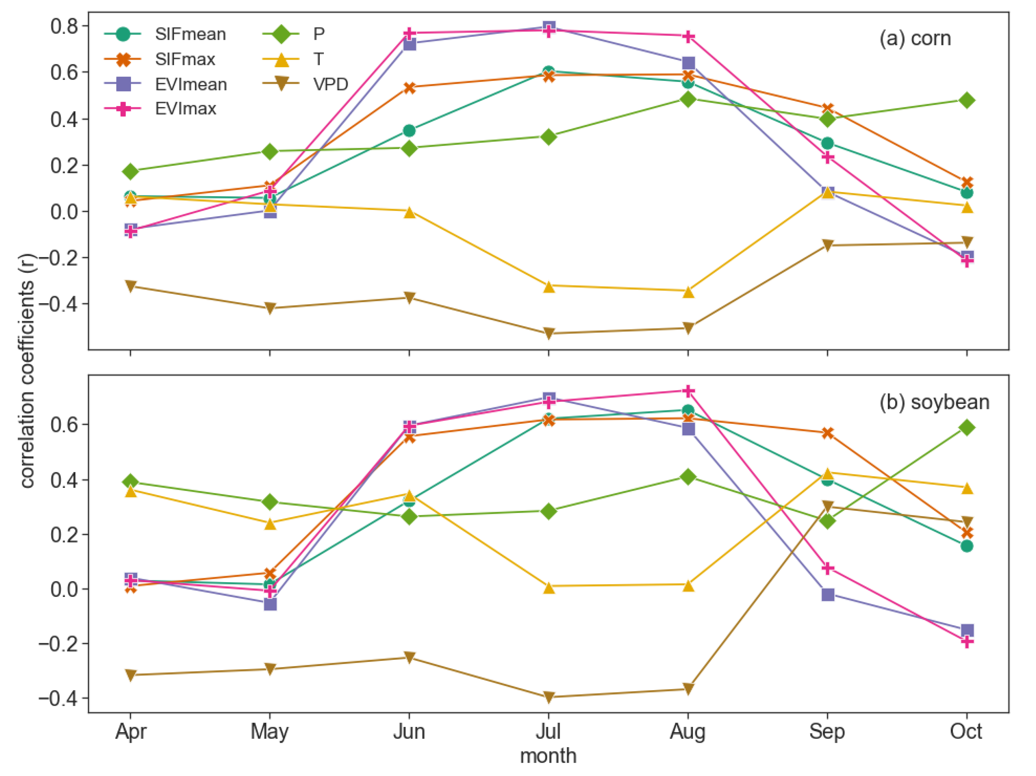
3.1. Relationships Between Crop Yields and Different Variables

The relationships of crop yields with monthly SIF, EVI, and climate variables were quantified using the Pearson product–moment correlation coefficients (r) (Figure 3). Monthly VPD generally had negative correlations with both corn and soybean yields, especially in the peak growing season (June, July, and August) (p < 0.05) (Table S5). Precipitation in all months was positively correlated with both corn and soybean yields. Correlations of monthly means and maxima of SIF and EVI with corn and soybean yields sharply increased from May to June and then decreased from August to October. In September and October, SIF showed stronger positive correlations with the yields than EVI. In most of the months, both monthly maxima of SIF and EVI performed better in indicating the yields than the corresponding monthly means. Therefore, monthly maxima of SIF and EVI were used in further analysis.

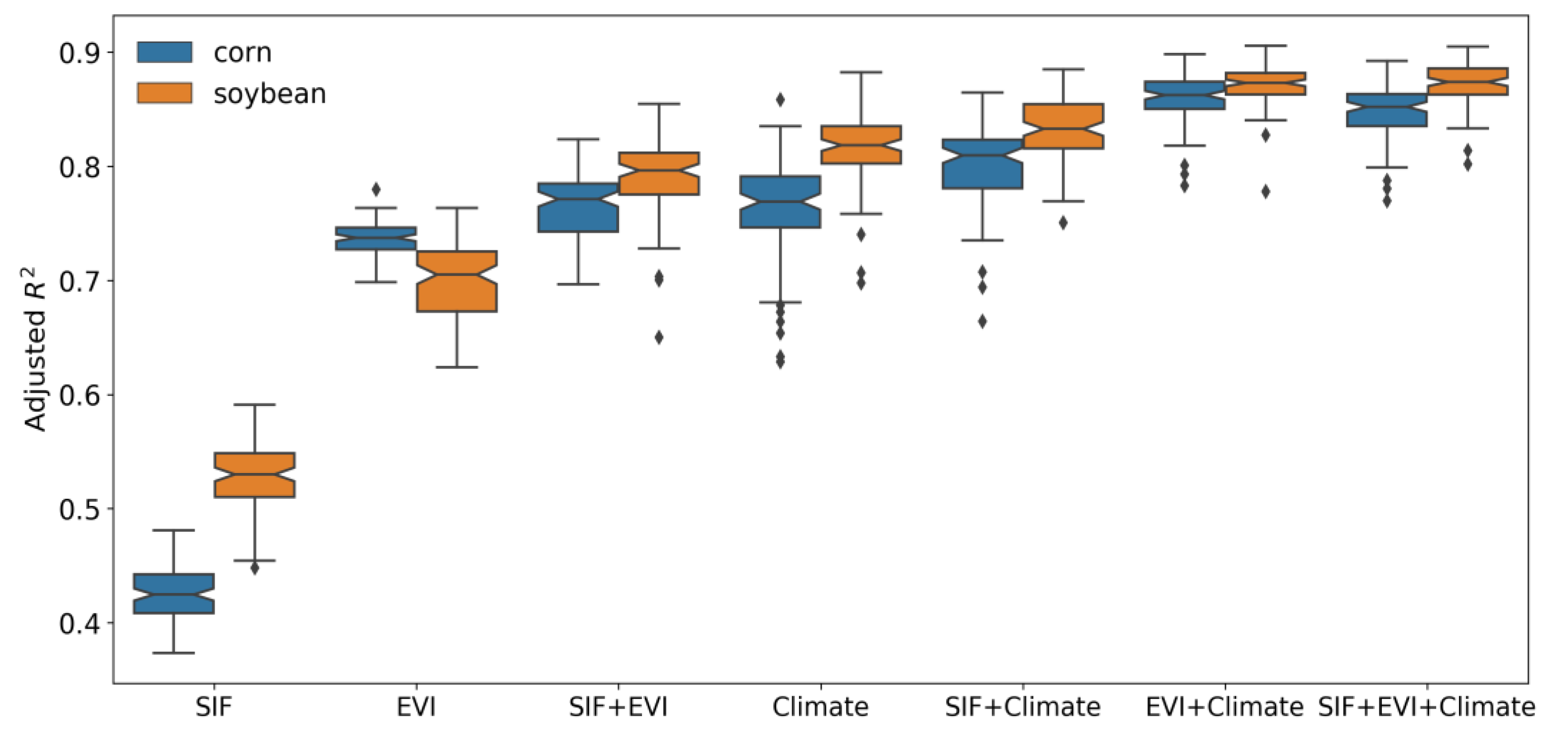
3.2. Performances of DNNs for Corn and Soybean Yield Prediction

County-level yields of corn and soybean, monthly means of climate (T, P, and VPD) and maxima of EVI and SIF from May to September were used to train DNN models.

Table 1. Averaged performances of DNNs models for predicting county-level corn and soybean yields in the Midwestern 12 states. ^a

Models	N	Corn			Soybean
		R2	MAE	MAPE (%)	R2	MAE	MAPE (%)
SIF	5	0.43	16.50	8.99	0.53	4.73	8.90
EVI	5	0.74	10.26	5.59	0.70	3.51	6.79
SIF + EVI	10	0.76	9.62	5.24	0.79	3.05	5.89
Climate	15	0.76	9.76	5.34	0.82	2.87	5.55
SIF + Climate	20	0.80	8.98	4.90	0.83	2.68	5.18
EVI + Climate	20	0.86	7.27	3.97	0.87	2.36	4.56
SIF + EVI + Climate	25	0.85	7.49	4.08	0.87	2.30	4.45

^a The R² values are the adjusted R². The unit of MAE is bushels per acre. N is the number of predictors in each model.

shows the performances of DNN models with different combinations of inputs. Models with inputs of SIF, EVI, SIF plus EVI, and Climate have moderate to high coefficients of determination, indicating the usefulness of satellite and climate information in predicting corn and soybean yields. Among models only with EVI, SIF, and climate as inputs, the models with climate predictors performed the best, explaining 76% and 82% variations of county-level corn and soybean yields, respectively. Models only with monthly maximum SIF as inputs performed the poorest. The integration of SIF and EVI could improve the performance of yield estimating models that only used either SIF or EVI data as predictors. In addition, the combination of satellite and climate data significantly improved model performances. Specifically, models with both EVI and climate as inputs outperformed the climate-based models, increasing R² from 0.76 to 0.86 for corn and from 0.82 to 0.87 for soybean. The combination of climate information with SIF also improved the estimates of the yields, with R² increased from 0.76 to 0.80 for corn and from 0.82 to 0.83 for soybean. These results suggest that OCO-2 SIF could make some contributions to the yield estimate, but less than MODIS EVI. The models with all SIF, EVI, and climate variables as inputs performed similar to the models with EVI and climate as inputs, implying that OCO-2 SIF provided less useful information for capturing the spatial variations of corn and soybean yields in the study area than EVI.

The analysis of variance (ANOVA) and the Tukey Honest Significant Difference (HSD) tests [84] were conducted to investigate whether the differences among model performances in the 100 repeated experiments are significant (Tables S2 and S3). The ANOVA tests for both corn and soybean showed significant differences among performances of different models (p < 0.001). Additionally, the Tukey HSD tests demonstrated that most of the performance differences between paired models were significant, except for the differences between ‘EVI + Climate’ and ‘SIF + EVI + Climate’ models for both corn and soybean, and between ‘Climate’ and ‘SIF + EVI’ for corn. These results further confirmed that the addition of SIF data into the ‘EVI + Climate’ models did not improve the estimates of both corn and soybean yields. However, there are significant differences between the ‘EVI’ and the ‘SIF + EVI’ models, and between the ‘Climate’ and the ‘SIF + Climate’ models. This indicated that the inclusion of SIF could improve the ‘Climate’ model and ‘EVI’ model for estimating yields of corn and soybean.

The performances and stability of DNNs were compared by summarizing the repeated CV results. As shown in Figure 4, the ‘Climate’ model had lower minimum and first quantile values of R² than those of the ‘SIF + Climate’ and ‘EVI + Climate’ models for both corn and soybean. This means that, even for the worst cases, the models with both satellite and climate predictors outperformed the models with only climate data as inputs. A similar finding was also observed between the ‘SIF + EVI’ and ‘EVI’ models for soybean, and the former performed better than the latter under the worst and other conditions. The interquartile range (IQR) and overall range of R² of ‘EVI + Climate’ and ‘SIF + EVI + Climate’ models were noticeably smaller than those of the ‘Climate’ models for both corn and soybean (Table S4), indicating that the overall performance of ‘EVI + Climate’ and ‘SIF + EVI + Climate’ models varied at a lower degree among different experiments than the ‘Climate’ model. This result demonstrated that the addition of EVI and SIF data into the climate-based models enhanced the stability of DNN performances and the reliability of yield estimates under different conditions.

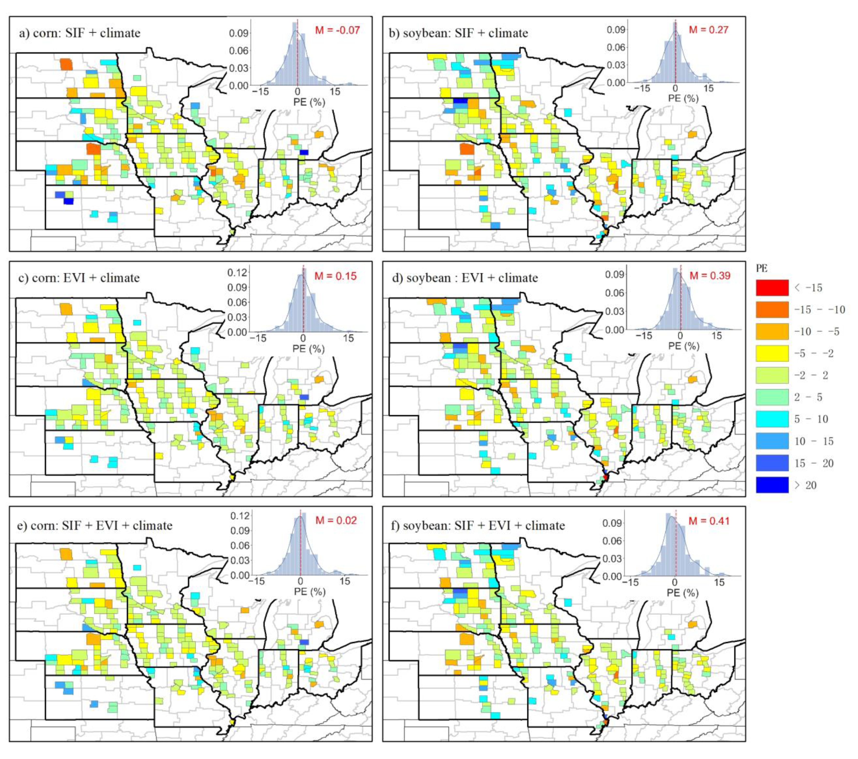
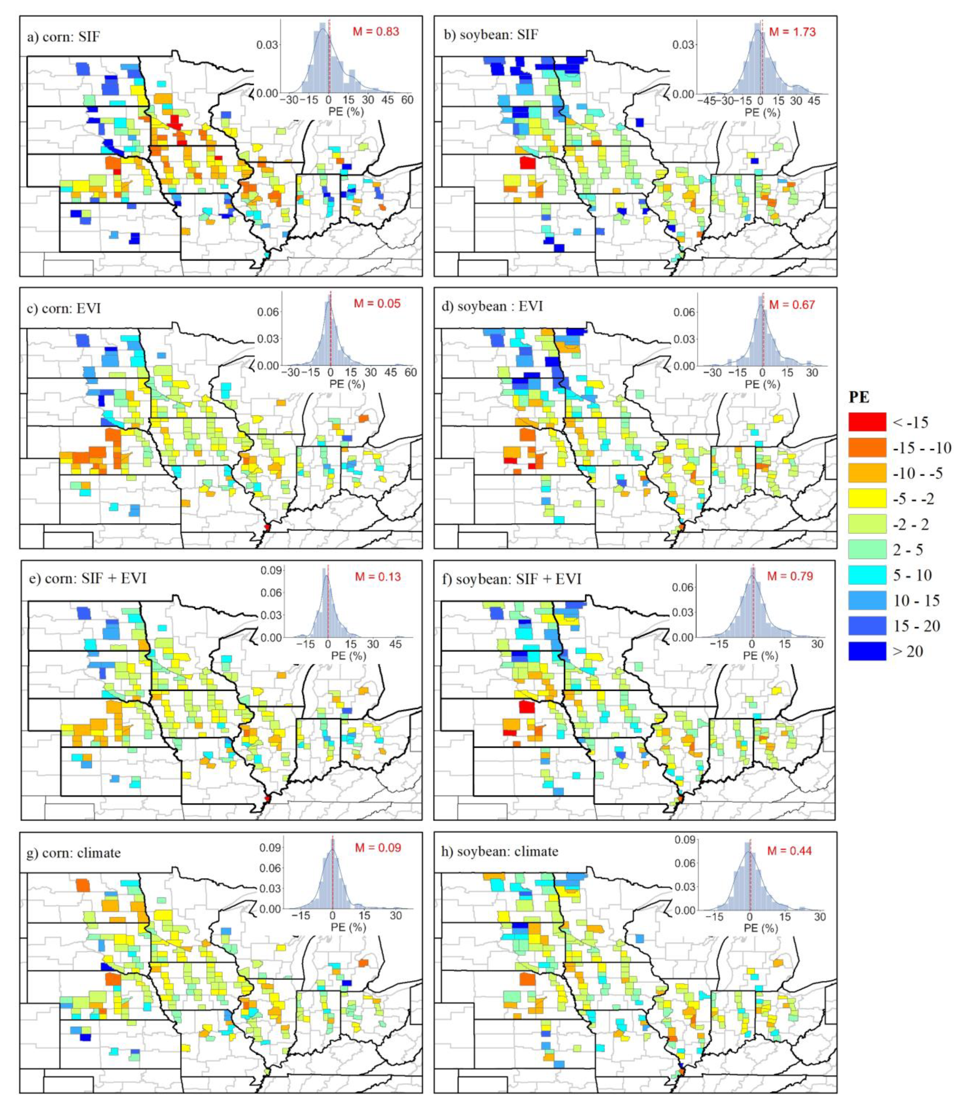
3.3. Spatial Differences in Performances of the DNN Models

Figure 5 and Figure 6 show the spatial distribution of PE for different models. The spatial patterns of PE for both corn and soybean were similar among the ‘EVI + Climate,’ ‘SIF + Climate,’ and ‘SIF + EVI + Climate’ models. In particular, those models performed similarly well in the central part of the Corn Belt (e.g., Iowa). The magnitudes of PE were mostly smaller than ±2%. In contrast, PE was higher in the northern part of the Midwest states (i.e., North Dakota, northern South Dakota, and northwestern Minnesota), which indicates that models tended to underestimate yields of soybean in these regions (Figure 5b,d,f). The underestimation of corn and soybean yields by ‘EVI’, ‘SIF’, and ‘SIF + EVI’ models were also significant in the northwestern part of the study area (Figure 6b,d,f). In contrast, the PE values of models with only climate variables as inputs showed less spatial variability (Figure 6h).

For corn, the PE values of models based only on SIF, EVI, and climate inputs ranged from −20.25% to 47.03%, from −26.11% to 46.09%, and from 15.68% to 30.85% (

Table 2. Summary of the percentage error (PE) of county-level yields estimated by different models in the 12 Midwest states. Values fall into columns of 15%, 50%, 85% are the PE at the 15th, 50th (or median), and 85th percentile.

Corn	Min	15%	50%	85%	Max	Mean	Std a
SIF	−20.25	−10.03	−1.87	13.91	47.03	0.83	11.97
EVI	−26.11	−6.39	−0.64	6.32	46.09	0.05	7.84
SIF + EVI	−20.20	−5.69	−0.50	5.70	47.83	0.13	6.89
Climate	−15.68	−4.52	−0.11	4.24	30.85	0.09	5.78
SIF + Climate	−12.46	−4.72	−0.65	3.78	21.90	−0.07	5.12
EVI + Climate	−12.28	−3.48	−0.17	3.75	15.93	0.15	3.97
SIF + EVI + Climate	−11.44	−3.55	−0.08	3.39	17.83	0.02	4.23
Soybean	Min	15%	50%	85%	Max	Mean	Std a
SIF	−36.86	−9.42	0.03	12.67	40.62	1.73	12.37
EVI	−28.96	−6.18	0.07	7.14	29.35	0.67	8.43
SIF + EVI	−17.06	−5.23	0.27	6.29	25.18	0.79	6.49
Climate	−13.80	−5.35	−0.15	5.54	23.48	0.44	5.94
SIF + Climate	−14.53	−4.80	0.12	5.11	21.94	0.27	5.44
EVI + Climate	−15.64	−4.37	−0.16	4.65	18.68	0.39	4.89
SIF + EVI + Climate	−11.30	−3.63	−0.25	4.27	16.74	0.41	4.57

^a Std = standard deviation.

). It was also found that the combination of remote sensing and climate data made the range of PE much smaller, i.e., −12.46% to 21.90 for the model based on SIF and climate, −12.28% to 15.93% for the model based on EVI and climate, and −11.44% to 17.83 for the model with SIF, EVI, and climate data as inputs. As for soybean, the PE ranges by individual models are similar to those of corn. In addition, the DNN models performed well at the county level for both crop types. For above 70% of counties, PE values of ‘EVI + Climate’ and ‘SIF + EVI + Climate’ models ranged from −3.48% to 3.75% and from −3.55% to 3.39% for corn. The corresponding values were from −4.37% to 4.65% and from −3.63% to 4.27% for soybean (Table 2).

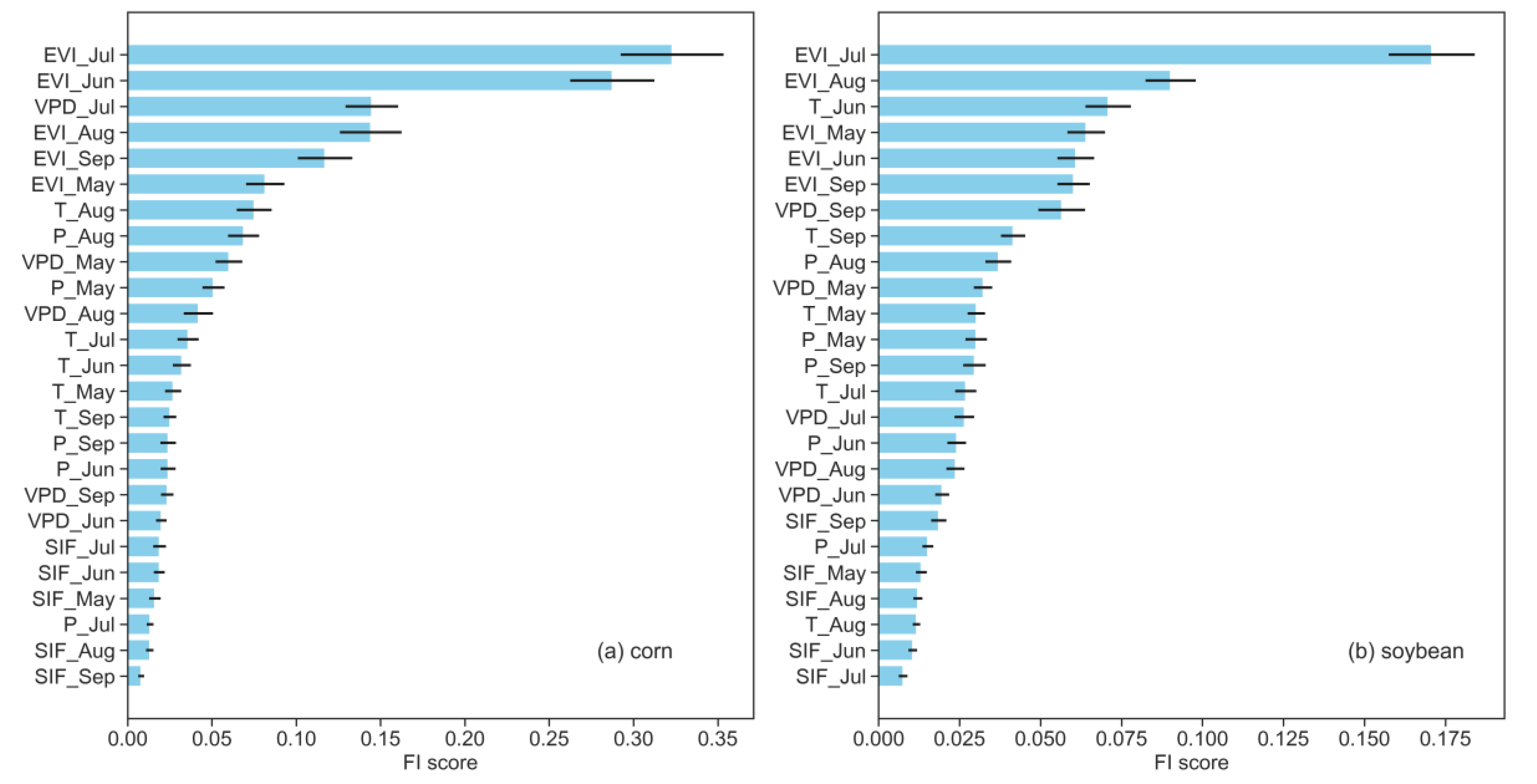
3.4. Importance of Different Variables

The feature importance (FI) scores of predictors in the ‘EVI + SIF + Climate’ models were calculated for examining the importance of individual predictors in estimating corn and soybean yields. The ‘EVI + SIF + Climate’ models were used because they included the most comprehensive inputs relative to other models using only satellite or climate predictors. Figure 7 shows the importance of the variables in predicting corn and soybean yields, with a higher FI value indicating a greater contribution to the model performances. It should also be noted that the FI analysis is model-specific because different variables might have dissimilar functions in different DNNs, and the FI results for other models were presented in Figures S4–S6.

In the ‘EVI + SIF + Climate’ model, both satellite and climate predictors in the peak growing months (from June to August), which is corresponding with the grain filling and reproductive periods in the Midwestern U.S. [85], were essential in estimating crop yields. Specifically, EVI in July was the most important variable determining yields of both corn and soybean. In this month, corn and soybean here started the reproductive stage [45,86], and EVI effectively captures the growing status of the crop. EVI in August is the second important factor for predicting soybean yield and the third important remote sensing factor for predicting corn yield in the Midwest states, which was also confirmed by a previous study [46]. They declared that the inclusion of EVI in August noticeably reduced the uncertainty of yield prediction. As for climate variables, VPD in July and temperature in June acted as the important determinants for yields of corn and soybean, respectively. VPD has a strong impact on the stomatal conductance of crops, which affects carbon assimilation [7,87,88]. As shown in Figure 3, VPD in July had a significant negative correlation with the corn yield. Temperature determines VPD and influences photosynthetic activities, and thus constrains biomass production and influences crop yield [89,90,91]. In the study region, the temperature in June played an important role in determining the yield of soybean, just following EVI in July and August (Figure 3 and Figure 7). SIF was generally less important for estimating corn and soybean yields in comparison with EVI and climate variables. The information carried by SIF into the model might be overshadowed by EVI. As shown in Table 1, ‘EVI + SIF + Climate’ and ‘EVI + Climate’ models performed very similarly.

4. Discussion

SIF is tightly linked with vegetation photosynthesis at various temporal scales. Theoretically, SIF has the potential to be an effective predictor of crop yields, because it is associated with electron transport in light reaction of photosynthesis, and therefore, closely related to GPP of plants [48,49,64]. However, the spatial resolution of most available satellite SIF is relatively low (40 km × 80 km for GOME-2 SIF and 30 km × 60 for SCIAMACHY SIF), and it is difficult to use such low-resolution satellite SIF to estimate crop yields at small scales, such as the county-level. The spatial resolution of OCO-2 SIF is much higher than those of GOME-2 and SCIAMACHY. However, the swath width of OCO-2 is only 10.3 km. There are gaps around 100 km between two adjacent swaths [92]. The spatial and temporal discontinuities of OCO-2 SIF hinder the application of these data in estimating crop yields at regional scales.

In this study, three years of OCO-2 SIF data in different months were used to fit the phonology curves of corn and soybean for individual counties. With the fitted curves, monthly SIF means and maxima were estimated for corn and soybean in different counties. These monthly SIF values in the peak growing season were significantly positively correlated with three-year mean county-level corn and soybean yields (Figure 3), confirming that SIF is an effective indicator of crop yields owing to its direct linkage with photosynthesis. However, compared to EVI, our processed SIF had relatively weaker correlations with corn and soybean yields (Figure 3) and poor ability to capture the spatial variations of yields (Table 1). This is due to the fact that the county-level EVI used here was calculated from spatially and temporally continuous direct observations by the satellite, while the SIF values used were estimated from the phenology curves which were fitted from limited direct observations in three years. The numbers of SIF observations were uneven for a county, and locations of footprints might differ in different years. The discrepancy between estimated and real county-level mean SIF would definitely weaken the effectiveness of OCO-2 SIF data in predicting crop yields. Therefore, the development of spatially and temporally continuous high-resolution SIF datasets is required for improving estimates of crop yields.

In the study area, climate-based DNN models overall performed better than remote sensing-based DNN models in capturing spatial variations of county-level corn and soybean yields, possibly due to the strong controls of VPD and precipitation on yields (Figure 3). In addition, the departures of yields estimated by climate-based DNN models from census data showed less spatial variations relative to those form SIF and EVI-based DNN models (Figure 6). These results indicated that climate information played a more important role in controlling the spatial variations of corn and soybean yields in this region. EVI was an effective indicator of crop biomass, which is tightly linked with final yields. Therefore, the performance of EVI-based DNN models was close to that of climate-based DNN models (Table 2 and Figure 4). However, similar to SIF-based models, EVI-based models performed poorer than climate-based models in counties with low area fractions of corn and soybean (Figure 6 and Figure S2), indicating that there were impacts of land cover heterogeneity on crop estimates by remote sensing data.

The combination of different sources of data might improve crop yield estimation (Table 1). Although, when compared with other model variables, our estimated county-level mean SIF showed relatively poor ability to capture spatial variations of corn and soybean yields, it could act as effective supplement information of EVI and climate for better estimating crop yields. DNN models inputting both SIF and EVI data performed very close to climate-based DNN models. Additionally, DNN models integrating EVI and climate data outperformed either EVI or climate-based models (Figure 4 and Figure 5, and Figure 6; Table 1 and Table 2). However, the addition of data from the same source could not constrain yield estimate. From the statistical point of view, DNN models with SIF, EVI, and climate data as inputs performed even slightly poorer than models with EVI and climate (Table 1). The spatial patterns of discrepancies between yields estimated by two models and census data were also similar (Figure 5).

Nevertheless, satellite SIF data is useful for estimating crop yields even if current SIF products have some limitations. The launching of satellite with finer resolution and broader spatial coverage than OCO-2, such as FLEX [93] and GeoCARB [94], would pave the way for further testing to what degree SIF might contribute to crop yields estimation from space. Currently, one possible solution for estimating crop yield using SIF data is to downscale satellite SIF data. For example, several studies have proposed methods to produce spatially continuous high spatial resolution SIF datasets using OCO-2 SIF measurements [95,96,97]. It is worthy of investigating the applicability of such downscaled SIF in estimating crop yields.

Furthermore, it should be noted that when predicting crop yield empirically, especially when employing sophisticated machine learning techniques such as DNN, it would be beneficial to collect more training data. In addition, information other than EVI or SIF could also be useful in predicting corn and soybean yield and boosting the model performance as additional predictors. For example, vegetation optical depth (VOD) derived from the satellite passive microwave bands could indicate canopy biomass and water content condition of the plants [35,98,99]; evaporative stress index (ESI) retrieved from satellite thermal bands and leaf area index is desirable for assessing the crop moisture status as an indicator of agricultural drought [100,101]. Furthermore, it is expected that with more data and more comprehensive predictors, the model could extract information more effectively and better discover non-linear relationships between dependent and independent variables. Therefore, our future work would further test the usefulness of SIF signals in crop yield predicting when more data are available. We would also employ multiple sources of data for crop yield predicting via the DNN technique, aiming to build a high-performance crop yield forecasting system at the regional level.

5. Conclusions

In this study, we proposed a method to use the OCO-2 SIF product to predict yields of corn and soybean in the U.S. Corn Belt. The ability of OCO-2 SIF products to estimate county-level crop yields in the study area was compared with those of MODIS EVI and conventional climate data. The following conclusions could be drawn from this study.

(1) Monthly mean and maximum SIF during the peak growing season showed similar significant correlations with corn and soybean yields to MODIS EVI. The DNNs with SIF as predictors were able to capture spatial variations of corn and soybean yields but performed much poorer than those based on MODIS EVI and climate variables. The performance of SIF and MODIS EVI-based DNNs varied with the areal dominance of crops. In areas with low areal fraction of crops, the SIF and EVI-based DNNs tended to underestimate corn and soybean yields noticeably. The performance of DNNs with climate variables as predictors exhibited less spatial variability.

(2) The combination of remote sensing and climate data improved the estimation of crop yields. Our processed county-level SIF data could provide useful supplementary information to MODIS EVI and climatic variables in estimating crop yields. DNNs of EVI and climatic variables in conjunction with SIF obliviously outperformed DNNs with only EVI or climatic variables as predictors. The integration of MODIS EVI and climatic variables was able to improve the estimating accuracy of crop yields significantly. Further addition of SIF into models with MODIS EVI and climatic variables only marginally enhanced crop yields prediction.

(3) Feature importance analysis indicated that MODIS EVI and climate predictors (e.g., VPD and temperature) during the peak growing season (from June to August) played critical roles in predicting yields of corn and soybean in the Midwestern 12 states in the U.S. for the DNNs with all SIF, EVI, and climatic variables as predictors. By contrast, the importance of SIF was much smaller than MODIS EVI and climatic variables in those DNNs.

References

1. Horie, T.; Yajima, M.; Nakagawa, H. Yield Forecasting. Agric. Syst. 1992, 40, 211–236. [Google Scholar] [CrossRef]
2. Basso, B.; Cammarano, D.; Carfagna, E. Review of crop yield forecasting methods and early warning systems. In Proceedings of the First Meeting of the Scientific Advisory Committee of the Global Strategy to Improve Agricultural and Rural Statistics, FAO Headquarters, Rome, Italy, 18–19 July 2013; pp. 18–19. [Google Scholar]
3. Adjemian, M.K.; Smith, A. Using USDA Forecasts to Estimate the Price Flexibility of Demand for Agricultural Commodities. Am. J. Agric. Econ. 2012, 94, 978–995. [Google Scholar] [CrossRef]
4. Hoffman, L.A.; Etienne, X.L.; Irwin, S.H.; Colino, E.V.; Toasa, J.I. Forecast performance of WASDE price projections for US corn. Agric. Econ. 2015, 46, 157–171. [Google Scholar] [CrossRef]
5. Mkhabela, M.S.; Mkhabela, M.S.; Mashinini, N.N. Early maize yield forecasting in the four agro-ecological regions of Swaziland using NDVI data derived from NOAA’s-AVHRR. Agric. For. Meteorol. 2005, 129, 1–9. [Google Scholar] [CrossRef]
6. Challinor, A. AGRICULTURE Forecasting food. Nat. Clim. Chang. 2011, 1, 103–104. [Google Scholar] [CrossRef]
7. Lobell, D.B.; Hammer, G.L.; McLean, G.; Messina, C.; Roberts, M.J.; Schlenker, W. The critical role of extreme heat for maize production in the United States. Nat. Clim. Chang. 2013, 3, 497–501. [Google Scholar] [CrossRef]
8. Iizumi, T.; Luo, J.J.; Challinor, A.J.; Sakurai, G.; Yokozawa, M.; Sakuma, H.; Brown, M.E.; Yamagata, T. Impacts of El Nino Southern Oscillation on the global yields of major crops. Nat. Commun. 2014, 5, 3712. [Google Scholar] [CrossRef] [Green Version]
9. Lesk, C.; Rowhani, P.; Ramankutty, N. Influence of extreme weather disasters on global crop production. Nature 2016, 529, 84–87. [Google Scholar] [CrossRef]
10. Muller, C.; Elliott, J.; Chryssanthacopoulos, J.; Arneth, A.; Balkovic, J.; Ciais, P.; Deryng, D.; Folberth, C.; Glotter, M.; Hoek, S.; et al. Global gridded crop model evaluation: Benchmarking, skills, deficiencies and implications. Geosci. Model Dev. 2017, 10, 1403–1422. [Google Scholar] [CrossRef] [Green Version]
11. Peng, B.; Guan, K.Y.; Chen, M.; Lawrence, D.M.; Pokhrel, Y.; Suyker, A.; Arkebauer, T.; Lu, Y.Q. Improving maize growth processes in the community land model: Implementation and evaluation. Agric. For. Meteorol. 2018, 250, 64–89. [Google Scholar] [CrossRef]
12. Bassu, S.; Brisson, N.; Durand, J.L.; Boote, K.; Lizaso, J.; Jones, J.W.; Rosenzweig, C.; Ruane, A.C.; Adam, M.; Baron, C. How do various maize crop models vary in their responses to climate change factors? Glob. Chang. Boil. 2014, 20, 2301–2320. [Google Scholar] [CrossRef] [PubMed]
13. Van der Werf, W.; Keesman, K.; Burgess, P.; Graves, A.; Pilbeam, D.; Incoll, L.; Metselaar, K.; Mayus, M.; Stappers, R.; van Keulen, H. Yield-SAFE: A parameter-sparse, process-based dynamic model for predicting resource capture, growth, and production in agroforestry systems. Ecol. Eng. 2007, 29, 419–433. [Google Scholar] [CrossRef] [Green Version]
14. Iizumi, T.; Yokozawa, M.; Nishimori, M. Parameter estimation and uncertainty analysis of a large-scale crop model for paddy rice: Application of a Bayesian approach. Agric. For. Meteorol. 2009, 149, 333–348. [Google Scholar] [CrossRef]
15. Lobell, D.B.; Burke, M.B. On the use of statistical models to predict crop yield responses to climate change. Agric. For. Meteorol. 2010, 150, 1443–1452. [Google Scholar] [CrossRef]
16. Shi, W.J.; Tao, F.L.; Zhang, Z. A review on statistical models for identifying climate contributions to crop yields. J. Geogr. Sci. 2013, 23, 567–576. [Google Scholar] [CrossRef]
17. Li, Y.; Guan, K.Y.; Yu, A.; Peng, B.; Zhao, L.; Li, B.; Peng, J. Toward building a transparent statistical model for improving crop yield prediction: Modeling rainfed corn in the U.S. Field Crop. Res. 2019, 234, 55–65. [Google Scholar] [CrossRef]
18. Mirschel, W.; Wieland, R.; Wenkel, K.-O.; Nendel, C.; Guddat, C. YIELDSTAT–a spatial yield model for agricultural crops. Eur. J. Agron. 2014, 52, 33–46. [Google Scholar] [CrossRef]
19. Kern, A.; Barcza, Z.; Marjanovic, H.; Arendas, T.; Fodor, N.; Bonis, P.; Bognar, P.; Lichtenberger, J. Statistical modelling of crop yield in Central Europe using climate data and remote sensing vegetation indices. Agric. For. Meteorol. 2018, 260, 300–320. [Google Scholar] [CrossRef]
20. Gornott, C.; Wechsung, F. Statistical regression models for assessing climate impacts on crop yields: A validation study for winter wheat and silage maize in Germany. Agric. For. Meteorol. 2016, 217, 89–100. [Google Scholar] [CrossRef]
21. Lobell, D.B. Changes in diurnal temperature range and national cereal yields. Agric. For. Meteorol. 2007, 145, 229–238. [Google Scholar] [CrossRef]
22. Johnson, M.D.; Hsieh, W.W.; Cannon, A.J.; Davidson, A.; Bedard, F. Crop yield forecasting on the Canadian Prairies by remotely sensed vegetation indices and machine learning methods. Agric. For. Meteorol. 2016, 218, 74–84. [Google Scholar] [CrossRef]
23. Pantazi, X.E.; Moshou, D.; Alexandridis, T.; Whetton, R.L.; Mouazen, A.M. Wheat yield prediction using machine learning and advanced sensing techniques. Comput. Electron. Agric. 2016, 121, 57–65. [Google Scholar] [CrossRef]
24. Cai, Y.P.; Guan, K.Y.; Lobell, D.; Potgieter, A.B.; Wang, S.W.; Peng, J.; Xu, T.F.; Asseng, S.; Zhang, Y.G.; You, L.Z.; et al. Integrating satellite and climate data to predict wheat yield in Australia using machine learning approaches. Agric. For. Meteorol. 2019, 274, 144–159. [Google Scholar] [CrossRef]
25. You, J.; Li, X.; Low, M.; Lobell, D.; Ermon, S. Deep gaussian process for crop yield prediction based on remote sensing data. In Proceedings of the Thirty-First AAAI Conference on Artificial Intelligence, San Francisco, CA, USA, 4–9 February 2017. [Google Scholar]
26. Bose, P.; Kasabov, N.K.; Bruzzone, L.; Hartono, R.N. Spiking Neural Networks for Crop Yield Estimation Based on Spatiotemporal Analysis of Image Time Series. IEEE Trans. Geosci. Remote. Sens. 2016, 54, 6563–6573. [Google Scholar] [CrossRef]
27. Hinton, G.; Deng, L.; Yu, D.; Dahl, G.E.; Mohamed, A.R.; Jaitly, N.; Senior, A.; Vanhoucke, V.; Nguyen, P.; Sainath, T.N.; et al. Deep Neural Networks for Acoustic Modeling in Speech Recognition. IEEE Signal Process. Mag. 2012, 29, 82–97. [Google Scholar] [CrossRef]
28. Mikolov, T.; Deoras, A.; Povey, D.; Burget, L.; Černocký, J. Strategies for training large scale neural network language models. In Proceedings of the 2011 IEEE Workshop on Automatic Speech Recognition & Understanding, Waikoloa, HA, USA, 11–15 December 2011; pp. 196–201. [Google Scholar]
29. Farabet, C.; Couprie, C.; Najman, L.; Lecun, Y. Learning hierarchical features for scene labeling. IEEE Trans. Pattern Anal. Mach. Intell. 2013, 35, 1915–1929. [Google Scholar] [CrossRef] [Green Version]
30. Tompson, J.J.; Jain, A.; LeCun, Y.; Bregler, C. Joint training of a convolutional network and a graphical model for human pose estimation. In Proceedings of the Advances in neural information processing systems, Montreal, QC, Canada, 8–13 December 2014; pp. 1799–1807. [Google Scholar]
31. Ma, J.; Sheridan, R.P.; Liaw, A.; Dahl, G.E.; Svetnik, V. Deep neural nets as a method for quantitative structure–activity relationships. J. Chem. Inf. Model. 2015, 55, 263–274. [Google Scholar] [CrossRef]
32. Kuwata, K.; Shibasaki, R. Estimating crop yields with deep learning and remotely sensed data. In Proceedings of the 2015 IEEE International Geoscience and Remote Sensing Symposium (IGARSS), Milan, Italy, 13–18 July 2015; pp. 858–861. [Google Scholar]
33. Wang, A.X.; Tran, C.; Desai, N.; Lobell, D.; Ermon, S. Deep Transfer Learning for Crop Yield Prediction with Remote Sensing Data. In Proceedings of the 1st ACM SIGCAS Conference on Computing and Sustainable Societies (COMPASS)—COMPASS ’18, Association for Computing Machinery (ACM), California, CA, USA, 20–22 June 2018. [Google Scholar] [CrossRef]
34. LeCun, Y.; Bengio, Y.; Hinton, G. Deep learning. Nature 2015, 521, 436–444. [Google Scholar] [CrossRef]
35. Guan, K.Y.; Wu, J.; Kimball, J.S.; Anderson, M.C.; Frolking, S.; Li, B.; Hain, C.R.; Lobe, D.B. The shared and unique values of optical, fluorescence, thermal and microwave satellite data for estimating large-scale crop yields. Remote. Sens. Environ. 2017, 199, 333–349. [Google Scholar] [CrossRef] [Green Version]
36. Newlands, N.K.; Zamar, D.S.; Kouadio, L.A.; Zhang, Y.; Chipanshi, A.; Potgieter, A.; Toure, S.; Hill, H.S. An integrated, probabilistic model for improved seasonal forecasting of agricultural crop yield under environmental uncertainty. Front. Environ. Sci. 2014, 2, 17. [Google Scholar] [CrossRef] [Green Version]
37. Cane, M.A.; Eshel, G.; Buckland, R.W. Forecasting Zimbabwean Maize Yield Using Eastern Equatorial Pacific Sea-Surface Temperature. Nature 1994, 370, 204–205. [Google Scholar] [CrossRef]
38. Soler, C.M.T.; Sentelhas, P.U.; Hoogenboom, G. Application of the CSM-CERES-maize model for planting date evaluation and yield forecasting for maize grown off-season in a subtropical environment. European Eur. J. Agron. 2007, 27, 165–177. [Google Scholar] [CrossRef]
39. Urban, D.W.; Roberts, M.J.; Schlenker, W.; Lobell, D.B. The effects of extremely wet planting conditions on maize and soybean yields. Clim. Chang. 2015, 130, 247–260. [Google Scholar] [CrossRef]
40. Tack, J.; Barkley, A.; Nalley, L.L. Effect of warming temperatures on US wheat yields. Proc. Natl. Acad. Sci. USA 2015, 112, 6931–6936. [Google Scholar] [CrossRef] [PubMed] [Green Version]
41. Schlenker, W.; Roberts, M.J. Nonlinear temperature effects indicate severe damages to U.S. crop yields under climate change. Proc. Natl. Acad. Sci. USA 2009, 106, 15594–15598. [Google Scholar] [CrossRef] [Green Version]
42. Pena-Gallardo, M.; Vicente-Serrano, S.M.; Quiring, S.; Svoboda, M.; Hannaford, J.; Tomas-Burguera, M.; Martin-Hernandez, N.; Dominguez-Castro, F.; El Kenawy, A. Response of crop yield to different time-scales of drought in the United States: Spatio-temporal patterns and climatic and environmental drivers. Agric. For. Meteorol. 2019, 264, 40–55. [Google Scholar] [CrossRef] [Green Version]
43. Gond, V.; Fayolle, A.; Pennec, A.; Cornu, G.; Mayaux, P.; Camberlin, P.; Doumenge, C.; Fauvet, N.; Gourlet-Fleury, S. Vegetation structure and greenness in Central Africa from Modis multi-temporal data. Philos. Trans. R. Soc. B Boil. Sci. 2013, 368, 20120309. [Google Scholar] [CrossRef] [Green Version]
44. Sakamoto, T.; Gitelson, A.A.; Arkebauer, T.J. Near real-time prediction of US corn yields based on time-series MODIS data. Remote. Sens. Environ. 2014, 147, 219–231. [Google Scholar] [CrossRef]
45. Bolton, D.K.; Friedl, M.A. Forecasting crop yield using remotely sensed vegetation indices and crop phenology metrics. Agric. For. Meteorol. 2013, 173, 74–84. [Google Scholar] [CrossRef]
46. Peng, B.; Guan, K.Y.; Pan, M.; Li, Y. Benefits of Seasonal Climate Prediction and Satellite Data for Forecasting US Maize Yield. Geophys. Res. Lett. 2018, 45, 9662–9671. [Google Scholar] [CrossRef]
47. Son, N.T.; Chen, C.F.; Chen, C.R.; Minh, V.Q.; Trung, N.H. A comparative analysis of multitemporal MODIS EVI and NDVI data for large-scale rice yield estimation. Agric. For. Meteorol. 2014, 197, 52–64. [Google Scholar] [CrossRef]
48. Guan, K.; Berry, J.A.; Zhang, Y.; Joiner, J.; Guanter, L.; Badgley, G.; Lobell, D.B. Improving the monitoring of crop productivity using spaceborne solar-induced fluorescence. Glob. Chang. Boil. 2016, 22, 716–726. [Google Scholar] [CrossRef] [PubMed]
49. Guanter, L.; Zhang, Y.; Jung, M.; Joiner, J.; Voigt, M.; Berry, J.A.; Frankenberg, C.; Huete, A.R.; Zarco-Tejada, P.; Lee, J.E.; et al. Global and time-resolved monitoring of crop photosynthesis with chlorophyll fluorescence. Proc. Natl. Acad. Sci. USA 2014, 111, E1327–E1333. [Google Scholar] [CrossRef] [PubMed] [Green Version]
50. Porcar-Castell, A.; Tyystjärvi, E.; Atherton, J.; Van der Tol, C.; Flexas, J.; Pfündel, E.E.; Moreno, J.; Frankenberg, C.; Berry, J.A. Linking chlorophyll a fluorescence to photosynthesis for remote sensing applications: Mechanisms and challenges. J. Exp. Bot. 2014, 65, 4065–4095. [Google Scholar] [CrossRef] [PubMed]
51. Baker, N.R. Chlorophyll fluorescence: A probe of photosynthesis in vivo. Annu. Rev. Plant Boil. 2008, 59, 89–113. [Google Scholar] [CrossRef] [PubMed] [Green Version]
52. Meroni, M.; Rossini, M.; Guanter, L.; Alonso, L.; Rascher, U.; Colombo, R.; Moreno, J. Remote sensing of solar-induced chlorophyll fluorescence: Review of methods and applications. Remote. Sens. Environ. 2009, 113, 2037–2051. [Google Scholar] [CrossRef]
53. Frankenberg, C.; Fisher, J.B.; Worden, J.; Badgley, G.; Saatchi, S.S.; Lee, J.E.; Toon, G.C.; Butz, A.; Jung, M.; Kuze, A. New global observations of the terrestrial carbon cycle from GOSAT: Patterns of plant fluorescence with gross primary productivity. Geophys. Res. Lett. 2011, 38. [Google Scholar] [CrossRef] [Green Version]
54. Guanter, L.; Frankenberg, C.; Dudhia, A.; Lewis, P.E.; Gomez-Dans, J.; Kuze, A.; Suto, H.; Grainger, R.G. Retrieval and global assessment of terrestrial chlorophyll fluorescence from GOSAT space measurements. Remote. Sens. Environ. 2012, 121, 236–251. [Google Scholar] [CrossRef]
55. Sun, Y.; Frankenberg, C.; Jung, M.; Joiner, J.; Guanter, L.; Kohler, P.; Magney, T. Overview of Solar-Induced chlorophyll Fluorescence (SIF) from the Orbiting Carbon Observatory-2: Retrieval, cross-mission comparison, and global monitoring for GPP. Remote. Sens. Environ. 2018, 209, 808–823. [Google Scholar] [CrossRef]
56. Joiner, J.; Guanter, L.; Lindstrot, R.; Voigt, M.; Vasilkov, A.P.; Middleton, E.M.; Huemmrich, K.F.; Yoshida, Y.; Frankenberg, C. Global monitoring of terrestrial chlorophyll fluorescence from moderate-spectral-resolution near-infrared satellite measurements: Methodology, simulations, and application to GOME-2. Atmos. Meas. Tech. 2013, 6, 2803–2823. [Google Scholar] [CrossRef] [Green Version]
57. Joiner, J.; Yoshida, Y.; Vasilkov, A.P.; Yoshida, Y.; Corp, L.A.; Middleton, E.M. First observations of global and seasonal terrestrial chlorophyll fluorescence from space. Biogeosciences 2011, 8, 637–651. [Google Scholar] [CrossRef] [Green Version]
58. Kohler, P.; Guanter, L.; Joiner, J. A linear method for the retrieval of sun-induced chlorophyll fluorescence from GOME-2 and SCIAMACHY data. Atmos. Meas. Tech. 2015, 8, 2589–2608. [Google Scholar] [CrossRef] [Green Version]
59. Yang, X.; Tang, J.; Mustard, J.F.; Lee, J.E.; Rossini, M.; Joiner, J.; Munger, J.W.; Kornfeld, A.; Richardson, A.D. Solar-induced chlorophyll fluorescence that correlates with canopy photosynthesis on diurnal and seasonal scales in a temperate deciduous forest. Geophys. Res. Lett. 2015, 42, 2977–2987. [Google Scholar] [CrossRef]
60. Walther, S.; Voigt, M.; Thum, T.; Gonsamo, A.; Zhang, Y.; Köhler, P.; Jung, M.; Varlagin, A.; Guanter, L. Satellite chlorophyll fluorescence measurements reveal large-scale decoupling of photosynthesis and greenness dynamics in boreal evergreen forests. Glob. Chang. Boil. 2016, 22, 2979–2996. [Google Scholar] [CrossRef] [Green Version]
61. Verma, M.; Schimel, D.; Evans, B.; Frankenberg, C.; Beringer, J.; Drewry, D.T.; Magney, T.; Marang, I.; Hutley, L.; Moore, C. Effect of environmental conditions on the relationship between solar-induced fluorescence and gross primary productivity at an OzFlux grassland site. J. Geophys. Res. Biogeosciences 2017, 122, 716–733. [Google Scholar] [CrossRef] [Green Version]
62. Wood, J.D.; Griffis, T.J.; Baker, J.M.; Frankenberg, C.; Verma, M.; Yuen, K. Multiscale analyses of solar-induced florescence and gross primary production. Geophys. Res. Lett. 2017, 44, 533–541. [Google Scholar] [CrossRef]
63. Guan, K.; Pan, M.; Li, H.; Wolf, A.; Wu, J.; Medvigy, D.; Caylor, K.K.; Sheffield, J.; Wood, E.F.; Malhi, Y. Photosynthetic seasonality of global tropical forests constrained by hydroclimate. Nat. Geosci. 2015, 8, 284. [Google Scholar] [CrossRef]
64. Zhang, Y.; Guanter, L.; Berry, J.A.; Joiner, J.; van der Tol, C.; Huete, A.; Gitelson, A.; Voigt, M.; Kohler, P. Estimation of vegetation photosynthetic capacity from space-based measurements of chlorophyll fluorescence for terrestrial biosphere models. Glob. Chang. Boil. 2014, 20, 3727–3742. [Google Scholar] [CrossRef] [Green Version]
65. Gu, L.; Han, J.; Wood, J.D.; Chang, C.Y.Y.; Sun, Y. Sun-induced Chl fluorescence and its importance for biophysical modeling of photosynthesis based on light reactions. New Phytol. 2019. [Google Scholar] [CrossRef] [Green Version]
66. Liu, L.Y.; Guan, L.L.; Liu, X.J. Directly estimating diurnal changes in GPP for C3 and C4 crops using far-red sun-induced chlorophyll fluorescence. Agric. For. Meteorol. 2017, 232, 1–9. [Google Scholar] [CrossRef]
67. Köhler, P.; Frankenberg, C.; Magney, T.S.; Guanter, L.; Joiner, J.; Landgraf, J. Global retrievals of solar-induced chlorophyll fluorescence with TROPOMI: First results and intersensor comparison to OCO-2. Geophys. Res. Lett. 2018, 45, 410,456–410,463. [Google Scholar] [CrossRef] [Green Version]
68. Thornton, P.E.; Thornton, M.M.; Mayer, B.W.; Wilhelmi, N.; Wei, Y.; Devarakonda, R.; Cook, R. Daymet: Daily surface weather on a 1 km grid for North America, 1980–2008, Oak Ridge National Laboratory (ORNL) Distributed Active Archive Center for Biogeochemical Dynamics (DAAC) 2012. Available online: https://daac.ornl.gov/cgi-bin/dsviewer.pl?ds_id=1328 (accessed on 9 December 2019).
69. Grassini, P.; Specht, J.E.; Tollenaar, M.; Ciampitti, I.; Cassman, K.G. High-yield maize–soybean cropping systems in the US Corn Belt. In Crop Physiology, 2nd ed.; Calderini, V.S.D., Ed.; Academic Press: Massachusetts, MA, USA, 2014. [Google Scholar] [CrossRef]
70. Zhang, Z.; Zhang, Y.; Joiner, J.; Migliavacca, M. Angle matters: Bidirectional effects impact the slope of relationship between gross primary productivity and sun-induced chlorophyll fluorescence from Orbiting Carbon Observatory-2 across biomes. Glob. Chang. Boil. 2018. [Google Scholar] [CrossRef] [PubMed] [Green Version]
71. Robinson, N.P.; Allred, B.W.; Smith, W.K.; Jones, M.O.; Moreno, A.; Erickson, T.A.; Naugle, D.E.; Running, S.W. Terrestrial primary production for the conterminous United States derived from Landsat 30 m and MODIS 250 m. Remote. Sens. Ecol. Conserv. 2018, 4, 264–280. [Google Scholar] [CrossRef]
72. Allen, R.G.; Pereira, L.S.; Raes, D.; Smith, M. FAO Irrigation and Drainage Paper No. 56; Food and Agriculture Organization of the United Nations: Rome, Italy, 1998; Volume 56, p. e156. [Google Scholar]
73. Wang, S.; Ju, W.; Peñuelas, J.; Cescatti, A.; Zhou, Y.; Fu, Y.; Huete, A.; Liu, M.; Zhang, Y. Urban− rural gradients reveal joint control of elevated CO2 and temperature on extended photosynthetic seasons. Nat. Ecol. Evol. 2019, 1. [Google Scholar] [CrossRef] [Green Version]
74. Gonsamo, A.; Chen, J.M.; D’Odorico, P. Deriving land surface phenology indicators from CO2 eddy covariance measurements. Ecol. Indic. 2013, 29, 203–207. [Google Scholar] [CrossRef]
75. Gonsamo, A.; Chen, J.M.; Ooi, Y.W. Peak season plant activity shift towards spring is reflected by increasing carbon uptake by extratropical ecosystems. Glob. Chang. Boil. 2018, 24, 2117–2128. [Google Scholar] [CrossRef]
76. Schmidhuber, J. Deep learning in neural networks: An overview. Neural Netw. 2015, 61, 85–117. [Google Scholar] [CrossRef] [Green Version]
77. Mhaskar, H.; Liao, Q.; Poggio, T.A. When and why are deep networks better than shallow ones; AAAI: California, CA, USA,, 2017; pp. 2343–2349. [Google Scholar]
78. Lu, J.; Behbood, V.; Hao, P.; Zuo, H.; Xue, S.; Zhang, G.Q. Transfer learning using computational intelligence: A survey. Knowledge-Based Syst. 2015, 80, 14–23. [Google Scholar] [CrossRef]
79. Pan, S.J.; Yang, Q. A survey on transfer learning. IEEE Trans. Knowl. Data Eng. 2009, 22, 1345–1359. [Google Scholar] [CrossRef]
80. Aghighi, H.; Azadbakht, M.; Ashourloo, D.; Shahrabi, H.S.; Radiom, S. Machine Learning Regression Techniques for the Silage Maize Yield Prediction Using Time-Series Images of Landsat 8 OLI. IEEE J. Sel. Top. Appl. Earth Obs. Remote. Sens. 2018, 11, 4563–4577. [Google Scholar] [CrossRef]
81. Putin, E.; Mamoshina, P.; Aliper, A.; Korzinkin, M.; Moskalev, A.; Kolosov, A.; Ostrovskiy, A.; Cantor, C.; Vijg, J.; Zhavoronkov, A. Deep biomarkers of human aging: Application of deep neural networks to biomarker development. Aging (Albany NY) 2016, 8, 1021–1033. [Google Scholar] [CrossRef] [PubMed] [Green Version]
82. Strobl, C.; Boulesteix, A.L.; Kneib, T.; Augustin, T.; Zeileis, A. Conditional variable importance for random forests. BMC Bioinform. 2008, 9, 307. [Google Scholar] [CrossRef] [PubMed] [Green Version]
83. Giam, X.; Olden, J.D. A new R2-based metric to shed greater insight on variable importance in artificial neural networks. Ecol. Model. 2015, 313, 307–313. [Google Scholar] [CrossRef]
84. Tukey, J.W. Comparing individual means in the analysis of variance. Biom. 1949, 5, 99–114. [Google Scholar] [CrossRef]
85. Mishra, V.; Cherkauer, K.A. Retrospective droughts in the crop growing season: Implications to corn and soybean yield in the Midwestern United States. Agric. For. Meteorol. 2010, 150, 1030–1045. [Google Scholar] [CrossRef]
86. Sacks, W.J.; Kucharik, C.J. Crop management and phenology trends in the US Corn Belt: Impacts on yields, evapotranspiration and energy balance. Agric. For. Meteorol. 2011, 151, 882–894. [Google Scholar] [CrossRef]
87. Pettigrew, W.; Hesketh, J.; Peters, D.; Woolley, J. A vapor pressure deficit effect on crop canopy photosynthesis. Photosynth. Res. 1990, 24, 27–34. [Google Scholar] [CrossRef]
88. Lobell, D.B.; Roberts, M.J.; Schlenker, W.; Braun, N.; Little, B.B.; Rejesus, R.M.; Hammer, G.L. Greater sensitivity to drought accompanies maize yield increase in the US Midwest. Sci. 2014, 344, 516–519. [Google Scholar] [CrossRef] [PubMed]
89. Board, J.E.; Kahlon, C.S. Soybean yield formation: What controls it and how it can be improved. Soybean Physiol. Biochem. 2011, 1–36. [Google Scholar]
90. Southworth, J.; Randolph, J.; Habeck, M.; Doering, O.; Pfeifer, R.; Rao, D.G.; Johnston, J. Consequences of future climate change and changing climate variability on maize yields in the midwestern United States. Agric. Ecosyst. Environ. 2000, 82, 139–158. [Google Scholar] [CrossRef]
91. Schauberger, B.; Archontoulis, S.; Arneth, A.; Balkovic, J.; Ciais, P.; Deryng, D.; Elliott, J.; Folberth, C.; Khabarov, N.; Muller, C.; et al. Consistent negative response of US crops to high temperatures in observations and crop models. Nat .Commun. 2017, 8, 13931. [Google Scholar] [CrossRef] [PubMed] [Green Version]
92. Frankenberg, C.; O’Dell, C.; Berry, J.; Guanter, L.; Joiner, J.; Kohler, P.; Pollock, R.; Taylor, T.E. Prospects for chlorophyll fluorescence remote sensing from the Orbiting Carbon Observatory-2. Remote. Sens. Environ. 2014, 147, 1–12. [Google Scholar] [CrossRef] [Green Version]
93. Drusch, M.; Moreno, J.; Del Bello, U.; Franco, R.; Goulas, Y.; Huth, A.; Kraft, S.; Middleton, E.M.; Miglietta, F.; Mohammed, G. The fluorescence explorer mission concept—ESA’s Earth explorer 8. IEEE Trans. Geosci. Remote Sens. 2017, 55, 1273–1284. [Google Scholar] [CrossRef]
94. Buis, A. GeoCarb: A New View of Carbon Over the Americas. Available online: https://www.nasa.gov/feature/jpl/geocarb-a-new-view-of-carbon-over-the-americas (accessed on 18 April 2019).
95. Zhang, Y.; Joiner, J.; Alemohammad, S.H.; Zhou, S.; Gentine, P. A global spatially contiguous solar-induced fluorescence (CSIF) dataset using neural networks. Biogeosciences 2018, 15, 5779–5800. [Google Scholar] [CrossRef] [Green Version]
96. Yu, L.; Wen, J.; Chang, C.; Frankenberg, C.; Sun, Y. High-Resolution Global Contiguous SIF of OCO-2. Geophys. Res. Lett. 2019, 46, 1449–1458. [Google Scholar] [CrossRef]
97. Gentine, P.; Alemohammad, S. Reconstructed solar-induced fluorescence: A machine learning vegetation product based on MODIS surface reflectance to reproduce GOME-2 solar-induced fluorescence. Geophys. Res. Lett. 2018, 45, 3136–3146. [Google Scholar] [CrossRef]
98. Guan, K.Y.; Wood, E.F.; Medvigy, D.; Kimball, J.; Pan, M.; Caylor, K.K.; Sheffield, J.; Xu, X.T.; Jones, M.O. Terrestrial hydrological controls on land surface phenology of African savannas and woodlands. J. Geophys. Res. Biogeosciences 2014, 119, 1652–1669. [Google Scholar] [CrossRef]
99. Du, J.; Kimball, J.S.; Jones, L.A. Passive microwave remote sensing of soil moisture based on dynamic vegetation scattering properties for AMSR-E. IEEE Trans. Geosci. Remote Sens. 2015, 54, 597–608. [Google Scholar] [CrossRef]
100. Anderson, M.C.; Hain, C.; Otkin, J.; Zhan, X.W.; Mo, K.; Svoboda, M.; Wardlow, B.; Pimstein, A. An Intercomparison of Drought Indicators Based on Thermal Remote Sensing and NLDAS-2 Simulations with US Drought Monitor Classifications. J. Hydrometeorol. 2013, 14, 1035–1056. [Google Scholar] [CrossRef]
101. Anderson, M.C.; Zolin, C.A.; Sentelhas, P.C.; Hain, C.R.; Semmens, K.; Yilmaz, M.T.; Gao, F.; Otkin, J.A.; Tetrault, R. The Evaporative Stress Index as an indicator of agricultural drought in Brazil: An assessment based on crop yield impacts. Remote. Sens. Environ. 2016, 174, 82–99. [Google Scholar] [CrossRef]
Figure 1. Flow chart of the approach used in this work.
Remotesensing 12 01111 g001
Figure 2. distribution of OCO-2 SIF footprints from 2015 to 2017, and the production area of corn and soybean mapped from the USDA Cropland Data Layer of 2017 (https://nassgeodata.gmu.edu/CropScape/). Regions located within the Midwest 12 states of the U.S. with bold black boundary lines are the counties used in this study.
Remotesensing 12 01111 g002
Figure 3. Correlation coefficients of county-level corn (a) and soybean (b) yields with individual variables in different months. The S I F m e a n , E V I m e a n and climate variables are monthly mean values. The S I F m a x and E V I m a x are monthly maximum values (P = precipitation; T= temperature; VPD = vapor pressure deficit).
Remotesensing 12 01111 g003
Figure 4. The box plot of adjusted R2 of 100 experiments for different DNNs. The boxes show the interquartile range (IQR), from 25th percentile to 75th percentile, of the R2 distribution, while the whiskers extend the low and high quartiles by 1.5 times IQR values. The black points outside the boxplots are the outlier experiments that were outside the range of plot whiskers.
Remotesensing 12 01111 g004
Figure 5. Spatial distribution of percentage error (PE) of county-level corn and soybean yields estimated by models using both satellite and climate predictors. Left panels are the maps for the corn, and right are for the soybean. The figure includes results from models that input both SIF and climate data (a,b), input both EVI and climate data (c,d), and input SIF, EVI, and climate data (e,f). In each plot, the density plot in the upright corner presents the overall distribution of PE. The red dashed lines and ‘M’ in the density plots represent the mean values of PE, and the black ones are the referenced lines located at zero. Positive values mean that estimated yields were lower than census data, vice versa.
Remotesensing 12 01111 g005
Figure 6. Spatial distribution of percentage error (PE) of county-level corn and soybean yields estimated by models using either satellite or climate predictors. Left panels are the maps for the corn, and right are for the soybean. The figure includes results from models that only input SIF (a,b), only input EVI (c,d), input both SIF and EVI (e,f), and only input climate data (g,h). In each plot, the density plot in the upright corner presents the overall distribution of PE of all the available counties. The red dashed lines and ‘M’ in the density plots represent the mean values of PE, and the black ones are the referenced lines located at zero. Positive values mean that estimated yields were lower than census data, vice versa.
Remotesensing 12 01111 g006
Figure 7. Feature importance (FI) scores of predictors in the ‘EVI + SIF + Climate’ model for corn (left) and soybean (right). Values of the x-axis are feature importance scores, and a variable with a larger FI score carries more importance in predicting the crop yield (P = precipitation; T = temperature; VPD = vapor pressure deficit).
Remotesensing 12 01111 g007