Gap Fill of Land Surface Temperature and Reflectance Products in Landsat Analysis Ready Data


1
ASRC Federal Data Solutions, Contractor to the U.S. Geological Survey, Earth Resources Observation and Science (EROS) Center, Sioux Falls, SD 57198, USA
2
U.S. Geological Survey (USGS), Earth Resources Observation and Science (EROS) Center, Sioux Falls, SD 57198, USA
*
Author to whom correspondence should be addressed.
Remote Sens. 2020, 12(7), 1192; https://0-doi-org.brum.beds.ac.uk/10.3390/rs12071192
Submission received: 11 February 2020
/
Revised: 24 March 2020
/
Accepted: 27 March 2020
/
Published: 9 April 2020
Abstract
:The recently released Landsat analysis ready data (ARD) over the United States provides the opportunity to investigate landscape dynamics using dense time series observations at 30-m resolution. However, the dataset often contains data gaps (or missing data) because of cloud contamination or data acquisition strategy, which result in different capabilities for seasonality modeling. We present a new algorithm that focuses on data gap filling using clear observations from orbit overlap regions. Multiple linear regression models were established for each pixel time series to estimate stable predictions and uncertainties. The model’s training data came from stratified random samples based on the time series similarity between the pixel and data from the overlap regions. The algorithm was first evaluated using four tiles (5000 × 5000 30-m pixels for each tile) from 2018 land surface temperature data (LST) in Atlanta, Georgia. The accuracy was assessed using randomly masked clear observations with an average Root Mean Square Error (RMSE) of 3.88 and an average bias of −0.37, which were comparable to the product accuracy. We also applied the method on ARD surface reflectance bands at Fairbanks, Alaska. The accuracy assessment suggested a majority RMSE of less than 0.04 and a bias of less than 0.0023. The gap-filled time series can be of help for reliable seasonal modeling and reducing artifacts related to data availability. This approach can also be applied to other datasets, vegetation indexes, or spectral reflectance bands of other sensors.
1. Introduction
Satellite images provide valuable geospatial data for characterizing land cover and land cover dynamics. However, tradeoffs between spatial and temporal resolution often limit applications of different types of satellite images. For example, the Advanced Very-High-Resolution Radiometer (AVHRR) and Moderate Resolution Imaging Spectroradiometer (MODIS) sensors can provide daily global observations that are valuable for monitoring rapid land surface changes. But the coarse spatial resolution is often inadequate for highly heterogeneous areas like urban landscapes. In contrast, Landsat data provide sufficient spatial detail for monitoring land conditions [1,2], but the 16-day revisit cycle has limited use for studying land changes like land surface temperature and vegetation phenology; the revisit cycle is only eight days during times when two Landsat satellites have been operating simultaneously.
Previous efforts have attempted to fuse MODIS and Landsat images to complement the spatial resolution of Landsat with the temporal frequency of MODIS. For example, Gao et al. [3] proposed a spatial and temporal adaptive reflection fusion model (STARFM) to estimate Landsat-scale observations on MODIS acquisition dates. The enhanced STARFM ESTARFM was developed to handle heterogeneous landscapes [4] and flexible spatiotemporal data fusion (FSDAF) to handle spectral changes [5]. However, the approaches were significantly affected by landscape heterogeneity [6] and potential inconsistency in the imagery (e.g., view angle, geolocation accuracy) [7]. Moreover, the methods are not applicable prior to the launch of MODIS in 1999 [8].
Recently, increasing activities have focused on integrating relatively high spatial resolution images from multiple sensors to strengthen the temporal resolution, such as Google Earth Engine (GEE) [9], Harmonized Landsat and Sentinel-2 (HLS) [10], and analysis ready data (ARD) [11]. ARD, from the U.S. Geological Survey (USGS), comprises surface reflectance data from the Thematic Mapper (TM) aboard Landsats 4 and 5, the Enhanced Thematic Mapper Plus (ETM+) aboard Landsat 7, and the Operational Land Imager aboard Landsat 8 over the United States [11]. Furthermore, the USGS released a suite of Landsat-derived products in ARD format, such as Provisional Land Surface Temperature [12,13], Dynamic Surface Water Extent [14], Fractional Snow Covered Area [15], and Burned Area [16,17]. Another ARD-based product is the Land Change Monitoring, Assessment, and Projection (LCMAP) [18,19]. LCMAP uses all available Landsat data to generate continuous land cover trends information and current land change information, and to characterize land surface conditions [20]. However, the availability of ARD varies considerably due to sensor orbit models and cloud cover [21], which lead to different capabilities of land surface modeling [18,22]. Roy and Yan [22] suggested at least 21 annual clear observations to fit a linear harmonic model or 15 annual clear observations for the nonlinear harmonic model for annual crop modeling.
The growth of multi-sensor integrated datasets provides the opportunity to investigate landscape dynamics and environmental changes at both high spatial resolution and temporal frequency, but also urges approaches to reduce the inconsistency of data availability. Many gap-filling approaches were developed for predicting missing values related to cloud contamination and Landsat 7 Scan Line Corrector (SLC)-off data [22,23,24,25,26]. There are primarily two groups of approaches: temporal interpolation and alternative similar pixel [8]. Yan and Roy [8] suggested that temporal interpolation relies on time series statistical models to predict smooth seasonal variations, which is not suitable for landscapes with abrupt changes or complex phenology. Alternative similar pixel integrates non-missing pixels with similar spectral variation and close spatiotemporal distance, which is short for filling spatially extensive gaps with heterogeneous land covers [27,28]. However, ARD often have a large proportion of data gaps in both temporal and spatial dimensions. A recently developed algorithm, spectral-angle-mapper based spatiotemporal similarity (SAMSTS), presented good results in filling large gaps [8]. The algorithm filled the missing pixel value using an alternative similar pixel from the non-missing region of the image; however, SAMSTS is less accurate in heterogeneous landscapes like urban areas.
The objective of this paper is to present a new approach to fill gaps in ARD and estimate the uncertainties of filled data. We used time series from the orbit overlap region to predict values for potential gaps. Similar to the SAMSTS model, we used clustering and temporal similarity to find alternative pixels. However, we selected pixels from multiple clusters and generated multiple linear models for robust estimation. We used the ARD land surface temperature (LST) product in Atlanta, Georgia, to evaluate and validate the approach. We also applied the approach to fill gaps of surface reflectance bands in Fairbanks, Alaska, and demonstrated the impacts of gap-filled reflectance products to land change modeling.
2. Study Area
The first study area is Atlanta, Georgia, which extends over four ARD tiles (top left: H23V13, top right: H23V14, bottom left: H24V13, bottom right: H24V14) (Figure 1a). Atlanta has a humid subtropical climate with short, mild winters and long, hot summers. The monthly average temperature in 2018 ranged from 4.7 °C in January to 27.2 °C in July [29]. According to the National Land Cover Database (NLCD) 2016 [30,31], the primary land covers are forest (deciduous forest 26.6%, evergreen forest 19.2%) and pasture/hay (13.6%), while the total developed area covers 12.8% (Figure 1a).
The second study area is Fairbanks, Alaska (Figure 1c), and comprises 689 × 472 30-m pixels. Fairbanks has a subarctic climate with severe winters, no dry season, cool, short summers, and strong seasonality. Fairbanks is the second most populous metropolitan area in Alaska. The monthly average temperature in 2017 ranged from −22.9 °C in January to 18.7 °C in July [29]. According to the NLCD 2016 [30,31], the primary land covers include woody wetland (23%), deciduous forest (17.9%), low density developed (15.7%), and evergreen forest (15.4%).
3. Data
3.1. Landsat Land Surface Temperature (LST) for Atlanta
The Level-2 Provisional Surface Temperature in 2018 was acquired from USGS EarthExplorer [12,13]. The product was processed to a 30-meter spatial resolution in Albers Equal Area (AEA) projection and gridded to the ARD tiling scheme (5000 × 5000 30-m pixels). Four tiles were acquired: H23V13 and H23V14 each have 76 scenes, and H24V13 and H24V14 each have 80 scenes. A validation study suggested that the product had a mean bias (root mean square error) of 0.7 K (2.2 K) and 0.9 K (2.3 K) for the four surface radiation budget network sites, and −0.3 K (0.6 K) and 0.4 K (0.7 K) for inland water bodies (Salton Sea and Lake Tahoe, respectively, in the USA) [32]. The pixel quality assurance (QA) band was also acquired along with the LST product, which flagged cloud-contaminated observations at the pixel level. We used the pixel QA to extract clear observations or water observations that were considered cloud-free in this study. Figure 1b shows the number of clear LST observations in 2018 for the four tiles.
3.2. Surface Reflectance Data for Fairbanks
The Landsat ARD surface reflectance data (tile H07V05) in 2017 were acquired from USGS EarthExplorer [11]. The data were processed to the highest level of geometric and radiometric quality. The tile has a total of 175 scenes with clear observations, with as many as 37 in a single year. The acquired images were clipped to the study area, and only observations that were flagged as clear or water in the pixel QA band were used (Figure 1c).
4. Method
The orbit overlap region often offers better capability in annual land surface modeling because of higher data density [22]. We assume that a given pixel time series in the ARD tile can be modeled as a linear combination of a set of pixel time series from the orbit overlap region. Therefore, we can utilize the time series seasonality from the overlap region to model time series of the given pixel in the same tile [33]. The time series model contains predictions at each time stamp of the overlap region, which is used to fill data gaps in the given pixel. The single band LST was used to test and validate the method at broader and heterogeneous regions; thereafter, the method was applied to multi-bands of surface reflectance for Fairbanks. It is worth noting that this method aims to improve the capability of seasonal modeling. Though LST could change quickly in time and space, we assume that the observed LST from the same date can be used to estimate LST at another location with similar seasonal patterns. For example, the reconstructed LST is derived from LST under clear sky rather than the actual cloudy LST, which could lead to biased LST estimation at the daily scale but have a limited impact on the seasonal modeling.
4.1. Gap Filling
In this study, the data gap is defined as absent observations due to the orbit coverage or cloud-contaminated observations based on the pixel QA information. Figure 2 illustrates the overall conceptual approach used in the study. First, we used time series from the orbit overlap region to select the training data source. Second, the training data sources were clustered based on the Euclidean distance (time series similarity), so the training samples could be stratified based on their similarity to the target pixel. Third, we sampled training data from multiple clusters because some mixed pixel time series could have combined seasonality from different landscapes. After that, these training samples were used to create linear regression models to predict time series of any target pixel.
Figure 3 illustrates the workflow of the gap-filling algorithm. In the first step, the overlap region in each tile is extracted using the threshold that divides two peaks (overlap and non-overlap region) in the histogram of clear observations. Because time series images in overlap regions also have cloud-contaminated data, those training data need to be preprocessed. Roy and Yan [22] suggested that the 7-parameter linear harmonic model (Equation (1)) can well represent the annual Landsat time series variation when there are at least 21 annual clear observations. For this study, all overlap regions have more than 21 clear observations, while non-overlap regions often have insufficient data. Thus, the 7-parameter linear harmonic model is used to replace those cloud-contaminated data, which maintains the details of seasonality in the training data (Equation (1)) [20,22].
where f(t) is the modeled time series for a single pixel location in the overlap region; a0 describes the mean of f(t) over the time series; am and bm are coefficients for harmonic component m; t is day of year; and L is the length of the time period (L = 365.25). Parameter M (M = 3) determines the highest frequency used for modeling.
After the training data were prepared, we used the ensemble method to estimate values at gaps in any target pixel. First, we built multiple independent prediction models from randomly selected training data. Then we used the median of multiple model outputs as the final prediction. The median was used to reduce the impact of anomalies in predictions. This model ensemble concept is robust to occasional outliers in the training data (i.e., cloud-contaminated data) [34]. Following is the detailed procedure for each target pixel:
- Cluster the training data—We clustered the training data into 20 groups using the KMeans analysis [35] and estimated the averaged time series for each cluster as centers.
- Stratified random selection for the target pixel—We calculated the Euclidean distances from cluster centers to the target pixel and used inverse distances as the weights to randomly sample a total of 100 pixels from the training data. The stratified sampling strategy emphasizes training data with similar seasonality but is not restricted by clusters. Therefore, the approach is robust when the target pixel has a similar distance to multiple cluster centers, which could be the case for mixed pixels.
- Predict the full time series via linear regression—We created a regression model in Equation (2) and predicted values at gaps based on clear observations from the target pixels. In this study, we used the LASSO regression [36] to build regression models, which automatically selects the most relevant training samples.
We repeated the last two steps 10 times for each target pixel and used the median value at each time step as the final prediction. Moreover, we calculated the standard deviation (STD) of iterations for each prediction as an indicator of uncertainty. The results have the same structure as ARD tiles with all missing data filled.
4.2. Implementation of the Method on Surface Reflectance
We collected training data from the whole tile to fill in gaps in the study area. This tile has 6 orbit overlaps, but no distinctive overlap versus non-overlap regions. Thus, we used 21 as the region threshold, which is the majority of clear observations and the minimum of clear observations to build the harmonic model (Equation (1)) as suggested by Roy and Yan [22]. As a demonstration, we applied the method to the blue, green, red, near-infrared (NIR), Shortwave infrared 1 (SWIR1), and Shortwave infrared 2 (SWIR2) bands.
4.3. Validation Strategies
The algorithm was tested with randomly selected clear observations. In detail, we randomly masked 1,000 clear observations from each tile as reference data to validate model predictions of LST at Atlanta, Georgia. Fairbanks is a much smaller region, so we randomly masked 100 clear observations for validation and conducted the validation 10 times, which also resulted in 1000 validation observations. The root mean square error (RMSE) between the observed and filled pixel values was calculated with respect to the LST and each spectral band.
5. Results
5.1. Gap-Filled LST
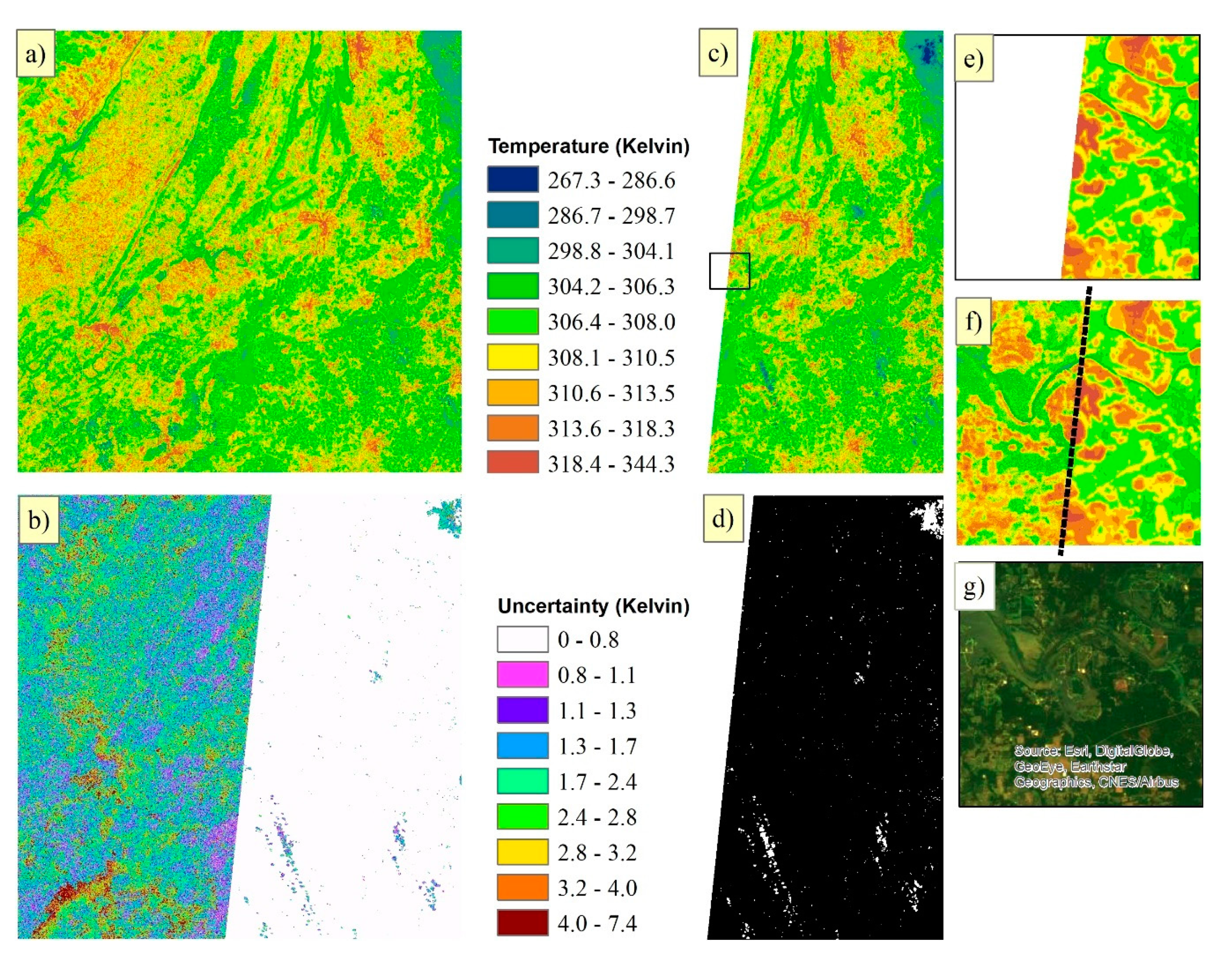
Based on the histogram of clear observations, the minimum value between the two peaks (overlap and non-overlap region) was selected as the threshold (H23V13 > 21, H23V14 > 23, H24V13 > 25, H24V14 > 27). In order to avoid possible boundary issues between tiles, we combined all overlap regions as the training data. Figure 4a shows an example of the model-predicted LST for June 18, 2018, in tile H23V13 for Atlanta. The original Landsat LST only covered the eastern part of the tile (Figure 4c) and was contaminated by scattered clouds (Figure 4d). By closely comparing the two maps, the predicted LST (left side of the dashed line in Figure 4f showed a similar value range to the Landsat LST observations (right side of the dashed line in Figure 4f. Both observations and predictions showed high LST at bare surface and low LST along the river (Figure 4f,g). The spatial distribution is smoother on the left side of Figure 4f than the right side. The uncertainty map (Figure 4b) shows 51.3% of total pixels have the prediction uncertainty less than 4° Kelvin, and 47% of total pixels have valid observations. The spatial pattern of high uncertainty pixels (>4° Kelvin, brown color in Figure 4b matches cloud edge in the 19 July image, where cloud shadows are labeled as clear observations by pixel QA. But the predicted LST does not show those patterns.
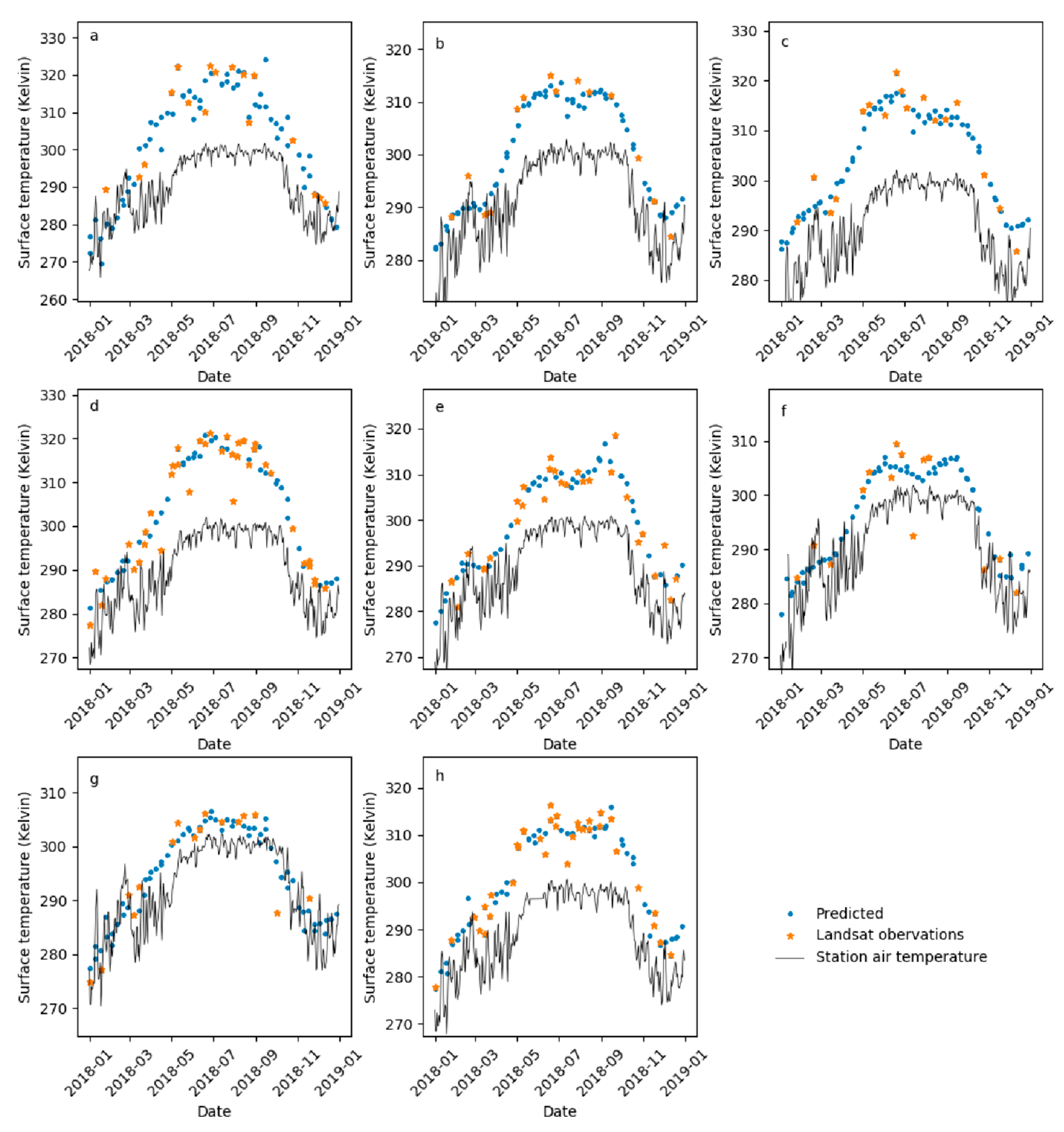
Figure 5 represents the time series of observed and predicted land surface temperature at eight ground station locations in Atlanta. The air temperature is also displayed as a reference of the seasonal temperature pattern at the study area. The predicted values followed well with observations except for several scattered outliers in Figure 5d,f, while both observed and predicted summer LSTs are higher than the station air temperatures. The two outliers in Figure 5d with very low LST came from two Landsat 8 images (26 May 2018 and 29 July 2018) that were mostly covered by clouds, but pixel QA only flagged part of the images as cloud or cloud shadow. Similarly, the low LST at the peak of the summer in Figure 5f also came from a cloud-contaminated observation (Landsat 7 image from 12 July 2018).
5.2. Validation Against the Landsat LST Observations
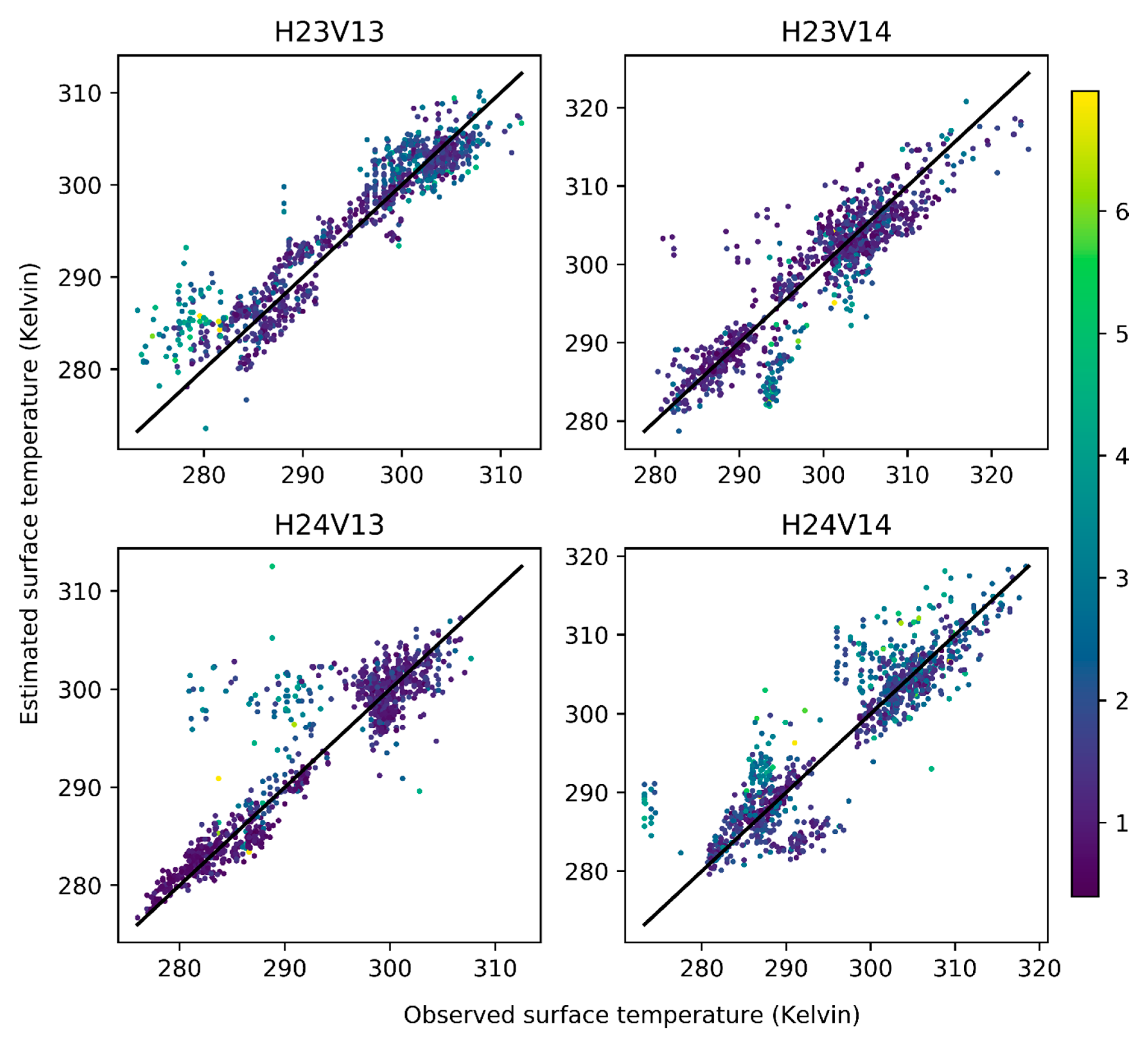
Figure 6 shows the model-estimated LST in relation to 1000 randomly masked clear observations from each tile in Atlanta. All the data in the scatterplots fall close to the 1:1 line, indicating the algorithm can capture the diverse LST caused by seasonality and cover types. In order to assess the accuracy quantitatively, the RMSE and bias (average difference) of observed and predicted LST were calculated (Table 1). The model-estimated LST has a similar range of RMSE and bias compared to the Landsat LST product accuracy, indicating the algorithms have successfully predicted the LST. The dot colors in Figure 6 represent the standard deviation of predictions. Those predictions with high uncertainty or observations distant from the linear relationship mostly occurred at low temperature observations that might come from cloud-contaminated observations that were labeled as clear by pixel QA.
5.3. Gap-Filled Surface Reflectance
Figure 7a,d shows examples of ARD surface reflectance on June 5 and June 6, respectively, using the true color combination. Figure 7b,e are gap-filled images with uncertainty maps of the red band shown in panels (c) and (f). Differing from the LST gap-filled map (Figure 4), there are no visible boundaries between the raw and gap-filled pixels. Some black spots, however, occur in panel (b) because those cloud shadow pixels are flagged as clear or water observation in the pixel QA. The uncertainty maps show there is 55% valid observation plus 45% pixel uncertainty of less than 0.1 in the June 5 image (Figure 7b), and 73% valid observation plus 27% pixel uncertainty of less than 0.1 in the June 6 image (Figure 7f).
The validation shows that the estimated surface reflectance closely matches the actual observations (1:1 line) (Figure 8). Some estimations show large variation while observations are consistent at low or high values in visible bands. As those validation data were randomly picked during the process, it is impossible to examine their condition. However, we went through all 175 gap-filled images and found cloud or cloud shadows were sometimes labeled as clear observation by the Landsat pixel QA band, which could lead to the consistently high or low values at the visible bands. The cloud impact also occurred at shortwave infrared (SWIR) bands as negative values. For all six bands, the majority of RMSEs are less than 0.04 and all biases was less than 0.003 (Table 2). We also conducted t-tests (Table 2) that evaluated whether the predicted values were significantly different from the observations. As p-values suggested, the prediction and observations had no significant difference at the 1% level, though they tended to differ in bands with a small value range.
6. Discussion
Filling data gaps and reducing the variation of data availability is essential for common time series studies [18,22]. Many gap-filling approaches have been developed to fill missing data [22,23,24,25,26], but gap filling in large areas is often challenging using those approaches, especially in heterogeneous regions [8]. This paper presents an effective method to fill gaps in the Landsat ARD products. We used clustering analysis to find orbit overlap region pixels with similar time series to the given pixel and used LASSO regression to estimate their weights. More importantly, we iteratively predicted values using multiple random selections of pixels, which reduced the potential impacts of noise in training data and allowed us to estimate the uncertainty of model predictions. The model uncertainty revealed the stability of model predictions instead of the prediction error. Qualitatively, the results for predicted LST are promising when compared to the spatial patterns of the high-resolution image (Figure 4). The predicted LST showed more spatial detail and variation than LST observations because the raw LST product was resampled to 30-m from 60-m Landsat 7 and 100-m Landsat 8 while the gap-filling procedure was conducted at the 30-m scale. Temporally, the gap-filled data revealed more detailed seasonal variation (Figure 5), which was also confirmed by Yan and Roy [38].
Quantitative validations were undertaken to gain insights into the LST prediction accuracy. Randomly masked 1000 LST observations were compared to model-estimated LST for each tile. The average −0.37 bias and 3.88 RMSE was comparable to the LST product bias (RMSE) of 0.7 K (2.2 K) and 0.9 K (2.3 K) for the four surface radiation budget network sites [32]. For all six spectral bands, the majority of RMSEs were less than 0.04 and all biases were less than 0.0023. In contrast, the MODIS fusion method spatial and temporal adaptive reflectance fusion model (STARFM) had prediction biases of 0.0026 (green band), 0.0040 (red band), and 0.0060 (NIR band) [4]. The enhanced spatial and temporal adaptive reflectance fusion model (ESTARFM) had prediction biases of 0.0028 (green band), 0.0021 (red band), and 0.0022 (NIR band) [4]. Some cloud-contaminated observations were labeled as clear by pixel QA (Figure 8), which could lead to the overestimation of RMSE in both LST and surface reflectance bands in this study.
Some concerns need further investigation. The first concern is data gaps in the overlap region, which could also be considerable. For the current study areas and target time, the number of clear observations (>21) within a year is enough to generate seven-parameter harmonic models for all four Atlanta tiles. According to Egorov et al. [21], the average annual numbers of clear observations are 4.85 (Landsat 4 TM), 16.41 (Landsat 5 TM), 15.03 (Landsat 7 ETM+), and 21.22 (all three Landsat sensors) across the contiguous United States. Therefore, it could be challenging to model observations before 1999 when only one Landsat sensor was available, or for areas with frequent cloud cover or snow cover. An alternative solution is to use the five-parameter nonlinear harmonic model, which needs at least 15 clear observations [22]. Another concern is abrupt changes and short-term changes in data gaps. Conceptually, predicting those changes relies on whether they are captured by training data. But the temporal fitting in the training data may overlook abrupt changes [8]. Using auxiliary data such as climate information or MODIS LST may help avoid the issue. For example, Zhu et al. [5] attempted to predict the changes by fusing MODIS data.
With more and more sensors (e.g., Landsat, Sentinel-2) harmonized, characterizing landscape dynamics at high spatiotemporal resolution attracts groundbreaking attention. However, it also causes complicated data availability variance, while the most traditional time series analysis was designed for data with the same data availability. Our approach attempts to solve the issue, which could be a critical preprocessing step for many time series analyses. Our approach makes the most of original Landsat observations from the same acquisition date, and its cloud-contaminated training data is robust. The current approach used 20 clusters, 100 random samples for each of the 10 iterations, which can be customized according to the computation efficiency. The source code will be available at the GitHub. Finally, Landsat ARD were used in this study for availability and validation convenience, but the approach can be easily applied to another dataset and other vegetation indexes or spectral reflectance bands.
7. Conclusions
This paper presents the results of a new method of time series gap filling that is designed for multi-sensor and multi-time data harmonization. This method uses pixels from the orbit overlap region to fill data gaps based on time series similarity, which retains the observation variation. Model assembling procedures were used to estimate stable predictions, which is not only robust to occasionally cloud-contaminated training data, but also allowed us to estimate the uncertainty of the predictions.
The LST from four ARD tiles (5000 × 5000 30-m pixels for each tile) for Atlanta, Georgia, was tested and validated; the tiles contained heterogeneous land cover types and various temporal variations. The validation procedure suggested good linear relationships with 1000 randomly masked clear observations. More importantly, the application on spectral bands in Fairbanks, Alaska, showed that this approach can effectively fill data gaps related to cloud contamination and sensor orbit models. The gap-filled time series can be of help with reliable seasonal modeling and reducing artifacts related to data availability.
Author Contributions
Conceptualization, G.X., Q.Z.; Methodology, Q.Z.; Supervision, G.X.; Data, H.S.; Writing – original draft, Q.Z.; Writing – review & editing, G.X., H.S. All authors have read and agreed to the published version of the manuscript.
Funding
This research received no external funding.
Acknowledgments
We thank the associate editor and the three anonymous reviewers who helped us substantially improve the manuscript.
Conflicts of Interest
The authors declare no conflict of interest.
Statement
Any use of trade, firm, or product names is for descriptive purposes only and does not imply endorsement by the U.S. Government.
References
- Roy, D.P.; Wulder, M.A.; Loveland, T.R.; Woodcock, C.; Allen, R.G.; Anderson, M.C.; Helder, D.; Irons, J.R.; Johnson, D.M.; Kennedy, R. Landsat-8: Science and product vision for terrestrial global change research. Remote Sens. Environ. 2014, 145, 154–172. [Google Scholar]
- Wulder, M.A.; Masek, J.G.; Cohen, W.B.; Loveland, T.R.; Woodcock, C.E. Opening the archive: How free data has enabled the science and monitoring promise of Landsat. Remote Sens. Environ. 2012, 122, 2–10. [Google Scholar]
- Gao, F.; Masek, J.; Schwaller, M.; Hall, F. On the blending of the Landsat and MODIS surface reflectance: Predicting daily Landsat surface reflectance. IEEE Trans. Geosci. Remote Sens. 2006, 44, 2207–2218. [Google Scholar]
- Zhu, X.; Chen, J.; Gao, F.; Chen, X.; Masek, J.G. An enhanced spatial and temporal adaptive reflectance fusion model for complex heterogeneous regions. Remote Sens. Environ. 2010, 114, 2610–2623. [Google Scholar]
- Zhu, X.; Helmer, E.H.; Gao, F.; Liu, D.; Chen, J.; Lefsky, M.A. A flexible spatiotemporal method for fusing satellite images with different resolutions. Remote Sens. Environ. 2016, 172, 165–177. [Google Scholar]
- Chen, B.; Huang, B.; Xu, B. Comparison of spatiotemporal fusion models: A review. Remote Sens. 2015, 7, 1798–1835. [Google Scholar]
- Gao, F.; Hilker, T.; Zhu, X.; Anderson, M.; Masek, J.; Wang, P.; Yang, Y. Fusing Landsat and MODIS data for vegetation monitoring. IEEE Geosci. Remote Sens. Mag. 2015, 3, 47–60. [Google Scholar]
- Yan, L.; Roy, D. Large-area gap filling of Landsat reflectance time series by spectral-angle-mapper based spatio-temporal similarity (SAMSTS). Remote Sens. 2018, 10, 609. [Google Scholar]
- Gorelick, N.; Hancher, M.; Dixon, M.; Ilyushchenko, S.; Thau, D.; Moore, R. Google Earth Engine: Planetary-scale geospatial analysis for everyone. Remote Sens. Environ. 2017, 202, 18–27. [Google Scholar]
- Claverie, M.; Ju, J.; Masek, J.G.; Dungan, J.L.; Vermote, E.F.; Roger, J.-C.; Skakun, S.V.; Justice, C. The Harmonized Landsat and Sentinel-2 surface reflectance data set. Remote Sens. Environ. 2018, 219, 145–161. [Google Scholar]
- Dwyer, J.; Roy, D.; Sauer, B.; Jenkerson, C.; Zhang, H.; Lymburner, L. Analysis ready data: Enabling analysis of the Landsat archive. Remote Sens. 2018, 10, 1363. [Google Scholar]
- Cook, M.; Schott, J.; Mandel, J.; Raqueno, N. Development of an operational calibration methodology for the Landsat thermal data archive and initial testing of the atmospheric compensation component of a Land Surface Temperature (LST) product from the archive. Remote Sens. 2014, 6, 11244–11266. [Google Scholar]
- Cook, M.J. Atmospheric Compensation for a Landsat Land Surface Temperature Product. Ph.D. Thesis, Rochester Institute of Technology, Rochester, NY, USA, 2014. [Google Scholar]
- Jones, J.W. Improved automated detection of subpixel-scale inundation—Revised dynamic surface water extent (dswe) partial surface water tests. Remote Sens. 2019, 11, 374. [Google Scholar]
- Painter, T.H.; Rittger, K.; McKenzie, C.; Slaughter, P.; Davis, R.E.; Dozier, J. Retrieval of subpixel snow covered area, grain size, and albedo from MODIS. Remote Sens. Environ. 2009, 113, 868–879. [Google Scholar]
- Hawbaker, T.; Vanderhoof, M.; Beal, Y.; Takacs, J.; Schmidt, G.; Falgout, J.; Williams, B.; Fairaux, N.; Caldwell, M.; Picotte, J. Landsat burned area essential climate variable products for the conterminous United States (1984–2015). US Geol. Surv. Data Release 2017, 10, F73B75X76. [Google Scholar]
- Hawbaker, T.J.; Vanderhoof, M.K.; Beal, Y.-J.; Takacs, J.D.; Schmidt, G.L.; Falgout, J.T.; Williams, B.; Fairaux, N.M.; Caldwell, M.K.; Picotte, J.J. Mapping burned areas using dense time-series of Landsat data. Remote Sens. Environ. 2017, 198, 504–522. [Google Scholar]
- Brown, J.F.; Tollerud, H.J.; Barber, C.P.; Zhou, Q.; Dwyer, J.L.; Vogelmann, J.E.; Loveland, T.R.; Woodcock, C.E.; Stehman, S.V.; Zhu, Z. Lessons learned implementing an operational continuous United States national land change monitoring capability: The Land Change Monitoring, Assessment, and Projection (LCMAP) approach. Remote Sens. Environ. 2020, 238, 111356. [Google Scholar]
- Pengra, B.W.; Stehman, S.V.; Horton, J.A.; Dockter, D.J.; Schroeder, T.A.; Yang, Z.; Cohen, W.B.; Healey, S.P.; Loveland, T.R. Quality control and assessment of interpreter consistency of annual land cover reference data in an operational national monitoring program. Remote Sens. Environ. 2020, 238, 111261. [Google Scholar]
- Zhu, Z.; Woodcock, C.E. Continuous change detection and classification of land cover using all available Landsat data. Remote Sens. Environ. 2014, 144, 152–171. [Google Scholar]
- Egorov, A.V.; Roy, D.P.; Zhang, H.K.; Li, Z.; Yan, L.; Huang, H. Landsat 4, 5 and 7 (1982 to 2017) Analysis Ready Data (ARD) observation coverage over the conterminous United States and implications for terrestrial monitoring. Remote Sens. 2019, 11, 447. [Google Scholar]
- Roy, D.; Yan, L. Robust Landsat-based crop time series modelling. Remote Sens. Environ. 2020, 238, 110810. [Google Scholar]
- Chen, J.; Zhu, X.; Vogelmann, J.E.; Gao, F.; Jin, S. A simple and effective method for filling gaps in Landsat ETM+ SLC-off images. Remote Sens. Environ. 2011, 115, 1053–1064. [Google Scholar]
- Lin, C.-H.; Tsai, P.-H.; Lai, K.-H.; Chen, J.-Y. Cloud removal from multitemporal satellite images using information cloning. IEEE Trans. Geosci. Remote Sens. 2012, 51, 232–241. [Google Scholar]
- Schmidt, M.; Pringle, M.; Devadas, R.; Denham, R.; Tindall, D. A framework for large-area mapping of past and present cropping activity using seasonal Landsat images and time series metrics. Remote Sens. 2016, 8, 312. [Google Scholar]
- Zhu, X.; Liu, D.; Chen, J. A new geostatistical approach for filling gaps in Landsat ETM+ SLC-off images. Remote Sens. Environ. 2012, 124, 49–60. [Google Scholar]
- Song, X.-P.; Potapov, P.V.; Krylov, A.; King, L.; Di Bella, C.M.; Hudson, A.; Khan, A.; Adusei, B.; Stehman, S.V.; Hansen, M.C. National-scale soybean mapping and area estimation in the United States using medium resolution satellite imagery and field survey. Remote Sens. Environ. 2017, 190, 383–395. [Google Scholar]
- Weiss, D.J.; Atkinson, P.M.; Bhatt, S.; Mappin, B.; Hay, S.I.; Gething, P.W. An effective approach for gap-filling continental scale remotely sensed time-series. ISPRS J. Photogramm. Remote Sens. 2014, 98, 106–118. [Google Scholar]
- NOAA National Centers for Environmental Information. Climate at a Glance: Global Mapping, August 2019 ed.; NOAA National Centers for Environmental Information: Asheville, NC, USA, 2019.
- Homer, C.; Dewitz, J.; Yang, L.; Jin, S.; Danielson, P.; Xian, G.; Coulston, J.; Herold, N.; Wickham, J.; Megown, K. Completion of the 2011 National Land Cover Database for the conterminous United States—Representing a decade of land cover change information. Photogramm. Eng. Remote Sens. 2015, 81, 345–354. [Google Scholar]
- Yang, L.; Jin, S.; Danielson, P.; Homer, C.; Gass, L.; Bender, S.M.; Case, A.; Costello, C.; Dewitz, J.; Fry, J. A new generation of the United States National Land Cover Database: Requirements, research priorities, design, and implementation strategies. ISPRS J. Photogramm. Remote Sens. 2018, 146, 108–123. [Google Scholar]
- Malakar, N.K.; Hulley, G.C.; Hook, S.J.; Laraby, K.; Cook, M.; Schott, J.R. An operational land surface temperature product for Landsat thermal data: Methodology and validation. IEEE Trans. Geosci. Remote Sens. 2018, 56, 5717–5735. [Google Scholar]
- Zhou, Q.; Liu, S.; Hill, M.J. A Novel Method for Separating Woody and Herbaceous Time Series. Photogramm. Eng. Remote Sens. 2019, 85, 509–520. [Google Scholar]
- Ho, T.K. Random Decision Forests. In Proceedings of the 3rd International Conference on Document Analysis and Recognition, Montreal, QC, Canada, 14–16 August 1995; pp. 278–282. [Google Scholar]
- Arthur, D.; Vassilvitskii, S. k-means++: The advantages of careful seeding. Stanford 2006. [Google Scholar]
- Tibshirani, R. Regression shrinkage and selection via the lasso. J. R. Stat. Soc. Ser. B (Methodol.) 1996, 58, 267–288. [Google Scholar]
- Menne, M.J.; Durre, I.; Korzeniewski, B.; McNeal, S.; Thomas, K.; Yin, X.; Anthony, S.; Ray, R.; Vose, R.S.; Gleason, B.E. Global historical climatology network-daily (GHCN-Daily), Version 3. NOAA Natl. Clim. Data Cent. 2012, 10, V5D21VHZ. [Google Scholar]
- Yan, L.; Roy, D.P. Spatially and temporally complete Landsat reflectance time series modelling: The fill-and-fit approach. Remote Sens. Environ. 2020, 241, 111718. [Google Scholar]
Figure 1.
The first study area is Atlanta, Georgia. Panel (a) shows land cover types from National Land Cover Database (NLCD) 2016. The black lines are boundaries of the four Analysis Ready Data (ARD) tiles (Top left: H23V13, top right: H23V14, bottom left: H24V13, bottom right: H24V14). Panel (b) shows the number of clear observations based on the ARD pixel QA band. Panel (c) shows the second study area in Fairbanks, Alaska. The background image is the true color combination of ARD Landsat 8 on July 6, 2017. Panel (d) shows the Landsat acquisition dates in each tile.

Figure 2.
Illustration of the conceptual approach of gap filling. (a) The time series images with non-clear observations masked. (b) The orbit overlap region with a high density of clear observations. (c) The clustered training data depending on time series similarity. (d) Stratified random samples for a target pixel depending on the time series similarity between the target pixel and cluster centers. (e) A regression model built using the clear observations of samples and the target pixel. The gaps in the target pixel are then predicted from the regression model.

Figure 3.
Workflow of the gap-filling algorithm.

Figure 4.
Land surface temperature from June 18, 2018 (Atlanta, GA) (a) predicted in this study and (c) ARD land surface temperature (LST). Panel (b) shows the model uncertainty of predictions. Panel (d) shows the distribution of valid data (black) and cloud (white) based on the Landsat pixel QA band. (Panel (e) and (f) are zoom-in views of (a) and (c), and the black dashed line shows the boundary between the observed and predicted data. Panel (g) is a high-resolution image of the same region from Esri, DigitalGlobe.

Figure 5.
Time series of land surface temperature and air temperature at eight stations in Atlanta, GA. The orange stars are valid Landsat observations, and blue dots are model-predicted values at each Landsat acquisition date. The black lines are station air temperatures [37] (https://www.ncdc.noaa.gov/ghcn-daily-description). The station ID and latitude–longitude are (a): USW00053863(33.875, -84.302); (b): USW00013874(33.630, -84.442); (c): USW00003888(33.779, -84.521); (d): USC00098740(34.579, -83.332); (e): USC00097600(34.245, -85.151); (f): USC00096335(33.454, -84.818); (g): USC00094170(33.284, -83.468); (h): USC00093621(34.301, -83.860).

Figure 6.
Model-estimated land surface temperature compared to the Landsat observations for four tiles in Atlanta, GA. The color suggests the standard deviation of predictions through iterations.
Figure 6.
Model-estimated land surface temperature compared to the Landsat observations for four tiles in Atlanta, GA. The color suggests the standard deviation of predictions through iterations.

Figure 7.
Fairbanks (Alaska) gap-filling example, 689 × 472 30-m pixel area. Panels (a,d) show examples of ARD surface reflectance on 5 June and 6 June, respectively, using the true color combination. Panels (b,e) are gap-filled images with uncertainty maps of the red band shown in panels (c,f).
Figure 7.
Fairbanks (Alaska) gap-filling example, 689 × 472 30-m pixel area. Panels (a,d) show examples of ARD surface reflectance on 5 June and 6 June, respectively, using the true color combination. Panels (b,e) are gap-filled images with uncertainty maps of the red band shown in panels (c,f).

Figure 8.
Scatterplots of the observed (x-axis) and the predicted reflectance (y-axis) for the blue, green, red, and near-infrared, shortwave infrared 1, and shortwave infrared 2 bands.
Figure 8.
Scatterplots of the observed (x-axis) and the predicted reflectance (y-axis) for the blue, green, red, and near-infrared, shortwave infrared 1, and shortwave infrared 2 bands.


Table 1.
Root Mean Square Error (RMSE) and average difference (observed minus predicted) of land surface temperature (Kelvin) for four tiles in Atlanta, Georgia.
Table 1.
Root Mean Square Error (RMSE) and average difference (observed minus predicted) of land surface temperature (Kelvin) for four tiles in Atlanta, Georgia.
| TILE | RMSE | AVERAGE DIFFERENCE (AD) |
|---|---|---|
| H23V13 | 3.21 | −0.79 |
| H23V14 | 4.09 | 0.54 |
| H24V13 | 3.71 | −0.68 |
| H24V14 | 4.49 | −0.56 |
Table 2.
RMSE and average difference (real reflectance minus predicted reflectance) of the blue, green, red, and near-infrared (NIR), shortwave infrared 1 (SWIR1), and shortwave infrared 2 (SWIR2) bands for Fairbanks, Alaska.
Table 2.
RMSE and average difference (real reflectance minus predicted reflectance) of the blue, green, red, and near-infrared (NIR), shortwave infrared 1 (SWIR1), and shortwave infrared 2 (SWIR2) bands for Fairbanks, Alaska.
| BAND | RMSE | AVERAGE DIFFERENCE (AD) | P-VALUE (T-TEST) |
|---|---|---|---|
| BLUE | 0.0261 | −0.0019 | 0.070 |
| GREEN | 0.0224 | 0.0012 | 0.116 |
| RED | 0.0300 | −0.0022 | 0.040 |
| NIR | 0.0621 | −0.0010 | 0.774 |
| SWIR1 | 0.0327 | 0.0002 | 0.906 |
| SWIR2 | 0.0137 | 0.0007 | 0.231 |
© 2020 by the authors. Licensee MDPI, Basel, Switzerland. This article is an open access article distributed under the terms and conditions of the Creative Commons Attribution (CC BY) license (http://creativecommons.org/licenses/by/4.0/).
Share and Cite
MDPI and ACS Style
Zhou, Q.; Xian, G.; Shi, H. Gap Fill of Land Surface Temperature and Reflectance Products in Landsat Analysis Ready Data. Remote Sens. 2020, 12, 1192. https://0-doi-org.brum.beds.ac.uk/10.3390/rs12071192
AMA Style
Zhou Q, Xian G, Shi H. Gap Fill of Land Surface Temperature and Reflectance Products in Landsat Analysis Ready Data. Remote Sensing. 2020; 12(7):1192. https://0-doi-org.brum.beds.ac.uk/10.3390/rs12071192
Chicago/Turabian StyleZhou, Qiang, George Xian, and Hua Shi. 2020. "Gap Fill of Land Surface Temperature and Reflectance Products in Landsat Analysis Ready Data" Remote Sensing 12, no. 7: 1192. https://0-doi-org.brum.beds.ac.uk/10.3390/rs12071192
Note that from the first issue of 2016, this journal uses article numbers instead of page numbers. See further details here.