Identification of Apple Orchard Planting Year Based on Spatiotemporally Fused Satellite Images and Clustering Analysis of Foliage Phenophase

 ,
,  ,
,
Abstract
:
1. Introduction
2. Materials and Methods
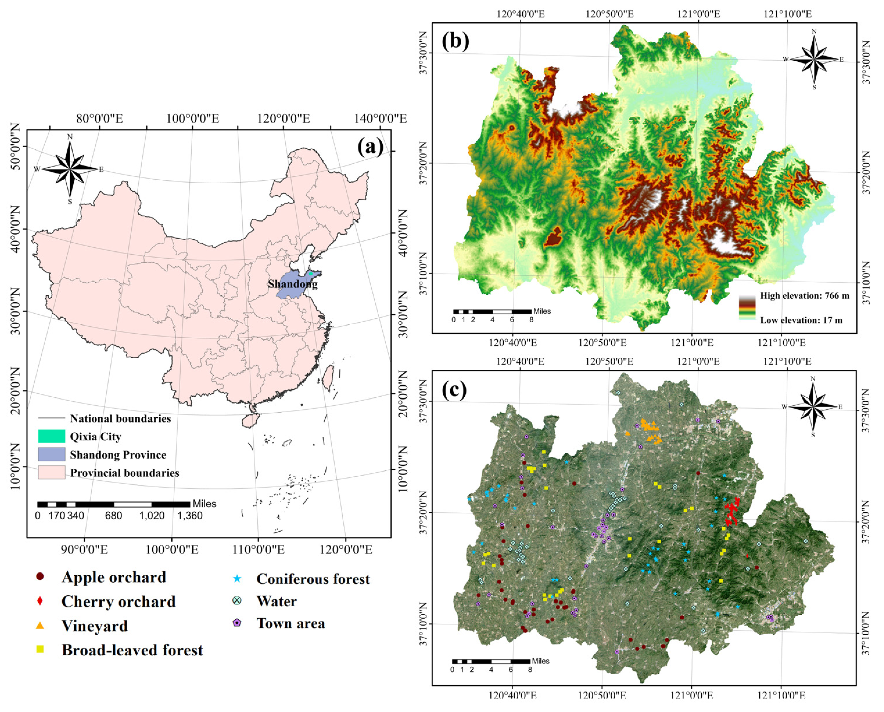
2.1. Study Area
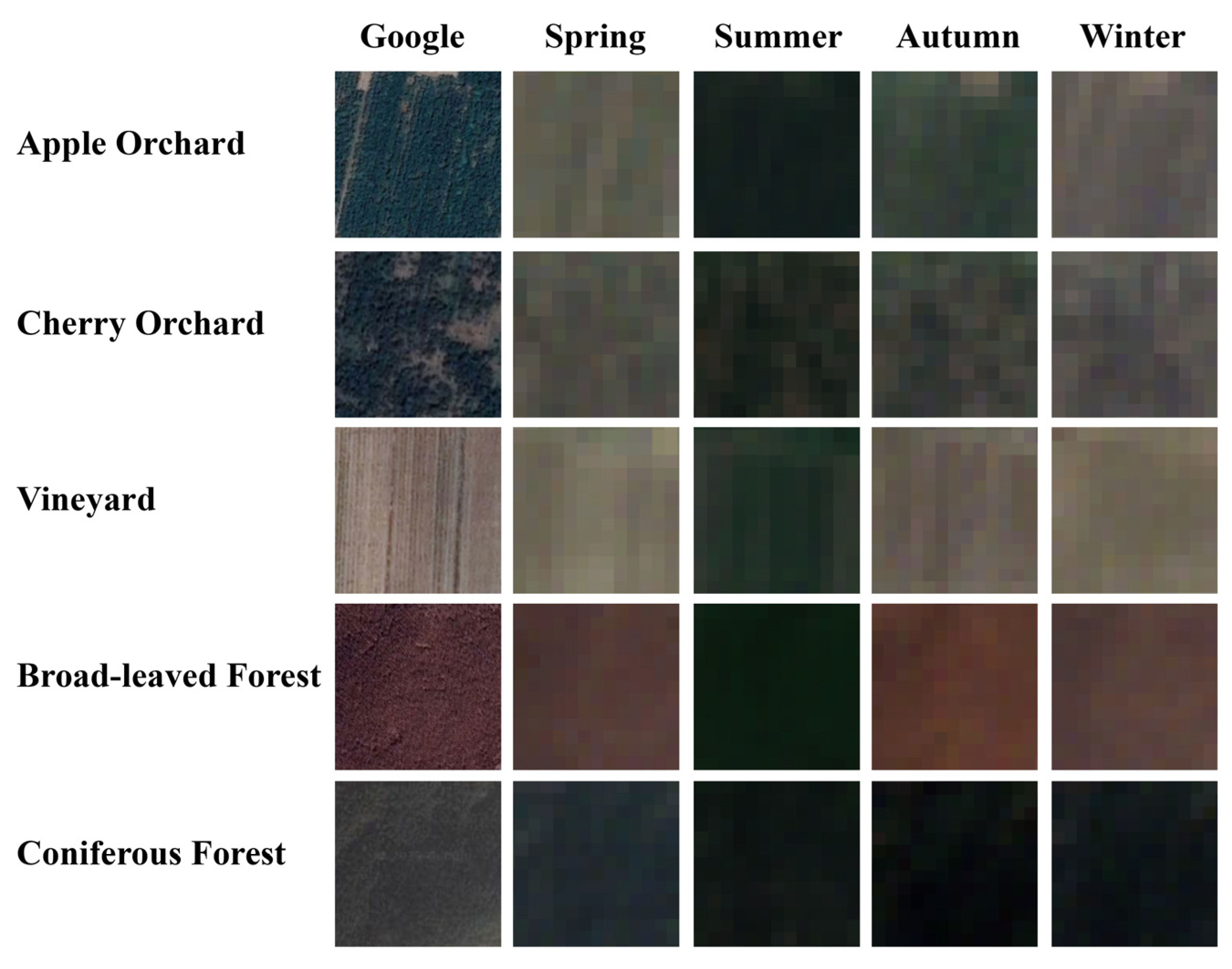
2.2. Field Data
2.3. Remote Sensing Data Acquisition and Preprocessing
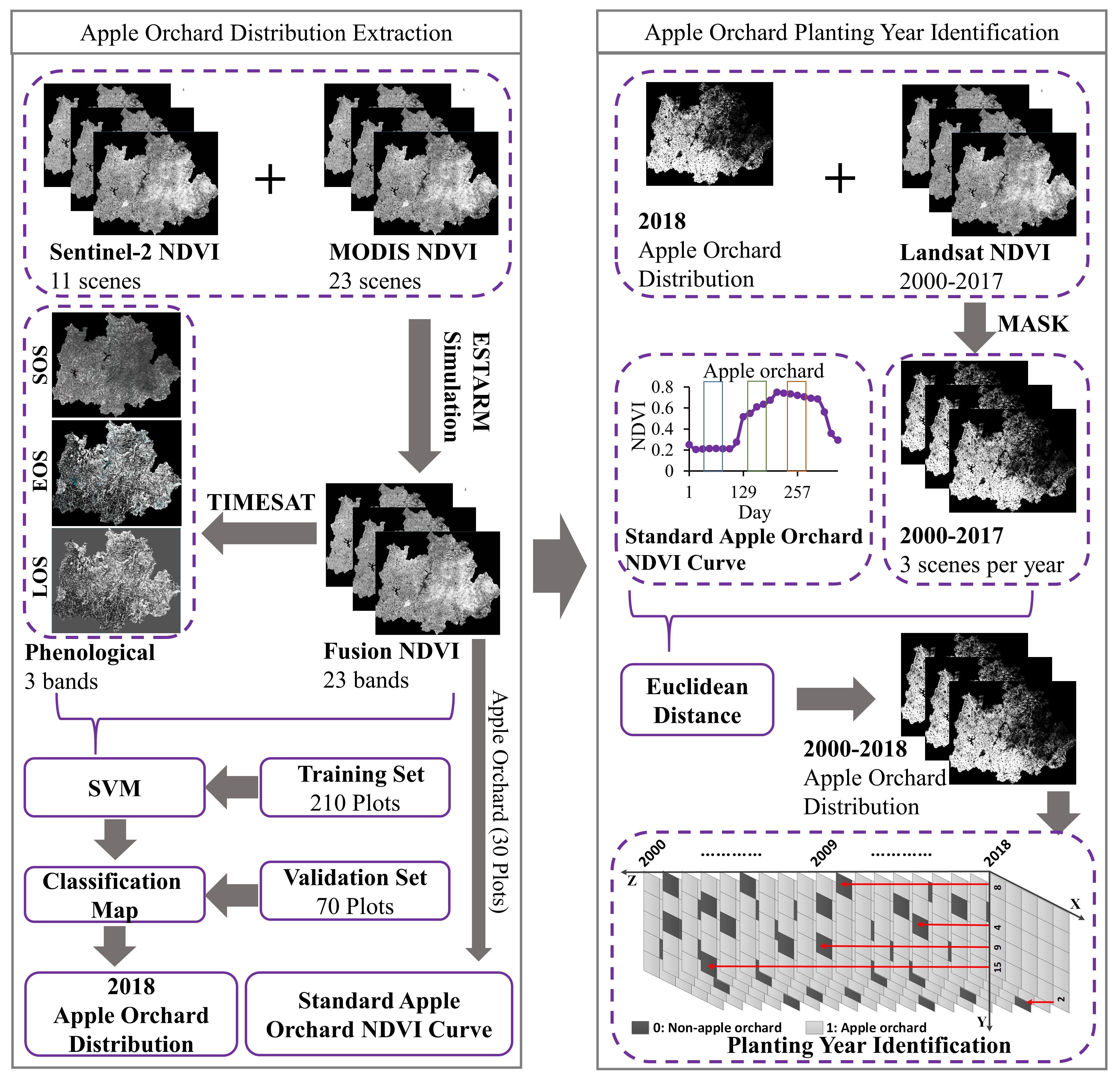
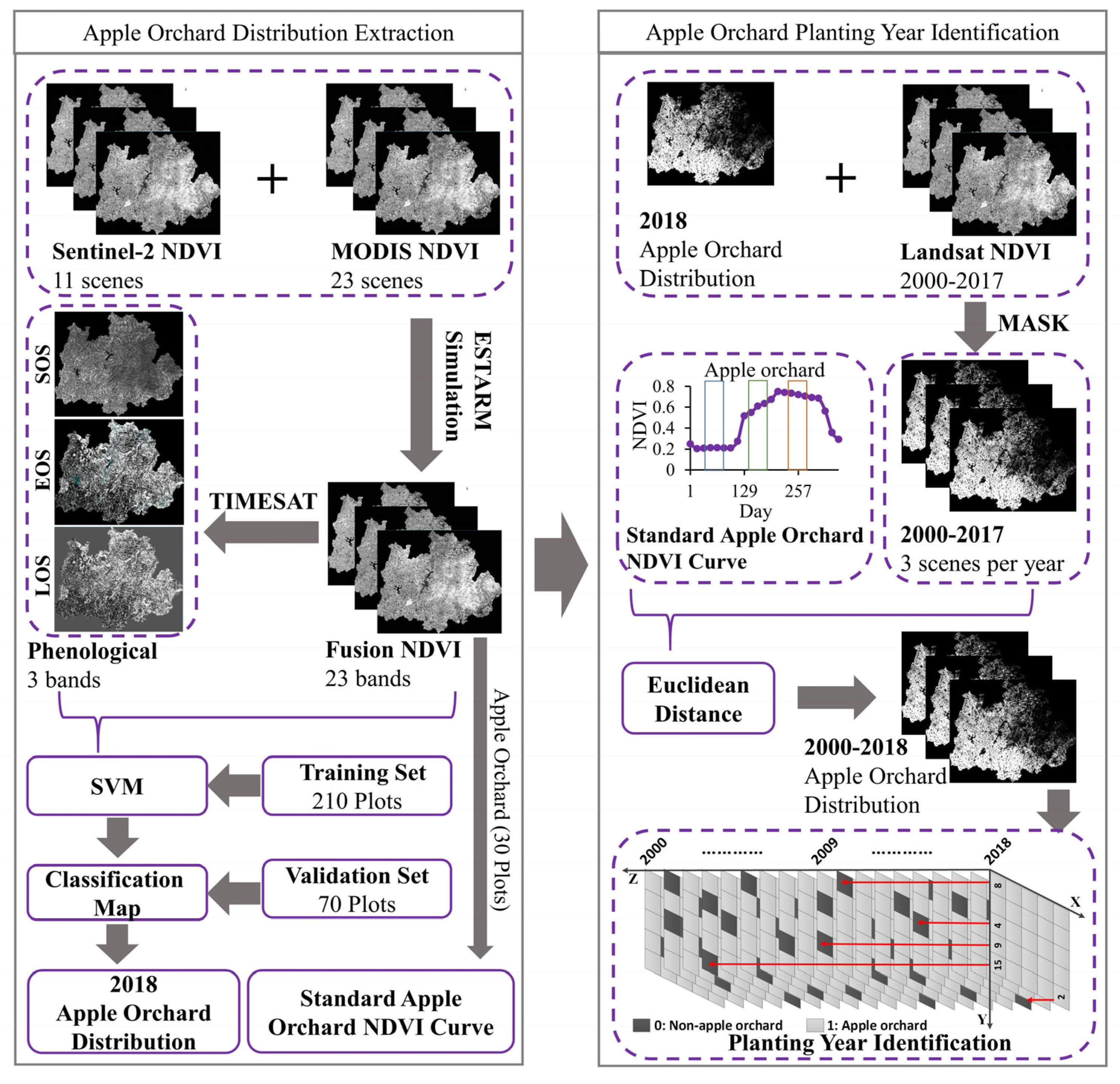
2.4. Identification Method of Apple Orchard Planting Year
- (i)
- Extract the spatial distribution of apple trees. The ESTARFM algorithm is used to fuse the 2018 Sentinel-2 NDVI and MODIS NDVI images to generate a fused NDVI time series. Combined with phenological vegetation features generated using the TIMESAT 3.3 toolbox, an SVM supervised classification method is used to extract the spatial distribution of apple trees. Then, the extracted distribution area of apple trees is used as the region of interest for identifying the planting year;
- (ii)
- Identification of apple orchard planting year. Based on the ROI data of different vegetation types obtained from the field survey, the NDVI time series were extracted from the Sentinel-2/MODIS NDVI spatiotemporally fused images. From the NDVI time-series curves of the apple orchards, three characteristic phenological periods of apple trees were identified, and the NDVI time series of the apple orchards were used as a template to extract the apple orchard distribution area from 2000 to 2017. Then, combined with the Landsat NDVI time-series images composed of three characteristic phenological periods each year from 2000 to 2017 and the apple orchard phenological curve, the apple tree distribution area was calculated for each year between 2000 and 2017 using the ED method, which was run using the MATLAB R2016a software (MathWorks, Natick, MA, USA). Finally, considering the inter-annual changes in apple tree coverage, a pixel-by-pixel inverse time series calculation program developed using the MATLAB software was used to obtain a distribution map of apple orchard planting year for the study region.
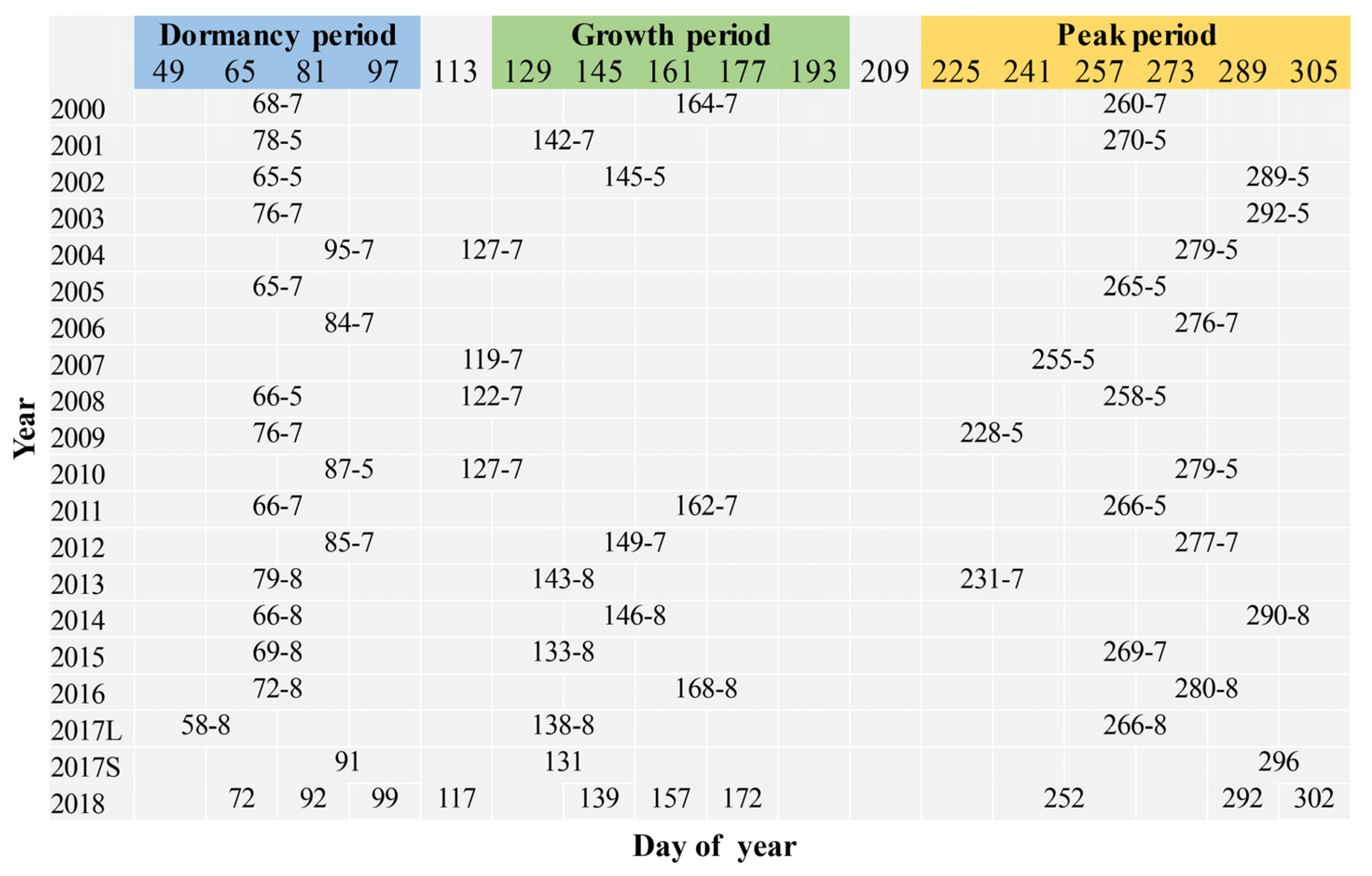
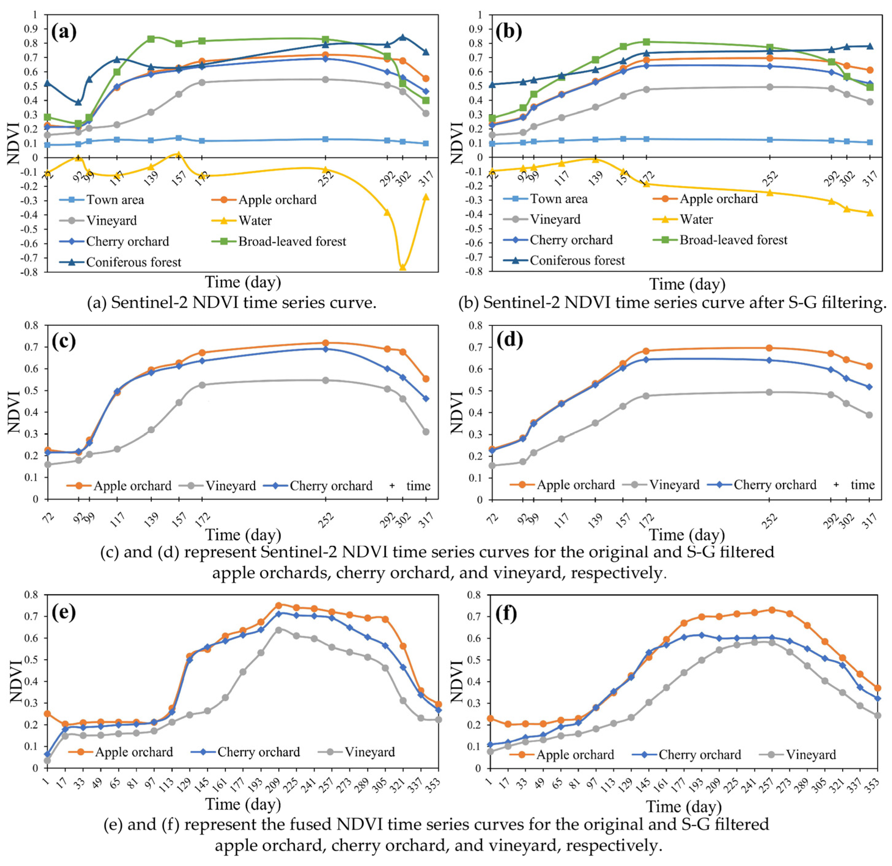
2.4.1. Phenophase Extraction
2.4.2. Land Cover Classification and Accuracy Verification
2.4.3. Determination and Verification of Apple Orchard Planting Year
3. Results
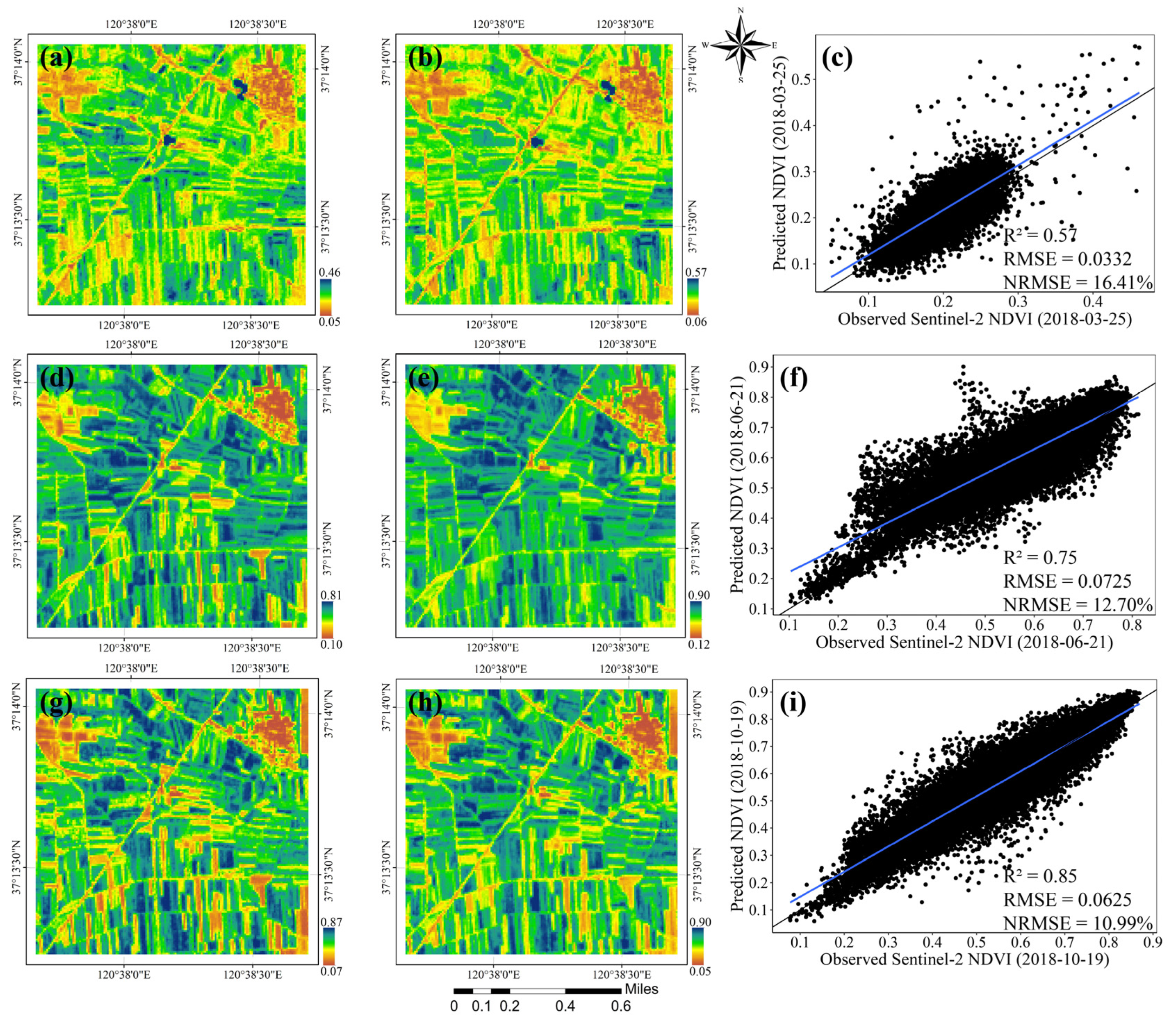
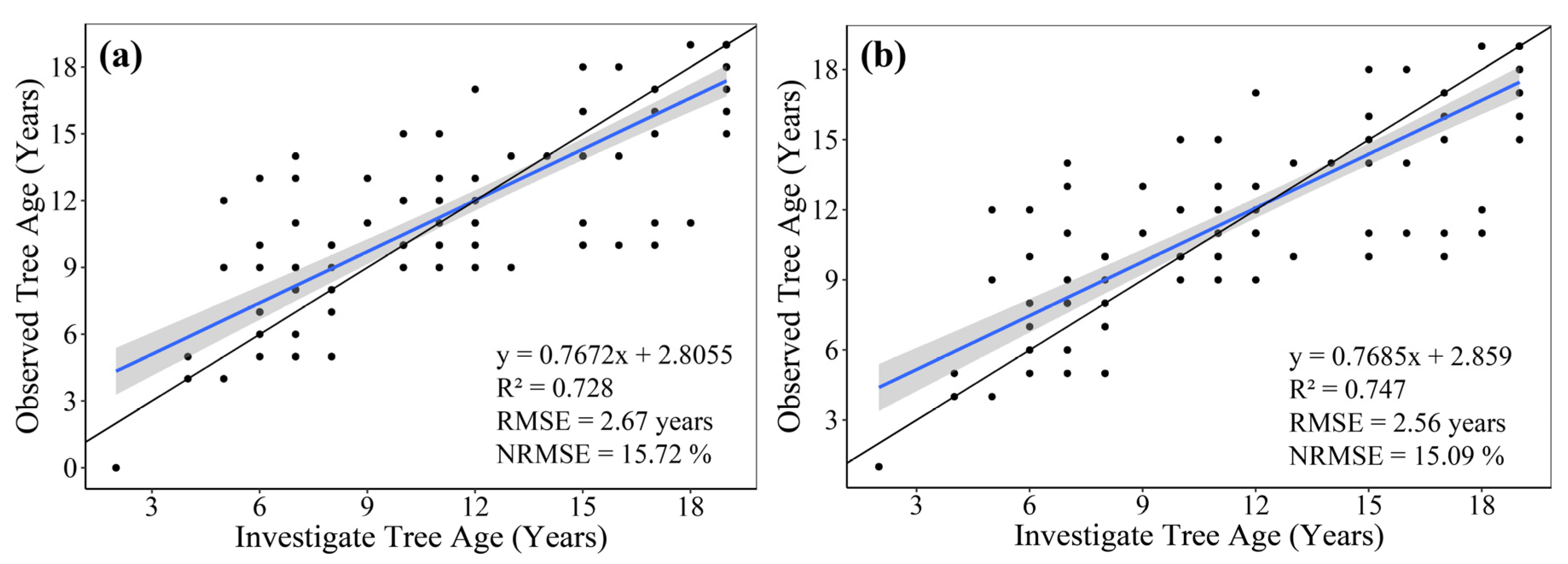
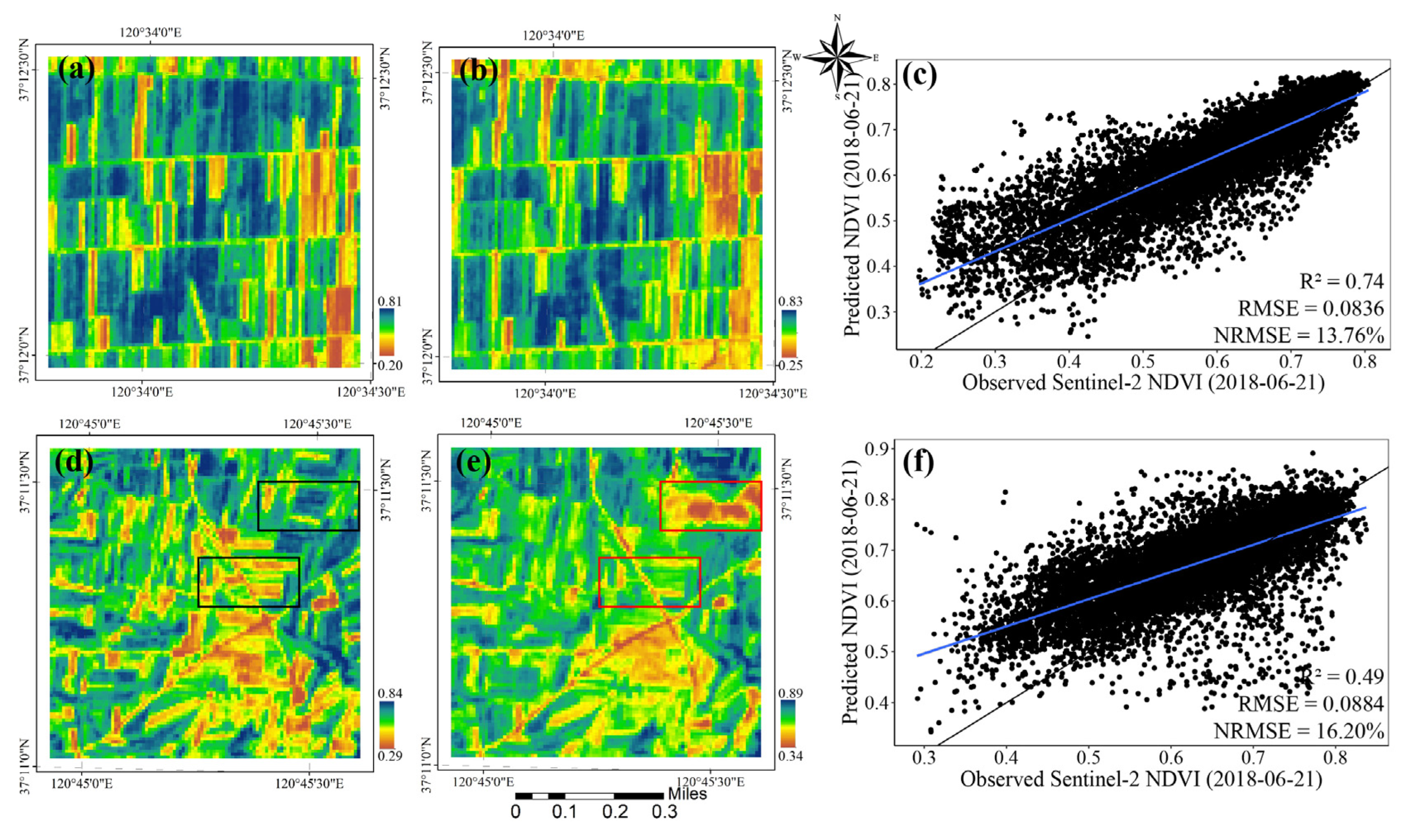
3.1. Validation of the ESTARFM Method
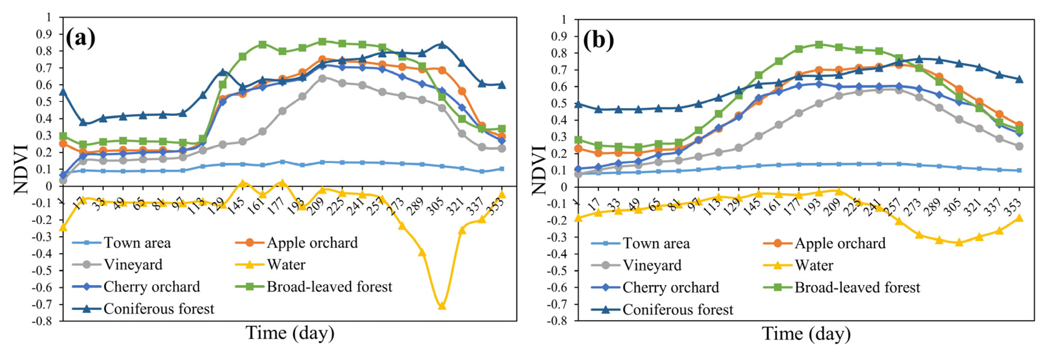
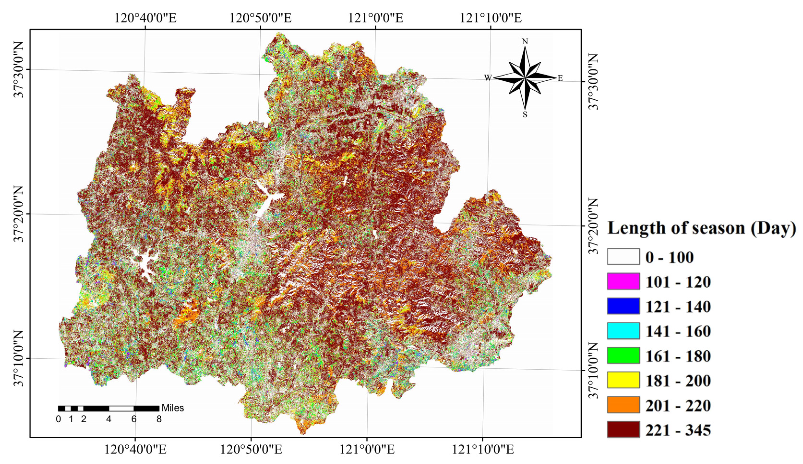
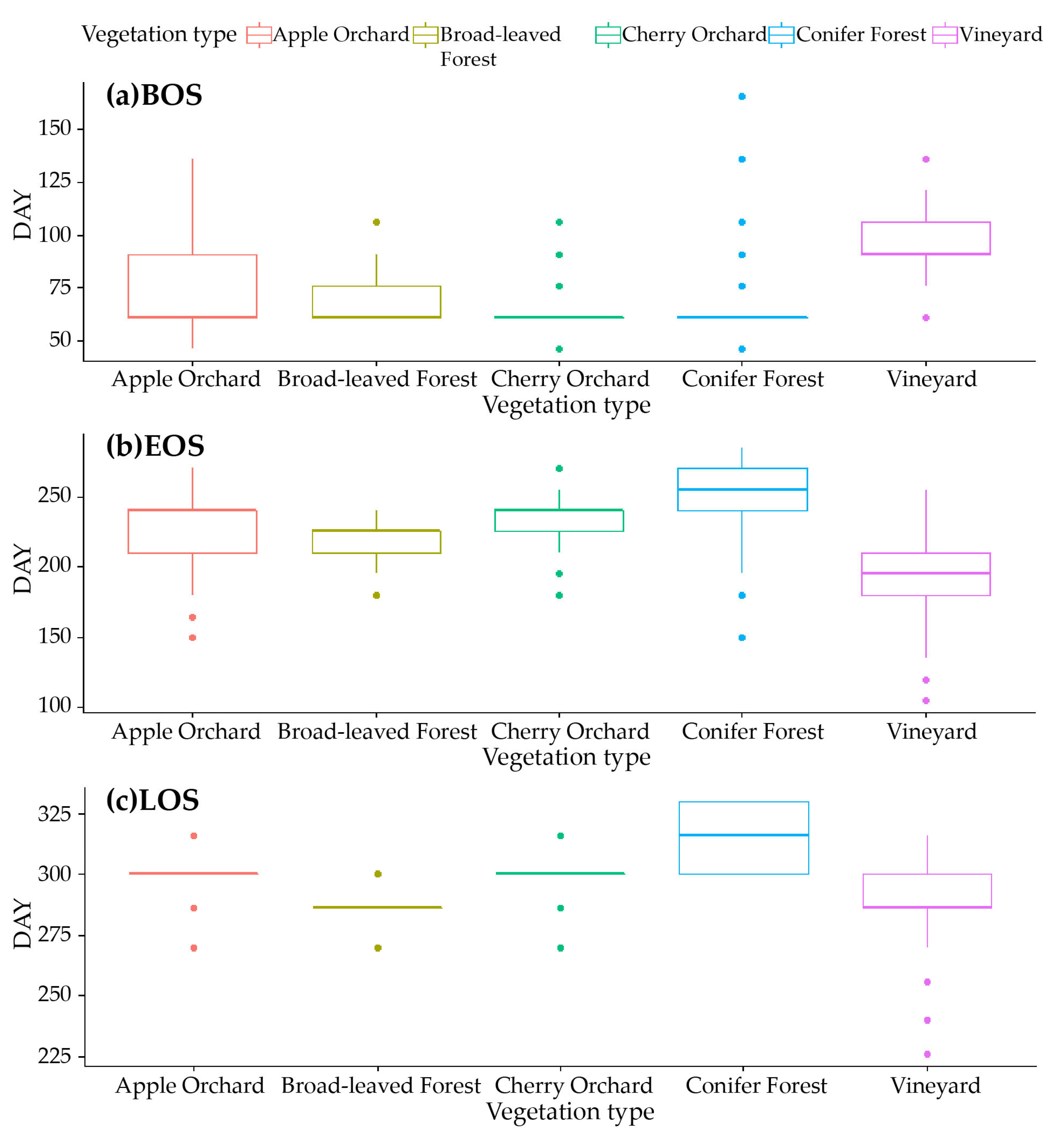
3.2. Extraction of Phenological Information and Analysis
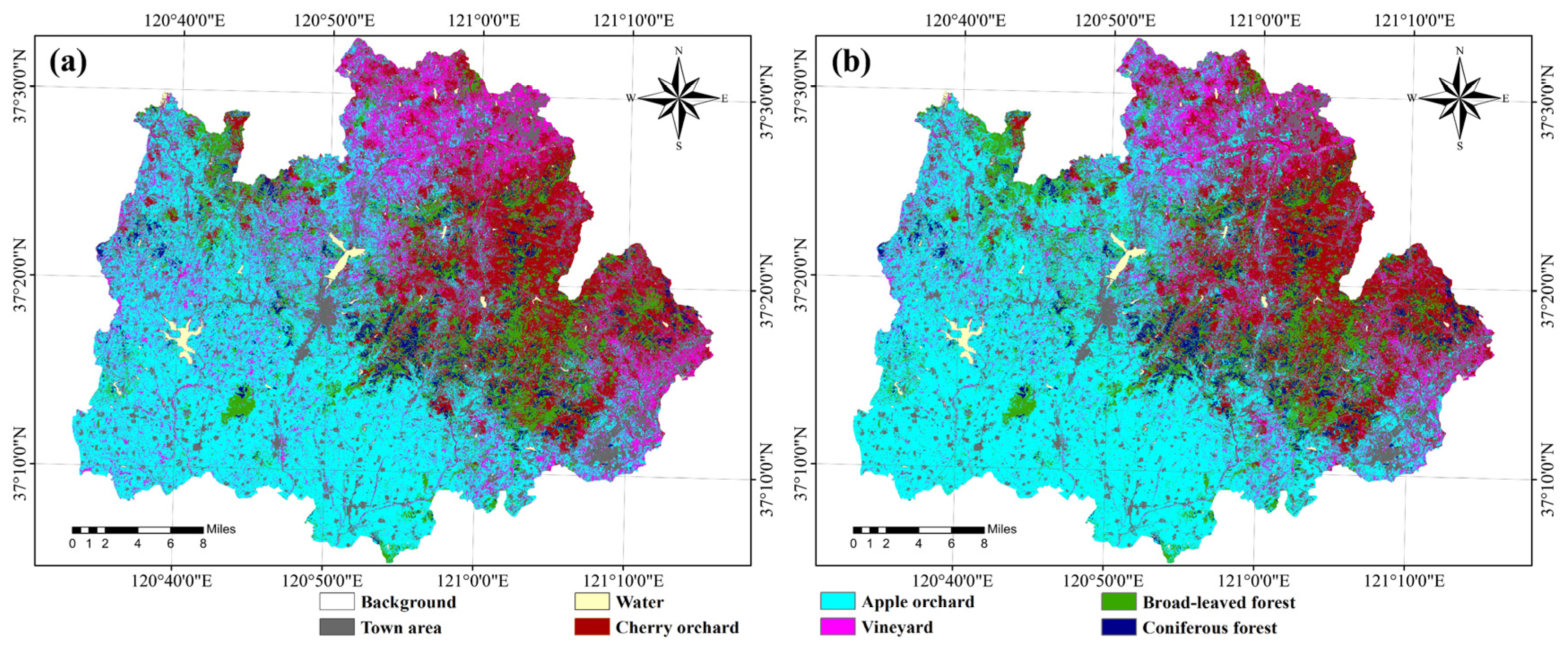
3.3. Classification and Verification
3.4. Extraction of Euclidean Distance and Estimation of Apple Orchard Planting Year
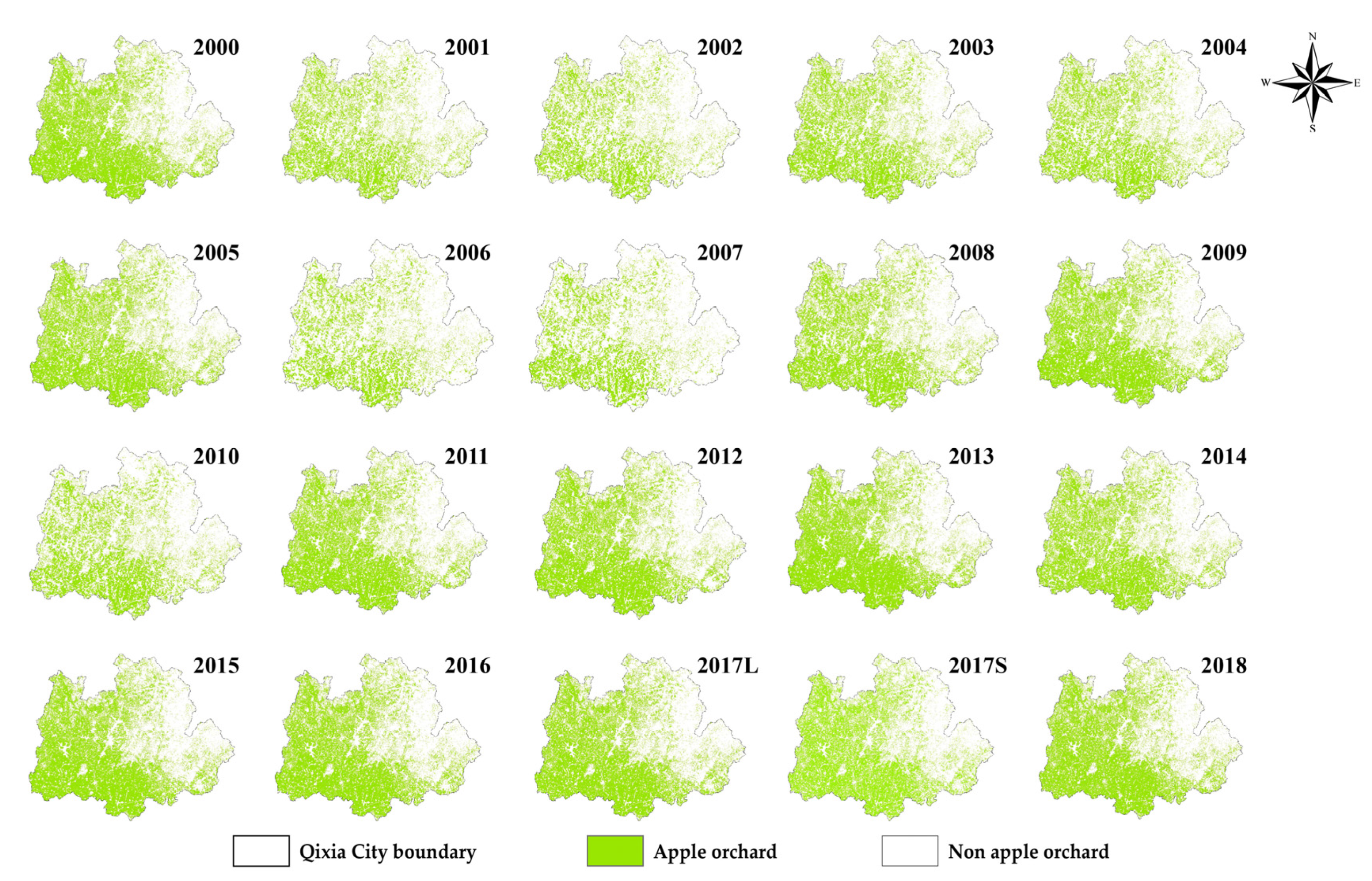
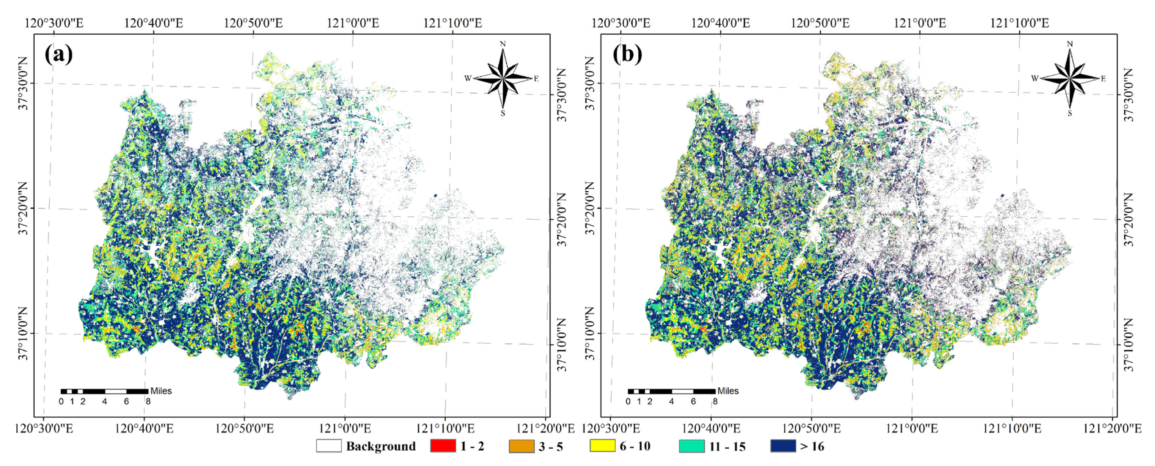
3.5. Apple Orchard Planting Year Extraction and Verification
4. Discussion
4.1. Limitations of the ESTARFM Method
4.2. Method for the Determination of Apple Orchard Planting Year
4.3. Application Prospect of Apple Orchard Planting Year
5. Conclusions
Author Contributions
Funding
Conflicts of Interest
References
- FAO (Food and Agriculture Organization of the United Nations). FAOSTAT Production Database. FAO. 2017. Available online: http://www.fao.org/faostat/zh/#data/QC (accessed on 8 April 2020).
- Chen, B.Q.; Xiao, X.M.; Wu, Z.X.; Yun, T.; Kou, W.L.; Ye, H.C.; Lin, Q.H.; Doughty, R.; Dong, J.W.; Ma, J.; et al. Identifying Establishment Year and Pre-Conversion Land Cover of Rubber Plantations on Hainan Island, China Using Landsat Data during 1987–2015. Remote Sens. 2018, 10. [Google Scholar] [CrossRef] [Green Version]
- Altman, J.; Dolezal, J.; Cizek, L. Age estimation of large trees: New method based on partial increment core tested on an example of veteran oaks. Forest Ecol. Manag. 2016, 380, 82–89. [Google Scholar] [CrossRef]
- Chen, G.; Thill, J.C.; Anantsuksomsri, S.; Tontisirin, N.; Tao, R. Stand age estimation of rubber (Hevea brasiliensis) plantations using an integrated pixel- and object-based tree growth model and annual Landsat time series. ISPRS J. Photogramm. 2018, 144, 94–104. [Google Scholar] [CrossRef]
- Bai, T.C.; Zhang, N.N.; Mercatoris, B.; Chen, Y.Q. Improving Jujube Fruit Tree Yield Estimation at the Field Scale by Assimilating a Single Landsat Remotely-Sensed LAI into the WOFOST Model. Remote Sens. 2019, 11. [Google Scholar] [CrossRef] [Green Version]
- Ou, G.L.; Li, C.; Lv, Y.Y.; Wei, A.C.; Xiong, H.X.; Xu, H.; Wang, G.X. Improving Aboveground Biomass Estimation of Pinus densata Forests in Yunnan Using Landsat 8 Imagery by Incorporating Age Dummy Variable and Method Comparison. Remote Sens. 2019, 11. [Google Scholar] [CrossRef] [Green Version]
- Kozhoridze, G.; Orlovsky, N.; Orlovsky, L.; Blumberg, D.G.; Golan-Goldhirsh, A. Classification-based mapping of trees in commercial orchards and natural forests. Int. J. Remote Sens. 2018, 39, 8784–8797. [Google Scholar] [CrossRef]
- Franklin, S.E.; Hall, R.J.; Smith, L.; Gerylo, G.R. Discrimination of conifer height, age and crown closure classes using Landsat-5 TM imagery in the Canadian Northwest Territories. Int J. Remote Sens. 2003, 24, 1823–1834. [Google Scholar] [CrossRef]
- McMorrow, J. Relation of oil palm spectral response to stand age. Int. J. Remote Sens. 1995, 16, 3203–3209. [Google Scholar] [CrossRef]
- Thenkabail, P.S.; Stucky, N.; Griscom, B.W.; Ashton, M.S.; Diels, J.; Van der Meer, B.; Enclona, E. Biomass estimations and carbon stock calculations in the oil palm plantations of African derived savannas using IKONOS data. Int. J. Remote Sens. 2004, 25, 5447–5472. [Google Scholar] [CrossRef]
- Buddenbaum, H.; Schlerf, M.; Hill, J. Classification of coniferous tree species and age classes using hyperspectral data and geostatistical methods. Int. J. Remote Sens. 2005, 26, 5453–5465. [Google Scholar] [CrossRef]
- Lefsky, M.A.; Turner, D.P.; Guzy, M.; Cohen, W.B. Combining lidar estimates of aboveground biomass and Landsat estimates of stand age for spatially extensive validation of modeled forest productivity. Remote Sens. Environ. 2005, 95, 549–558. [Google Scholar] [CrossRef]
- Hamsa, C.S.; Kanniah, K.D.; Muharam, F.M.; Idris, N.H.; Abdullah, Z.; Mohamed, L. Textural measures for estimating oil palm age. Int. J. Remote Sens. 2019, 40, 7516–7537. [Google Scholar] [CrossRef]
- Chemura, A.; van Duren, I.; van Leeuwen, L.M. Determination of the age of oil palm from crown projection area detected from World View-2 multispectral remote sensing data: The case of Ejisu-Juaben district, Ghana. ISPRS J. Photogramm. 2015, 100, 118–127. [Google Scholar] [CrossRef]
- Vastaranta, M.; Niemi, M.; Wulder, M.A.; White, J.C.; Nurminen, K.; Litkey, P.; Honkavaara, E.; Holopainen, M.; Hyyppa, J. Forest stand age classification using time series of photogrammetrically derived digital surface models. Scand. J. Forest Res. 2016, 31, 194–205. [Google Scholar] [CrossRef] [Green Version]
- Racine, E.B.; Coops, N.C.; St-Onge, B.; Begin, J. Estimating Forest Stand Age from LiDAR-Derived Predictors and Nearest Neighbor Imputation. Forest Sci. 2014, 60, 128–136. [Google Scholar] [CrossRef]
- Iizuka, K.; Tateishi, R. Estimation of CO2 Sequestration by the Forests in Japan by Discriminating Precise Tree Age Category using Remote Sensing Techniques. Remote Sens. 2015, 7, 15082–15113. [Google Scholar] [CrossRef] [Green Version]
- Rizeei, H.M.; Shafri, H.Z.M.; Mohamoud, M.A.; Pradhan, B.; Kalantar, B. Oil Palm Counting and Age Estimation from WorldView-3 Imagery and LiDAR Data Using an Integrated OBIA Height Model and Regression Analysis. J. Sens. 2018. [Google Scholar] [CrossRef] [Green Version]
- Tan, K.P.; Kanniah, K.D.; Cracknell, A.P. Use of UK-DMC 2 and ALOS PALSAR for studying the age of oil palm trees in southern peninsular Malaysia. Int. J. Remote Sens. 2013, 34, 7424–7446. [Google Scholar] [CrossRef]
- Esch, T.; Metz, A.; Marconcini, M.; Keil, M. Combined use of multi-seasonal high and medium resolution satellite imagery for parcel-related mapping of cropland and grassland. Int. J. Appl. Earth Obs. 2014, 28, 230–237. [Google Scholar] [CrossRef]
- Pena, M.A.; Brenning, A. Assessing fruit-tree crop classification from Landsat-8 time series for the Maipo Valley, Chile. Remote Sens. Environ. 2015, 171, 234–244. [Google Scholar] [CrossRef]
- Jia, K.; Liang, S.L.; Wei, X.Q.; Yao, Y.J.; Su, Y.R.; Jiang, B.; Wang, X.X. Land Cover Classification of Landsat Data with Phenological Features Extracted from Time Series MODIS NDVI Data. Remote Sens. 2014, 6, 11518–11532. [Google Scholar] [CrossRef] [Green Version]
- Kong, F.J.; Li, X.B.; Wang, H.; Xie, D.F.; Li, X.; Bai, Y.X. Land Cover Classification Based on Fused Data from GF-1 and MODIS NDVI Time Series. Remote Sens. 2016, 8. [Google Scholar] [CrossRef] [Green Version]
- Yan, J.; Wang, L.; Song, W.; Chen, Y.; Chen, X.; Deng, Z. A time-series classification approach based on change detection for rapid land cover mapping. ISPRS J. Photogramm. 2019, 158, 249–262. [Google Scholar] [CrossRef]
- Salmon, B.P.; Kleynhans, W.; Olivier, J.C.; van den Bergh, F.; Wessels, K.J. A modified temporal criterion to meta-optimize the extended Kalman filter for land cover classification of remotely sensed time series. Int. J. Appl. Earth Obs. 2018, 67, 20–29. [Google Scholar] [CrossRef]
- Gómez, C.; White, J.C.; Wulder, M.A. Optical remotely sensed time series data for land cover classification: A review. ISPRS J. Photogramm. 2016, 116, 55–72. [Google Scholar] [CrossRef] [Green Version]
- Watts, J.D.; Powell, S.L.; Lawrence, R.L.; Hilker, T. Improved classification of conservation tillage adoption using high temporal and synthetic satellite imagery. Remote Sens. Environ. 2011, 115, 66–75. [Google Scholar] [CrossRef]
- Gao, F.; Masek, J.; Schwaller, M.; Hall, F. On the blending of the Landsat and MODIS surface reflectance: Predicting daily Landsat surface reflectance. IEEE Trans. Geosci. Remote 2006, 44, 2207–2218. [Google Scholar] [CrossRef]
- Senf, C.; Leitão, P.J.; Pflugmacher, D.; van der Linden, S.; Hostert, P. Mapping land cover in complex Mediterranean landscapes using Landsat: Improved classification accuracies from integrating multi-seasonal and synthetic imagery. Remote Sens. Environ. 2015, 156, 527–536. [Google Scholar] [CrossRef]
- Zhu, L.K.; Radeloff, V.C.; Ives, A.R. Improving the mapping of crop types in the Midwestern US by fusing Landsat and MODIS satellite data. Int. J. Appl. Earth Obs. 2017, 58, 1–11. [Google Scholar] [CrossRef]
- Heimhuber, V.; Tulbure, M.G.; Broich, M. Addressing spatio-temporal resolution constraints in Landsat and MODIS-based mapping of large-scale floodplain inundation dynamics. Remote Sens. Environ. 2018, 211, 307–320. [Google Scholar] [CrossRef]
- Chen, B.; Chen, L.F.; Huang, B.; Michishita, R.; Xu, B. Dynamic monitoring of the Poyang Lake wetland by integrating Landsat and MODIS observations. ISPRS J. Photogramm. 2018, 139, 75–87. [Google Scholar] [CrossRef]
- Zhu, X.L.; Chen, J.; Gao, F.; Chen, X.H.; Masek, J.G. An enhanced spatial and temporal adaptive reflectance fusion model for complex heterogeneous regions. Remote Sens. Environ. 2010, 114, 2610–2623. [Google Scholar] [CrossRef]
- Ienco, D.; Interdonato, R.; Gaetano, R.; Ho Tong Minh, D. Combining Sentinel-1 and Sentinel-2 Satellite Image Time Series for land cover mapping via a multi-source deep learning architecture. ISPRS J. Photogramm. 2019, 158, 11–22. [Google Scholar] [CrossRef]
- Macintyre, P.; van Niekerk, A.; Mucina, L. Efficacy of multi-season Sentinel-2 imagery for compositional vegetation classification. Int. J. Appl. Earth Obs. 2020, 85, 101980. [Google Scholar] [CrossRef]
- Garcia-Llamas, P.; Suarez-Seoane, S.; Fernandez-Guisuraga, J.M.; Fernandez-Garcia, V.; Fernandez-Manso, A.; Quintano, C.; Taboada, A.; Marcos, E.; Calvo, L. Evaluation and comparison of Landsat 8, Sentinel-2 and Deimos-1 remote sensing indices for assessing burn severity in Mediterranean fire-prone ecosystems. Int. J. Appl. Earth Obs. 2019, 80, 137–144. [Google Scholar] [CrossRef]
- Wittke, S.; Yu, X.W.; Karjalainen, M.; Hyyppa, J.; Puttonen, E. Comparison of two-dimensional multitemporal Sentinel-2 data with three-dimensional remote sensing data sources for forest inventory parameter estimation over a boreal forest. Int. J. Appl. Earth Obs. 2019, 76, 167–178. [Google Scholar] [CrossRef]
- Xie, Q.Y.; Dash, A.D.; Huete, A.R.O.; Jiang, A.H.; Yin, G.F.; Ding, Y.L.; Peng, D.L.; Hall, R.O.E.; Brown, L.K.; Shi, Y.; et al. Retrieval of crop biophysical parameters from Sentinel-2 remote sensing imagery. Int. J. Appl. Earth Obs. 2019, 80, 187–195. [Google Scholar] [CrossRef]
- Battude, M.; Al Bitar, A.; Morin, D.; Cros, J.; Huc, M.; Sicre, C.M.; Le Dantec, V.; Demarez, V. Estimating maize biomass and yield over large areas using high spatial and temporal resolution Sentinel-2 like remote sensing data. Remote Sens. Environ. 2016, 184, 668–681. [Google Scholar] [CrossRef]
- Tucker, C.J. Red and photographic infrared linear combinations for monitoring vegetation. Remote Sens. Environ. 1979, 8, 127–150. [Google Scholar] [CrossRef] [Green Version]
- Roy, D.P.; Wulder, M.A.; Loveland, T.R.; Woodcock, C.E.; Allen, R.G.; Anderson, M.C.; Helder, D.; Irons, J.R.; Johnson, D.M.; Kennedy, R.; et al. Landsat-8: Science and product vision for terrestrial global change research. Remote Sens. Environ. 2014, 145, 154–172. [Google Scholar] [CrossRef] [Green Version]
- Zeng, L.; Wardlow, B.D.; Xiang, D.; Hu, S.; Li, D. A review of vegetation phenological metrics extraction using time-series, multispectral satellite data. Remote Sens. Environ. 2020, 237, 111511. [Google Scholar] [CrossRef]
- Azzari, G.; Lobell, D.B. Landsat-based classification in the cloud: An opportunity for a paradigm shift in land cover monitoring. Remote Sens. Environ. 2017, 202, 64–74. [Google Scholar] [CrossRef]
- Phiri, D.; Morgenroth, J.; Xu, C.; Hermosilla, T. Effects of pre-processing methods on Landsat OLI-8 land cover classification using OBIA and random forests classifier. Int. J. Appl. Earth Obs. 2018, 73, 170–178. [Google Scholar] [CrossRef]
- Berra, E.F.; Gaulton, R.; Barr, S. Assessing spring phenology of a temperate woodland: A multiscale comparison of ground, unmanned aerial vehicle and Landsat satellite observations. Remote Sens. Environ. 2019, 223, 229–242. [Google Scholar] [CrossRef]
- Senf, C.; Pflugmacher, D.; Heurich, M.; Krueger, T. A Bayesian hierarchical model for estimating spatial and temporal variation in vegetation phenology from Landsat time series. Remote Sens. Environ. 2017, 194, 155–160. [Google Scholar] [CrossRef]
- Abd Razak, J.A.B.; Shariff, A.R.B.; bin Ahmad, N.; Sameen, M.I. Mapping rubber trees based on phenological analysis of Landsat time series data-sets. Geocarto Int. 2018, 33, 627–650. [Google Scholar] [CrossRef]
- Xue, Z.H.; Du, P.J.; Feng, L. Phenology-Driven Land Cover Classification and Trend Analysis Based on Long-term Remote Sensing Image Series. IEEE J. Stars 2014, 7, 1142–1156. [Google Scholar] [CrossRef]
- Chen, J.; Jönsson, P.; Tamura, M.; Gu, Z.; Matsushita, B.; Eklundh, L. A simple method for reconstructing a high-quality NDVI time-series data set based on the Savitzky–Golay filter. Remote Sens. Environ. 2004, 91, 332–344. [Google Scholar] [CrossRef]
- Shao, Y.; Lunetta, R.S.; Wheeler, B.; Iiames, J.S.; Campbell, J.B. An evaluation of time-series smoothing algorithms for land-cover classifications using MODIS-NDVI multi-temporal data. Remote Sens. Environ. 2016, 174, 258–265. [Google Scholar] [CrossRef]
- Senf, C.; Pflugmacher, D.; van der Linden, S.; Hostert, P. Mapping Rubber Plantations and Natural Forests in Xishuangbanna (Southwest China) Using Multi-Spectral Phenological Metrics from MODIS Time Series. Remote Sens. 2013, 5, 2795–2812. [Google Scholar] [CrossRef] [Green Version]
- Geiss, C.; Pelizari, P.A.; Blickensdorfer, L.; Taubenbock, H. Virtual Support Vector Machines with self-learning strategy for classification of multispectral remote sensing imagery. ISPRS J. Photogramm. 2019, 151, 42–58. [Google Scholar] [CrossRef]
- Maulik, U.; Chakraborty, D. Learning with transductive SVM for semisupervised pixel classification of remote sensing imagery. ISPRS J. Photogramm. 2013, 77, 66–78. [Google Scholar] [CrossRef]
- Danielsson, P.-E. Euclidean distance mapping. Comput. Graph. Image Process. 1980, 14, 227–248. [Google Scholar] [CrossRef] [Green Version]
- Zhu, Y.H.; Zhao, C.J.; Yang, H.; Yang, G.J.; Han, L.; Li, Z.H.; Feng, H.K.; Xu, B.; Wu, J.T.; Lei, L. Estimation of maize above-ground biomass based on stem-leaf separation strategy integrated with LiDAR and optical remote sensing data. PeerJ 2019, 7. [Google Scholar] [CrossRef] [PubMed] [Green Version]
- Atkinson, P.M.; Jeganathan, C.; Dash, J.; Atzberger, C. Inter-comparison of four models for smoothing satellite sensor time-series data to estimate vegetation phenology. Remote Sens. Environ. 2012, 123, 400–417. [Google Scholar] [CrossRef]
- Guo, L.; Wang, J.; Li, M.; Liu, L.; Xu, J.; Cheng, J.; Gang, C.; Yu, Q.; Chen, J.; Peng, C.; et al. Distribution margins as natural laboratories to infer species’ flowering responses to climate warming and implications for frost risk. Agric. Forest Meteorol. 2019, 268, 299–307. [Google Scholar] [CrossRef]
- White, K.; Pontius, J.; Schaberg, P. Remote sensing of spring phenology in northeastern forests: A comparison of methods, field metrics and sources of uncertainty. Remote Sens. Environ. 2014, 148, 97–107. [Google Scholar] [CrossRef]
- Jonsson, P.; Eklundh, L. TIMESAT—A program for analyzing time-series of satellite sensor data. Comput. Geosci. 2004, 30, 833–845. [Google Scholar] [CrossRef] [Green Version]
- Robson, A.; Rahman, M.M.; Muir, J. Using Worldview Satellite Imagery to Map Yield in Avocado (Persea americana): A Case Study in Bundaberg, Australia. Remote Sens. 2017, 9. [Google Scholar] [CrossRef] [Green Version]


| Class | Fusion NDVI Time Series | Fusion NDVI Time Series and 3 Phenological Features 1 | ||
|---|---|---|---|---|
| Prod.Acc. (Percent) | User.Acc. (Percent) | Prod.Acc. (Percent) | User.Acc. (Percent) | |
| Apple Orchard | 80.17 | 97.30 | 99.66 | 99.15 |
| Vineyard | 89.98 | 93.44 | 98.91 | 95.38 |
| Cherry Orchard | 90.60 | 66.44 | 92.48 | 99.33 |
| Broad-leaved Forest | 100.00 | 97.26 | 100.00 | 98.61 |
| Conifer Forest | 100.00 | 100.00 | 100.00 | 100.00 |
| Town Area | 100.00 | 95.49 | ||
| Water | 97.85 | 100.00 | ||
| Overall Accuracy | 91.7808% (2278/2482) | 98.1426% (1638/1669) | ||
| Kappa Coefficient | 0.9010 | 0.9751 | ||
© 2020 by the authors. Licensee MDPI, Basel, Switzerland. This article is an open access article distributed under the terms and conditions of the Creative Commons Attribution (CC BY) license (http://creativecommons.org/licenses/by/4.0/).
Share and Cite
Zhu, Y.; Yang, G.; Yang, H.; Wu, J.; Lei, L.; Zhao, F.; Fan, L.; Zhao, C. Identification of Apple Orchard Planting Year Based on Spatiotemporally Fused Satellite Images and Clustering Analysis of Foliage Phenophase. Remote Sens. 2020, 12, 1199. https://0-doi-org.brum.beds.ac.uk/10.3390/rs12071199
Zhu Y, Yang G, Yang H, Wu J, Lei L, Zhao F, Fan L, Zhao C. Identification of Apple Orchard Planting Year Based on Spatiotemporally Fused Satellite Images and Clustering Analysis of Foliage Phenophase. Remote Sensing. 2020; 12(7):1199. https://0-doi-org.brum.beds.ac.uk/10.3390/rs12071199
Chicago/Turabian StyleZhu, Yaohui, Guijun Yang, Hao Yang, Jintao Wu, Lei Lei, Fa Zhao, Lingling Fan, and Chunjiang Zhao. 2020. "Identification of Apple Orchard Planting Year Based on Spatiotemporally Fused Satellite Images and Clustering Analysis of Foliage Phenophase" Remote Sensing 12, no. 7: 1199. https://0-doi-org.brum.beds.ac.uk/10.3390/rs12071199