Automated Mapping of Antarctic Supraglacial Lakes Using a Machine Learning Approach


1
German Remote Sensing Data Center (DFD), German Aerospace Center (DLR), 82234 Wessling, Germany
2
Institute of Geography and Geology, University Wuerzburg, Am Hubland, 97074 Wuerzburg, Germany
*
Author to whom correspondence should be addressed.
Remote Sens. 2020, 12(7), 1203; https://0-doi-org.brum.beds.ac.uk/10.3390/rs12071203
Submission received: 5 March 2020
/
Revised: 4 April 2020
/
Accepted: 6 April 2020
/
Published: 8 April 2020
Abstract
:Supraglacial lakes can have considerable impact on ice sheet mass balance and global sea-level-rise through ice shelf fracturing and subsequent glacier speedup. In Antarctica, the distribution and temporal development of supraglacial lakes as well as their potential contribution to increased ice mass loss remains largely unknown, requiring a detailed mapping of the Antarctic surface hydrological network. In this study, we employ a Machine Learning algorithm trained on Sentinel-2 and auxiliary TanDEM-X topographic data for automated mapping of Antarctic supraglacial lakes. To ensure the spatio-temporal transferability of our method, a Random Forest was trained on 14 training regions and applied over eight spatially independent test regions distributed across the whole Antarctic continent. In addition, we employed our workflow for large-scale application over Amery Ice Shelf where we calculated interannual supraglacial lake dynamics between 2017 and 2020 at full ice shelf coverage. To validate our supraglacial lake detection algorithm, we randomly created point samples over our classification results and compared them to Sentinel-2 imagery. The point comparisons were evaluated using a confusion matrix for calculation of selected accuracy metrics. Our analysis revealed wide-spread supraglacial lake occurrence in all three Antarctic regions. For the first time, we identified supraglacial meltwater features on Abbott, Hull and Cosgrove Ice Shelves in West Antarctica as well as for the entire Amery Ice Shelf for years 2017–2020. Over Amery Ice Shelf, maximum lake extent varied strongly between the years with the 2019 melt season characterized by the largest areal coverage of supraglacial lakes (~763 km2). The accuracy assessment over the test regions revealed an average Kappa coefficient of 0.86 where the largest value of Kappa reached 0.98 over George VI Ice Shelf. Future developments will involve the generation of circum-Antarctic supraglacial lake mapping products as well as their use for further methodological developments using Sentinel-1 SAR data in order to characterize intraannual supraglacial meltwater dynamics also during polar night and independent of meteorological conditions. In summary, the implementation of the Random Forest classifier enabled the development of the first automated mapping method applied to Sentinel-2 data distributed across all three Antarctic regions.

1. Introduction
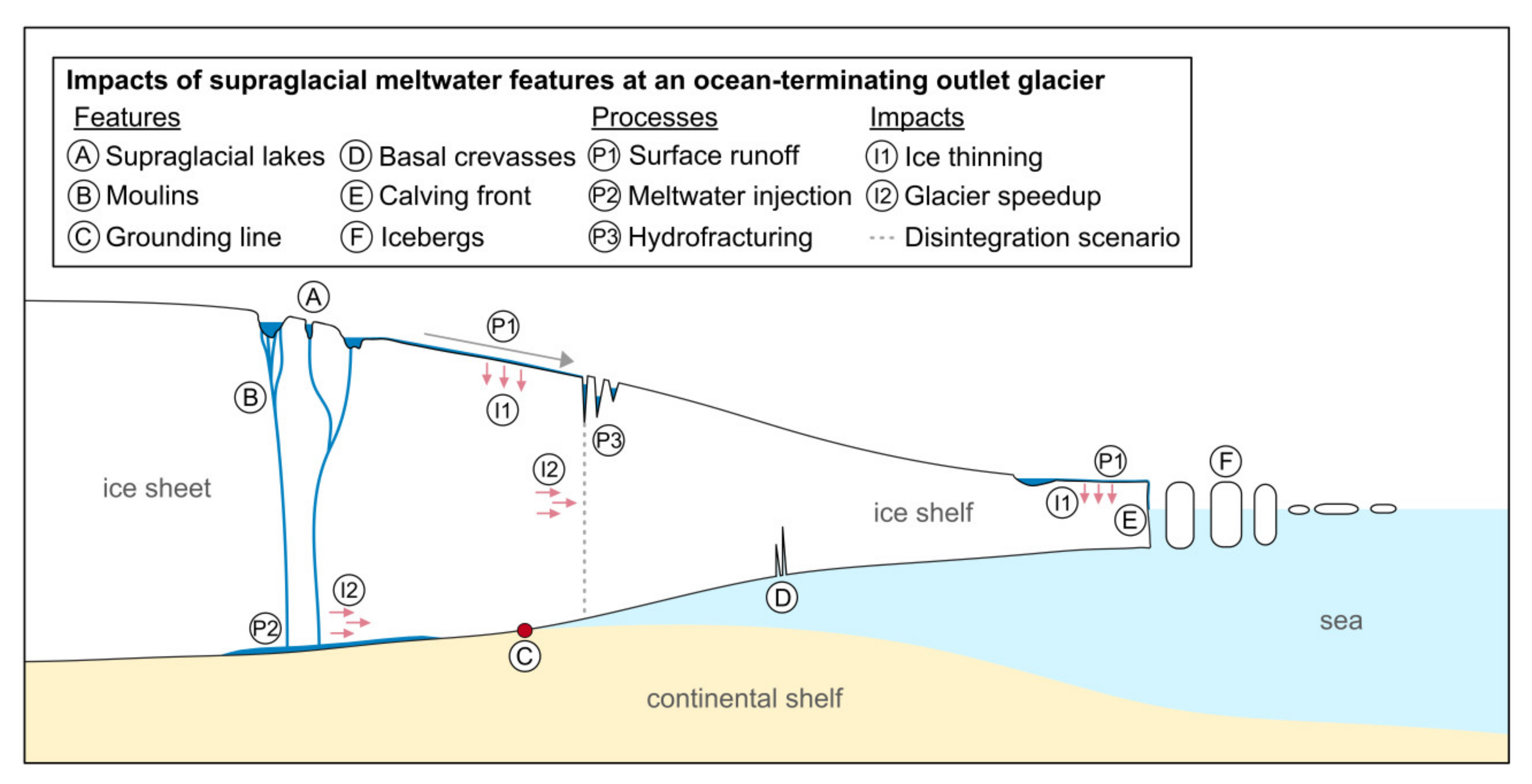
Holding ~91% of the global ice mass, the Antarctic Ice Sheet (AIS) is the biggest potential contributor to global sea-level-rise [1]. With accelerating global climate change [2], it is of essential need to understand the response of the AIS to further increasing ocean or surface air temperatures and to evaluate its potential contribution to future sea-level-rise. Increased surface air temperatures may directly impact the AIS through enhanced surface melting resulting in the formation of supraglacial lakes in local surface depressions above an impermeable snow/ice layer of the ice sheet [3]. In turn, the accumulation of supraglacial melt may affect Antarctic ice dynamics and mass balance through three main processes (see processes P1–P3 in Figure 1) [4]. First, increased surface melting and runoff (P1, Figure 1) may lead to enhanced ice thinning (I1, Figure 1) which directly contributes to a potentially negative Antarctic Surface Mass Balance (SMB) [4]. Second, the temporary injection of meltwater to the bed of a grounded glacier (P2, Figure 1) may enhance basal sliding and cause transient ice flow accelerations and increased ice discharge (I2, Figure 1), as observed over the Greenland Ice Sheet (GrIS) [5,6,7,8,9] and only recently along the Antarctic Peninsula (API) where drainage events triggered rapid ice flow accelerations with velocities up to 100% greater than the annual mean [10]. The third mechanism involves a process called hydrofracturing, i.e., meltwater-induced ice shelf collapse (P3, Figure 1). Here, the rapid drainage of surface lakes into fractures and crevasses of an ice shelf, for example formed through repeated filling and draining of lakes, initiates their downward propagation and the consequent calving of large icebergs or removal of entire ice shelves [4,11]. With the loss of the efficient buttressing force of an ice shelf, the inland ice accelerates and ice discharge increases (I2, Figure 1), as observed after the collapses of several API ice shelves such as Larsen B [12,13,14,15,16,17]. In addition, the enhanced presence of supraglacial melt decreases the surface albedo of ice while increasing the absorption of incoming solar radiation, which initiates a positive feedback that further triggers surface melting [18,19]. With enhanced surface melting, the number of exposed rock similarly increases which again accelerates ice melting through a decreasing albedo [20,21]. Figure 1 shows supraglacial lakes on an Antarctic ocean-terminating outlet glacier, where the impact of supraglacial meltwater on ice dynamics is illustrated schematically.
In order to investigate the impact of supraglacial meltwater accumulation on Antarctic ice dynamics and mass balance in more detail, a comprehensive mapping of Antarctic supraglacial lakes is required. While ground-based surveys of the AIS are time-consuming and limited in spatial extent, spaceborne remote sensing provides a means of mapping supraglacial lakes at unprecedented spatial coverage and detail. To date, most knowledge about supraglacial lakes results from studies on the GrIS, where ice mass loss is dominated by surface melting [4,22]. Yet, only few studies employed remote sensing data to investigate the characteristics and distribution of supraglacial lakes in Antarctica. Remote sensing based mapping approaches developed for supraglacial lake detection on the GrIS include several semiautomated techniques (e.g., [23,24,25,26]) as well as partly automated approaches using optical Moderate-Resolution Imaging Spectroradiometer (MODIS) images at low spatial resolution [27,28,29,30,31], yet they are found to be far less accurate than manual delineation techniques [32]. On the other hand, Antarctic studies of surface melt accumulation using remote sensing data mostly rely on manual to semiautomated mapping techniques including the solely visual identification of melt features (e.g., [33,34]) or Normalized Difference Water Index (NDWI)-based thresholding techniques (e.g., [20,35]) usually requiring manual postprocessing or an adaptation of thresholds when dealing with large-scale analyses and image time-series [20]. Regarding the geospatial distribution of supraglacial lake studies in Antarctica, most research focused on regions along the API [10,15,36,37], on selected glacier basins in East Antarctica [33,34,35,38,39] as well as on larger scale investigations of which two had their focus on East Antarctica [20,40] and one on selected basins across the AIS [21]. Starting with studies focusing on the API, Tuckett et al. [10] used Landsat 4, 5, 7 and 8 as well as Sentinel-2 imagery to manually identify melt and to link it to accelerated ice flow on several API glaciers. Next, Munneke et al. [36] used Sentinel-1 images to manually identify surface melt near the grounding line of Larsen C Ice Shelf and Glasser and Scambos [15] and Leeson et al. [37] used optical and radar imagery to manually map surface ponds on the Larsen B Ice Shelf prior to its collapse. Studies with focus on glacier basins in East Antarctica include the analysis of Langley et al. [33] who manually digitized supraglacial lakes from Advanced Spaceborne Thermal Emission and Reflection Radiometer (ASTER) and Landsat 7 images at Langhovde Glacier. Moreover, Fricker et al. [38] manually identified supraglacial lakes in ICESat (Ice, Cloud and Land Elevation Satellite) elevation tracks over Amery Ice Shelf and Bell et al. [35] detected supraglacial lakes in Landsat 8 imagery covering Nansen Ice Shelf applying Normalized Difference Water Index (NDWI) thresholding. Supraglacial lakes have also been observed in Landsat images along Wilkes Land [39] and in MODIS and Landsat 7 images across Nivlisen Ice Shelf [34]. Larger scale investigations were conducted after it was revealed that Antarctic surface melting is more widespread than previously assumed. To start with, a recent study for the first time identified ~700 surface drainage systems in Landsat, ASTER and WorldView satellite images across Antarctica [21]. Another study used a semiautomatic NDWI thresholding method on Sentinel-2 and Landsat 8 data to map the 2017 distribution of supraglacial lakes in East Antarctica [20]. The authors in [40], on the other hand, propose a threshold-based method based on Sentinel-2 and Landsat 8 data to be implemented for Antarctic-wide supraglacial lake detection in the future. In their study, specific focus is on sections of the Roi Baudouin, Nivlisen, Riiser-Larsen and Amery Ice Shelf in East Antarctica, where lake extents and volumes were tracked for several time steps. Even though the recent study by Moussavi et al. [40] was the first to propose an automated lake detection method for Antarctica, it still has to be implemented and tested on a larger scale beyond the test regions analyzed for East Antarctica.
Despite the shown potential of Earth Observation for detecting and mapping supraglacial lakes on the AIS, data of the Sentinel-2 mission offer new opportunities for automated mapping of supraglacial lakes at unprecedented spatial resolution (10 m) and coverage. The Sentinel-2 constellation consists of two optical satellites, Sentinel-2A and Sentinel-2B, enabling the monitoring of polar regions with up to daily revisit times. Both Sentinel-2A and Sentinel-2B carry a passive Multispectral Instrument (MSI) recording the sunlight reflected from the Earth’s surface in 13 spectral bands. To date, Sentinel-2 data have been underexploited and no time-efficient mapping method has been implemented for a systematic and automated mapping of Antarctic supraglacial lakes. In fact, a circum-Antarctic record of supraglacial lakes with full ice sheet coverage is entirely missing. This is not only required to evaluate the spatial distribution of meltwater features but also to quantify their water volume, their temporal dynamics or to obtain an input dataset for SMB as well as overall mass balance calculations [41,42]. In addition, it is of fundamental importance to better understand the role of supraglacial meltwater on ice shelf stability as ~75% of Antarctica’s coastline is fringed by floating ice shelves [43] providing important buttressing to the grounded inland ice [44,45]. Given that Antarctic surface melting is projected to double by 2050 [46], supraglacial lakes will be even more prevalent in the future and most likely spread farther inland, which again highlights the need for an automated mapping method using high spatial resolution satellite data. Besides, the Antarctic surface and basal hydrological systems could further connect and surface melting could become a major contributor to accelerated ice mass loss from the AIS [4].
In this context, the objective of this study was to develop an automated method for Antarctic supraglacial lake mapping using state-of-the-art image processing techniques. More precisely, we employed a supervised Machine Learning (ML) algorithm, namely Random Forest (RF), trained on optical Sentinel-2 and auxiliary TanDEM-X topographic data. The main focus during method development was to ensure its spatio-temporal transferability. In the following, we first present the corresponding study sites and datasets selected for model training and testing as well as all necessary preprocessing steps (Section 2.1 and Section 2.2). Following this, Section 2.3 and Section 2.4 present our research method including RF model training and parameter optimization, postclassification as well as the methods used for validating the model. In Section 3, we present the lake extent mapping results as well as all the outcome of the accuracy assessment and Section 4 discusses the classification results and accuracies as well as remaining limitations of our supraglacial lake detection algorithm. Finally, Section 5 summarizes the findings of this paper. At this point, it has to be noted that the automated mapping results of this study will be used as input for the development of a Sentinel-1 based supraglacial lake detection method, to be presented in a subsequent study.
2. Data and Methods
The whole workflow for automated supraglacial lake mapping is shown in Figure 2. Accordingly, it can be divided into (1) data preparation, (2) image classification, (3) postclassification and (4) accuracy assessment. Unless indicated otherwise, all processing was done using the Python programming language. Before providing a more detailed insight into the applied datasets and methods, the following section summarizes the study sites selected for model training and testing.
2.1. Selection of Study Sites
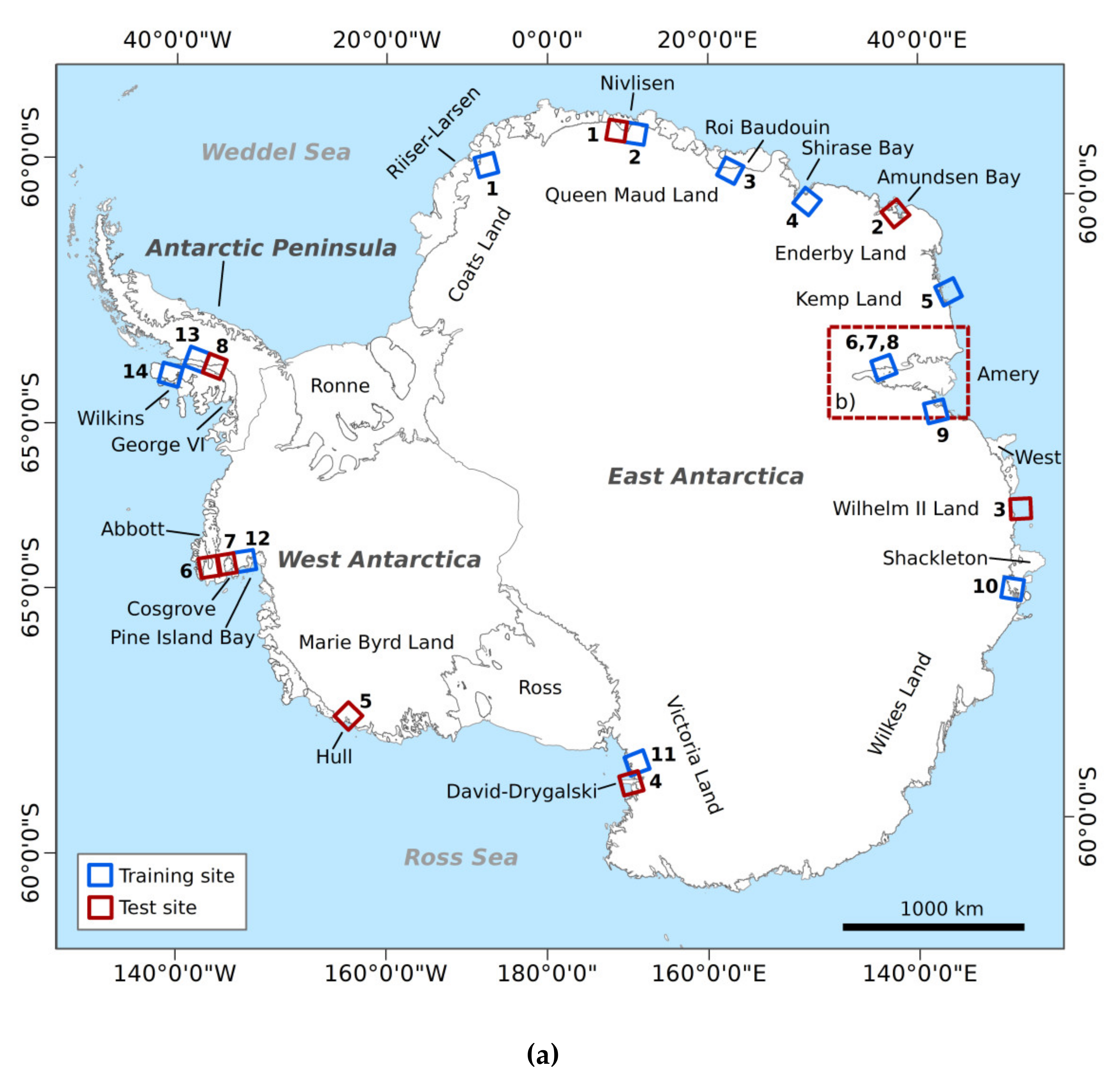
The selection of study sites was based on known supraglacial lake locations (e.g., [20,21,34,47,48,49]) as well as the visual inspection of satellite imagery on Google Earth Engine. To ensure the spatial transferability of our supraglacial lake detection algorithm, we selected training and test regions evenly distributed across Antarctica containing information on all different types of environments and surface conditions. These include blue ice, wet or slushy snow in lower elevations, dry snow in higher elevations, deep and shallow supraglacial lakes as well as regions that are heavily crevassed or spotted with rock outcrop. For temporal transferability, we additionally restricted our study site selection primarily to occurrence of supraglacial lakes during the summer melt seasons of year 2019 for training regions and years 2017 and 2018 for test regions. This resulted in 14 training regions and eight spatially independent test regions (see Figure 3a, Table 1). Of the training areas, 11 were located on the East Antarctic Ice Sheet (EAIS), representing the largest of all three Antarctic regions, one was on the West Antarctic Ice Sheet (WAIS) and two covered regions on the API. Of the test sites, four were located on the EAIS, three on the WAIS and one on the API.
Furthermore, our full classification workflow was tested for large-scale application over Amery Ice Shelf (Figure 3b), where meltwater accumulation is particularly prevalent and where the largest of all currently known Antarctic supraglacial lakes is located [20,21]. This site was selected to show the potential of our method for analyzing spatio-temporal supraglacial lake dynamics. Figure 3a shows an overview map of Antarctica as well as the spatial locations of all training and test sites. An enlargement of the additional test region over Amery Ice Shelf is illustrated in Figure 3b.
2.2. Input Data
For the identified training and test sites, corresponding input data were selected. In this study, mainly optical Sentinel-2 (Section 2.2.1) and TanDEM-X Digital Elevation Model (DEM) (Section 2.2.2) data were used. Additionally, we manually created class labels to support model training (Section 2.2.3). Here, only the surface classes “water”, “snow/ice”, “rock” and “shadow” were considered. A further categorization, e.g., according to varying lake depths, different rock or snow/ice types ranging from wet over slushy to dry snow was not performed as the main aim of the present study was to discriminate between water and nonwater.
2.2.1. Sentinel-2
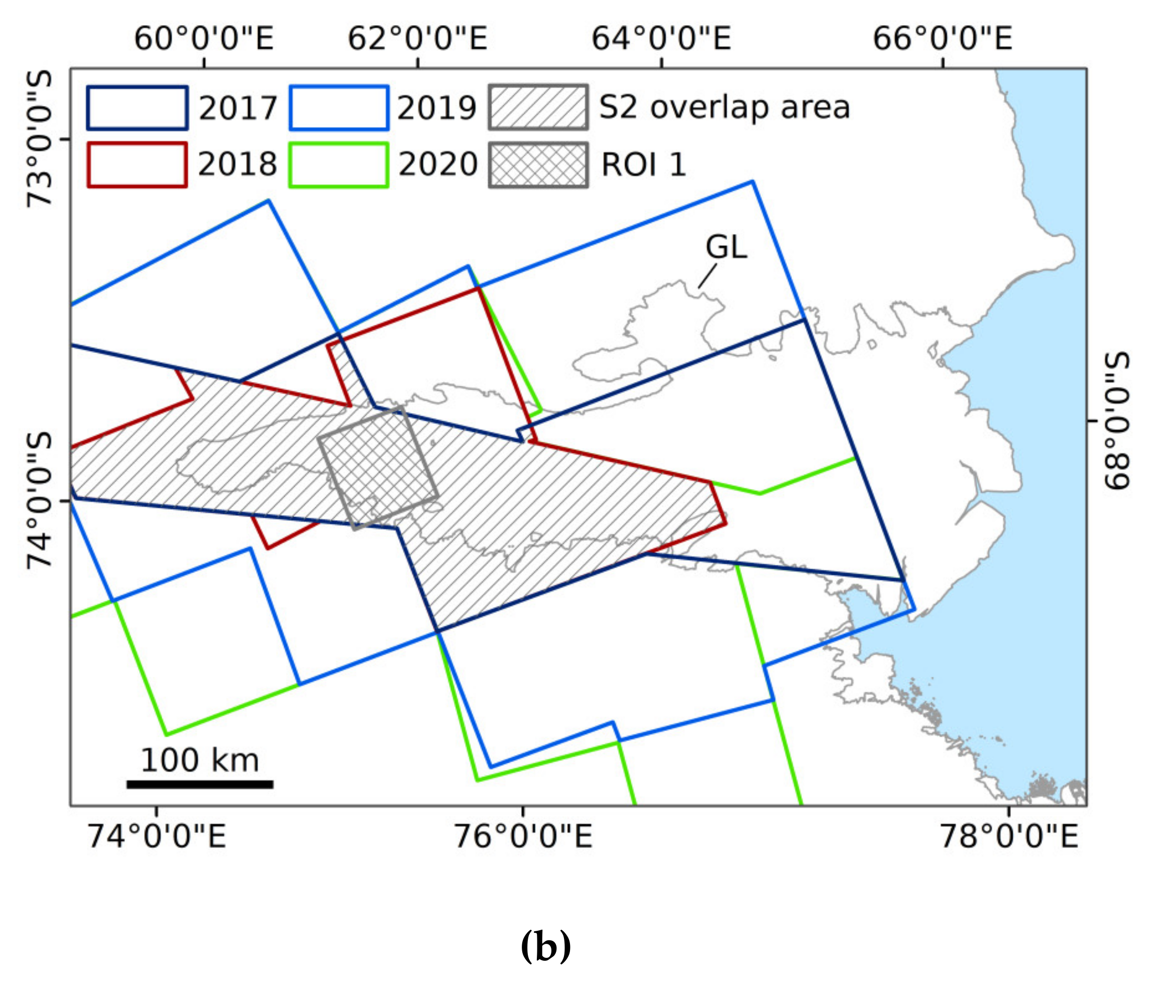
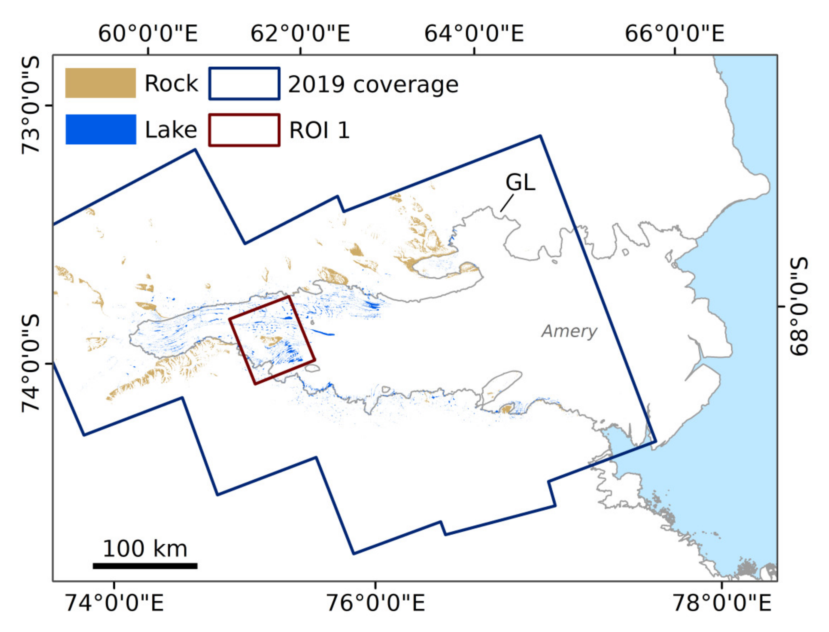
As visible in Table 1, each training and test region corresponds to one Sentinel-2 granule. In detail, the selection of Sentinel-2 imagery was based on the following criteria. First of all, we only considered imagery with cloud coverage less than 10% and acquired at sun elevation angles larger than 20° (see [40]). Second, to ensure the temporal transferability of our algorithm also during one individual melt season, the 14 Sentinel-2 training granules were chosen to include dates between early and late January 2019 (Table 1). On the other hand, to evaluate the temporal transferability of our algorithm, the eight test granules were selected to cover dates during the melt seasons of 2017 and 2018 (Table 1). Accordingly, 84 additional Sentinel-2 acquisitions were selected for employing our workflow for large-scale application over Amery Ice Shelf (Table S1), where we calculated maximum lake extents for four consecutive melt seasons (2017, 2018, 2019, 2020). As Level-2A Bottom-Of-Atmosphere (BOA) data over Antarctica are only provided since December 2018 [51], all Level-1C Top-Of-Atmosphere (TOA) data of 2017 and 2018 were corrected for atmospheric effects using Sen2Cor, a processor for retrieval of surface reflectance developed specifically for Sentinel-2 [52,53]. Table 1 lists the Sentinel-2 acquisitions selected for model training and testing and Table S1 the acquisitions covering Amery Ice Shelf. On the other hand, Figure 3b illustrates the coverage of Sentinel-2 granules for all regarded melt seasons over Amery Ice Shelf as well as their areal overlap and ROI 1, selected for quantitative analysis in Section 3.2.2.
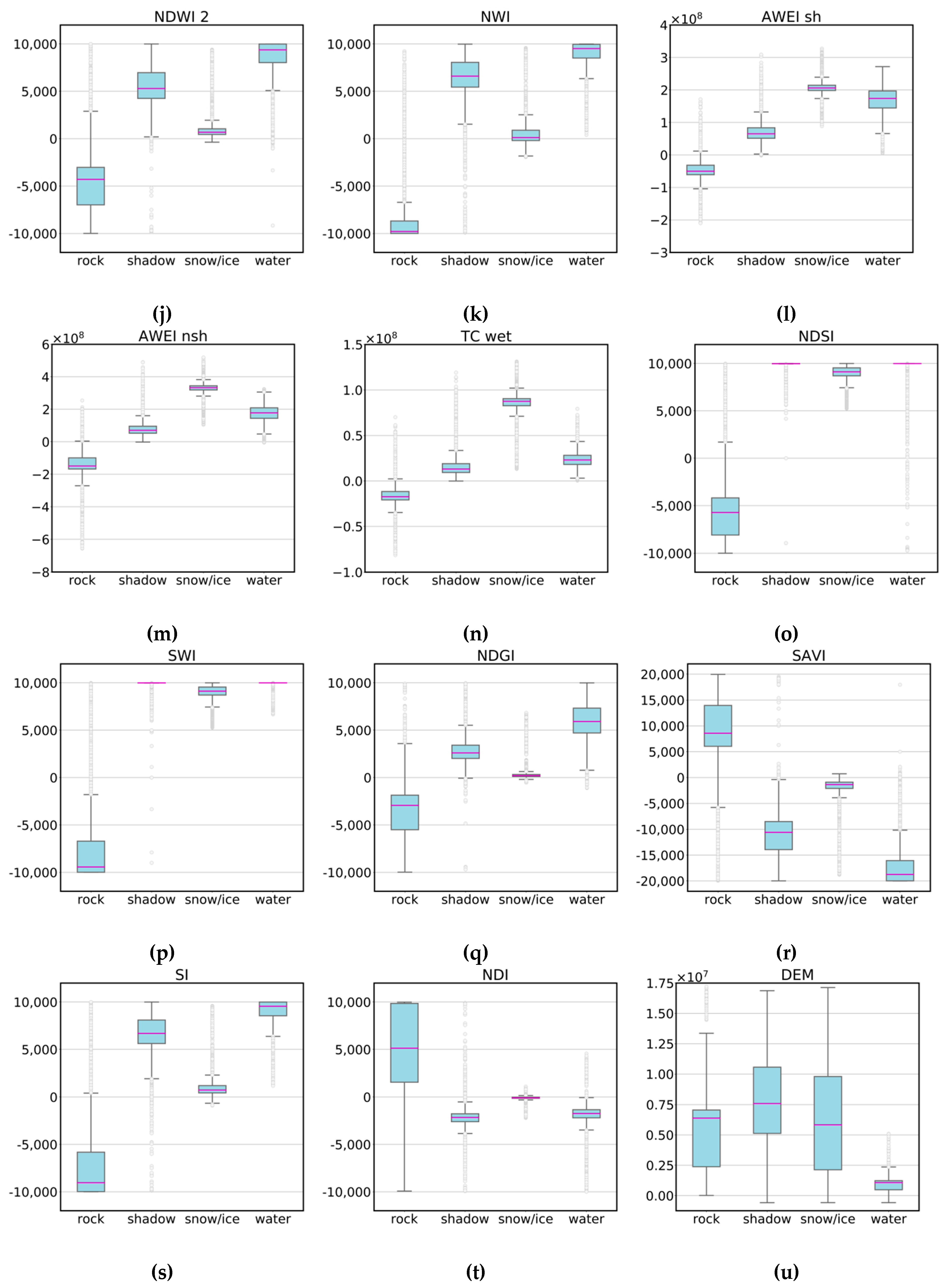
Following a discrimination analysis of the reflectance properties of water, snow/ice, rock and shadow on ice (Figure 4), only Sentinel-2 bands 2-8A were included for classification (Table 2). In addition, the selected Sentinel-2 bands as well as bands 11–12 were used to derive spectral indices to be fed to the classifier. In this study, we calculated 12 different indices for each granule out of which 11 were collocated from external reference studies and one was formulated as part of this study. First, the NDWI indices (NDWI1, NDWI2) [30,54,55], the New Water Index (NWI) [56], the Tasseled Cap for wetness (TCwet) [57,58] and the Automated Water Extraction Index with the option of shadow (AWEIsh) or dark area removal (AWEInsh) [59] (Figure 4i–n) were derived to support the classification of open surface water. Second, the modified Soil-Adjusted Vegetation Index (SAVImod) [60], the Soil/Water Index (SWI), the Modified NDWI (MNDWI) (or Normalized Difference Snow Index (NDSI)) [61,62], as included in the European Space Agency’s (ESA) Cloud/Snow Detection Algorithm [63] and the Normalized Difference Glacier Index (NDGI) [64] were included as training variables in order to support the identification of mainly rock and ice (Figure 4o–r). Third, the NWI, the SAVI, the AWEIsh as well as an additional modified Shadow Index (SImod) [65] (Figure 4k,l,r,s) were included for a better differentiation between shadow on ice and water, having almost identical reflectance properties in most of the bands/indices (Figure 4). Finally, the Normalized Difference Index (NDI) (Figure 4t) was formulated as part of this study and was added with the intention of providing further spectral information supporting the discrimination between all classes. Table 3 lists all derived indices as well as their mathematical formulations.
2.2.2. TanDEM-X DEM
To support classification, we included an edited version of the 90-m Antarctic TanDEM-X DEM in our workflow. The underlying SAR data of the Antarctic DEM were acquired between April 2013 and November 2014 and cover the full Antarctic continent. In addition, we derived topographical parameters including slope, roughness and relief to be included as training variables (Figure 4u–x). The slope layer was also used for postclassification (Section 2.3.2). Moreover, we used the elevation data to conduct topographical analyses of supraglacial lake occurrence on Amery Ice Shelf.
2.2.3. Training Labels
Training labels are required to support ML classification algorithms during model training. As no circum-Antarctic supraglacial lake inventory exists to date, training labels were created manually in Google Earth Engine based on the Sentinel-2 training granules listed in Table 1. In agreement with Figure 4, we drew and labeled polygons for four main classes, namely “water”, “snow/ice”, “rock” and “shadow”. Here, care had to be taken in selecting training samples as homogeneous as possible in order to ensure a sufficient quality of the training dataset. For model training, the manually created polygons were rasterized.
2.2.4. Data Harmonization
Concluding data preparation, we harmonized all input data to the highest spatial resolution of Sentinel-2 (10 m) using the nearest neighbor algorithm. Additionally, all data were reprojected to the coordinate reference system of the corresponding Sentinel-2 granules. In this context, all 14 training datasets consisting of Sentinel-2 and TanDEM-X variables were clipped using the rasterized training labels. In a final step, we collocated all extracted datasets to a single large training dataset which was then used to train and calibrate the classification model. Conversely, the eight independent test datasets consisted of the described Sentinel-2 and TanDEM-X variables only.
2.3. Image Classification
2.3.1. Random Forest Classifier
Random Forest (RF) is an easy-to-implement supervised ML classifier and has frequently been applied for remote sensing classification problems, e.g., to classify wet and dry snow in Sentinel-1 SAR data [66], for wetland mapping using high-resolution multispectral imagery [67], for rice crop classification using Sentinel-1 data [68] or for tree species classification using WorldView-2 data [69], to only name a few. In this study, RF was chosen due to its various advantages compared to other ML classifiers including the comparatively low computation time, the simple parameter tuning and low risk of overfitting and its parallel processing capabilities [70,71,72,73].
RF is characterized by an ensemble of uncorrelated decision trees. In detail, the algorithm behind RF is based upon bootstrap aggregating, or bagging, meaning that each individual decision tree is built on the basis of a randomly sampled subset of training data [70,71,72]. Specifically, the randomly sampled subset represents about two thirds of the original training data and the remaining third, also referred to as Out-Of-Bag (OOB) samples, is used for internal cross-validation [70]. To find the best split at each node of a decision tree, RF uses a metric called Gini Impurity [70]. In this context, Gini Impurity is utilized to calculate the mean decrease in Gini returning the importance of employed variables during classification [70]. For new unclassified data, each sample is predicted based upon the maximum votes of all independent decision trees [70,71].
For implementation of RF, we used Python’s skicit-learn library [74]. In particular, RF was trained on a subset of 70% of the training data and tested on the remaining 30%. To optimize the default RF parameter selection including the number of trees in the forest, the maximum depth of a tree, the minimum number of samples required to split an internal node or the minimum number of samples required at a leaf node, we used scikit-learn’s “RandomizedSearchCV” and “GridSearchCV” functionalities [74,75]. Additionally, to return the importance of all input variables used for model training, the mean decrease in Gini was calculated.
2.3.2. Postclassification
Postclassification was necessary to (1) obtain a surface water classification map only and (2) remove misclassified lake pixels from the automatically returned RF classification map. Therefore, a first step of the postclassification involved the masking of the shadow, rock and ice classes in the RF classification result itself. Within the same step, it was possible to extract a rock classification map as side-product (e.g., Figure 10) which was further refined by additional band thresholding. Second, as few outliers were still present in the preliminary surface water classification map, we implemented a range of automated postclassification steps, valid for all independent test data. With more detail, we created an accumulated mask resulting from the following conditions and thresholds (see Figure 2).
At first, regions with slope values greater than 5% were defined to be excluded. This step allowed eliminating most errors due to the misclassification of topographic shadow on ice as open surface water, knowing that surface water cannot accumulate in such steep terrain. In contrast to Figure 4v suggesting the use of an even lower slope threshold for the water class, this value was set conservatively due to the TanDEM-X DEM being from a different time step and its considerably lower spatial resolution compared to Sentinel-2. In fact, we found that lower slope thresholds oftentimes cause the masking of true positive lake pixels, e.g. where steep crevasses or ice fractures used to be present during acquisition of the underlying DEM data. In a subsequent step, the Scene Classification Layer (SCL), provided alongside the Sentinel-2 band layers, was used to exclude pixels in classes 1, 2 and 3 representing saturated or defective pixels, dark area pixels and cloud shadow respectively. For both the slope and SCL masks, we introduced a binary dilation of two pixels around each masked pixel. In order to eliminate false lake pixels over open ocean, and particularly around or atop calved icebergs, another step involved the masking of all pixels seaward of a MODIS coastline product of the National Aeronautics and Space Administration (NASA) Making Earth System Data Records for Use in Research Environments (MEaSUREs) program [76,77]. In particular, the MODIS coastline dataset was derived from the Mosaic of Antarctica (MOA) surface morphology map, a data product generated on the basis of 416 MODIS Aqua/Terra image swaths acquired during the 2013/2014 austral summer season [76,78]. Next, as shadow on ice in very deep crevasses as well as below thick clouds was in few cases still misclassified as water, we set additional threshold values for Sentinel-2 band 2 as well as the NWI, NDWI2, NDGI, SAVI and SI layers analyzing the reflectance properties in Figure 4. At this point it has to be noted that common cloud masking algorithms such as FMask [79] do not deliver satisfactory results over Antarctica.
Following the fusion of all masks, we applied it to the generated RF classification product. Furthermore, we eliminated lake areas smaller than three pixels (or 300 m2) using a morphological erosion filter. Accordingly, we eroded areas smaller than three pixels present as “no-lake” pixels within the lake boundaries. In summary, the final Sentinel-2 classification product discriminated between classes “water” and “nonwater” only and was provided at 10 m pixel resolution (Figure 2).
2.4. Accuracy Assessment
As no freely available circum-Antarctic lake inventory exists to date, an accuracy assessment was performed using randomly created point samples covering the extent of the classification maps. To ensure an adequate point sampling rate in areas directly surrounding water pixels potentially prone to misclassification, we introduced a buffer of 250 m around every water pixel within a classified test scene. Following this, we used ArcMap’s “Create Accuracy Assessment Points” functionality to randomly sample 2000 data points within both the buffered water and the surrounding nonwater class (Figure S1). For validation, Sentinel-2 imagery was used as ground truth.
The results of the point comparisons were evaluated by means of a confusion matrix visualizing the performance of our workflow for both the “water” and the “nonwater” class. In detail, the creation of a confusion matrix allowed deriving common statistical accuracy metrics including Recall and Precision, F-score, errors of commission and omission as well as Cohen’s Kappa [80,81]. To start with, the Recall (R), oftentimes referred to as Producer’s Accuracy, was computed dividing the number of true positives within a class prediction by the total number of true class samples. Next, the Precision (P) (or User’s Accuracy) was calculated dividing the number of true positive pixels by the total number of predicted pixels of a class [80,81]. In order to include a measure capturing the Recall and Precision conjointly, the F-measure (F1) was computed to provide their harmonic mean [80,81].
For completeness, we calculated the Errors of Omission (EO) and the Errors of Commission (EC), also referred to as False Negative Rate (FNR) and False Positive Rate (FPR) respectively. While the EO returns the number of False Negatives (FN) with respect to all true class samples, the EC describes the rate of all False Positives (FP) with respect to all predicted samples of a class. All metrics were calculated for each class individually as the calculation of average values would not be representative at class-level. As an overall accuracy measure, we additionally computed Cohen’s Kappa (K) using the following formula [82,83]:
where the Overall Accuracy (OA) is calculated dividing the sum of all True Positives (TP) and True Negatives (TN) of the classification result by the total number of sampled points (TS) and the Expected Accuracy (EA) is calculated from TP, TN, FP, FN and TS:
According to this, K measures the similarity between classification and ground truth taking into account the expected accuracy of a random classifier, where higher values of K, measured between 0 and 1, represent better agreement than lower values [83].
3. Results
3.1. Importance of Variables
Figure 5 shows the variable importance of all input features averaged for all training regions and classes. As can be seen, particularly the Sentinel-2 bands as well as a range of spectral indices including TCwet, AWEInsh, AWEIsh and SWI were considered informative for overall image classification. On the other hand, the topographic variables including DEM, slope, roughness and relief returned feature importances <3.
3.2. Lake Extent Mapping
3.2.1. Test Regions
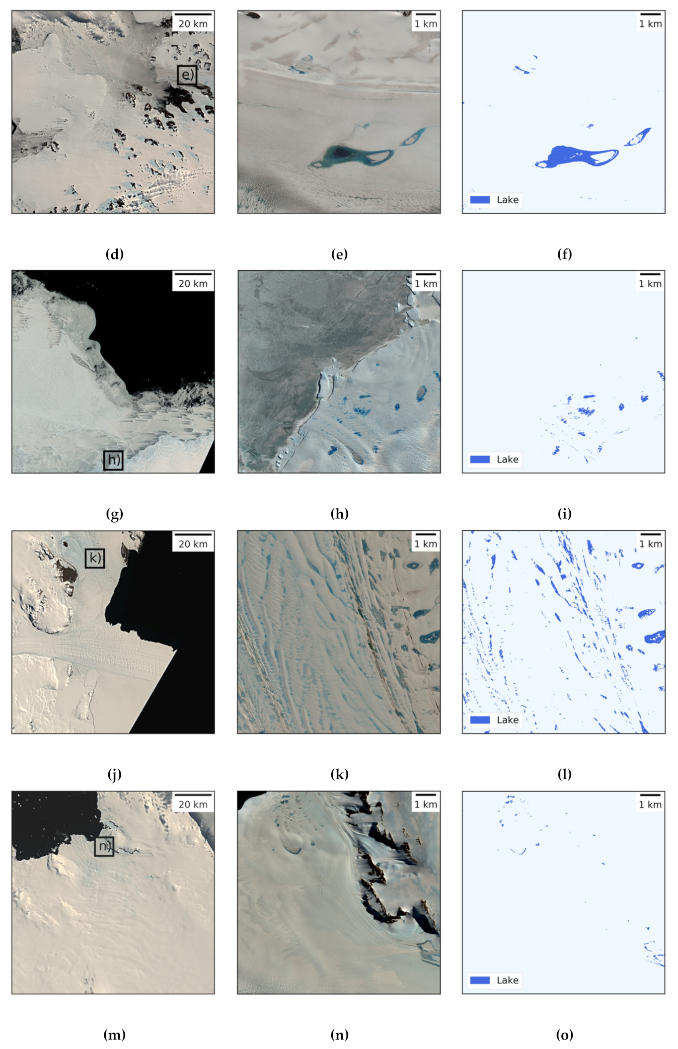
Figure 6 illustrates the Sentinel-2 test scenes alongside smaller image extracts as well as their corresponding classification maps. In all eight test regions, numerous supraglacial meltwater features were detected (Figure 6c,f,i,l,o,r,u,x) and ranged from smaller elongated surface ponds, e.g., over George VI (Figure 6x) and Nansen Ice Shelf (Figure 6l), to larger meltwater lakes partly frozen over on their surface, as found for Nivlisen Ice Shelf (Figure 6c) and in Amundsen Bay in East Antarctica (Figure 6f). Of all test scenes (see Table 1), Nivlisen Ice Shelf returned by far the largest supraglacial lake extent (28.96 km2), closely followed by George VI Ice Shelf (28.1 km2), Drygalski Ice Tongue (24.52 km2) and Amundsen Bay (12.64 km2) (Table 4). For all other test scenes, meltwater features covered an area <5 km2 (Table 4).
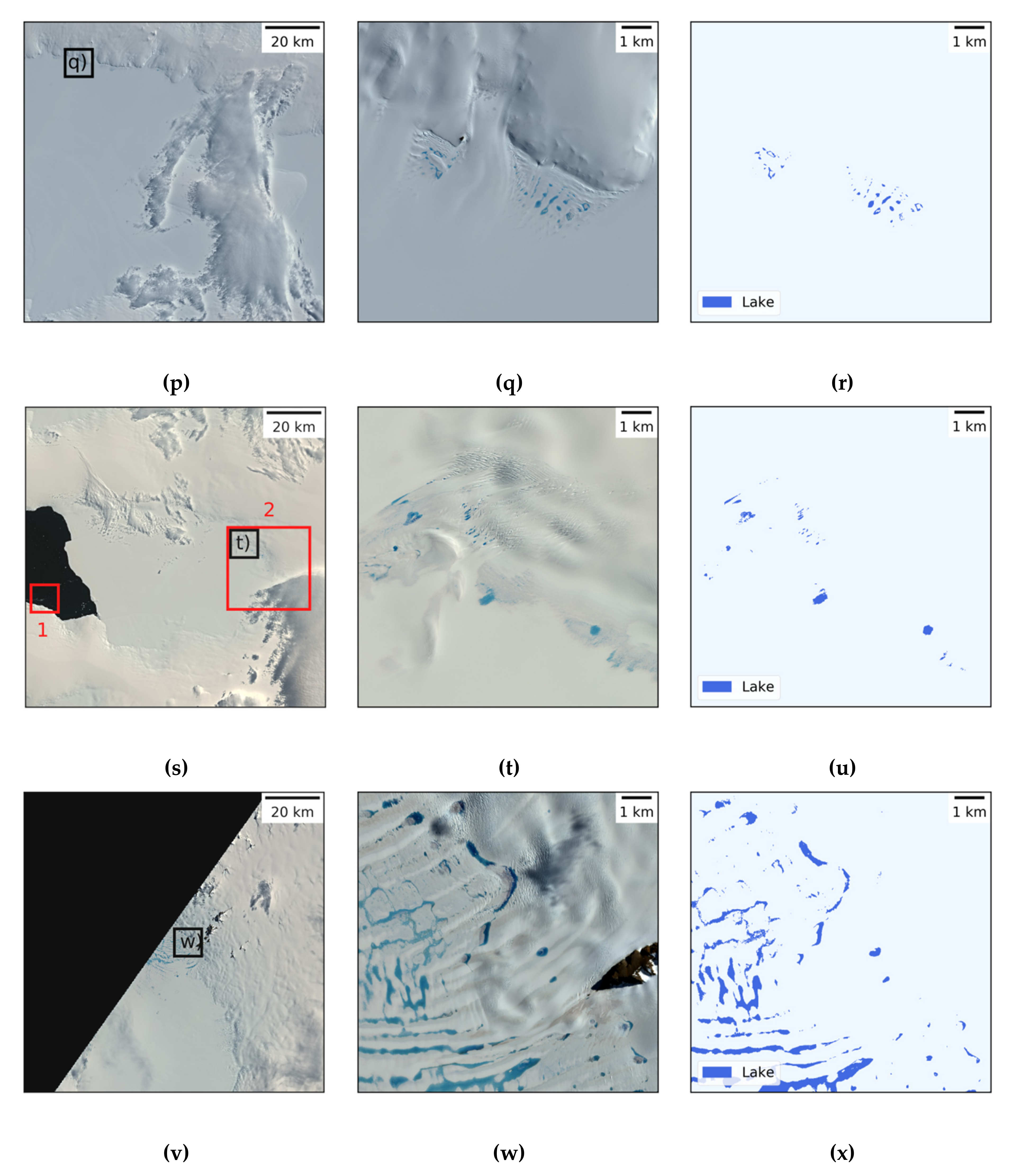
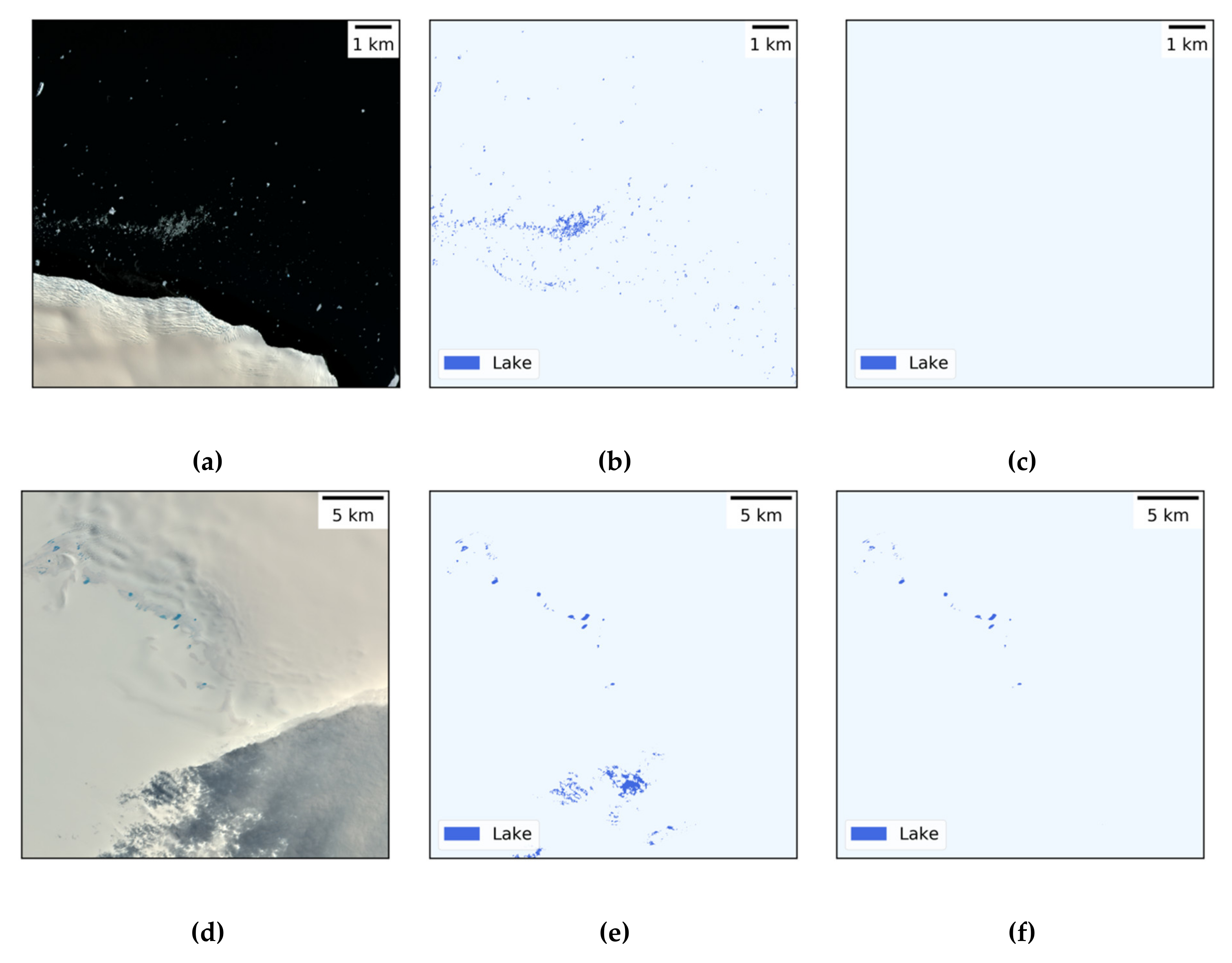
To show the performance of our automated workflow for test scenes containing cloud shadow and open ocean usually requiring the manual removal of misclassified lake pixels with traditional methods (e.g., [20]), Figure 7a,d illustrate exemplary Sentinel-2 extracts for regions 1 and 2 over Cosgrove Ice Shelf (see Figure 6s) as well as the corresponding classification maps before coastline and bands and indices masking (Figure 7b,e) as well as after these postclassification steps (Figure 7c,f). As can be seen, the initial classification maps before masking (Figure 7b,e) still contained outliers over the open ocean (Figure 7b) or due to shadow on ice below thick clouds being misclassified as surface water (Figure 7e). After postclassification, these artifacts were mostly removed and open ocean as well as cloud shadows on ice were successfully discriminated from supraglacial meltwater (Figure 7c,f). Moreover, comparing the Sentinel-2 image extracts in Figure 6h,n,t,w to the classification maps in Figure 6i,o,u,x, it can be noted that rock and topographic shadow on ice (e.g., Figure 6o,x) as well shadow in crevasses (e.g., Figure 6i,u) were almost entirely masked applying our workflow. The same applies to different snow and ice types including blue ice (e.g., Figure 6i,o), polluted (e.g., Figure 6f) and even slightly slushy snow (e.g., Figure 6c).
3.2.2. Spatio-Temporal Lake Dynamics on Amery Ice Shelf
The classification maps over Amery Ice Shelf revealed highly varying supraglacial lake extents for all regarded melt seasons (Figure 8 and Figure 9). Considering the Sentinel-2 overlap area shown in Figure 3b, maximum lake extent was computed at ~699 km2, ~311 km2, ~763 km2 and ~337 km2 during the 2017, 2018, 2019 and 2020 melt seasons respectively (Figure 9). For ROI 1, a similar pattern was observed and the areal extent of supraglacial meltwater features was highest in 2017 and 2019 and lowest in 2018 and 2020 (Figure 8 and Figure 9).
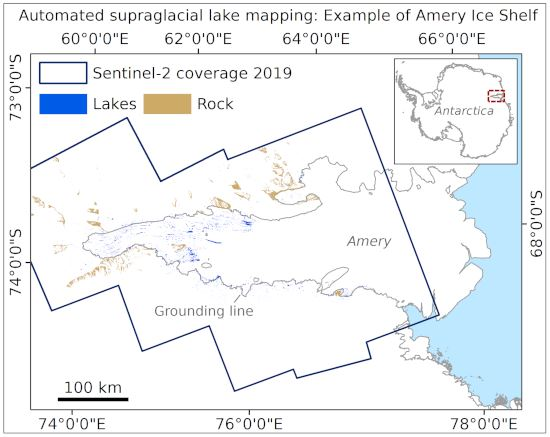
In all four years, surface meltwater was most abundant in the southern section of Amery Ice Shelf as well as along the southern and eastern grounding line, also visible in the 2019 mapping result (Figure 10). In fact, almost three quarters of all supraglacial lake pixels in 2018 and 2020 as well as around half of all lake pixels in 2017 and 2019 were detected within 10 km of the grounding line, downloaded from the SCAR ADD [50]. Moreover, >70% of all lake pixels in 2017, 2018, 2019 and 2020 were found on the floating ice shelf downstream of the grounding line (Table 5). At the same time, between ~ 52% and ~ 67% of all supraglacial lake pixels in 2017, 2018, 2019 and 2020 were ≥300 km inland of the MOA coastline (Table 5). Overall, the largest supraglacial lake formed slightly to the north of ROI 1 (see Figure 10) and reached its maximum size (~66 km2) during the 2017 melt season.
Considering the elevation range of supraglacial lake occurrence, the lake located in the highest altitude was detected at 1615 m in 2020 and the lake located in the lowest altitude was found at 16 m in 2019. On the other hand, the mean elevation of supraglacial lake occurrence was highest in 2017 (177 m) and 2019 (156 m) and lowest in 2018 (139 m) and 2020 (132 m). Finally, investigating the distance of supraglacial meltwater to rock, ≤35% of all lake pixels in 2017 and 2019 and ≥56% of all lake pixels in 2018 and 2020 were within a buffer zone of 5 km around rock outcrop (Table 5). In years with overall low surface melt accumulation (2018, 2020), supraglacial lakes thus formed at lower mean elevations and closer to the grounding line as well as to rock outcrop while revealing a more widespread distribution across the whole ice shelf and in higher mean elevations in years with increased lake occurrences (2017, 2019).
3.3. Accuracy Assessment
Table 6 lists the computed accuracy and error rates for all Sentinel-2 test regions. To start with, the average rate of false negatives (EO) of the water class was computed at 17.25% and the average EO of the nonwater class was measured at 0.22%. For the water class, the EO ranged from 3.91% over George VI Ice Shelf to 30.99% and 35.29% over Abbott Ice Shelf and Hull Glacier respectively. On the other hand, the EO of the nonwater class ranged between 0% (e.g., Abbott Ice Shelf) and 0.88% (Nivlisen Ice Shelf). Similarly, the average rate of false positives (EC) was higher for the water class (9.24%) than for the nonwater class (0.45%). Within the water class, the EC ranged between 0% (e.g., Abbott Ice Shelf) and 50% (Hull Glacier) and between 0.27% (George VI Ice Shelf) and 1.13% (Abbott Ice Shelf) in the nonwater class. The recall and precision were analyzed conjointly in terms of the F1 score, which revealed average values of 86.05% and 99.66% for the water and the nonwater class respectively. For the water class, F1 was lowest for the test scenes over Hull Glacier (56.41%) and Abbott Ice Shelf (81.67%) and highest for the scenes covering George VI (98.01%) and Cosgrove Ice Shelves (94.49%). On the other hand, the F1 score of the nonwater class ranged between 99.39% (Nivlisen Ice Shelf) and 99.87% (George VI Ice Shelf). Finally, the computation of K returned an average value of 0.857 for all test scenes while being lowest for Hull Glacier (0.560) and highest for George VI Ice Shelf (0.979).
4. Discussion
4.1. Importance of Variables
The variable importance plot in Figure 5 revealed the average importance of features collocated for all four classes within the training regions. Even though the number of variables used in this study was comparatively large where some variables returned lower importances than others, we decided not to reduce the number of input variables during model training. First of all, Figure 5 presents the importances for all four classes conjointly. Therefore, none of the bands or indices should be considered nonrelevant as they might still be important for at least one of the classes. Second, the selection of input variables was based upon a thorough literature research and spectral discrimination analysis (see Figure 4) confirming their suitability for the mapping of water, rock, snow/ice and shadow on ice. Third, as the main aim of this study was to develop a mapping approach transferable in space and time, a broader range of input variables allows for more flexibility during classification of spatially independent regions. Finally, the results of the accuracy assessment (Section 3.3) have proven the functionality of our approach, making a restriction of input variables unnecessary.
4.2. Mapping Results
According to the classification results in Section 3.2, supraglacial lakes were widespread during the 2017 and 2018 melt seasons over the test regions (Figure 6) as well as in 2017–2020 over Amery Ice Shelf despite some variance from year to year (Figure 8, Figure 9 and Figure 10). In fact, our study for the first time reports on supraglacial lake occurrence on Hull, Abbott and Cosgrove Ice Shelves in West Antarctica as well as on Nivlisen, West and George VI Ice Shelves in 2018 and on Amery Ice Shelf in 2019 and 2020. For all other test regions, our mapping results are in good agreement with independent studies, similarly reporting on extensive supraglacial lake occurrence in Enderby and Victoria Land during the 2017 melt season [20] as well as on Amery Ice Shelf during the 2017 and 2018 melt seasons [20,40]. More specifically, Moussavi et al. [40] used Landsat 8 scenes during the 2017 and 2018 melt seasons over Amery Ice Shelf to determine lake extents of ~720 km2 and ~380 km2 using a threshold-based approach as well as of ~640 km2 and ~240 km2 using an unsupervised clustering approach. In this study, maximum lake extents amount to ~699 km2 and ~311 km2 for the Sentinel-2 overlap area in 2017 and 2018, being in between the two estimates and therefore in overall good agreement with Moussavi et al. [40]. Deviations between the estimates most likely result from a slightly different temporal and areal coverage as well as from different analysis methods and data sources.
Furthermore, the application of our workflow revealed spatial characteristics of supraglacial lake occurrence for Amery Ice Shelf. Comparing our results in Section 3.2.2 to 2017 estimates obtained for East Antarctica [20], we find good agreement overall. In particular, the average elevation of supraglacial lake occurrence during 2017 was ~177 m while the highest lake was found at 1615 m in 2020. Similarly, Stokes et al. [20] report on lakes typically developing at low elevations (~100 m) while existing at elevations >1500 m. Next, ~87% of all lake pixels in 2017 were detected on the floating ice shelf (Table 5). Likewise, Stokes et al. [20] highlight that more than 80% of the 2017 lake extent in East Antarctica was located downstream of the grounding line. Lastly, we found that ~24% of all supraglacial lakes in 2017 occurred within 5 km distance to rock outcrop (Table 5) being in good agreement with the estimate (~35%) for 10 km distance in Stokes et al. [20]. Even though the conditions on Amery Ice Shelf might be slightly different to entire East Antarctica, the overall good agreement of results demonstrates the applicability of our method for analyzing spatio-temporal lake dynamics.
4.3. Accuracy Assessment
As mentioned above, the overall computed statistical accuracy metrics (Table 6) reveal the good functionality and spatio-temporal transferability of our workflow. Nevertheless, some test regions returned lower overall accuracy scores for the water class than others. For instance, reduced accuracies were found for the test regions covering Wilhelm II Land, Hull Glacier, Abbott Ice Shelf and Amundsen Bay. In this context, Hull Glacier returned by far the lowest accuracy scores (Table 6). Analyzing the classification map over Hull Glacier in detail, we found that shadow below a cluster of particularly thick clouds in the respective acquisition (see Figure 6m) explains the high rate of false positive lake pixels despite being successfully masked for other test regions (see Figure 7d–f). Similarly, shadow on ice below clouds explains the increased false positive rate over Amundsen Bay. Next, mixed ice and water pixels at lake edges or where lakes were partly frozen over caused both increased false positive and false negative rates. For example, increased rates of false positives due to mixed ice and water pixels were found for the test regions of Wilhelm II Coast and Nivlisen Ice Shelf. At the same time, false negative lake pixels at lake or ice floe edges explain the increased EO’s found for Amundsen Bay, Drygalski Ice Tongue, Hull Glacier and Abbott Ice Shelf. Furthermore, some true supraglacial lake pixels were masked due to the TanDEM-X DEM being from a different time step. This was problematic in regions were the calving front used to be farther inland in 2013/2014 thus where particularly steep slope values over the 2013/2014 front were masked as part of postclassification. For example, this was observed in the classification result of Wilhelm II Land. Lastly, shadow in crevasses and particularly in blue ice regions was in few cases still misclassified as surface meltwater, e.g., for some isolated pixels south of the grounding line of Amery Ice Shelf.
To summarize, the main limitations for supraglacial lake mapping using our workflow were related to false negative lake pixels caused by the deviating date of the TanDEM-X DEM as well as at lake edges and around ice floes. False positive lake pixels occurred less frequently but mostly where cloud shadow on ice was misclassified as surface water. Comparing the average F1 score of the water class (~86%) in this study to the Sentinel-2 classification accuracy (~98.5%) of supraglacial lakes in Moussavi et al. [40], our classification performance was slightly lower. Yet, the classification accuracy in Moussavi et al. [40] is based on solely three January 2019 acquisitions collected over Amery Ice Shelf and thus does not capture the spatio-temporal transferability of their workflow to the whole of Antarctica. Besides, the analysis in Moussavi et al. [40] was performed using manually digitized lake boundaries whereas the investigated acquisitions did not contain features such as open ocean or shadow below thick clouds, detected to be among the main limitations for classification.
4.4. Future Requirements
To improve our classification accuracies, more training data, e.g., on shadow on ice below thick clouds as well as on particularly shallow supraglacial lakes could be introduced during model training. On the other hand, to eliminate some of the mentioned error sources, more up-to-date DEM data would be required. For instance, the 8-meter Reference Elevation Model of Antarctica (REMA) could provide higher spatial resolution elevation data for both model training and postclassification [84]. Yet, the current REMA release still contains gaps and is generated from data covering the period 2009–2017 thus would likewise introduce errors during slope thresholding. Similarly, the use of the 2013/2014 MOA coastline during postclassification could introduce false lake pixels over ocean (see Figure 7b) or even cause the masking of true lakes pixels, e.g., where the calving front retreated inland since 2013/2014 or where it strongly advanced. Even though this did not affect the classification results over the test regions, more timely coastline data would be desirable to prevent the described effects. In this context, automatically derived calving fronts from Sentinel-1 data over Antarctica (e.g., [85]) could be a valuable data source.
To gain more detailed insight into the effects of supraglacial lakes on Antarctic ice dynamics and mass balance, more data, e.g., on surface air temperatures, ice motion, surface elevation, calving front and grounding line locations or the presence of sea ice in frontal embayments would be required. In this context, the retrieval of temporal lake dynamics and of lake depths and volumes is of equal importance for a more detailed assessment of supraglacial meltwater accumulation on the AIS. As the use of optical satellite data will always be restricted to cloud-free acquisitions during austral summer, spaceborne SAR data are indispensable for obtaining a complete data record and for analyzing seasonal characteristics of supraglacial meltwater features. In addition, the ability of SAR to penetrate into snow and ice could provide important information on subsurface meltwater accumulation. Therefore, the development of a complementary Sentinel-1 based supraglacial lake mapping method is essential for obtaining a better understanding of surface and subsurface meltwater dynamics on the AIS. For this purpose, the results of this study provide an excellent reference dataset for continuing method developments.
5. Conclusions
This study provides a new framework for automated mapping of Antarctic supraglacial lakes using optical Sentinel-2 imagery. More specifically, we focused on the development of a method transferable in space and time and demonstrated its suitability for spatially distributed test regions as well as for large-scale analysis of supraglacial lake dynamics at full ice shelf coverage. For this purpose, the Random Forest classifier was trained on Sentinel-2 and TanDEM-X data covering 14 training regions with four land cover classes and evaluated by means of eight spatially independent test regions distributed across Antarctica as well as the full Amery Ice Shelf. Before retrieval of lake classification maps, postclassification was performed to remove remaining misclassifications over open ocean, cloud shadow on ice or shadow in crevasses making our workflow particularly robust to outliers. In addition, the automated extraction of rock classification maps as side-product was proven particularly useful for geoscientific analyses, e.g., on increased meltwater production in relation to the spatial distribution of exposed rock.
The automated mapping results of this study reveal reliable lake extent delineations for all selected test data not presented to the model before and suggest the good functionality of our workflow for spatially and temporally distributed data. The average F1 score for the classification of water across all test sites was computed at ~86% with the highest F1 (~98%) obtained for the test scene covering George VI Ice Shelf. Similarly, the computation of Cohen’s Kappa revealed an average of 0.857 for all test data. Our results are consistent with other reference studies and identified the main remaining limitations of our workflow to be associated with (1) the lack of up-to-date topographic and coastline data, (2) difficulties in classifying pixels at lake edges and (3) shadow on ice below particularly thick clouds in Sentinel-2 imagery. Overall, the Random Forest classifier has proven its applicability for supraglacial lake detection in Antarctica and enabled the development of the first automated mapping method applied to Sentinel-2 data distributed across all three Antarctic regions. In addition, our lake extent mapping results for the first time present supraglacial lake occurrence on Hull, Cosgrove and Abbott Ice Shelves in West Antarctica as well as interannual supraglacial lake dynamics at full ice shelf coverage over Amery Ice Shelf.
Future developments involve the improvement of the Random Forest model with more training data, e.g., on cloud shadow on ice or on shallow supraglacial lakes, as well as the application of our workflow to supraglacial lake locations across the whole Antarctic continent resulting in yearly maximum lake extent mapping products. These will be crucial for assessing the impact of Antarctic supraglacial lakes on overall mass balance and thus for evaluating Antarctica’s contribution to global sea-level-rise. Besides, the results of this study will be used for further methodological developments using Sentinel-1. This is of particular importance in order to capture both surface and subsurface meltwater accumulation as well as to evaluate intraannual supraglacial lake dynamics throughout the whole year. In this context, the analysis of subannual lake records will provide important insight into their impact on Antarctic ice dynamics and thus whether lakes refreeze at the onset of Antarctic winter or drain into the ice sheet.
Supplementary Materials
The following are available online at https://www.mdpi.com/2072-4292/12/7/1203/s1, Figure S1: Distribution of sampling points within the test scenes of (a) Nivlisen Ice Shelf, (b) Amundsen Bay, (c) Wilhelm II Coast, (d) Drygalski Ice Tongue, (e) Hull Glacier, (f) Abbott Ice Shelf (g) Cosgrove Ice Shelf and (h) George VI Ice Shelf. Table S1: Sentinel-2 test data covering the 2017, 2018, 2019 and 2020 melt seasons over Amery Ice Shelf. Table S2: List of acronyms introduced throughout the paper.
Author Contributions
Study design: M.D., A.J.D., C.K. (Claudia Kuenzer); methodological developments and data analysis: M.D.; draft preparation: M.D.; draft review: A.J.D., C.K. (Christof Kneisel), C.K. (Claudia Kuenzer). All authors have read and agreed to the published version of the manuscript.
Funding
This research received no external funding.
Acknowledgments
Authors would like to thank the European Union Copernicus programme for providing Sentinel-2 data through the Copernicus Open Access Hub. Moreover, we thank the National Snow and Ice Data Center (NSIDC) for providing the MOA coastline and the Scientific Committee on Antarctic Research (SCAR) for providing the ADD coastline and grounding line data. We also thank Martin Huber from the German Aerospace Center (DLR) for providing the edited version of the Antarctic TanDEM-X DEM.
Conflicts of Interest
The authors declare no conflict of interest.
References
- Swithinbank, C. Satellite Image Atlas of Glaciers of the World: Antarctica; U.S. Geological Survey Professional Paper 1386B; United States Government Printing Office: Washington, DC, USA, 1988. [Google Scholar]
- IPCC Climate Change 2013. The Physical Science Basis. Contribution of Working Group I to the Fifth Assessment Report of the Intergovernmental Panel on Climate Change; Stocker, T.F., Qin, D., Plattner, G.K., Tignor, M., Allen, S.K., Boschung, J., Nauels, A., Xia, Y., Bex, V., Midgley, P.M., Eds.; Cambridge University Press: Cambridge, UK; New York, NY, USA, 2013. [Google Scholar]
- Echelmeyer, K.; Clarke, T.S.; Harrison, W.D. Surficial glaciology of Jakobshavns Isbræ, West Greenland: Part I. Surface morphology. J. Glaciol. 1991, 37, 368–382. [Google Scholar] [CrossRef] [Green Version]
- Bell, R.E.; Banwell, A.F.; Trusel, L.D.; Kingslake, J. Antarctic surface hydrology and impacts on ice-sheet mass balance. Nat. Clim. Chang. 2018, 8, 1044–1052. [Google Scholar] [CrossRef]
- Das, S.B.; Joughin, I.; Behn, M.D.; Howat, I.M.; King, M.A.; Lizarralde, D.; Bhatia, M.P. Fracture Propagation to the Base of the Greenland Ice Sheet During Supraglacial Lake Drainage. Science 2008, 320, 778–781. [Google Scholar] [CrossRef] [Green Version]
- Shepherd, A.; Hubbard, A.; Nienow, P.; King, M.; McMillan, M.; Joughin, I. Greenland ice sheet motion coupled with daily melting in late summer. Geophys. Res. Lett. 2009, 36, L01501. [Google Scholar] [CrossRef] [Green Version]
- Tedesco, M.; Willis, I.C.; Hoffman, M.J.; Banwell, A.F.; Alexander, P.; Arnold, N.S. Ice dynamic response to two modes of surface lake drainage on the Greenland ice sheet. Environ. Res. Lett. 2013, 8, 034007. [Google Scholar] [CrossRef]
- Zwally, H.J.; Abdalati, W.; Herring, T.; Larson, K.; Saba, J.; Steffen, K. Surface Melt-Induced Acceleration of Greenland Ice-Sheet Flow. Science 2002, 297, 218–222. [Google Scholar] [CrossRef] [PubMed]
- Bartholomew, I.; Nienow, P.; Mair, D.; Hubbard, A.; King, M.A.; Sole, A. Seasonal evolution of subglacial drainage and acceleration in a Greenland outlet glacier. Nat. Geosci 2010, 3, 408–411. [Google Scholar] [CrossRef]
- Tuckett, P.A.; Ely, J.C.; Sole, A.J.; Livingstone, S.J.; Davison, B.J.; van Wessem, J.M.; Howard, J. Rapid accelerations of Antarctic Peninsula outlet glaciers driven by surface melt. Nat. Commun. 2019, 10, 1–8. [Google Scholar] [CrossRef] [Green Version]
- Banwell, A.F.; Macayeal, D.R. Ice-shelf fracture due to viscoelastic flexure stress induced by fill/drain cycles of supraglacial lakes. Antarct. Sci. 2015, 27, 587–597. [Google Scholar] [CrossRef] [Green Version]
- Banwell, A.F.; MacAyeal, D.R.; Sergienko, O.V. Breakup of the Larsen B Ice Shelf triggered by chain reaction drainage of supraglacial lakes. Geophys. Res. Lett. 2013, 40, 5872–5876. [Google Scholar] [CrossRef] [Green Version]
- De Angelis, H.; Skvarca, P. Glacier Surge After Ice Shelf Collapse. Science 2003, 299, 1560–1562. [Google Scholar] [CrossRef]
- Rignot, E.; Casassa, G.; Gogineni, P.; Krabill, W.; Rivera, A.; Thomas, R. Accelerated ice discharge from the Antarctic Peninsula following the collapse of Larsen B ice shelf. Geophys. Res. Lett. 2004, 31. [Google Scholar] [CrossRef] [Green Version]
- Glasser, N.F.; Scambos, T.A. A structural glaciological analysis of the 2002 Larsen B ice-shelf collapse. J. Glaciol. 2008, 54, 3–16. [Google Scholar] [CrossRef] [Green Version]
- Rott, H.; Abdel Jaber, W.; Wuite, J.; Scheiblauer, S.; Floricioiu, D.; Van Wessem, J.M.; Nagler, T.; Miranda, N.; Van den Broeke, M.R. Changing pattern of ice flow and mass balance for glaciers discharging into the Larsen A and B embayments, Antarctic Peninsula, 2011 to 2016. Cryosphere 2018, 12, 1273–1291. [Google Scholar] [CrossRef] [Green Version]
- Scambos, T.A.; Bohlander, J.A.; Shuman, C.A.; Skvarca, P. Glacier acceleration and thinning after ice shelf collapse in the Larsen B embayment, Antarctica. Geophys. Res. Lett. 2004, 31. [Google Scholar] [CrossRef] [Green Version]
- Tedesco, M.; Lüthje, M.; Steffen, K.; Steiner, N.; Fettweis, X.; Willis, I.; Bayou, N.; Banwell, A. Measurement and modeling of ablation of the bottom of supraglacial lakes in western Greenland. Geophys. Res. Lett. 2012, 39. [Google Scholar] [CrossRef]
- Lüthje, M.; Pedersen, L.T.; Reeh, N.; Greuell, W. Modelling the evolution of supraglacial lakes on the West Greenland ice-sheet margin. J. Glaciol. 2006, 52, 608–618. [Google Scholar] [CrossRef] [Green Version]
- Stokes, C.R.; Sanderson, J.E.; Miles, B.W.J.; Jamieson, S.S.R.; Leeson, A.A. Widespread distribution of supraglacial lakes around the margin of the East Antarctic Ice Sheet. Sci. Rep. 2019, 9, 13823. [Google Scholar] [CrossRef] [Green Version]
- Kingslake, J.; Ely, J.C.; Das, I.; Bell, R. Widespread movement of meltwater onto and across Antarctic ice shelves. Nature 2017, 544, 349–352. [Google Scholar] [CrossRef] [Green Version]
- Enderlin, E.M.; Howat, I.M.; Jeong, S.; Noh, M.J.; van Angelen, J.H.; van den Broeke, M.R. An improved mass budget for the Greenland ice sheet. Geophys. Res. Lett. 2014, 41, 866–872. [Google Scholar] [CrossRef] [Green Version]
- Box, J.E.; Ski, K. Remote sounding of Greenland supraglacial melt lakes: Implications for subglacial hydraulics. J. Glaciol. 2007, 53, 257–265. [Google Scholar] [CrossRef] [Green Version]
- Howat, I.M.; de la Peña, S.; van Angelen, J.H.; Lenaerts, J.T.M.; van den Broeke, M.R. Brief Communication: “Expansion of meltwater lakes on the Greenland Ice Sheet”. Cryosphere 2013, 7, 201–204. [Google Scholar] [CrossRef] [Green Version]
- Moussavi, M.S.; Abdalati, W.; Pope, A.; Scambos, T.; Tedesco, M.; MacFerrin, M.; Grigsby, S. Derivation and validation of supraglacial lake volumes on the Greenland Ice Sheet from high-resolution satellite imagery. Remote Sens. Environ. 2016, 183, 294–303. [Google Scholar] [CrossRef] [Green Version]
- Miles, K.E.; Willis, I.C.; Benedek, C.L.; Williamson, A.G.; Tedesco, M. Toward Monitoring Surface and Subsurface Lakes on the Greenland Ice Sheet Using Sentinel-1 SAR and Landsat-8 OLI Imagery. Front. Earth Sci. 2017, 5. [Google Scholar] [CrossRef] [Green Version]
- Sundal, A.V.; Shepherd, A.; Nienow, P.; Hanna, E.; Palmer, S.; Huybrechts, P. Evolution of supra-glacial lakes across the Greenland Ice Sheet. Remote Sens. Environ. 2009, 113, 2164–2171. [Google Scholar] [CrossRef]
- Selmes, N.; Murray, T.; James, T.D. Fast draining lakes on the Greenland Ice Sheet. Geophys. Res. Lett. 2011, 38. [Google Scholar] [CrossRef]
- Johansson, A.M.; Brown, I.A. Adaptive Classification of Supra-Glacial Lakes on the West Greenland Ice Sheet. IEEE J. Sel. Top. Appl. Earth Obs. Remote Sens. 2013, 6, 1998–2007. [Google Scholar] [CrossRef]
- Williamson, A.G.; Arnold, N.S.; Banwell, A.F.; Willis, I.C. A Fully Automated Supraglacial lake area and volume Tracking (“FAST”) algorithm: Development and application using MODIS imagery of West Greenland. Remote Sens. Environ. 2017, 196, 113–133. [Google Scholar] [CrossRef]
- Liang, Y.-L.; Colgan, W.; Lv, Q.; Steffen, K.; Abdalati, W.; Stroeve, J.; Gallaher, D.; Bayou, N. A decadal investigation of supraglacial lakes in West Greenland using a fully automatic detection and tracking algorithm. Remote Sens. Environ. 2012, 123, 127–138. [Google Scholar] [CrossRef] [Green Version]
- Leeson, A.A.; Shepherd, A.; Sundal, A.V.; Johansson, A.M.; Selmes, N.; Briggs, K.; Hogg, A.E.; Fettweis, X. A comparison of supraglacial lake observations derived from MODIS imagery at the western margin of the Greenland ice sheet. J. Glaciol. 2013, 59, 1179–1188. [Google Scholar] [CrossRef] [Green Version]
- Langley, E.S.; Leeson, A.A.; Stokes, C.R.; Jamieson, S.S.R. Seasonal evolution of supraglacial lakes on an East Antarctic outlet glacier. Geophys. Res. Lett. 2016, 43, 8563–8571. [Google Scholar] [CrossRef]
- Kingslake, J.; Ng, F.; Sole, A. Modelling channelized surface drainage of supraglacial lakes. J. Glaciol. 2015, 61, 185–199. [Google Scholar] [CrossRef] [Green Version]
- Bell, R.E.; Chu, W.; Kingslake, J.; Das, I.; Tedesco, M.; Tinto, K.J.; Zappa, C.J.; Frezzotti, M.; Boghosian, A.; Lee, W.S. Antarctic ice shelf potentially stabilized by export of meltwater in surface river. Nature 2017, 544, 344–348. [Google Scholar] [CrossRef] [PubMed]
- Munneke, P.K.; Luckman, A.J.; Bevan, S.L.; Smeets, C.J.P.P.; Gilbert, E.; van den Broeke, M.R.; Wang, W.; Zender, C.; Hubbard, B.; Ashmore, D.; et al. Intense Winter Surface Melt on an Antarctic Ice Shelf. Available online: https://0-agupubs-onlinelibrary-wiley-com.brum.beds.ac.uk/doi/abs/10.1029/2018GL077899 (accessed on 12 July 2019).
- Leeson, A.A.; Forster, E.; Rice, A.; Gourmelen, N.; Van Wessem, J.M. Evolution of supraglacial lakes on the Larsen B ice shelf in the decades before it collapsed. Geophys. Res. Lett. 2020, 47, e2019GL085591. [Google Scholar] [CrossRef] [Green Version]
- Fricker, H.A.; Coleman, R.; Padman, L.; Scambos, T.A.; Bohlander, J.; Brunt, K.M. Mapping the grounding zone of the Amery Ice Shelf, East Antarctica using InSAR, MODIS and ICESat. Antarct. Sci. 2009, 21, 515–532. [Google Scholar] [CrossRef] [Green Version]
- Miles, B.W.J.; Stokes, C.R.; Vieli, A.; Cox, N.J. Rapid, climate-driven changes in outlet glaciers on the Pacific coast of East Antarctica. Nature 2013, 500, 563–566. [Google Scholar] [CrossRef] [Green Version]
- Moussavi, M.; Pope, A.; Halberstadt, A.R.W.; Trusel, L.D.; Cioffi, L.; Abdalati, W. Antarctic Supraglacial Lake Detection Using Landsat 8 and Sentinel-2 Imagery: Towards Continental Generation of Lake Volumes. Remote Sens. 2020, 12, 134. [Google Scholar] [CrossRef] [Green Version]
- Hanna, E.; Navarro, F.J.; Pattyn, F.; Domingues, C.M.; Fettweis, X.; Ivins, E.R.; Nicholls, R.J.; Ritz, C.; Smith, B.; Tulaczyk, S.; et al. Ice-sheet mass balance and climate change. Nature 2013, 498, 51–59. [Google Scholar] [CrossRef] [PubMed]
- Shepherd, A.; Ivins, E.R.; Geruo, A.; Barletta, V.R.; Bentley, M.J.; Bettadpur, S.; Horwath, M. A Reconciled Estimate of Ice-Sheet Mass Balance. Science 2012, 338, 1183–1189. [Google Scholar] [CrossRef] [Green Version]
- Rignot, E.; Jacobs, S.; Mouginot, J.; Scheuchl, B. Ice-Shelf Melting Around Antarctica. Science 2013, 341, 266–270. [Google Scholar] [CrossRef] [PubMed] [Green Version]
- Fürst, J.J.; Durand, G.; Gillet-Chaulet, F.; Tavard, L.; Rankl, M.; Braun, M.; Gagliardini, O. The safety band of Antarctic ice shelves. Nat. Clim. Chang. 2016, 6, 479–482. [Google Scholar] [CrossRef]
- Dupont, T.K.; Alley, R.B. Assessment of the importance of ice-shelf buttressing to ice-sheet flow. Geophys. Res. Lett. 2005, 32. [Google Scholar] [CrossRef] [Green Version]
- Trusel, L.D.; Frey, K.E.; Das, S.B.; Karnauskas, K.B.; Kuipers Munneke, P.; van Meijgaard, E.; van den Broeke, M.R. Divergent trajectories of Antarctic surface melt under two twenty-first-century climate scenarios. Nat. Geosci. 2015, 8, 927–932. [Google Scholar] [CrossRef]
- Zheng, L.; Zhou, C. Comparisons of snowmelt detected by microwave sensors on the Shackleton Ice Shelf, East Antarctica. Int. J. Remote Sens. 2019, 41, 1338–1348. [Google Scholar] [CrossRef]
- Lenaerts, J.T.M.; Lhermitte, S.; Drews, R.; Ligtenberg, S.R.M.; Berger, S.; Helm, V.; Smeets, C.J.P.P.; van den Broeke, M.R.; van de Berg, W.J.; van Meijgaard, E.; et al. Meltwater produced by wind–albedo interaction stored in an East Antarctic ice shelf. Nat. Clim. Chang. 2017, 7, 58–62. [Google Scholar] [CrossRef] [Green Version]
- Hambrey, M.J.; Davies, B.J.; Glasser, N.F.; Holt, T.O.; Smellie, J.L.; Carrivick, J.L. Structure and sedimentology of George VI Ice Shelf, Antarctic Peninsula: Implications for ice-sheet dynamics and landform development. J. Geol. Soc. 2015, 172, 599–613. [Google Scholar] [CrossRef] [Green Version]
- SCAR Antarctic Digital Database (ADD). Available online: https://www.add.scar.org/ (accessed on 3 December 2019).
- ESA Copernicus Open Access Hub. Available online: https://scihub.copernicus.eu/ (accessed on 4 April 2020).
- ESA Sentinel-2 User Handbook. 2015. Available online: https://sentinel.esa.int/documents/247904/685211/Sentinel-2_User_Handbook (accessed on 7 April 2020).
- Louis, J.; Debaecker, V.; Pflug, B.; Main-Knorn, M.; Bieniarz, J.; Mueller-Wilm, U.; Cadau, E.; Gascon, F. Sentinel-2 Sen2Cor: L2A Processor For Users. In Proceedings of the Living Planet Symposium 2016, Prague, Czech Republic, 9–13 May 2016; Volume ESA SP-7 4. [Google Scholar]
- Yang, K.; Smith, L.C. Supraglacial Streams on the Greenland Ice Sheet Delineated from Combined Spectral–Shape Information in High-Resolution Satellite Imagery. IEEE Geosci. Remote Sens. Lett. 2013, 10, 801–805. [Google Scholar] [CrossRef]
- McFeeters, S.K. The use of the Normalized Difference Water Index (NDWI) in the delineation of open water features. Int. J. Remote Sens. 1996, 17, 1425–1432. [Google Scholar] [CrossRef]
- Ding, F. Study on information extraction of water body with a new water index (NWI). Sci. Surv. Mapp. 2009, 34, 155–158. [Google Scholar]
- Kauth, R.J.; Thomas, G.S. The tasselled cap—A graphic description of the spectral-temporal development of agricultural crops as seen by Landsat. In Proceedings of the Symposium on Machine Processing of Remotely Sensed Data, West Lafayette, IN, USA, 29 June–1 July 1976; Volume 4B, pp. 41–51. [Google Scholar]
- Schwatke, C.; Scherer, D.; Dettmering, D. Automated Extraction of Consistent Time-Variable Water Surfaces of Lakes and Reservoirs Based on Landsat and Sentinel-2. Remote Sens. 2019, 11, 1010. [Google Scholar] [CrossRef] [Green Version]
- Feyisa, G.L.; Meilby, H.; Fensholt, R.; Proud, S.R. Automated Water Extraction Index: A new technique for surface water mapping using Landsat imagery. Remote Sens. Environ. 2014, 140, 23–35. [Google Scholar] [CrossRef]
- Huete, A.R. A soil-adjusted vegetation index (SAVI). Remote Sens. Environ. 1988, 25, 295–309. [Google Scholar] [CrossRef]
- Xu, H. Modification of normalised difference water index (NDWI) to enhance open water features in remotely sensed imagery. Int. J. Remote Sens. 2006, 27, 3025–3033. [Google Scholar] [CrossRef]
- Hall, D.K.; Riggs, G.A.; Salomonson, V.V. Development of methods for mapping global snow cover using moderate resolution imaging spectroradiometer data. Remote Sens. Environ. 1995, 54, 127–140. [Google Scholar] [CrossRef]
- ESA Sentinel-2 MSI Level-2A Algorithm Overview. Available online: https://earth.esa.int/web/sentinel/technical-guides/sentinel-2-msi/level-2a/algorithm (accessed on 4 April 2020).
- Keshri, A.K.; Shukla, A.; Gupta, R.P. ASTER ratio indices for supraglacial terrain mapping. Int. J. Remote Sens. 2009, 30, 519–524. [Google Scholar] [CrossRef]
- Li, H.; Xu, L.; Shen, H.; Zhang, L. A general variational framework considering cast shadows for the topographic correction of remote sensing imagery. ISPRS J. Photogramm. Remote Sens. 2016, 117, 161–171. [Google Scholar] [CrossRef]
- Tsai, Y.-L.S.; Dietz, A.; Oppelt, N.; Kuenzer, C. Wet and Dry Snow Detection Using Sentinel-1 SAR Data for Mountainous Areas with a Machine Learning Technique. Remote Sens. 2019, 11, 895. [Google Scholar] [CrossRef] [Green Version]
- Berhane, T.M.; Lane, C.R.; Wu, Q.; Autrey, B.C.; Anenkhonov, O.A.; Chepinoga, V.V.; Liu, H. Decision-Tree, Rule-Based, and Random Forest Classification of High-Resolution Multispectral Imagery for Wetland Mapping and Inventory. Remote Sens. 2018, 10, 580. [Google Scholar] [CrossRef] [Green Version]
- Son, N.T.; Chen, C.F.; Chen, C.R.; Minh, V.Q. Assessment of Sentinel-1A data for rice crop classification using random forests and support vector machines. Geocarto Int. 2018, 33, 587–601. [Google Scholar] [CrossRef]
- Immitzer, M.; Atzberger, C.; Koukal, T. Tree Species Classification with Random Forest Using Very High Spatial Resolution 8-Band WorldView-2 Satellite Data. Remote Sens. 2012, 4, 2661–2693. [Google Scholar] [CrossRef] [Green Version]
- Breiman, L. Random Forests. Mach. Learn. 2001, 45, 5–32. [Google Scholar] [CrossRef] [Green Version]
- Belgiu, M.; Drăguţ, L. Random forest in remote sensing: A review of applications and future directions. ISPRS J. Photogramm. Remote Sens. 2016, 114, 24–31. [Google Scholar] [CrossRef]
- Pal, M. Random forest classifier for remote sensing classification. Int. J. Remote Sens. 2005, 26, 217–222. [Google Scholar] [CrossRef]
- Sazonau, V. Implementation and Evaluation of a Random Forest Machine Learning Algorithm; University of Manchester: Manchester, UK, 2012. [Google Scholar]
- Pedregosa, F.; Varoquaux, G.; Gramfort, A.; Michel, V.; Thirion, B.; Grisel, O.; Blondel, M.; Müller, A.; Nothman, J.; Louppe, G.; et al. Scikit-learn: Machine Learning in Python. J. Mach. Learn. Res. 2011, 12, 2825–2830. [Google Scholar]
- Scikit-Learn Developers Machine Learning in Python. Available online: https://scikit-learn.org/stable/index.html (accessed on 4 April 2020).
- Haran, T.; Klinger, M.; Bohlander, J.; Fahnestock, M.; Painter, T.; Scambos, T. MEaSUREs MODIS Mosaic of Antarctica 2013–2014 (MOA2014) Image Map; Version 1. MOA2014 coastline V01; NSIDC; National Snow and Ice Data Center: Boulder, CO, USA, 2018. [Google Scholar]
- Scambos, T.A.; Haran, T.M.; Fahnestock, M.A.; Painter, T.H.; Bohlander, J. MODIS-based Mosaic of Antarctica (MOA) data sets: Continent-wide surface morphology and snow grain size. Remote Sens. Environ. 2007, 111, 242–257. [Google Scholar] [CrossRef]
- National Snow and Ice Data Center (NSIDC) MEaSUREs MODIS Mosaic of Antarctica 2013–2014 (MOA2014) Image Map, Version 1. Available online: https://nsidc.org/data/nsidc-0730 (accessed on 4 April 2020).
- Zhu, Z.; Woodcock, C.E. Object-based cloud and cloud shadow detection in Landsat imagery. Remote Sens. Environ. 2012, 118, 83–94. [Google Scholar] [CrossRef]
- Jolly, K. Machine Learning with Scikit-Learn Quick Start Guide; Packt Publishing Ltd.: Birmingham, UK, 2018; ISBN 978-1-78934-370-0. [Google Scholar]
- Müller, C.; Guido, S. Introduction to Machine Learning with Python: A Guide for Data Scientists; O’Reilly Media Inc.: Sebastopol, CA, USA, 2016; Volume 1, ISBN 978-1-4493-6990-3. [Google Scholar]
- Cohen, J. A Coefficient of Agreement for Nominal Scales. Educ. Psychol. Meas. 1960, 20, 37–46. [Google Scholar] [CrossRef]
- Landis, J.R.; Koch, G.G. The Measurement of Observer Agreement for Categorical Data. Biometrics 1977, 33, 159–174. [Google Scholar] [CrossRef] [Green Version]
- Howat, I.M.; Porter, C.; Smith, B.E.; Noh, M.J.; Morin, P. The Reference Elevation Model of Antarctica. Cryosphere 2019, 13, 665–674. [Google Scholar] [CrossRef] [Green Version]
- Baumhoer, C.A.; Dietz, A.J.; Kneisel, C.; Kuenzer, C. Automated Extraction of Antarctic Glacier and Ice Shelf Fronts from Sentinel-1 Imagery Using Deep Learning. Remote Sens. 2019, 11, 2529. [Google Scholar] [CrossRef] [Green Version]
Figure 1.
Supraglacial meltwater accumulation at an ocean-terminating outlet glacier with ice shelf in Antarctica. The three main processes (P1–P3) affecting ice dynamics and mass balance through supraglacial lake formation are illustrated schematically: (P1) Surface melting and runoff leading to ice thinning (I1). (P2) Meltwater injection to the glacier bed causing transient ice flow accelerations (I2). (P3) Meltwater-induced ice shelf collapse causing ice flow accelerations (I2).

Figure 2.
Workflow for automated supraglacial lake mapping in Antarctica.
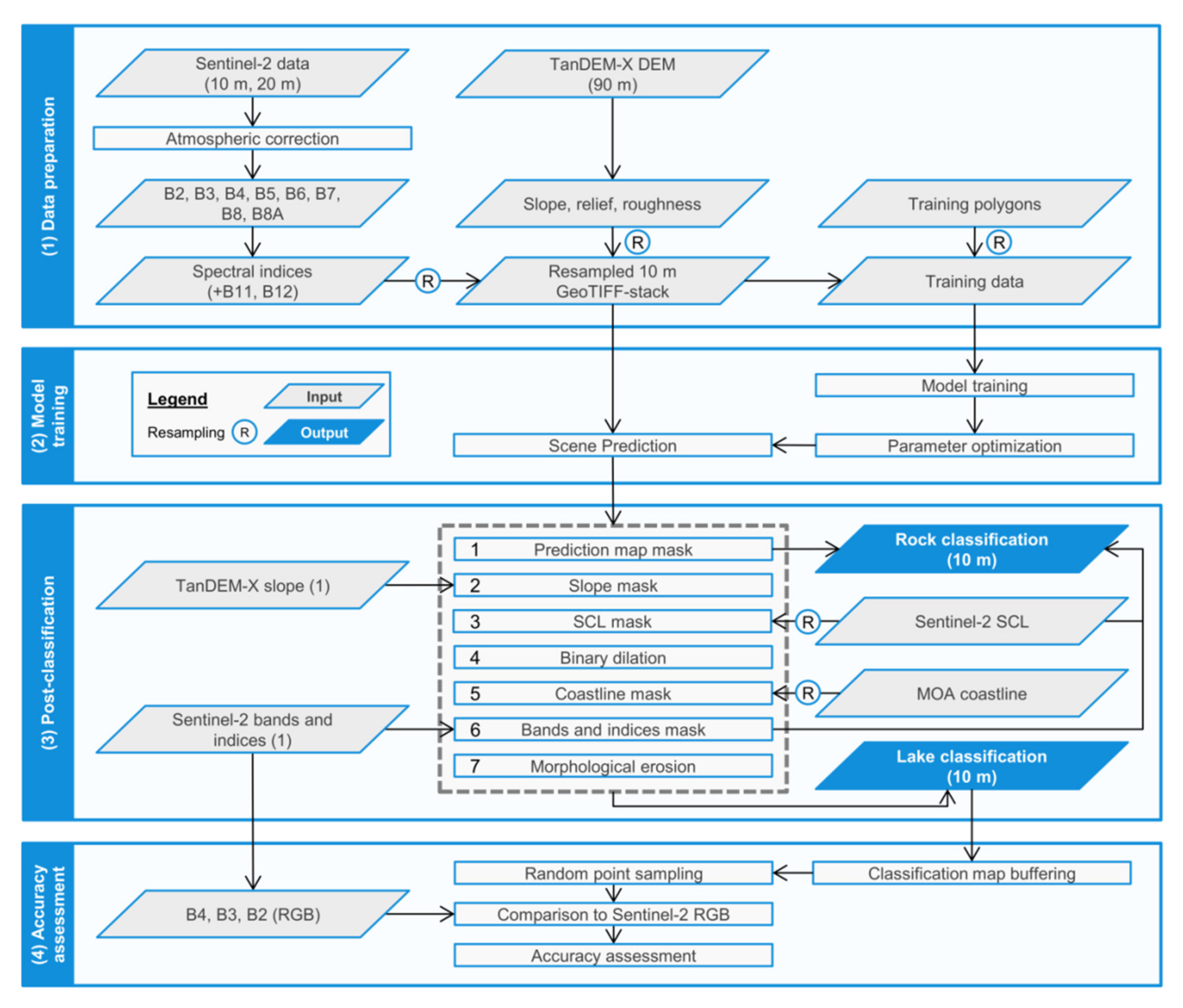
Figure 3.
Overview maps of the study regions. (a) Distribution of training (blue) and test (red) sites across the Antarctic continent. (b) Spatial coverage of Sentinel-2 acquisitions covering the Amery Ice Shelf during the 2017, 2018, 2019 and 2020 melt seasons as well as their overlap area and Region of Interest (ROI) 1. GL = Grounding Line. The coastline data were downloaded from the SCAR Antarctic Digital Database (ADD) [50].


Figure 4.
Distribution of pixel values according to their class membership. (a) B2: Blue reflectance. (b) B3: Green reflectance. (c) B4: Red reflectance. (d) B5: Red Edge 1. (e) B6: Red Edge 2. (f) B7: Red Edge 3. (g) B8: NIR. (h) B8A: Red Edge 4. (i) NDWI1. (j) NDWI2. (k) NWI. (l) AWEIsh. (m) AWEInsh. (n) TCwet. (o) NDSI. (p) SWI. (q) NDGI. (r) SAVI. (s) SI. (t) NDI. (u) DEM. (v) Slope. (w) Relief. (x) Roughness. The boxplots show the interquartile ranges, the median, the range of the data as well as outliers. In (a–h), the y-axes show the Sentinel-2 surface reflectance values for each band and in (i–t) and (u–x), the y-axes represent normalized indices and scaled representations of the topographic layers respectively.
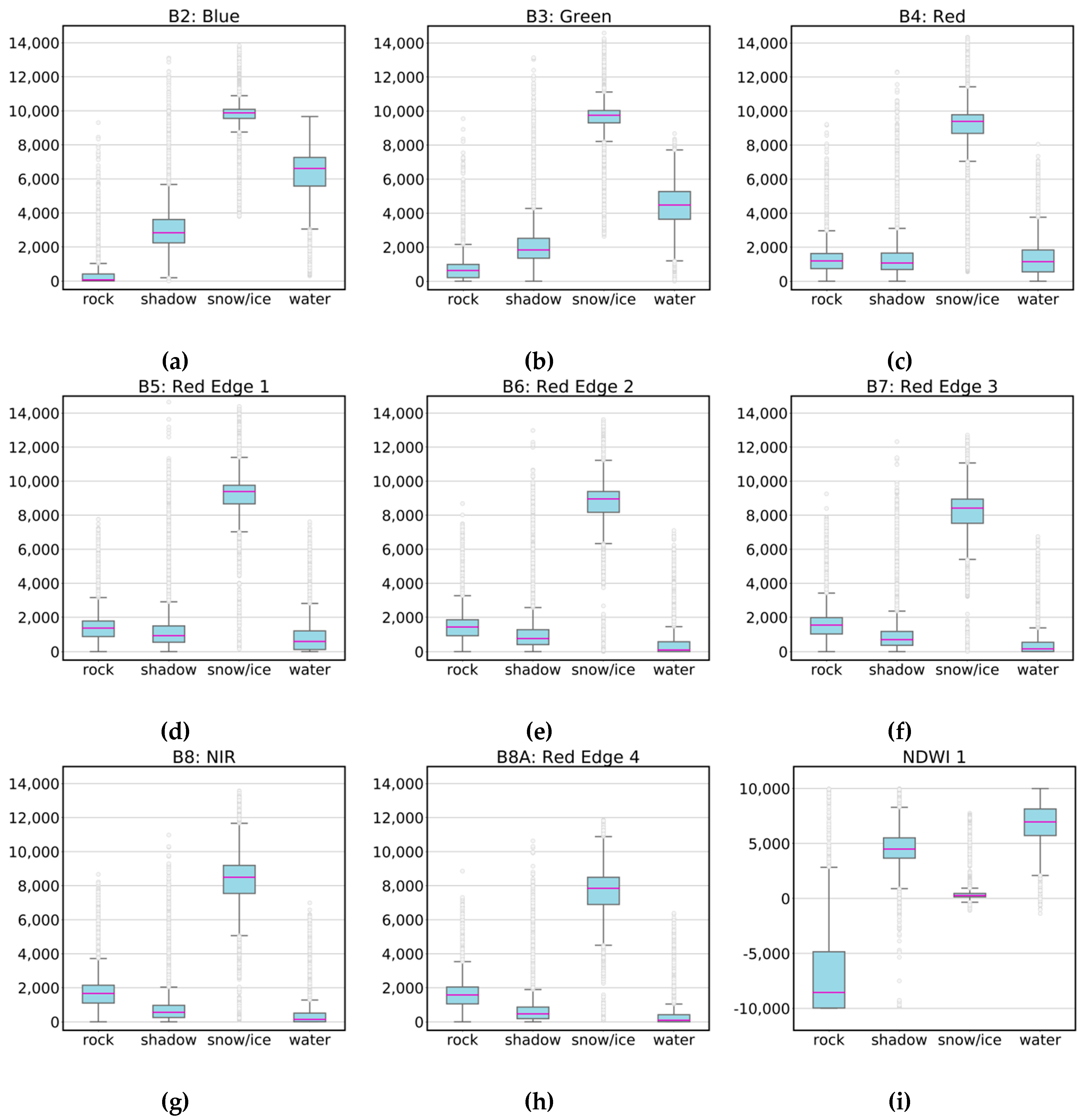

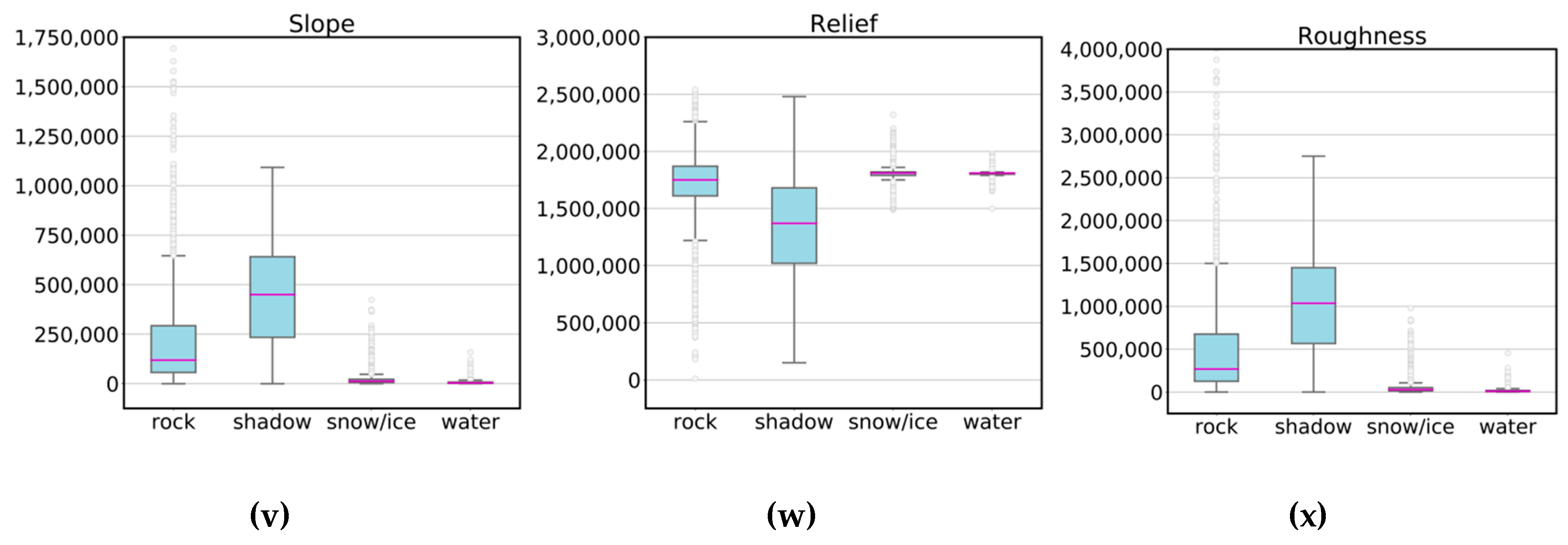
Figure 5.
Feature importances for the Random Forest (RF) training variables averaged over all training regions and classes.
Figure 5.
Feature importances for the Random Forest (RF) training variables averaged over all training regions and classes.

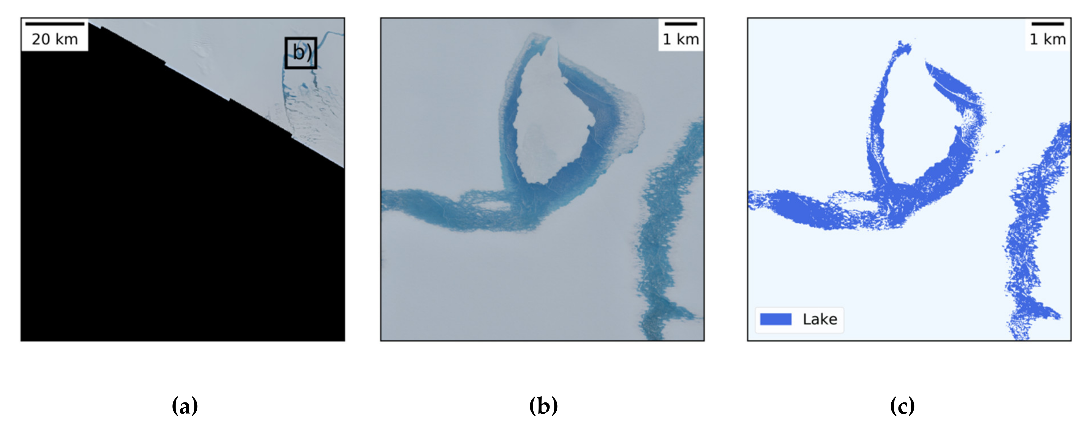
Figure 6.
Sentinel-2 test scenes (a,d,g,j,m,p,s,v), image extracts (b,e,h,k,n,q,t,w) and final automated mapping results (c,f,i,l,o,r,u,x) for all test regions. (a–c) Nivlisen Ice Shelf. (d–f) Amundsen Bay. (g–i) Wilhelm II Coast. (j–l) Drygalski Ice Tongue. (m–o) Hull Glacier. (p–r) Abbott Ice Shelf. (s–u) Cosgrove Ice Shelf. (v–x) George VI Ice Shelf. The red boxes in (s) show the regions analyzed in Figure 7.


Figure 7.
Sentinel-2 extracts of regions 1 (a) and 2 (d) within the test scene of Cosgrove Ice Shelf, West Antarctic Ice Sheet (WAIS) (see Figure 6s). (b,e) Classification maps before coastline (b) as well as bands and indices (e) masking as part of postclassification. (c,f) Classification maps after automated postclassification.

Figure 8.
Maximum lake extent and rock outcrop maps for ROI 1 over Amery Ice Shelf during the 2017 (a), 2018 (b), 2019 (c) and 2020 (d) melt seasons.
Figure 8.
Maximum lake extent and rock outcrop maps for ROI 1 over Amery Ice Shelf during the 2017 (a), 2018 (b), 2019 (c) and 2020 (d) melt seasons.
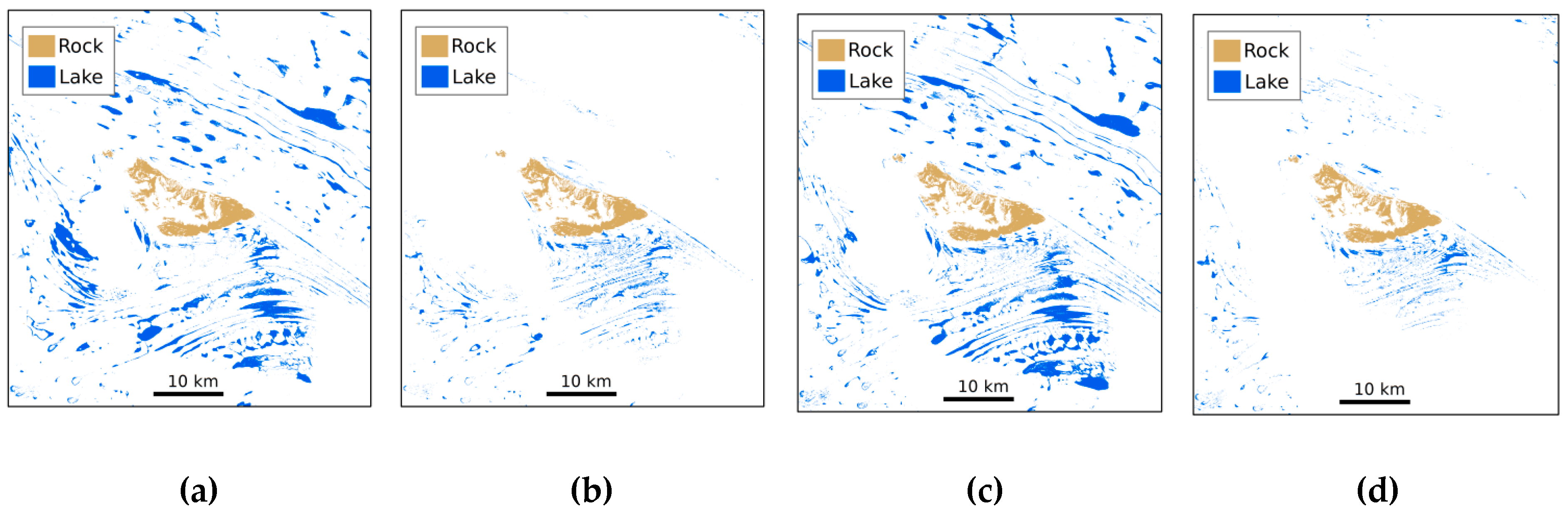
Figure 9.
Maximum extent of supraglacial lakes on Amery Ice Shelf during the 2017, 2018, 2019 and 2020 melt seasons with respect to the total coverage of Sentinel-2 acquisitions for each year (blue), their respective overlap region (green) as well as ROI 1 (red).
Figure 9.
Maximum extent of supraglacial lakes on Amery Ice Shelf during the 2017, 2018, 2019 and 2020 melt seasons with respect to the total coverage of Sentinel-2 acquisitions for each year (blue), their respective overlap region (green) as well as ROI 1 (red).
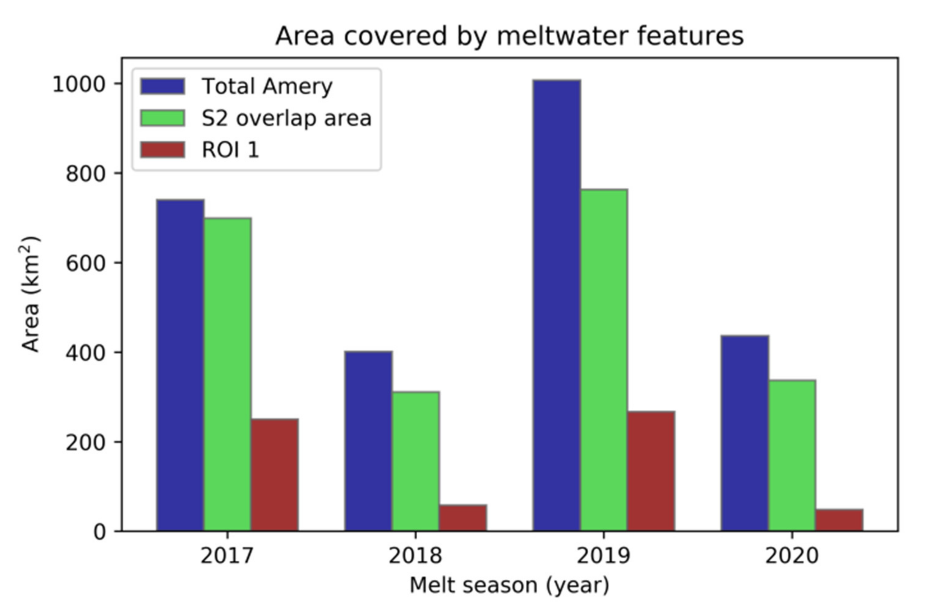
Figure 10.
Maximum lake extent and rock outcrop map for the full Sentinel-2 coverage during the 2019 melt season over Amery Ice Shelf, Antarctica.
Figure 10.
Maximum lake extent and rock outcrop map for the full Sentinel-2 coverage during the 2019 melt season over Amery Ice Shelf, Antarctica.


Table 1.
Sentinel-2 data used for training and test regions.
| Number | Date | Relative Orbit | Study Area | Study Region |
|---|---|---|---|---|
| (1) Training Region | ||||
| 1 | 02 February 2017 | 7 | Riiser-Larsen Ice Shelf | EAIS |
| 2 | 21 January2019 | 49 | Nivlisen Ice Shelf | EAIS |
| 3 | 14 January 2019 | 91 | Roi Baudouin Ice Shelf | EAIS |
| 4 | 04 February 2019 | 105 | Shirase Bay | EAIS |
| 5 | 17 January 2019 | 133 | Mawson Coast | EAIS |
| 6 | 02 January 2019 | 61 | Amery Ice Shelf | EAIS |
| 7 | 13 January 2019 | 75 | Amery Ice Shelf | EAIS |
| 8 | 11 February 2019 | 61 | Amery Ice Shelf | EAIS |
| 9 | 13 January 2019 | 75 | Publications Ice Shelf | EAIS |
| 10 | 29 January 2019 | 17 | Shackleton Ice Shelf | EAIS |
| 11 | 02 January 2019 | 71 | Nordenskjöld Ice Tongue | EAIS |
| 12 | 27 January 2018 | 139 | Pine Island Bay | WAIS |
| 13 | 28 January 2019 | 9 | George VI Ice Shelf | API |
| 14 | 24 January 2019 | 95 | Wilkins Ice Shelf | API |
| (2) Test Region | ||||
| 1 | 28 January 2018 | 6 | Nivlisen Ice Shelf | EAIS |
| 2 | 04 January 2017 | 19 | Amundsen Bay (Enderby Land) | EAIS |
| 3 | 14 January 2018 | 89 | Wilhelm II Coast | EAIS |
| 4 | 06 January 2017 | 57 | Drygalski Ice Tongue | EAIS |
| 5 | 23 January 2018 | 83 | Hull Glacier | WAIS |
| 6 | 12 January 2017 | 139 | Abbott Ice Shelf | WAIS |
| 7 | 12 January 2017 | 139 | Cosgrove Ice Shelf | WAIS |
| 8 | 04 February 2018 | 109 | George VI Ice Shelf | API |
Table 2.
Sentinel-2 Multispectral Instrument (MSI) spectral bands at 10 m, 20 m and 60 m spatial resolution.
Table 2.
Sentinel-2 Multispectral Instrument (MSI) spectral bands at 10 m, 20 m and 60 m spatial resolution.
| Band Number | Band Description 1 | Central Wavelength S2A/S2B 2 (nm) | Bandwidth S2A/S2B (nm) | Spatial Resolution (m) |
|---|---|---|---|---|
| 1 | Aerosols | 442.7/442.2 | 21/21 | 60 |
| 2 | Blue | 492.4/492.1 | 66/66 | 10 |
| 3 | Green | 559.8/559.0 | 36/36 | 10 |
| 4 | Red | 664.6/664.9 | 31/31 | 10 |
| 5 | Red Edge 1 | 704.1/703.8 | 15/16 | 20 |
| 6 | Red Edge 2 | 740.5/739.1 | 15/15 | 20 |
| 7 | Red Edge 3 | 782.8/779.7 | 20/20 | 20 |
| 8 | NIR | 832.8/832.9 | 106/106 | 10 |
| 8A | Red Edge 4 | 864.7/864.0 | 21/22 | 20 |
| 9 | Water vapor | 945.1/943.2 | 20/21 | 60 |
| 10 | Cirrus | 1373.5/1376.9 | 31/30 | 60 |
| 11 | SWIR1 | 1613.7/1610.4 | 91/94 | 20 |
| 12 | SWIR2 | 2202.4/2185.7 | 175/185 | 20 |
1. NIR: Near-Infrared, SWIR: Shortwave Infrared; 2. S2A: Sentinel-2A, S2B: Sentinel-2B.
Table 3.
Sentinel-2 derived indices used for supraglacial lake detection with the Random Forest classifier.
Table 3.
Sentinel-2 derived indices used for supraglacial lake detection with the Random Forest classifier.
| Feature | Index | Mathematic Formulation 1 | References |
|---|---|---|---|
| 1 | NDWI1 | [30,54] | |
| 2 | NDWI2 | [55] | |
| 3 | NWI | [56] | |
| 4 | AWEIsh | [59] | |
| 5 | AWEInsh | [59] | |
| 6 | TCwet | [57,58] | |
| 7 | NDSI/MNDWI | [61,62] | |
| 8 | SWI | [63] | |
| 9 | NDGI | [64] | |
| 10 | SAVImod | [60] | |
| 11 | SImod | [65] | |
| 12 | NDI | - |
1.: surface reflectance of respective band.
Table 4.
Area covered by supraglacial meltwater features within the full Sentinel-2 test scenes.
| Test Scene | Region | Area [km2] |
|---|---|---|
| 1 | Nivlisen Ice Shelf | 28.96 |
| 2 | Amundsen Bay | 12.64 |
| 3 | Wilhelm II Coast | 1.16 |
| 4 | Drygalski Ice Tongue | 24.52 |
| 5 | Hull Glacier | 0.97 |
| 6 | Abbott Ice Shelf | 0.81 |
| 7 | Cosgrove Ice Shelf | 1.05 |
| 8 | George VI Ice Shelf | 28.1 |
Table 5.
Supraglacial lake occurrence within defined geographical units on Amery Ice Shelf between 2017 and 2020.
Table 5.
Supraglacial lake occurrence within defined geographical units on Amery Ice Shelf between 2017 and 2020.
| Geographical Unit | ||||
|---|---|---|---|---|
| Distance to Grounding Line ≤10 km | Distance to Coastline ≥300 km | Distance to Rock Outcrop ≤5 km | On Floating Ice Shelf | |
| Year | Number of Supraglacial Lakes [%] | |||
| 2017 | 48 | 61 | 24 | 87 |
| 2018 | 74 | 59 | 58 | 72 |
| 2019 | 53 | 52 | 35 | 81 |
| 2020 | 74 | 67 | 56 | 71 |
Table 6.
Results of the accuracy assessment for the Sentinel-2 test scenes. For each test scene, the columns present the Error of Omission (EO), the Error of Commission (EC), the Recall (R), the Precision (P), the F-measure (F1), the Kappa statistics (K) as well as their average values.
Table 6.
Results of the accuracy assessment for the Sentinel-2 test scenes. For each test scene, the columns present the Error of Omission (EO), the Error of Commission (EC), the Recall (R), the Precision (P), the F-measure (F1), the Kappa statistics (K) as well as their average values.
| Classes | Water | Nonwater | Both | ||||||||
|---|---|---|---|---|---|---|---|---|---|---|---|
| Accuracy Metrics | EO [%] | EC [%] | R [%] | P [%] | F1 [%] | EO [%] | EC [%] | R [%] | P [%] | F1 [%] | K |
| Nivlisen Ice Shelf | 3.16 | 8.00 | 96.84 | 92.00 | 94.36 | 0.88 | 0.33 | 99.12 | 99.67 | 99.39 | 0.938 |
| Amundsen Bay | 20.37 | 6.52 | 79.63 | 93.48 | 86.00 | 0.15 | 0.56 | 99.85 | 99.44 | 99.64 | 0.856 |
| Wilhelm II Coast | 17.14 | 9.38 | 82.86 | 90.63 | 86.57 | 0.15 | 0.30 | 99.85 | 99.70 | 99.77 | 0.863 |
| Drygalski Ice Tongue | 16.67 | 0.00 | 83.33 | 100.00 | 90.91 | 0.00 | 0.36 | 100.00 | 99.64 | 99.82 | 0.907 |
| Hull Glacier | 35.29 | 50.00 | 64.71 | 50.00 | 56.41 | 0.55 | 0.30 | 99.45 | 99.70 | 99.57 | 0.560 |
| Abbott Ice Shelf | 30.99 | 0.00 | 69.01 | 100.00 | 81.67 | 0.00 | 1.13 | 100.00 | 98.87 | 99.43 | 0.811 |
| Cosgrove Ice Shelf | 10.45 | 0.00 | 89.55 | 100.00 | 94.49 | 0.00 | 0.36 | 100.00 | 99.64 | 99.82 | 0.943 |
| George VI Ice Shelf | 3.91 | 0.00 | 96.09 | 100.00 | 98.01 | 0.00 | 0.27 | 100.00 | 99.73 | 99.87 | 0.979 |
| Average | 17.25 | 9.24 | 82.75 | 90.76 | 86.05 | 0.22 | 0.45 | 99.78 | 99.55 | 99.66 | 0.857 |
© 2020 by the authors. Licensee MDPI, Basel, Switzerland. This article is an open access article distributed under the terms and conditions of the Creative Commons Attribution (CC BY) license (http://creativecommons.org/licenses/by/4.0/).
Share and Cite
MDPI and ACS Style
Dirscherl, M.; Dietz, A.J.; Kneisel, C.; Kuenzer, C. Automated Mapping of Antarctic Supraglacial Lakes Using a Machine Learning Approach. Remote Sens. 2020, 12, 1203. https://0-doi-org.brum.beds.ac.uk/10.3390/rs12071203
AMA Style
Dirscherl M, Dietz AJ, Kneisel C, Kuenzer C. Automated Mapping of Antarctic Supraglacial Lakes Using a Machine Learning Approach. Remote Sensing. 2020; 12(7):1203. https://0-doi-org.brum.beds.ac.uk/10.3390/rs12071203
Chicago/Turabian StyleDirscherl, Mariel, Andreas J. Dietz, Christof Kneisel, and Claudia Kuenzer. 2020. "Automated Mapping of Antarctic Supraglacial Lakes Using a Machine Learning Approach" Remote Sensing 12, no. 7: 1203. https://0-doi-org.brum.beds.ac.uk/10.3390/rs12071203
Note that from the first issue of 2016, this journal uses article numbers instead of page numbers. See further details here.