Super-Resolution for Hyperspectral Remote Sensing Images Based on the 3D Attention-SRGAN Network


Guangdong Key Laboratory for Urbanization and Geoslimulation, School of Geography and Planning, Sun Yat-sen University, Guangzhou 510275, China
*
Author to whom correspondence should be addressed.
Remote Sens. 2020, 12(7), 1204; https://0-doi-org.brum.beds.ac.uk/10.3390/rs12071204
Submission received: 6 March 2020
/
Revised: 5 April 2020
/
Accepted: 6 April 2020
/
Published: 8 April 2020
(This article belongs to the Section Remote Sensing Image Processing)
Abstract
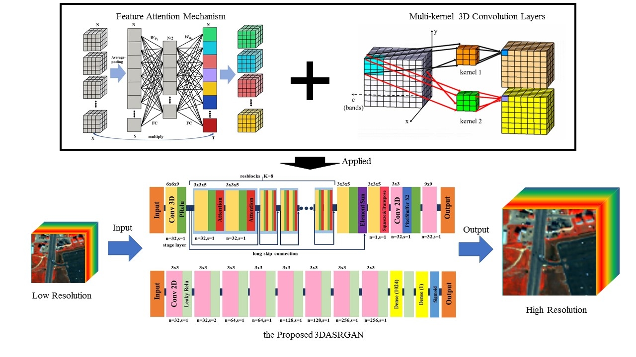
:Hyperspectral remote sensing images (HSIs) have a higher spectral resolution compared to multispectral remote sensing images, providing the possibility for more reasonable and effective analysis and processing of spectral data. However, rich spectral information usually comes at the expense of low spatial resolution owing to the physical limitations of sensors, which brings difficulties for identifying and analyzing targets in HSIs. In the super-resolution (SR) field, many methods have been focusing on the restoration of the spatial information while ignoring the spectral aspect. To better restore the spectral information in the HSI SR field, a novel super-resolution (SR) method was proposed in this study. Firstly, we innovatively used three-dimensional (3D) convolution based on SRGAN (Super-Resolution Generative Adversarial Network) structure to not only exploit the spatial features but also preserve spectral properties in the process of SR. Moreover, we used the attention mechanism to deal with the multiply features from the 3D convolution layers, and we enhanced the output of our model by improving the content of the generator’s loss function. The experimental results indicate that the 3DASRGAN (3D Attention-based Super-Resolution Generative Adversarial Network) is both visually quantitatively better than the comparison methods, which proves that the 3DASRGAN model can reconstruct high-resolution HSIs with high efficiency.

1. Introduction
A hyperspectral image (HSI) is a three-dimensional data cube that records a set of two-dimensional images (or bands), which represent the reflectance or radiance of a scene at various electromagnetic wavelengths [1]. Unlike other forms of images, HSIs can provide a wider range of spectral information, which can be used to distinguish the objects in the image scene. They have been extensively employed in fields such as military object recognition [2], geological exploration [3], and target detection [4]. However, the spatial resolution of HSIs is rather low compared to multispectral images. This is because when applied to the same region of the electromagnetic spectrum as multispectral sensors, hyperspectral sensors capture bands with higher density. Therefore, only a relatively small number of photons are collected within each narrowed band. To reduce the proportion of noise in the collected information, a relatively large area of spectral information needs to be gathered together so it can be strong enough to be detected, which will trade off spatial resolution [5]. In these low-spatial-resolution images, it is very hard to utilize the spatial feature to identify objects on the ground with acceptable accuracy, which limits the applications of HSIs. In this case, how to reconstruct HSIs into high-resolution images is a significant task.
Image super-resolution (SR) is proposed to reconstruct the corresponding high-resolution (HR) image from the observed indistinct low-resolution (LR) image [6]. It is more economical to directly utilize an image processing method to improve the resolution of images and also very helpful to recover the images captured by existing LR imaging systems [7].
Great innovation and successful progress have been made in recent years in dealing with the SR problems. There are two ways to solve SR problems in general, namely, the fusion HSI SR method and the single HSI SR (SISR) method. The fusion method combines information from images with high spatial resolution and low spectral resolution (such as the panchromatic image or multispectral image) with the target image to reconstruct the HR HSI. This method has been proven to be useful in several research studies [8,9,10,11,12,13,14,15]. Many research papers focus on how to better restore image quality [16] and fuse various information of such data [17,18,19]. However, owing to the differences in imaging sensors and collecting time of these images, the auxiliary images are not always available for the fusion process. Therefore, the SISR method is increasingly gaining attention among researchers.
The improvement in computing power brought by the advancement of computer technology and the emergence of more avant-garde ideas have made SISR based on machine learning methods flourish in recent years. Deep learning is one of the most effective methods and many research achievements have accomplished on its basis [20]. The application of deep learning in SR was first proposed by Dong et al. [13]. They proposed a state-of-the-art Super-Resolution Convolutional Neural Network (SRCNN) model, which is easy to train and works well. However, it only uses one layer of convolution layer for the feature extraction, thus, there is a small perceptive field problem, that is, the extracted features are very local and it does not lay emphasize on the spectral dimension. In order to enhance the SR effect on the texture details of the images, Kim et al. [21] designed a deep SR VGG (visual geometry group) network that combined VGGnet [22] with SRCNN. By using this method, the SR images can achieve a better performance in the aspect of texture and details. Nevertheless, deep networks would bring more parameters and slow the efficiency. Similar research has been conducted in [23,24,25]. One problem of these methods is that they focus on SR for RGB images, which may not perform well for HSIs with many interlinked bands. To address this problem, Han et al. [26] developed a model using spatial and spectral fusion with CNN for HSI SR. CNN has some limitations in feature extraction: it only has receptive field on the spatial dimension, thus, the feature may not be fully extracted, which would weaken the impact of SR result. In another study, Luo et al. [27] developed a network HSI-CNN for HSIs by making use of the deep residual convolutional neural network (ResNet). In this network, they applied the ResNet structure in some layers and added spectral loss in the pixel space to quantify both spatial and spectral quality. The reconstruction results indicated a high signal-to-noise ratio and good image quality, particularly in the spectral dimension. Moreover, Mei et al. [28] made full use of the characteristics of three-dimensional (3D) convolution to extract the features between the bands for SR, and found that 3D convolution could effectively deal with the spectral problem for SR. It is an inspiring method to solve the problem that arises in traditional two-dimensional (2D) convolution: that it cannot get good feature extraction in the spectral dimension. However, their network structure is based on SRCNN, which is not a map-to-map structure, and limits the input and performance of SR.
The generative adversarial networks (GAN) framework developed by Goodfellow et al. [29] has provided more possibilities for the exploration of SR methods. Ledig et al. [30] proposed the SRGAN framework based on the framework of GAN, which demonstrated a remarkable performance in SR. In their work, they employed a perceptual-driven content loss, rather than remaining confined to the similarity in the pixel space. SRGAN could reconstruct most of the detailed contents of an image. Thus, the SR result displayed good visual effects and high quality. However, the SRGAN is developed for handling the SR problem of natural images, and it only requires considering the spatial similarity between the restored and real images. Compared to normal RGB images, HSIs contain much more spectral information, which can be used later to differentiate among various ground objects. Thus, it would cause spectral distortion and information loss if SRGAN is applied directly to the HSI SR problem.
To address the spectral-distortion problem, and to deal with the multiply feature produced by the network, we introduced the 3D convolution into SRGAN. Additionally, we applied the attention mechanism to the network to magnify the contribution of the features that matter; thus, we proposed a novel 3DASRGAN model for the HSI SR problem. Firstly, the original convolution layers in the SRGAN were replaced with 3D convolution layers to solve the spectral distortion problem. 3D convolution layer can extract spectral information from adjacent bands together with spatial context from the neighboring pixels. In this case, the spectral information can be better preserved. Secondly, a spectral loss was introduced into the original loss of the structure to make it applicable to the HSI because SRGAN fails to address the spectral discrepancy when defining the loss function. Spectral loss is defined by the spectral angle (SA), which is used to measure the spectral similarity between the generated image and the original image. The SRGAN network applied the BN layers. However, if the differences between the training set and testing set are obvious, the use of the BN layer could limit the generalization ability of the generator by creating undesirable effects, and this can occur under the GAN framework. Moreover, the HSI dataset contains a relatively small amount of data, so that the advantages of the BN layer could not be maximized. Owing to these reasons, we attempt to improve the networks by removing all the BN layers. Finally, the 3D convolution layers will generate much more features than the normal 2D convolution layers; if we treat them equally, it might not be positive to the network. Thus, a feature attention mechanism was applied to help the network focus on the features that attribute most to the SR task, which causes the network to have the potential of improving the effect of SR and get a better result.
The three main contributions of our research are as follows:
- Our 3DASRGAN model extracts the spatial and spectral features of HSIs using a 3D convolution layer. It can reconstruct the LR HSIs by improving the network structure of the SRGAN to obtain HR HSIs, and most importantly, it helps to minimize the spectral distortion effect of the original SRGAN.
- Our model attaches significance to the spectral similarity between the SR and the original image. With the spectral loss calculated by adding SA to the generator loss function, the SR result is improved in the spectral aspect.
- To better use the extracted features from 3D convolution, we applied the features attention mechanism on every resblock to acquire the accumulated and well-performed feature in the network to improve the ability of the network for SR.
2. Methodology
Traditional super-resolution network models such as SRCNN and SRGAN often employ 2D convolution layers to extract the spatial features of RGB images. These layers pay little attention to the correlation between image bands, thus ignoring spectral information. Therefore, this type of network is suitable only for images with few bands, such as RGB images or single-channel images. If we want to preserve spectral information when dealing with HSI SR problems, we must not only consider the spatial relation of the neighboring pixels, but also the spectral similarity of the neighboring bands. The idea of generating confrontation in SRGAN is very conducive to the detailed reconstruction of images. Drawing on previous studies and combining the characteristics of 3D convolution with the application of attention mechanism, this study proposes a 3D attention-based super-resolution generative adversarial network (3DASRGAN). Because the HSIs obtained by the same sensor have the same distribution in hyper-dimensional space, when we narrow the dataset down to the HSIs obtained by a specific sensor, the 3DASRGAN will have a clearer learning direction. Furthermore, this type of dataset has the same spectral resolution and band numbers, which facilitate the construction of an end-to-end network structure.
2.1. Architecture of the Proposed 3DASRGAN
The 3DASRGAN contains two essential networks, a G(Generator) and a D(Discriminator). In SISR, an LR data cube is the input of G, and represents the corresponding HR image. is the output of G. For a cube with C bands, we usually define by a tensor whose size is W × H × C, in which W and H stand for the weight and height, respectively. We also define and by the size of rW × rH × C, where r represents the scale. Figure 1 illustrates the architecture of the proposed 3DASRGAN.
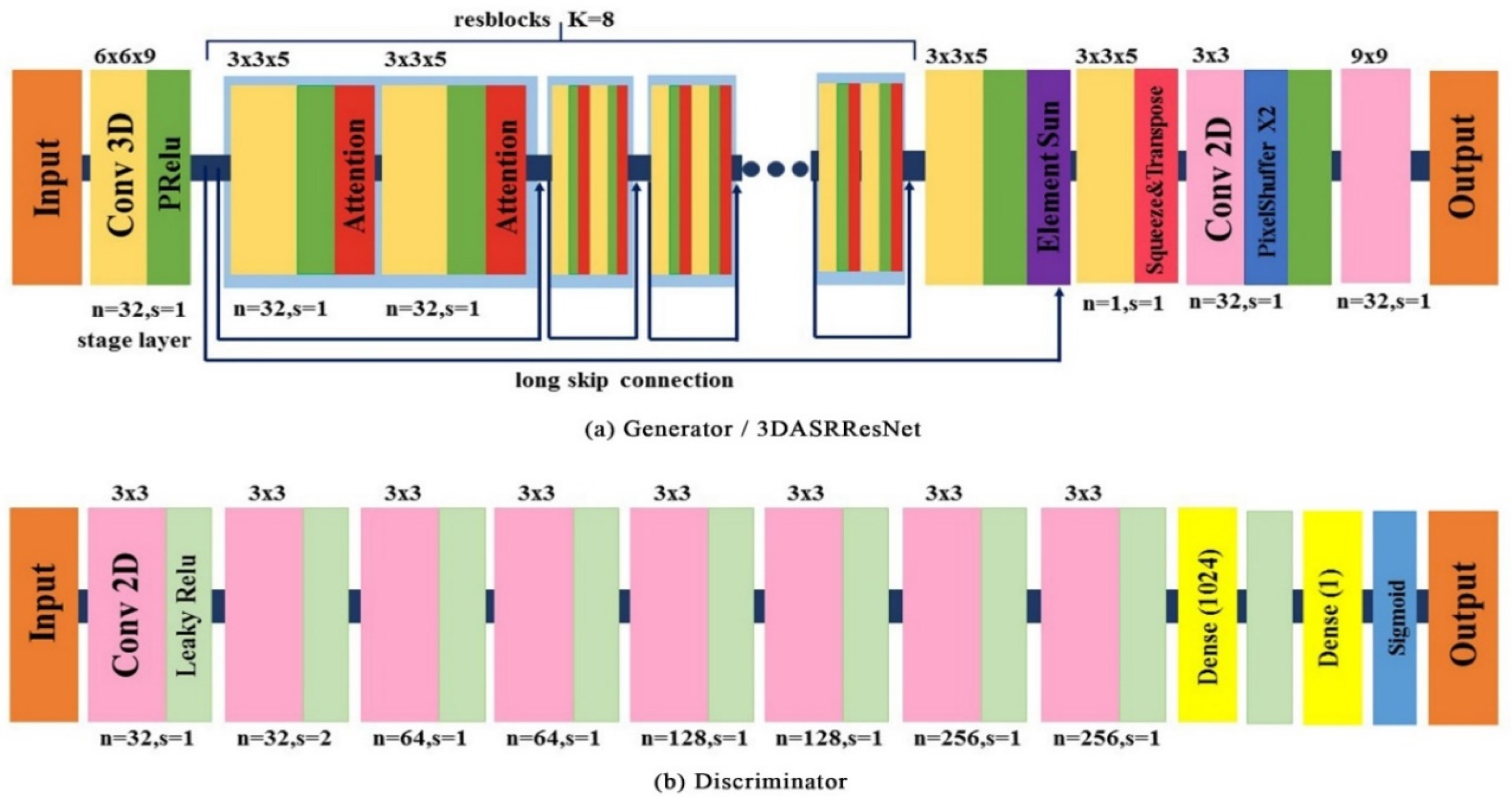
In this paper, the G contains a stage layer, followed by eight resblocks (K = 8). A resblock is composed of two identical parts, each of those contains a 3D convolution followed by an attention layer. There is a short skip connection between the resblocks and a long skip connection between the stage layer output and the results of the resblocks. The summed element goes through a 3D convolution layer first and, subsequently, the output is squeezed into a four-dimensional (4D) tensor that will be transposed before the sub-pixel [22] layer. Finally, a 2D convolution with a large kernel size works on the output tensor of the sub-pixel layer.
For the discriminator, there are eight 2D convolution layers with LeakyReLU activation, followed by two dense layers. The output of the D is the probability for distinguishing the real HR image IHR and the generated image ISR. The details of the framework will be provided in the following section.
2.1.1. Generator Network Architecture
The purpose of the SRGAN network is to train a G that can simulate the corresponding HR HSI from a sensor-specific LR HSI. We assume that the G function is parametrized by , which represents all the weights and biases of the generator. With the training of the LR HSI dataset , together with corresponding HR HSI cubes (i = 1, 2, 3, …), we can solve the following function:
Thereafter, we can obtain the optimized G function (the generator). In Equation (1), is the output of the generator, which can also be described as . As the key process of SR is based on the deep convolution layers in G, 3D convolution is used in G. Generally, an HSI cube in the 3D convolution network is described as a five-dimensional (5D) tensor N × B × H × W × C. N represents the batch size and B is the representative for the depth of the data, which is the band number of the data cube here. When 3D convolution is used for processing the video, C is the number of channels. However, for the HSI dataset, each band has only one channel. Therefore, C equals 1 when the 3D convolution is applied in HSIs. The fundamental architecture of the generator is illustrated in Figure 2, in which a very deep ResNet with eight blocks is used, and each block has an identical layout. Before the deep network in the generator, there is a stage of convolution layer with larger kernels. According to previous research, using a larger kernel layer before the deep network can usually help the network achieve a better result. There is a one-kernel 3D convolution layer that follows the resblocks, and it is used to make the number of channels of the output equal to 1 again. Additionally, a squeeze operation was used to transform the 5D output tensor into a 4D tensor. To enhance the resolution of the input HSI cube, a sub-pixel convolution layer is used in the network. The sub-pixel network was based on 2D convolution; therefore, the input needed to be a 4D tensor. In 2D convolution, the cube is described as a 4D tensor N × H × W × C, where C stands for the number of bands. Thus, following the squeezing operation, the structure of the output cube is N × C × H × W. Therefore, a transpose operation is required before the sub-pixel layer. The detailed structure of the network has shown in Figure 1a.
2.1.2. The Proposed Feature Attention Strategy
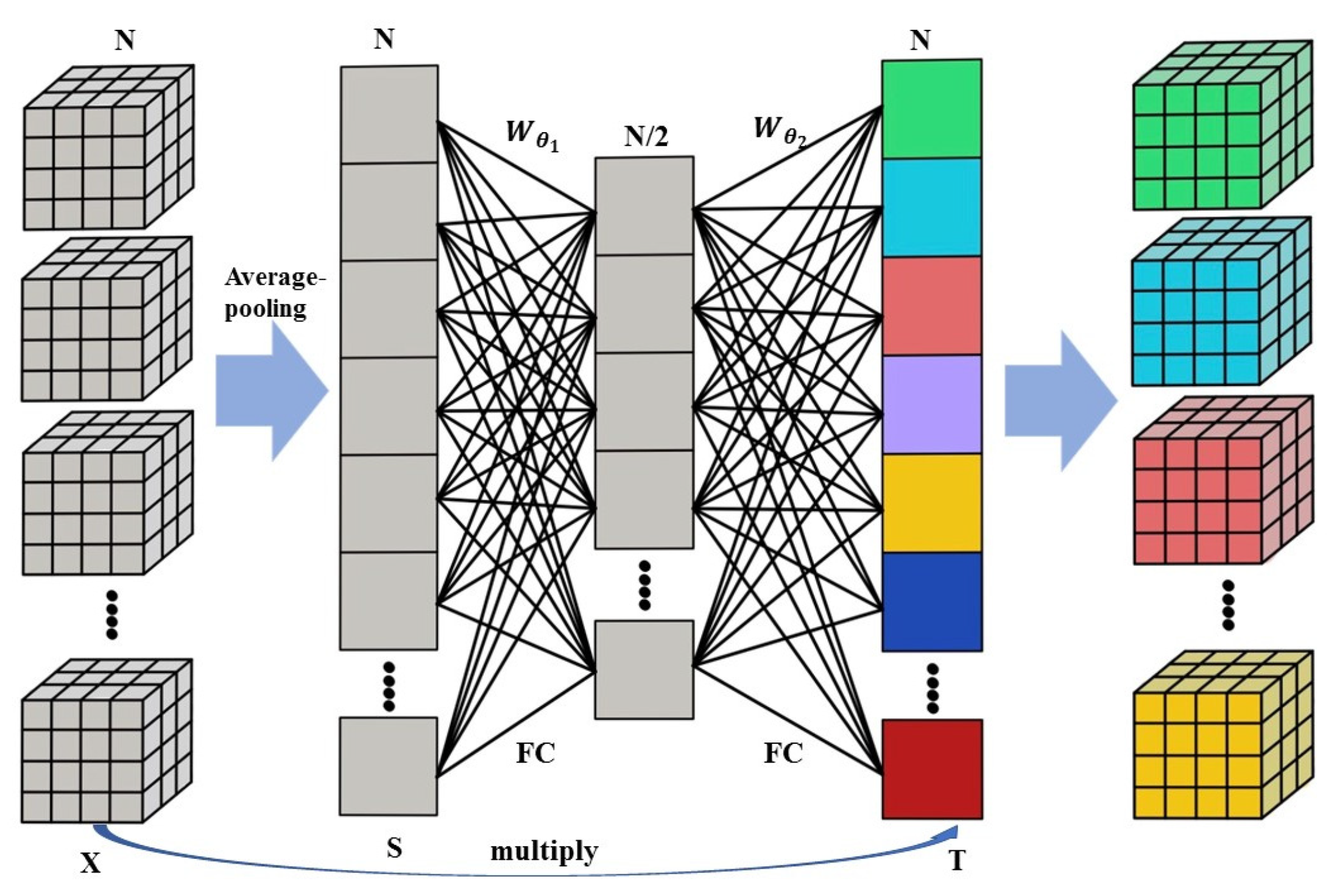
The feature attention mechanism is an in-place module, which means there is no dimension change between the input and output. In the resblocks mentioned in the last section, each contains two attention layers to help the network focuses on the well-performed feature generated by the 3D network layer. We applied a squeeze-and-extracted strategy on the 4D tensor of the 3D network output. Firstly, the network squeezes the 4D tensor into a vector by using the average pooling method. Given the input tensor after the average-pooling, we obtain the global average tensor , where:
and l is the index of the features, C, H and W are the band number, height and width of the tensor. After the average pooling layer, two thin fully connection layers (nonlinear transformation FC layers) are connected, which have a number of neural cell of N/2 and N, respectively. A sigmoid layer was applied to the output vector to make sure every value was in the range of 0 to 1. Thus, this vector represents the scaling coefficient of every feature, where:
and , are the parameters of the fully connection layers. Finally, the output was computed by a multiply operation of the output features and the scaling coefficient T. The detail of the attention strategy is presented in Figure 2, where N represent the number of the features 3D-tensor generated by the 3D convolution layers.
2.1.3. Adversarial Network Architecture
A discriminator network is designed in [29] to solve the adversarial min-max problem:
The general idea behind this formulation is to train the G function with the goal of fooling D, which is used to distinguish the SR image from the real HR image. The stronger the G is, the weaker D’s discrimination ability is. In this way, D encourages G to be optimized and generate images that are highly similar with the real ones.
We expect a fully connected layer in D. Using 2D convolution can save much space that would alternatively be used for storing the weights for D. Therefore, we retained the original architecture of D in the SRGAN and reduce the number of kernels by half. We set α = 2 for LeakyReLU activation, which is used to avoid max-pooling throughout the network. The entire architecture of D is also illustrated in Figure 1b.
2.2. Optimization of 3DASRGAN
For the generator, the defining loss function (G loss) is significant, and it links to the effect of G. The G loss should be designed carefully to quantify the difference between and . MSE (mean squared error) is the general method used to describe the distance between two data points by calculating the square of the difference between the real value and the estimated value; however, this definition focuses only on the distance between two images in the pixel space without emphasizing the essential similarity in spectral dimension in and . Thus, we modified the original G loss by calculating the weighted sum of a spatial loss, a spectral loss and an adversarial loss represented by , and , respectively:
In the following discussion, we will explain how these loss functions are constructed. The pixel-wise MSE is used as the spatial loss, which is calculated as:
This is the most common optimization target for a network. MSE can be calculated and formulated simply; thus, in our study, we consider it the spatial loss.
The spectral loss should be able to measure the spectral similarity. In several studies, the geometric measurement consists of distance and angular measurements. The angular measurement is composed of a high-dimensional vector which is calculated using the origin and high-dimensional space points, and the SA between two high-dimensional vectors is considered as the measuring standard. The formula for calculating SA is:
The smaller SA is, the more similar is the spectrum. Therefore, this formula can be directly considered as a spectral loss.
Adversarial loss is calculated on the discriminator. This loss encourages the generator network to produce a more satisfying solution by fooling the discriminator network. Adversarial loss can be calculated as follows:
where is the discriminator, which can output the probability that the reconstructed image cube is the real HR image .
3. Data Description and Experiment Setting
3.1. Data and Description of Experiment
In this study, we used the Washington DC Mall dataset obtained from the Hydice sensor and the Urban dataset to construct a sensor-specific 3DASRGAN. The wavelengths of the two datasets are both from 0.4–2.5 um. The Washington DC Mall dataset image is a widely-used hyperspectral dataset; it contains 191 bands, formed by removing the H2O, H2, and O2 absorption bands from the original 224 atmospherically corrected bands, and each band has 1280 × 307 pixels. The Urban dataset is also a widely-used hyperspectral dataset. There are 210 bands, 307 × 307 pixels in each band, and each pixel corresponds to a 2 × 2 square meter area. These two datasets are used as the ground truth for HR HSIs, and we used them to train and evaluate the performance of our 3DASRGAN framework.
In this experiment, we divided the dataset into two parts—the larger part was used for training the networks and the remaining was used for testing and evaluating the performance of the networks.
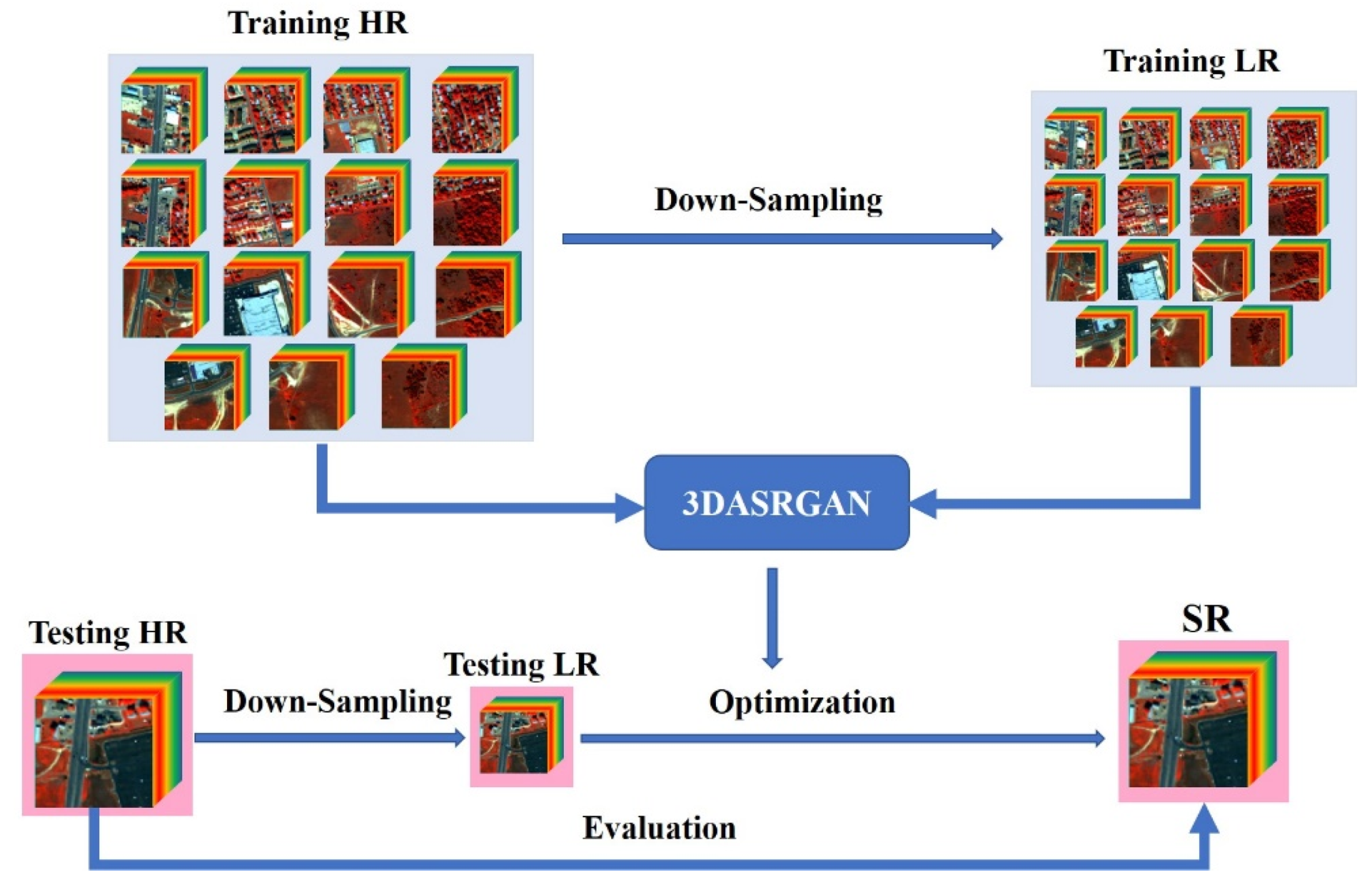
The LR data cube was generated by down-sampling the original dataset by a scale of 2. In general, datasets such as Urban and Washington DC Mall do not have high spatial resolutions. According to existing works, the larger the down-sampling scale is, the harder is the SR process.
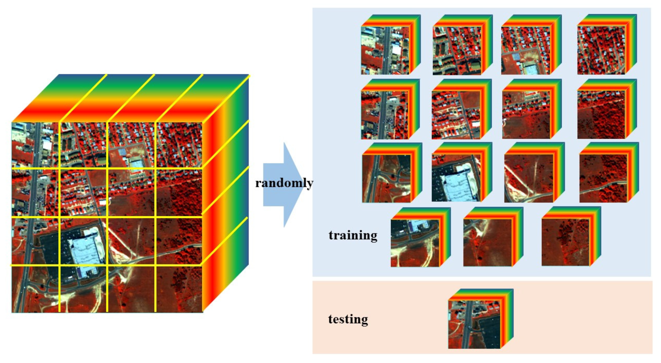
The training procedure can be divided into three steps as below. First, we conducted the preprocessing, in which the dataset was divided into equal parts. Then, we carried out the training by randomly choosing some parts of the dataset and using them to generate and optimize the output of the networks. After that, we tested the networks to see if they are appropriately built. When the networks were built, we applied them to the rest of the dataset and evaluated their impact. The calculation time of the whole experiment was about 22 h.
The whole process of the experiment is depicted in Figure 3.
3.2. Training Details and Parameters
We trained all the networks on an NVIDIA GeForce GTX 1070Ti GPU. We split the DC Mall dataset into 16 equal parts, randomly chose one for testing, and used the rest and their correlative LR for training. For the Urban dataset, every part has 75 × 75 × 210 pixels. For the DC Mall dataset, every part has 150 × 160 × 224 pixels, as shown in Figure 4. The generator network, also known as 3DASRResNet in this study, should be trained independently at first to avoid a local optimum [29]. We limited the range of the LR input image to (0,1) using linear stretching. For the weights of the generator loss, after several batches of experiments, we trained the networks with α = 0.75, β = 0.25, and γ = 0.08. For optimization, we used the Adam (Adaptive Moment Estimation) optimizer [31], setting the parameter to 0.9. The 3DASRResNet was trained with a learning rate of 10−4 and 104 updated iterations. After 5 × 10⁴ steps of training the 3DASRResNet, we collected all the weights and restored them to the generator part of the 3DASRGAN. Next, we trained it for 3 × 10⁴ steps with a learning rate of 10−4 and 104. Goodfellow et al. [29] suggested that in the GAN, the generator, and discriminator should be updated alternately, and the gap steps between each instant of generator and discriminator update should be represented by a parameter k. In our experiment, k = 1. Because the input tensor was very large and required a lot of memory to store, we used only eight identical residual blocks as the original SRGAN in which the number was 16, and thus avoided the “resource–exhausted” error in the training. The same training process was also applied to the Urban dataset for the experiment.
3.3. Evaluation of Performance of 3DASRGAN
To evaluate our framework’s performance accurately, we compared the performance of the 3DASRGAN and the 3DASRResNet with other methods. Two indexes—peak signal-to-noise ratio (PSNR) and structure similarity (SSIM) [32]—were used to quantify the spatial reconstruction quality of the SR image. PSNR is the most popular and widely used objective evaluation index of the image. However, it is only based on the error between corresponding pixels. Because the visual characteristics of human eyes are not considered, the evaluation results are often inconsistent with human subjective feelings. SSIM is mainly used to measure the integrity of image structure, which is another commonly used objective evaluation index. This index takes the structural distortion of the image into account so that it can better reflect the judgment of the human visual system on the similarity of the two images.
The calculation formula for these two indexes is:
MSE is calculated using the formula for . MAXI represents the maximum of the pixel value.
where and represents the mean value of the image and , is the covariance of , and and represent the variance of the image and . Constants c1 and c2 are added to avoid the divide-by-zero error, in which , and usually , by default, and L is the extent of pixel value, which equates to 1 in our study.
To evaluate the spectral reconstruction quality, the spectral angle mapper (SAM) value between the reconstructed SR image and its corresponding ground-truth HR image were used. The SAM value is calculated using the following formula:
In general, higher PSNR and SSIM values imply better visual quality and spatial reconstruction quality, and a lower SAM value implies low spectral distortion and higher spectral reconstruction quality.
4. Result
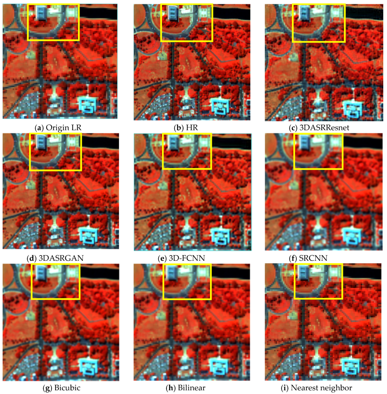
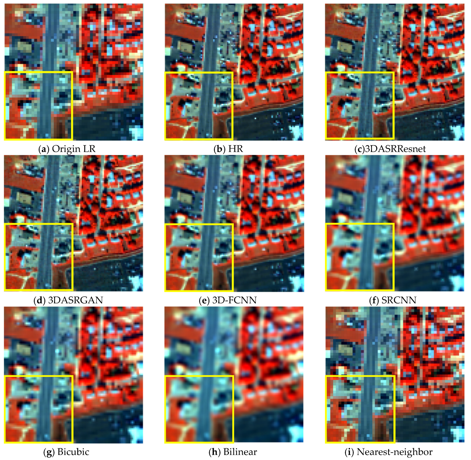
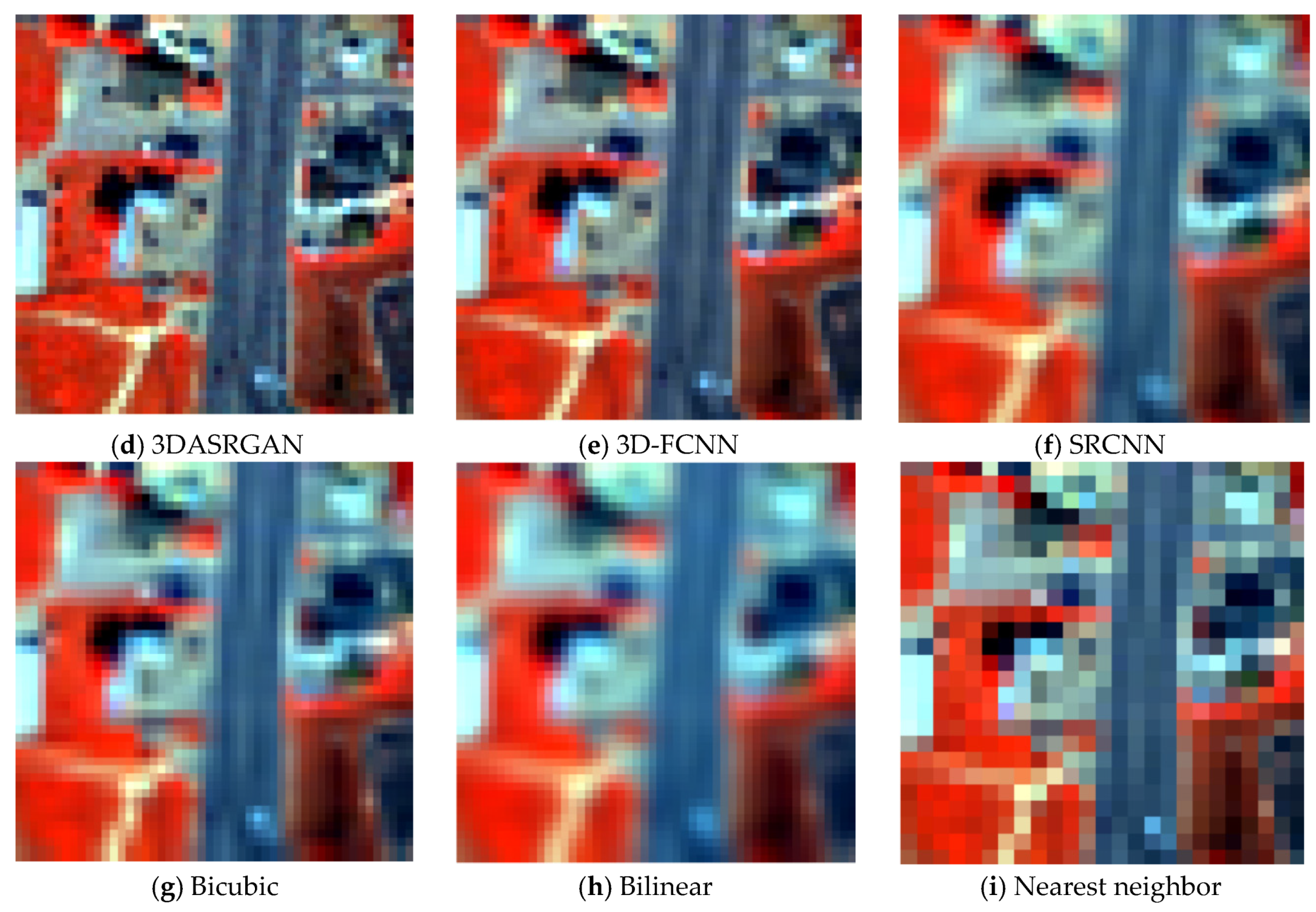
To better evaluate the performance of our 3DASRGAN, we compared our model with several different HSI SR methods, which can be divided into two types. The first type contains machine-learning methods, including 3DASRGAN, 3DASRResNet (which is the G part of the 3DASRGAN model), SRCNN [13], and 3D-FCNN [28]. The second type contains the traditional methods, which include bicubic interpolation, bilinear interpolation, and nearest-neighbor interpolation. These methods are often used when addressing SR HSI problems. The resultant images and the real high-resolution images (ground truth HR) are presented in false color composite to better distinguish different objects and do analysis in Figure 5 and Figure 6.
4.1. Visual Performance Comparison
Figure 5 illustrates all the reconstruction results of the various SR methods. Figure 5c,d demonstrates better visual impacts by 3DASRResnet and 3DASRGAN. In these two images, the contours and shapes of the corresponding ground objects have a relatively high spatial recognition, and there is no significant spatial position error or distortion in the SR image. Among these two images, the result of 3DASRGAN perform better in the spatial details than 3DASRResnet, especially in the edge of the objects such as buildings and roads, which is similar with the HR. Therefore, we know that there is improvement done by the network with D rather than the network that only has the G. Figure 5e also shows a good visual effect but not as good as that of the proposed method. However, Figure 5f does not display a good visual result for SRCNN. Compared to the results obtained from other machine learning methods, the images are more blurred. No clear boundary exists among the various ground objects. Moreover, it is difficult to discern the small differences among various types of the same ground feature, such as in the lower left quarter, which displays a complex of buildings. In Figure 5f, the roofs of the various buildings are not clear but jumble together. In Figure 5g–i, which presents the results of traditional SR methods, the visual impacts are not as good as the others. Among these, the nearest neighbor method has the worst impact, because it is visually the same as the original HR image. The other two methods have the same impact, and their visual impact seems to be better than that produced by the SRCNN method.
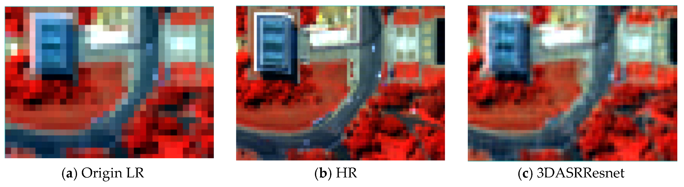
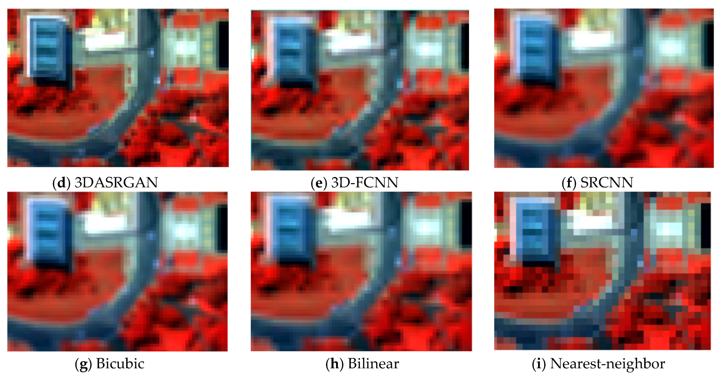
To compare the performance of the various methods in terms of the different objects, we selected an area with a relatively complex spatial texture, including buildings, vegetation, and roads. The results produced by the various methods are presented in Figure 6, which demonstrates that the various methods can create distinct visual impacts on various ground features. To start, let us examine the building parts. In Figure 6d, which presents the results of the 3DASRGAN method, the edges of buildings are the most distinct, and they resemble that of the HR image more. Furthermore, the building contours are also clearly distinguishable with higher resolution. In other images, however, the shapes of buildings are difficult to distinguish. As for roads, we can see from Figure 6b, which presents the HR image, that there are some vehicles on the roads. In the result of 3DASRGAN, the vehicles are most distinguishable. From 3DASRGAN’s result, we can easily identify the boundaries of roads. However, in other images, the roads’ edges become fuzzy and shattered. In images such as Figure 6e–i, the range of pixels occupied by the single-vehicle is larger, and the color of the pixels is closer to the color of the road, which means that it is more difficult to identify the vehicles. Some parts of the roads are difficult to be separated from the vegetation. The restoration of the vegetation is also considered. Because there are some different types of vegetation in this area, the shade of the color should be different; there are also some shadows within the vegetation part. In 3DASRGAN’s result, the heterogeneity among the pixels representing vegetation is the most evident. We can see the light and dark red portions, which represent different types of vegetation, and the parts under the shadow are quite easy to distinguish from the vegetation. Among the results of deep-learning methods, the difference within the vegetation is also clearly presented, although the best effect goes the result of 3DASRGAN. Furthermore, among the results of traditional methods, the difference between the vegetation, even that under the shadows, is not evident, which indicates that these methods are not effective in identifying the plant types. Thus, from the detailed part, it is clearly showed that SRGAN has the best visual impact.
The results from the other dataset, Urban, also demonstrate a similar performance as dataset DC mall. Figure 7 provide a visual presentation of different SR method in false color, which demonstrates that the results of the machine-learning methods provide better visual impacts. In this testing area, roads and buildings have the most distinguishable features, which can easily reflect the visual impact of the SR by comparing the clarity of road and building edges. In Figure 7c–e, the results of 3DASRGAN, SRResNet, and 3D-FCNN stand out as the most similar with the ground truth. As it shows in the images, the result of 3DASRGAN has the best visual effect, which demonstrates the reconstruction ability to the details in the areas with fragmented objects. The edge of the roads are sharp and different objects do not mix together, especially for vegetation and buildings. The image produced by SRCNN, however, is slightly fuzzy in some parts; especially in the junction of vegetation, buildings, and roads, some pixels are mixed and are hard to distinguish from one another. Figure 7g–i demonstrates that the three traditional methods, Nearest, Bilinear, and Bicubic, have the most unsatisfying visual impacts. The image produced by the Nearest method is very fuzzy, and that makes it very difficult to distinguish the features; in some way it is also suggesting that those tradition method for up-sampling are not suitable for the SR of such images with abundant spectral information.
Figure 8 displays the local scene of the testing area that contains typical ground objects as buildings, vegetation, and roads. From these results, we can distinguish between the impacts of these methods more carefully. First, the edges of roofs in the HR image contain light and dark colors, but in Figure 8f–i, which present the images produced using the nearest neighbor, bilinear, bicubic, and SRCNN methods, the differences are eliminated and the color of edges is the same; furthermore, they do not resemble the HR image. The edges of the roads and roofs are roughly showed as the edges of pixels rather than their natural forms. Moreover, the vegetation part of the HR image has different colors. However, in Figure 8f–i, the color of the pixels representing vegetation is nearly the same, blending in with the building pixels, along with some obvious noise. In Figure 8c–e, the heterogeneity within the vegetation is better preserved. Moreover, roads are much clearer in these images. In other images, roads are difficult to distinguish and appears to be broken.
4.2. Quantitative Comparison
We chose three measurement values—PSNR, SSIM, and SAM—to estimate the quantitative similarity for the methods discussed.
The higher the value of PSNR is, the higher the proportion of effective information in the image is, and thus, the better the image quality is. According to Table 1 and Table 2, the PSNR values of 3DASRGAN, 3DASRResNet, and 3D-FCNN are the highest, which indicate that the images reconstructed by these three methods can more effectively reflect the real surface conditions. The PSNR value of SRCNN is smaller than that of other machine-learning-based methods; in other words, the response-ability to the real information of ground objects is not good enough, which reflects that the method used for SR for traditional images with fewer wavebands is not suitable for hyperspectral reconstruction. Among the results of the traditional methods, the Bicubic and Bilinear methods both result in high PSNR and SSIM values; however, their results are worse than those of 3DASRGAN and 3DASRResNet.
SSIM is used to compare the image distortion from three levels: brightness, contrast, and structure. It mainly aims at evaluating the visual quality of images. The higher the value is, the higher the image visual quality is. Among the machine learning methods, the highest SSIM value goes to the 3DASRGAN method, representing the superiority of the 3DASRGAN model from the visual aspect. The SSIM values of 3DASRResNet, 3D-FCNN, and SRCNN all show relatively high results. It means that these models can all obtain fine results in terms of human visual effects, but their results are not as excellent and steady as that of the 3DASRGAN model. Compared with machine learning methods, the results of traditional methods are not effective in representing the good visual effect, as the SSIM values of these models are quite low.
According to Table 1 and Table 2, the highest PSNR and SSIM values are also obtained from 3DASRGAN, and the results obtained from 3DASRResNet and 3D-FCNN are also relatively high. However, the SRCNN method does not achieve a good result compared to other machine learning methods, thus, this method is not effective when dealing with the HSI SR problem. Among the results of the traditional methods, the Bicubic and Bilinear methods both result in high PSNR and SSIM values; however, their results are worse than those of 3DASRGAN and 3DASRResNet.
For HSIs, spectral information is essential. Therefore, the impact of spectral reconstruction cannot be ignored. When the SAM value is closer to 0, it indicates that the SR image is close to HR in the spectral dimension. As listed in Table 1 and Table 2, the 3DASRResNet and 3DASRGAN methods have the lowest SAM values; thus, these two methods are more accurate in terms of the spectrum. For the performance of PSNR and SSIM, the results of 3D-FCNN are also good; however, it is far inferior to the 3DASRResNet and 3DASRGAN methods for the value of SAM. The SAM value of the SRCNN method is the highest among the results of machine learning methods. However, compared with the results of non-machine-learning methods, we can see from Table 1 and Table 2 that the machine-learning methods all perform better in the restoration of spectral information.
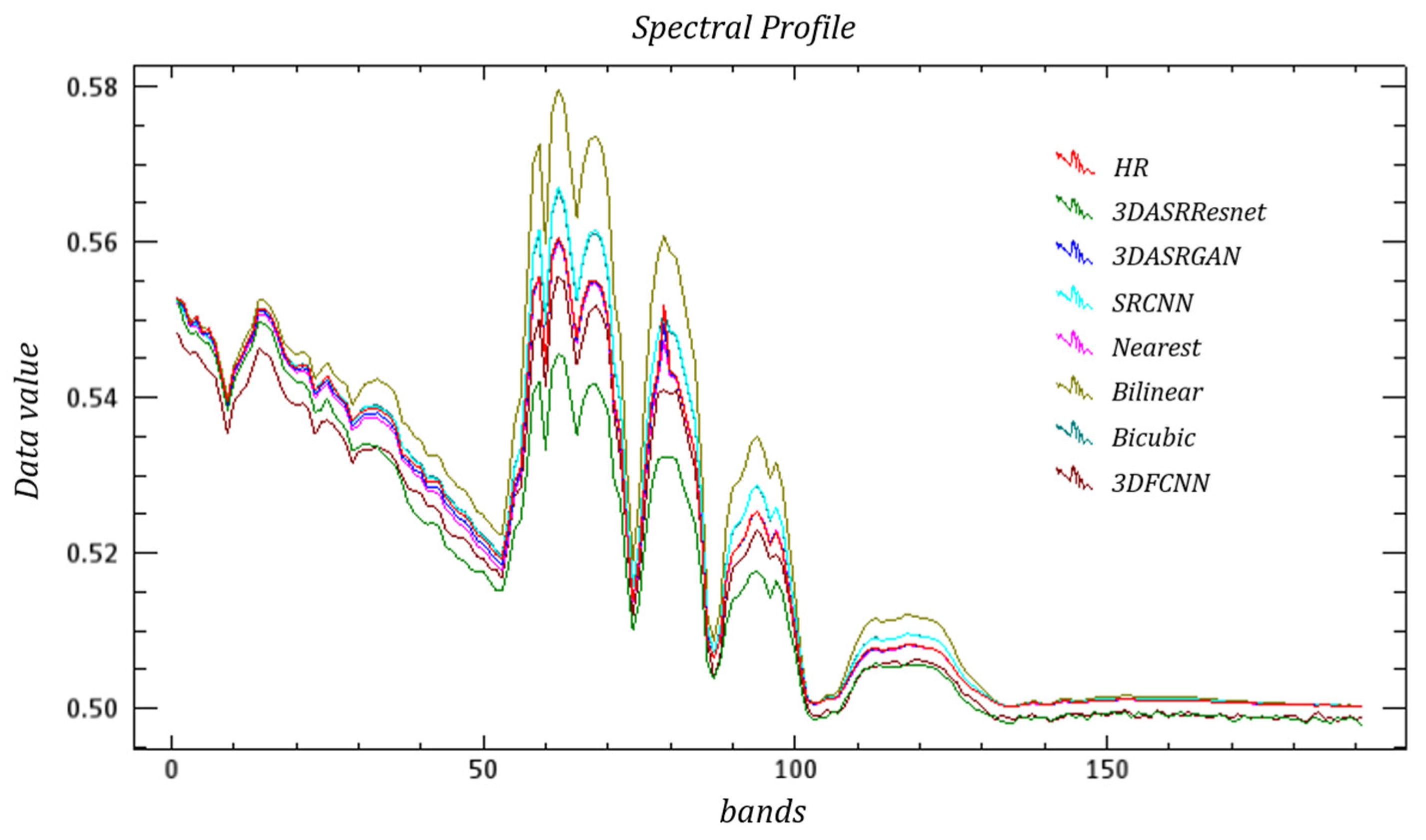
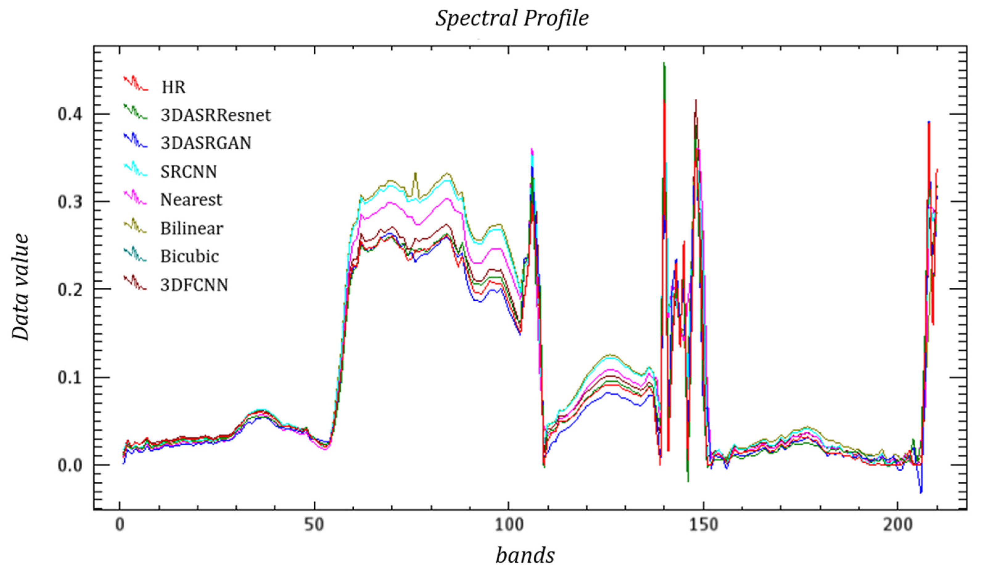
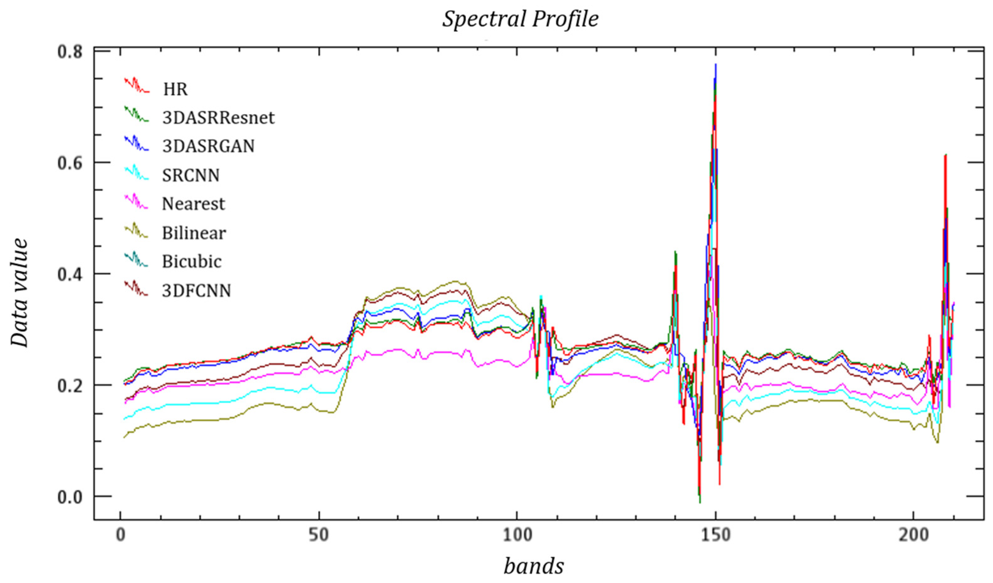
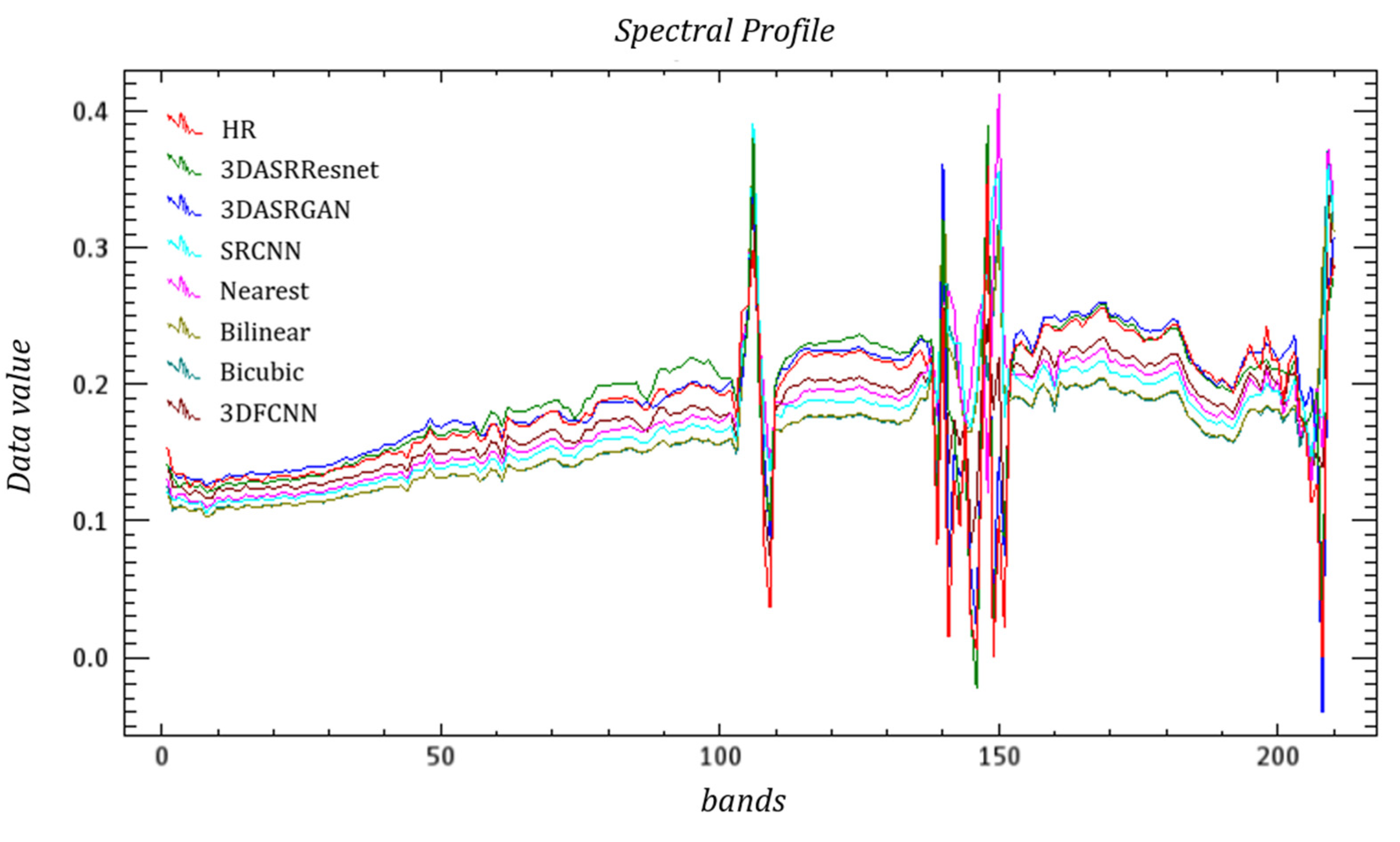
Figure 9, Figure 10 and Figure 11 and Figure 12, Figure 13 and Figure 14 present the spectral curves of several typical ground objects—grassland, roof, and road—after hyperspectral reconstruction, using various methods based on the two datasets. Overall, it can be observed from the positions of the peaks and valleys of the curves and the shapes of the curves that none of the seven methods produces a severe spectral distortion, and they are consistent with the spectral characteristic curves of the specific types of ground objects. However, when taking a closer look, we can see that the degree of deviation of the four curves varies. The red line represents the spectral curve from the HR image, which is the real image. The deep blue and green lines represent spectral curves from the proposed 3DASRGAN and 3DASRResNet, respectively. In Figure 9, Figure 10 and Figure 11, we can see that the red line is the closest to the deep blue line and the second-closest one is the green line, which means that the proposed 3DASRGAN model and 3DASRResNet model can create the most similar spectral information as real ground objects. For example, Figure 11 shows the spectral curves of roads based on the Washington DC Mall dataset. In the visible and near-infrared band, the spectral curves are quite different. It is seen that in the overall shape of each curve, the positions of the wave peak and valley are not quite different, which indicate that there is no serious deviation. The deep blue and green lines are closer to the red HR line, and their curves are relatively smooth and continuous. The next results, close to the red line, are that of 3D-FCNN and SRCNN. In contrast, the curves of bilinear, bicubic, and nearest methods show some irregular jitters, the overall curves are not smooth, and the differences are obvious.
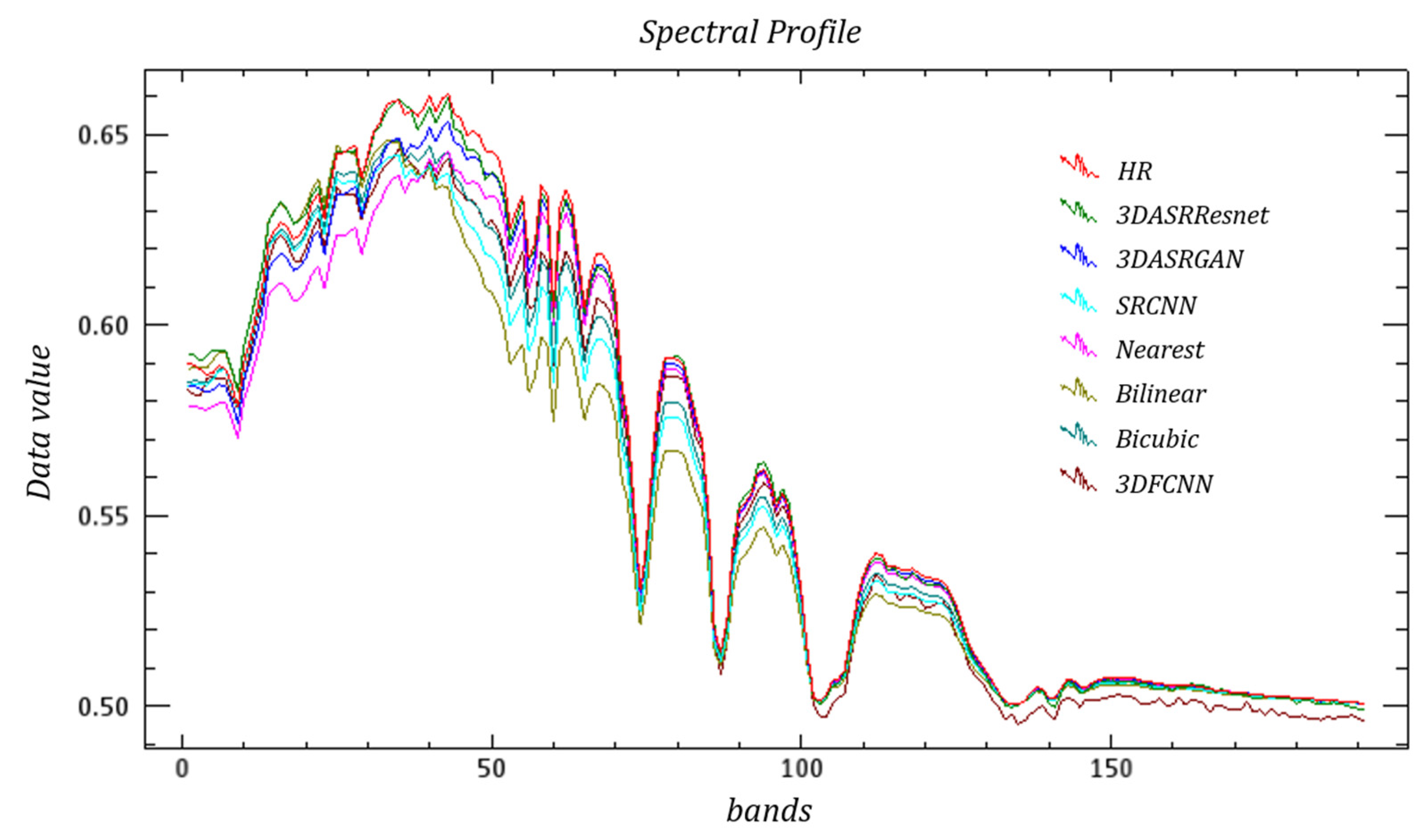
In Figure 12, Figure 13 and Figure 14, the red lines are closer to both the deep blue and green lines. Therefore, the results obtained from both the 3DASRResNet and 3DASRGAN are effective because 3DASRResNet has the smallest SAM value and 3DASRGAN has the highest PSNR and SSIM values. Compared with these two methods, the spectral curves of other methods are quite different from those of real ground objects. Thus, the impacts are not very good.
4.3. DASRGAN and the Original SRGAN
In this section, we applied our 3DASRGAN model and the original SRGAN model to the Washington DC Mall dataset. By comparing their results, it can be proven that 3DASRGAN can apply to the HSI SR problem better than the original SRGAN. In this comparative experiment, in order to adapt SRGAN to the training of hyperspectral data, we made the following improvements to the original SRGAN model: firstly, because the original SRGAN is designed for the SR of RGB color image which has a small number of bands, it is necessary to adjust the number of output channels of the related layers in the network structure. Secondly, in the composition of the original loss function, content loss is used to limit the detail difference between the reconstructed image and the original image, which can reflect the subjective visual feeling of the image to a certain extent. Content loss makes use of the preprocessed, well-known VGG (visual geometry group) network, which has been trained to fully extract the feature map of pictures. The calculation process of content loss is as follows: firstly, the generated image and the real image are put into the VGG19 network, respectively, and a certain layer of the feature map of the network is extracted from their results. Then, the feature map of the two constructs MSE, after that the content loss is generated. The process can be explained by the following formula:
where indicates the feature map obtained by j-th convolution network within the VGG19 network and and describe the dimensions of the feature maps.
This can be applied to the HSIs. In order to make the comparative test more convincing and effective, we kept such content loss in the training of the original SRGAN, and added two groups of comparative tests, to use the VGG network to construct content loss and to directly use MSE as content loss. The formula of MSE is the same as Equation (6). The experimental results are described in the following paragraphs.
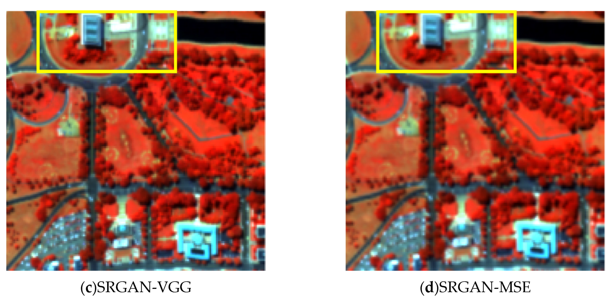
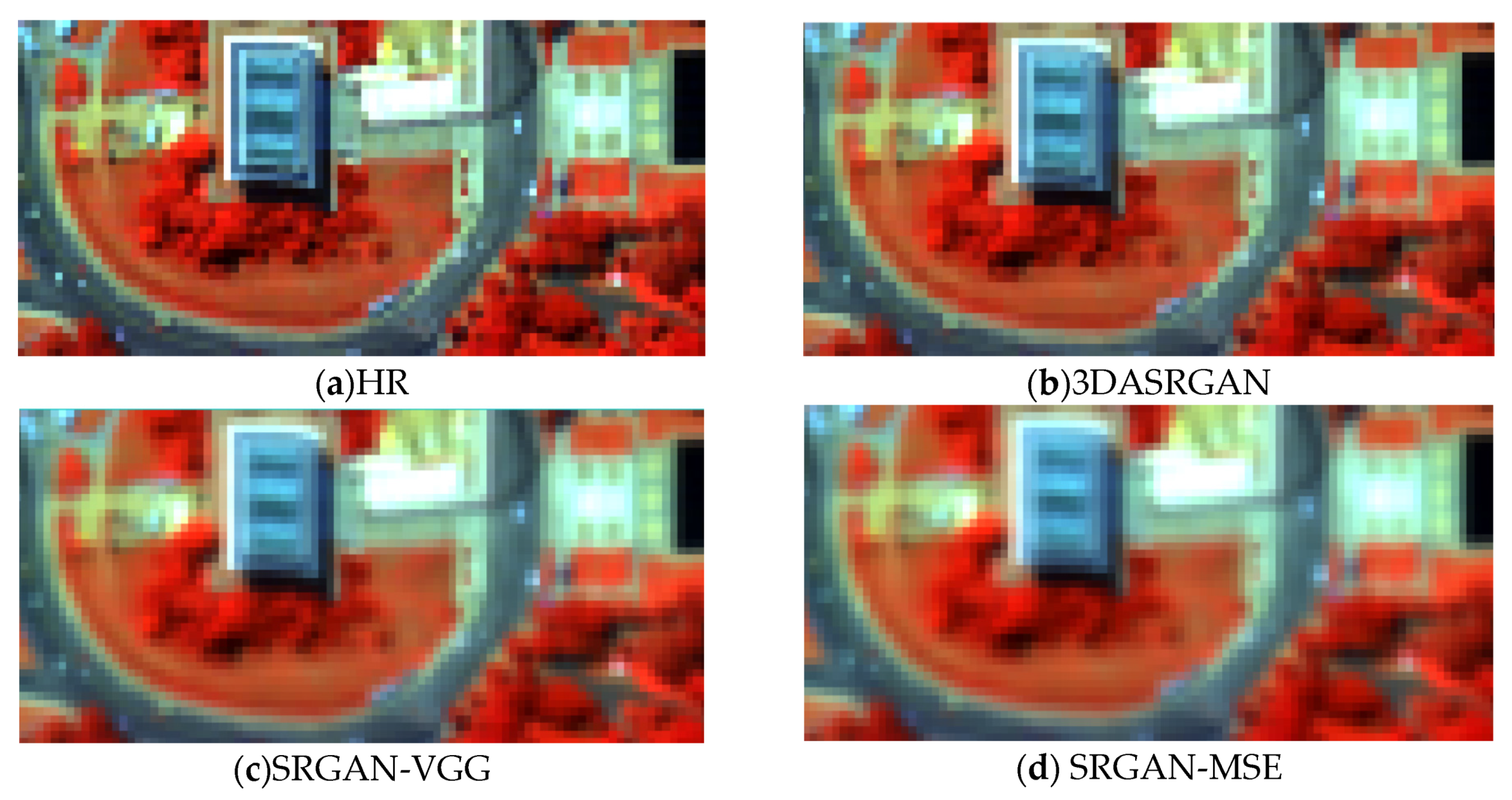
Figure 15 shows the results of 3DASRGAN, SRGAN-VGG, and SRGAN-MSE together with the HR image. From Figure 15c,d, we can see that the difference between SRGAN-VGG and SRGAN-MSE are not evident; the two results showed about the same blurring in the whole images. Compared with the results of SRGAN, the results of 3DASRGAN is a little clearer, but not significant. In order to better evaluate the effect of these methods, we chose a typical part to look at in detail, which is demonstrated in Figure 16.
In Figure 16, the difference of the 3DASRGAN and SRGAN methods are much clearer. Firstly, let us examine the results of SRGAN-VGG and SRGAN-MSE, which are shown in Figure 16c,d. In these results, the visual effect in 16c is slightly better than 16d, which is best illustrated by the shadows on the building’s roof and those of trees. However, the difference is not distinct. To some extent, this shows that the content loss constructed by VGG has no obvious effect on the HSI SR. The result of 3DASRGAN in 16b performs a little better and it is more similar to the HR image. The edges of the building are more distinct, the shadows of the trees and buildings are darker and more distinguishable. Spatial heterogeneity shows better in 3DASRGAN results. Nevertheless, the disparity between the results of 3DASRGAN and SRGAN have some difference in detail from the HR image. The similarity among SRGAN-VGG, SRGAN-MSE, and 3DASRGAN in the spatial aspect means that the space reconstruction ability of 3DASRGAN is better.
Table 3 shows the PSNR, SSIM, and SAM values of 3DASRGAN, SRGAN-VGG, SRGAN-MSE, and the HR image; our focus is the SAM value, which indicates the disparity of these methods. The SAM values of SRGAN-VGG and SRGAN-MSE are approximately the same, and they are both too high, which means that the spectral restoration ability of VGG and MSE methods are both ineffective and the spectral distortion of these two methods are obvious. Compared to the SRGAN methods, the SAM value of 3DASRGAN method is much closer to 0. The smaller SAM value shows the spectral curves of 3DASRGAN are more similar to the HR image, and thus, proves a better spectral reconstruction ability.
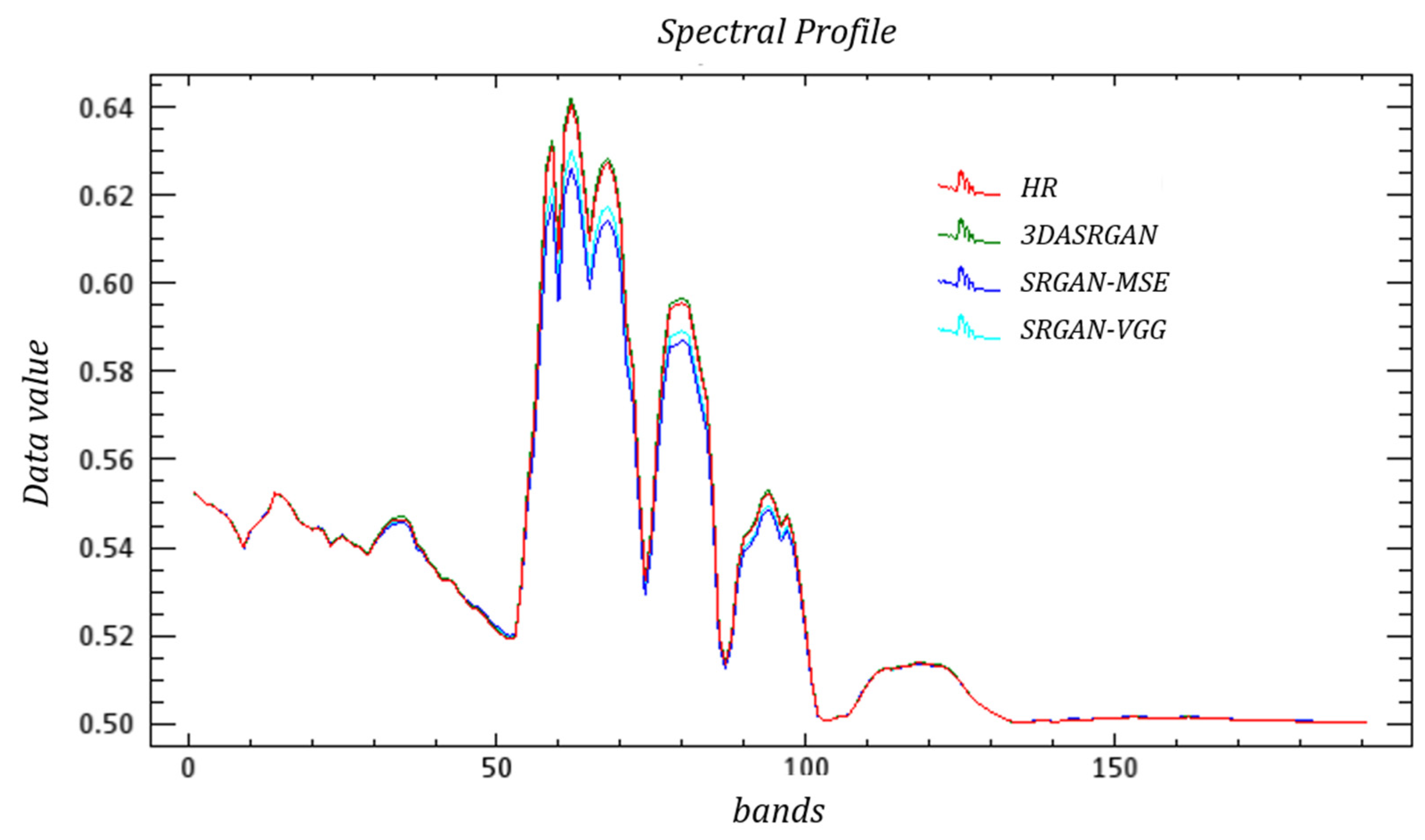
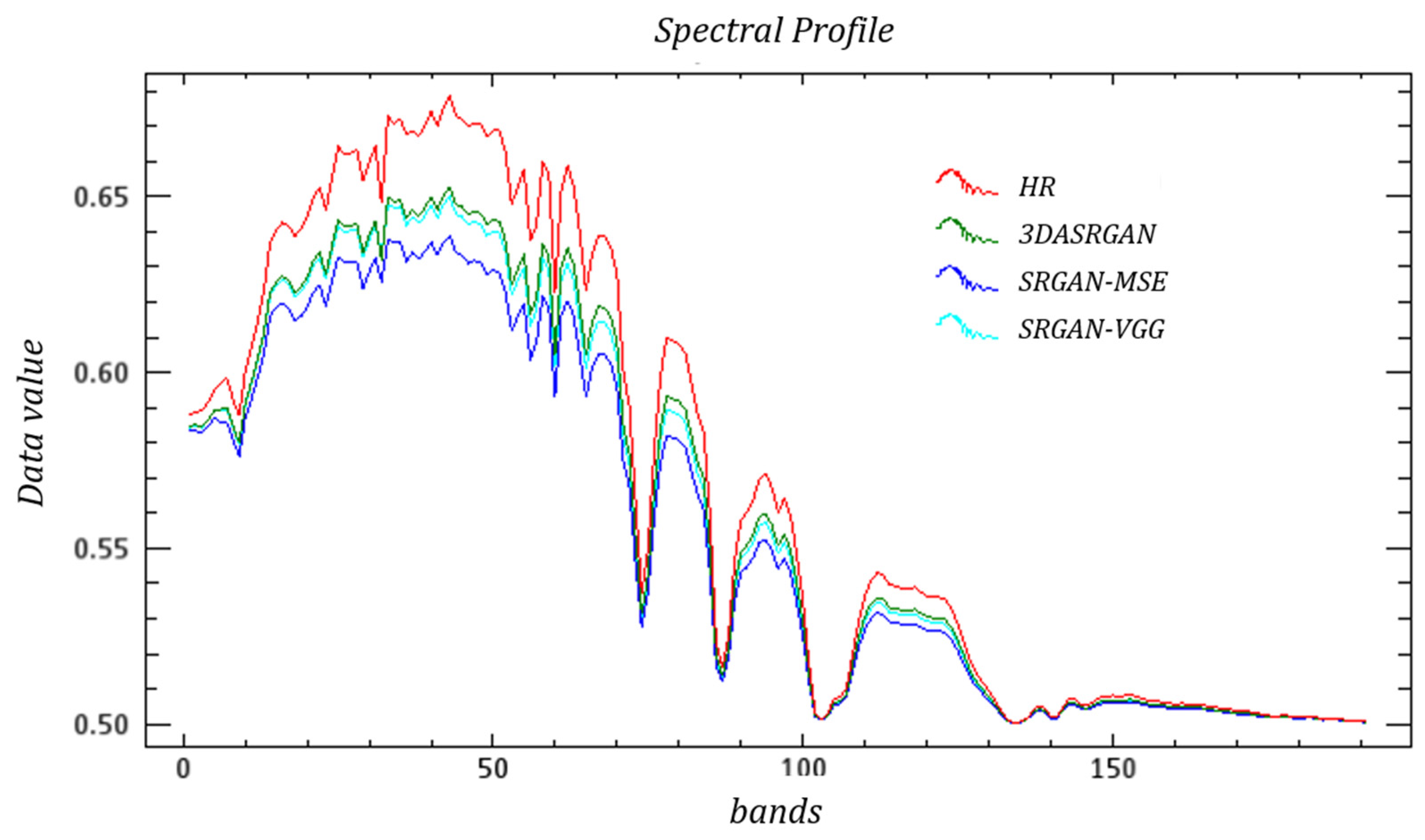
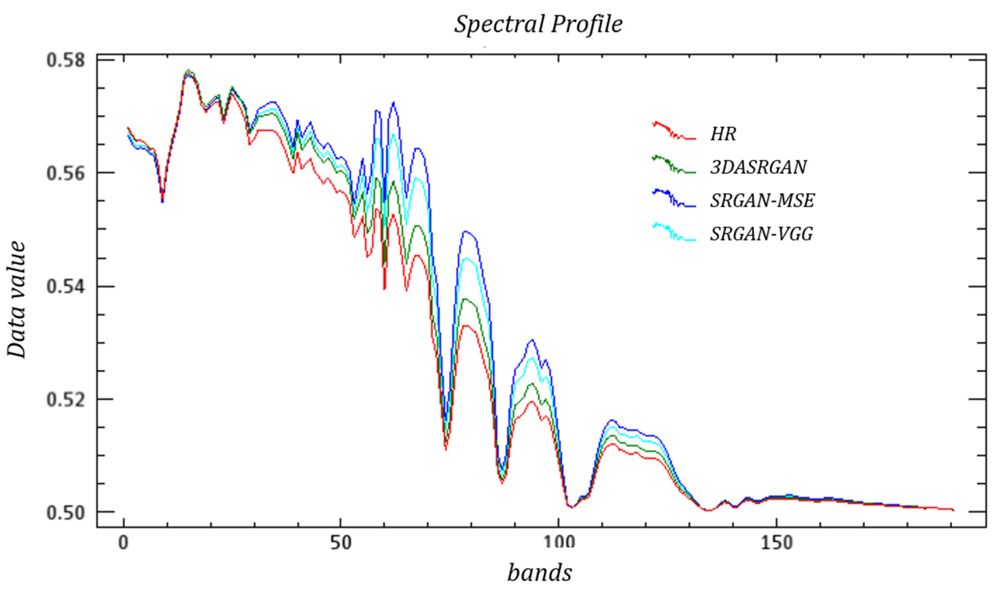
Meanwhile, Figure 17, Figure 18 and Figure 19 show the spectral curves of different objects. In general, both 3DASRGAN and the original SRGAN have many similarities with the HR; however, after close observation, for example the curves of grass, which show some difference at bands 1–10 and 40–50, the 3DASRGAN’s curve has almost uniform tendency with the HR’s. Contrastingly, the other two original SRGAN’s curves present a lower angle and a steeper slope than HS’s, while missing a local peak around the band 55. The same circumstance also occurs in the figure of the roof curves; it shows a lot of discordance at the band 30–50, with some notable malposition of peak and trough.
4.4. Discussion
In general, the 3DASRGAN is proposed to learn an end-to-end full-band mapping between low and high spatial-resolution HSIs. It makes full use of 3D convolution to fully extract the features between wavebands of HSIs. While ensuring the reconstruction effect on the spatial dimension, a 3D convolutional network can also improve the spectral approximation between the reconstructed image and the original image, which has little possibilities to cause problems such as spectral distortion. Compared with other super resolution reconstruction methods, it has a relatively small SAM value. Additionally, the method makes use of the characteristics of GAN framework. By generating an adversarial network, it can further reduce the difference between the generated image and the original image. Moreover, it is a sensor-specific task; thus, it can do the fine-tuning and expand the use.
According to previous experiments, 3DASRGAN achieves a great result in both spatial aspect and spectral aspect, while other methods such as CNN and the original SRGAN cannot take both aspects into account simultaneously. The result of 3DASRGAN has the lowest SAM, and according to Figure 9, Figure 10, Figure 11, Figure 12, Figure 13 and Figure 14, the impact of spatial reconstruction is much more excellent. The original SRGAN could not achieve a good result when it is directly applied to the HSIs mostly because it is mainly designed for RGB images, but it also could reach a fine result in some ways. However, since the 3DASRGAN is based on the 3D convolution, the number of kernels used in it is much more than those used in the original SGRAN. Moreover, the computation of the 3D convolution is more complex and heavier, thus, it will spend much more time on training 3DASRGAN than on the original SRGAN and other 2D-convolution-based methods like SRCNN. The 3D-FCNN model also uses the 3D convolution layers but with fewer number of layers and kernels; thus, when training 3D-FCNN in the experiment, it takes less time than 3DASRGAN. In Table 4, we conclude the average time that different machine-learning-based methods use in training and testing.
Due to the complexity of the network, there is also some obvious differences in the memory that different methods used to store the parameters of a model. It is also a fundamental factor that limits the speed of training and testing. Table 5 also presents the memory that the parameters of different methods occupies (the GAN network only includes the generator part).
5. Conclusions
In this study, we proposed a 3DASRGAN model for SR of HSIs by identifying the end-to-end full-band mapping between LR and HR HSIs. The 3D convolution layer is applied in the SRAGAN network instead of 2D convolution layer, which explored both the spatial information in adjacent pixels together with the spectral correlation in adjacent bands. For better using the multiply features generated by the 3D convolution layers, we proposed the feature attention mechanism to weighting the features to expect the network can focus on those really matter for the SR task. Moreover, we altered the G loss by adding spectral loss to it; thus, the generator will trend to recover the band information more for HSIs SR.
Currently, the studies about 3D convolutional layers and channel attention mechanisms have done a lot of works regarding the SR problem and GAN, though there are still problems unsolved like the scale problem of SR and so on. We are certain this study can inspire the explorations in the further studies about SR problem of HSIs.
6. Support Materials
6.1. GAN and SRGAN
The GAN framework developed by Goodfellow et al. [29] has remarkably improved the learning ability of many networks. GAN is an adversarial generation model architecture that consists of two parts: a generator (G) and a discriminator (D). The task of G is to learn the real distribution from the input data and that of D is to distinguish whether the sample created by G is the real HR data or a generated one. The final goal of GAN is to let G learn the data distribution of the real HR image, which can be applied to LR images, by mutual gambling with D, which can be applied to LR images, and guarantee D to have a discrimination probability of 50% at the same time.
The development of the GAN framework provides a new approach to solve SR problem. In 2016, Ledig et al. [26] applied GAN to SR problems and formulated SRGAN model, which achieved excellent results. They identified the fact that most recent studies on SR use mean squared error (MSE) as loss function, which causes over-smoothening and thus the loss of high-frequency details. A perceptual loss is used in SRGAN to solve these problems, which is made up of adversarial loss and content loss. The objective of adversarial loss is ensuring realistic-looking output image with higher resolution generated by G that maintains the pixel space to resemble the LR version. The content loss is based on similarity in perception rather than similarity in pixels, making the generated HR image more visually appealing. Therefore, this method can solve the problem of unrealistic visual effects effectively.
6.2. GAN Applications
Although SRGAN has demonstrated the remarkable potential to solve the SR problem, there is still space for improvement. Several researchers are searching for means to enhance this structure to make it more effective. Wang et al. [33] made some changes to the original SRGAN and built a new model called ESRGAN. They removed the BN layer and employed residual scaling to improve the performance and realize lower initialization when training a deep network structure, and improved the D using the relativistic average GAN. In this way, the G can provide more realistic texture details. Finally, they used the VGG features before activation and, thus, enhancing the perceptual loss. At the same time, ESRGAN demonstrates better performance with improved visual effects and lower perceptual index.
Meanwhile, Tran et al. [34] proposed a new architecture that incorporated the component of the adversarial networks form the SRGAN and the multi-scale learning component from the multiple scale super-resolution networks (MSSRNet). They improved the convolution layer in SRGAN with dilated convolution modules, which was also used in MSSRNet, and their networks were capable to extract the features of the images in different scales and recovering smaller objects in the images. To enhance the impact and the stability of their networks, they used WGAN (Wasserstein GAN) [35], which improved the performance.
More recently, Zhang et al. [13] proposed a ranker SRGAN, which could optimize the generator by using indifferentiable perceptual metrics and it worked well. By augmenting the training dataset with the results of other SR methods, this method was able to combine the strengths of various SR methods and improved the performance. Moreover, this SR structure could generate diversified results from different rank datasets, perceptual metrics and loss combinations.
6.3. Two-Dimensional and Three-Dimensional Convolution
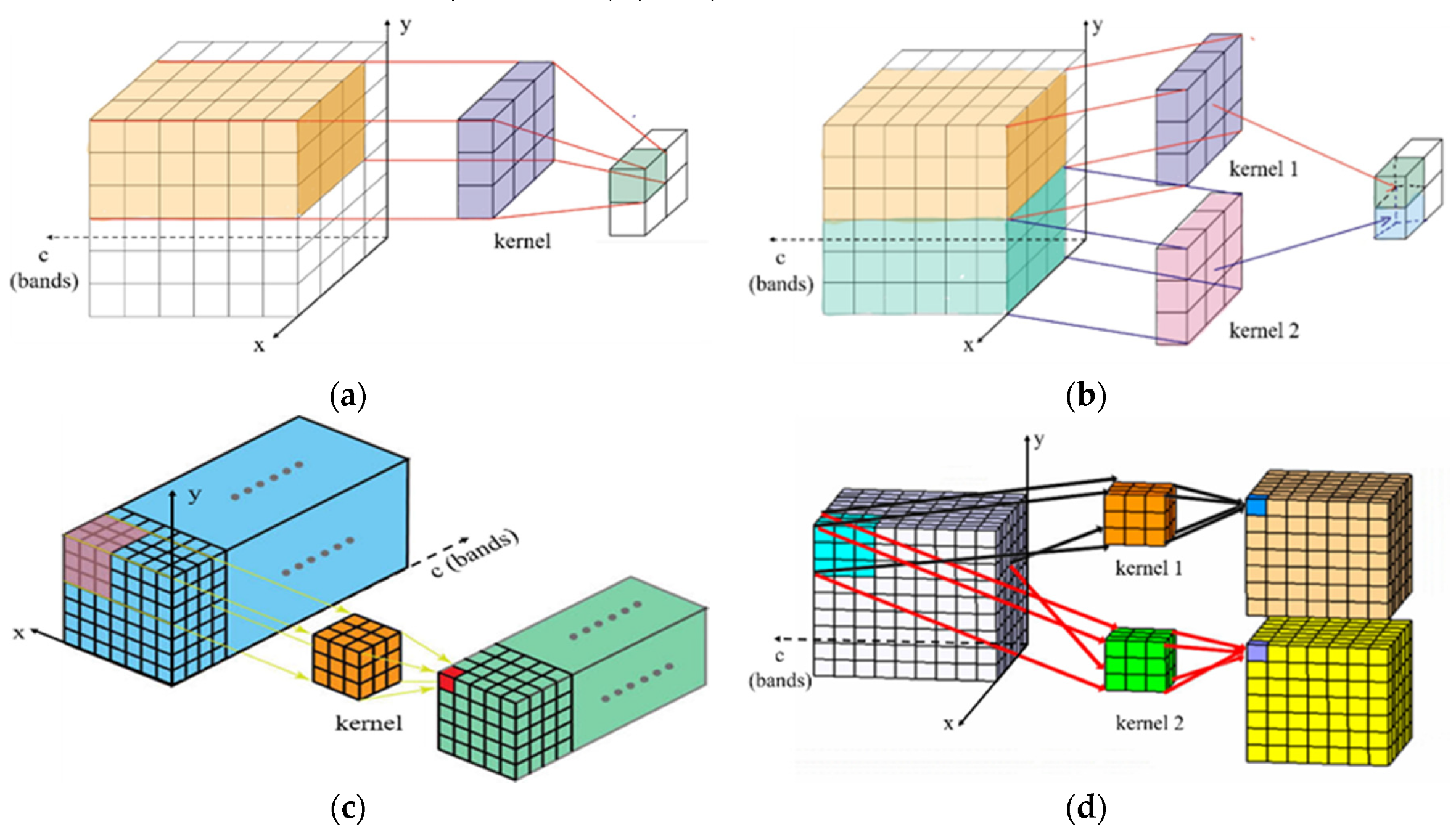
To extract the features in pixel level, 2D convolution uses a kernel to frame an extent and calculates the sum of the product of pixel and corresponding kernel value. The kernel is two-dimensional while the size of the kernel is flexible, depending on the size of the convolution. Every pixel value of the output of the 2D convolution is the sum of the product of kernel values and pixel values of the input. Figure 20a,b illustrates how a 2D convolution works. The convoluting process only occurs in the X and Y dimensions (the spatial dimensions), and the convoluted elements of the spectral dimension are summed together. If the kernel has the size of F × F, and the input image’s size is W × W, the stride is S, and the number of padding pixels is P, then the output size is reduced to N × N, in which N = (W − F + 2P)/(S + 1).
3D convolution, on the other hand, has a 3D kernel, which helps to achieve the convolution process to acquire features of the spatial as well as the spectral dimension. The main difference between 3D convolution and 2D convolution is that one more dimension is available for convolution in 3D convolution. 3D convolution is mainly used for video processing, when the convolution is applied to the frames of the video, it is also applied between these frames at the same time. Based on such characteristics, 3D convolution can simultaneously extract information along the spatial and spectral dimensions of HSIs. Figure 20c,d illustrates how a 3D convolution works by convoluting a 3D kernel with a cube formed by stacking multiple contiguous spectral bits of information together in both spatial and spectral dimensions. The size of each dimension of output N is calculated as N = (W − K + 2P)/(S + 1).
Either in 2D or 3D convolution, each convolution kernel is repeated on the whole image, and these repeated units share the same parameter settings including weight and bias, which is known as the weight sharing technique, and one kernel can extract the only feature of one kind from the entire data cube. To collect the various types of feature patterns, we normally use multiple 2D or 3D convolutions with various kernels in the network, as shown in Figure 20b–d.
In [25], Mei et al. also applied 3D convolution to the SR for HSIs. In their study, they expanded the size of LR using bicubic interpolation and then constructed an end to end 3D convolution network with four convolutional layers, where different numbers and sizes of kernels were used in different layers. In the end, the network was applied to the processed images; after the training process they could get a network for SR problem. Our network also contains 3D convolution, thus, it is meaningful to compare the impacts of both methods for solving the SR problem of HSIs.
Author Contributions
Conceptualization, Q.S.; Data curation, X.D. and Q.S.; Funding acquisition, M.L.; Methodology, X.D.; Software, X.D.; Supervision, Q.S.; Writing—review & editing, C.L., Q.S. and M.L. All authors have read and agreed to the published version of the manuscript.
Funding
This work is supported by Guangdong Natural Science Foundation (2019A1515011057), National Natural Science Foundation of China (61976234) and Open research fund of National Key Laboratory of surveying, mapping and remote sensing information engineering, Wuhan University 2.3
Conflicts of Interest
The authors declare no conflicts of interest.
References
- Yuan, Y.; Zheng, X.; Lu, X. Spectral-Spatial Kernel Regularized for Hyperspectral Image Denoising. IEEE Trans. Geosci. Remote Sens. 2015, 53, 3815–3832. [Google Scholar] [CrossRef]
- Nelson, M.P.; Shi, L.; Zbur, L.; Priore, R.J.; Treado, P.J. Real-Time Short-Wave Infrared Hyperspectral Conformal Imaging Sensor for the Detection of Threat Materials. In Chemical, Biological, Radiological, Nuclear, and Explosives; Fountain, A.W., Ed.; Spie Digital Library: Bellingham, WA, USA, 2016. [Google Scholar]
- Asadzadeh, S.; De Souza Filho, C.R. A review on spectral processing methods for geological remote sensing. Int. J. Appl. Earth Obs. Geoinf. 2016, 47, 69–90. [Google Scholar] [CrossRef]
- Xie, W.; Shi, Y.; Li, Y.; Jia, X.; Lei, J. High-quality spectral-spatial reconstruction using saliency detection and deep feature enhancement. Pattern Recognit. 2019, 88, 139–152. [Google Scholar] [CrossRef]
- Yuan, Y.; Zheng, X.; Lu, X. Hyperspectral Image Superresolution by Transfer Learning. IEEE J. Sel. Top. Appl. Earth Obs. Remote Sens. 2017, 10, 1963–1974. [Google Scholar] [CrossRef]
- Zhang, L.; Yuan, Q.; Shen, H.; Li, P. Multiframe image super-resolution adapted with local spatial information. J. Opt. Soc. Am. A-Opt. Image Sci. Vis. 2011, 28, 381–390. [Google Scholar] [CrossRef] [PubMed]
- Li, Y.; Hu, J.; Zhao, X.; Xie, W.; Li, J. Hyperspectral image super-resolution using deep convolutional neural network. Neurocomputing 2017, 266, 29–41. [Google Scholar] [CrossRef]
- Bungert, L.; Coomes, D.A.; Ehrhardt, M.J.; Rasch, J.; Reisenhofer, R.; Schönlieb, C.B. Blind image fusion for hyperspectral imaging with the directional total variation. Inverse Problems 2018, 34, 044003. [Google Scholar] [CrossRef]
- Yuan, Q.; Yan, L.; Li, J.; Zhang, L. Remote sensing image super-resolution via regional spatially adaptive total variation model. In Proceedings of the 2014 IEEE Geoscience and Remote Sensing Symposium, Quebec City, QC, Canada, 13–18 July 2014; pp. 3073–3076. [Google Scholar]
- Yuan, Q.; Zhang, L.; Shen, H. Regional Spatially Adaptive Total Variation Super-Resolution With Spatial Information Filtering and Clustering. IEEE Trans. Image Process. 2013, 22, 2327–2342. [Google Scholar] [CrossRef] [PubMed]
- Akhtar, N.; Shafait, F.; Mian, A. Bayesian Sparse Representation for Hyperspectral Image Super Resolution. In Proceedings of the 2015 IEEE Conference on Computer Vision and Pattern Recognition, Boston, MA, USA, 7–12 June 2015; pp. 3631–3640. [Google Scholar]
- Kawakami, R.; Matsushita, Y.; Wright, J.; Ben-Ezra, M.; Tai, Y.W.; Ikeuchi, K. High resolution Hyperspectral Imaging via Matrix Factorization. In Proceedings of the 2011 IEEE Conference on Computer Vision and Pattern Recognition, Colorado Springs, CO, USA, 20–25 June 2011. [Google Scholar]
- Dong, C.; Loy, C.C.; He, K.; Tang, X. Image Super-Resolution Using Deep Convolutional Networks. IEEE Trans. Pattern Anal. Mach. Intell. 2016, 38, 295–307. [Google Scholar] [CrossRef] [PubMed] [Green Version]
- Zhang, K.; Wang, M.; Yang, S.; Jiao, L. Spatial-Spectral-Graph. Regularized Low-Rank Tensor Decomposition for Multispectral and Hyperspectral Image Fusion. IEEE J. Sel. Top. Appl. Earth Obs. Remote Sens. 2018, 11, 1030–1040. [Google Scholar] [CrossRef]
- Li, S.; Dian, R.; Fang, L.; Bioucas-Dias, J.M. Fusing Hyperspectral and Multispectral Images via Coupled Sparse Tensor Factorization. IEEE Trans. Image Process. 2018, 27, 4118–4130. [Google Scholar]
- Wei, Y.; Yuan, Q.; Shen, H.; Zhang, L. A Universal Remote Sensing Image Quality Improvement Method with Deep Learning. In Proceedings of the 2016 IEEE International Geoscience and Remote Sensing Symposium, Beijing, China, 10–15 July 2016; pp. 6950–6953. [Google Scholar]
- Wei, Y.; Yuan, Q. Deep Residual Learning for Remote Sensed Imagery Pansharpening. In Proceedings of the 2017 International Workshop on Remote Sensing with Intelligent Processing, Shanghai, China, 19–21 May 2017. [Google Scholar]
- Zhang, L.; Shen, H.; Gong, W.; Zhang, H. Adjustable Model. Based Fusion Method for Multispectral and Panchromatic Images. IEEE Trans. Syst. Man Cybern. Part B Cybern. 2012, 42, 1693–1704. [Google Scholar]
- Shen, H.; Jiang, M.; Li, J.; Yuan, Q.; Wei, Y.; Zhang, L. Spatial-Spectral Fusion by Combining Deep Learning and Variational Model. IEEE Trans. Geosci. Remote Sens. 2019, 57, 6169–6181. [Google Scholar] [CrossRef]
- Zhang, L.; Zhang, L.; Du, B. Deep Learning for Remote Sensing Data A technical tutorial on the state of the art. IEEE Geosci. Remote Sens. Mag. 2016, 4, 22–40. [Google Scholar] [CrossRef]
- Kim, J.; Kwon Lee, J.; Mu Lee, K. Accurate Image Super-Resolution Using Very Deep Convolutional Networks. In Proceedings of the 2016 IEEE Conference on Computer Vision and Pattern Recognition, Las Vegas, NV, USA, 27–30 June 2016; pp. 1646–1654. [Google Scholar]
- Simonyan, K.; Zisserman, A. Very Deep Convolutional Networks for Large-Scale Image Recognition. arXiv 2014, arXiv:1409.1556. [Google Scholar]
- Dong, C.; Loy, C.C.; Tang, X. Accelerating the Super-Resolution Convolutional Neural Network. In Computer Vision-Eccv 2016; Li, P., Leibe, B., Eds.; Springer International Publishing: New York, NY, USA, 2016; pp. 391–407. [Google Scholar]
- Kim, J.; Kwon Lee, J.; Mu Lee, K. Deeply-Recursive Convolutional Network for Image Super-Resolution. In Proceedings of the 2016 IEEE Conference on Computer Vision and Pattern Recognition, Las Vegas, NV, USA, 27–30 June 2016; pp. 1637–1645. [Google Scholar]
- He, K.; Zhang, X.; Ren, S.; Sun, J. Real-Time Single Image and Video Super-Resolution Using an Efficient Sub-Pixel Convolutional Neural Network. In Proceedings of the 2016 IEEE Conference on Computer Vision and Pattern Recognition, Vision and Pattern Recognition, Las Vegas, NV, USA, 27–30 June 2016; pp. 1874–1883. [Google Scholar]
- Han, X.H.; Shi, B.; Zheng, Y. SSF-CNN: SPATIAL AND SPECTRAL FUSION WITH CNN FOR HYPERSPECTRAL IMAGE SUPER-RESOLUTION. In Proceedings of the 2018 25th IEEE International Conference on Image Processing, Athens, Greece, 7–10 October 2018; pp. 2506–2510. [Google Scholar]
- Luo, Y.; Zou, J.; Yao, C.; Zhao, X.; Li, T.; Bai, G. HSI-CNN: A Novel Convolution Neural Network for Hyperspectral Image. In Proceedings of the 2018 International Conference on Audio, Language and Image Processing, Shanghai, China, 16–17 July 2018; pp. 464–469. [Google Scholar]
- Mei, S.; Yuan, X.; Ji, J.; Zhang, Y.; Wan, S.; Du, Q. Hyperspectral Image Spatial Super-Resolution via 3D Full Convolutional Neural Network. Remote Sens. 2017, 9, 1139. [Google Scholar] [CrossRef] [Green Version]
- Ghahramani, Z. Generative Adversarial Nets. In Advances in Neural Information Processing Systems 27; Ghahramani, Z. Neural Information Processing Systems Inc.: Vancouver, BC, Canada, 2014. [Google Scholar]
- Ledig, C.; Theis, L.; Huszár, F.; Caballero, J.; Cunningham, A.; Acosta, A.; Shi, W. Photo-Realistic Single Image Super-Resolution Using a Generative Adversarial Network. In Proceedings of the 30th IEEE Conference on Computer Vision and Pattern Recognition, Honolulu, HI, USA, 21–26 July 2017; pp. 105–114. [Google Scholar]
- Bock, S.; Weiß, M.; Goppold, J. An improvement of the convergence proof of the ADAM-Optimizer. 2018. Available online: http://arxiv.org/abs/1804.10587 (accessed on 1 January 2020).
- Wang, Z.; Bovik, A.C.; Sheikh, H.R.; Simoncelli, E.P. Image quality assessment: From error visibility to structural similarity. IEEE Trans. Image Process. 2004, 13, 600–612. [Google Scholar] [CrossRef] [PubMed] [Green Version]
- Wang, X.; Yu, K.; Wu, S.; Gu, J.; Liu, Y.; Dong, C.; Qiao, Y.; Loy, C.C. Esrgan: Enhanced super-resolution generative adversarial networks. In ECCV 2018: Computer Vision–ECCV 2018 Workshops, Proceedings of European Conference on Computer Vision, Munich, Germany, 8–14 September 2018; Leal-Taixé, L., Roth, S., Eds.; Springer: Berlin, Germany, 2018; pp. 63–79. [Google Scholar]
- Tran, K.; Panahi, A.; Adiga, A.; Sakla, W.; Krim, H. Nolinear Multi-scalw Super-resolution using deep learning. In Proceedings of the 2019 IEEE International Conference on Acoustics, Speech and Signal. Processing, Brighton, UK, 12–17 May 2019; pp. 3182–3186. [Google Scholar]
- Arjovsky, M.; Chintala, S.; Bottou, L. Wasserstein GAN. arXiv 2017, arXiv:1701.07875, 30. [Google Scholar]
Figure 1.
The architecture of generator (a) and discriminator (b) networks with the corresponding number of ResNet blocks (K), number of feature maps (n), and stride (s) are indicated for each convolutional layer.
Figure 1.
The architecture of generator (a) and discriminator (b) networks with the corresponding number of ResNet blocks (K), number of feature maps (n), and stride (s) are indicated for each convolutional layer.

Figure 2.
The Architecture of the Employed Attention Strategy. In general, the feature attention mechanism we proposed includes one average-pooling layers, two thin fully connected networks (FC layers), and a multiply operation of the scaling coefficient and the input tensor.
Figure 2.
The Architecture of the Employed Attention Strategy. In general, the feature attention mechanism we proposed includes one average-pooling layers, two thin fully connected networks (FC layers), and a multiply operation of the scaling coefficient and the input tensor.

Figure 3.
The framework of proposed three-dimensional Attention-based Super-Resolution Generative Adversarial Network (3DASRGAN) for SR of hyperspectral remote sensing images (HSIs).
Figure 3.
The framework of proposed three-dimensional Attention-based Super-Resolution Generative Adversarial Network (3DASRGAN) for SR of hyperspectral remote sensing images (HSIs).

Figure 4.
The Map of the Composition Structure of Training and Testing Data.

Figure 5.
Results of various SR HSI methods and original low-resolution (LR) and high-resolution (HR) images based on Washington DC Mall dataset.
Figure 5.
Results of various SR HSI methods and original low-resolution (LR) and high-resolution (HR) images based on Washington DC Mall dataset.

Figure 6.
Image parts of different SR HSI methods and original LR and HR images based on Washington DC Mall dataset
Figure 6.
Image parts of different SR HSI methods and original LR and HR images based on Washington DC Mall dataset


Figure 7.
Results obtained from various SR HSI methods and Original LR and HR images based on the Urban dataset.
Figure 7.
Results obtained from various SR HSI methods and Original LR and HR images based on the Urban dataset.

Figure 8.
Image parts produced by various SR HSI methods and original LR and HR images based on the Urban dataset.
Figure 8.
Image parts produced by various SR HSI methods and original LR and HR images based on the Urban dataset.


Figure 9.
Example Spectral Curves of Grass based on Washington DC Mall dataset.

Figure 10.
Example Spectral Curves of Roof based on Washington DC Mall dataset.

Figure 11.
Example Spectral Curves of Roads based on the Washington DC Mall dataset.

Figure 12.
Example Spectral Curves of Grass based on the Urban dataset.

Figure 13.
Example Spectral Curves of Roof based on the Urban dataset.

Figure 14.
Example Spectral Curves of Road based on the Urban dataset.

Figure 15.
Results of the HR image, 3DASRGAN, SRGAN-VGG, and SRGAN-MSE based on the Washington DC Mall dataset.
Figure 15.
Results of the HR image, 3DASRGAN, SRGAN-VGG, and SRGAN-MSE based on the Washington DC Mall dataset.


Figure 16.
Details of the results of the HR image, 3DASRGAN, SRGAN-VGG, and SRGAN-MSE based on the Washington DC Mall dataset.
Figure 16.
Details of the results of the HR image, 3DASRGAN, SRGAN-VGG, and SRGAN-MSE based on the Washington DC Mall dataset.

Figure 17.
Example Spectral Curves of Grass based on the Washington DC Mall dataset.

Figure 18.
Example Spectral Curves of Roof based on the Washington DC Mall dataset.

Figure 19.
Example Spectral Curves of Road based on the Washington DC Mall dataset.

Figure 20.
The difference between two-dimensional (2D) convolution and three-dimensional (3D) convolution; (a) 2D convolution extracted features; (b) 2D convolution with multiply kernels; (c) 3D convolution extracted features; (d) 3D convolution with multiply kernels.
Figure 20.
The difference between two-dimensional (2D) convolution and three-dimensional (3D) convolution; (a) 2D convolution extracted features; (b) 2D convolution with multiply kernels; (c) 3D convolution extracted features; (d) 3D convolution with multiply kernels.


Table 1.
Quantitative comparison results of different SR methods based on the Washington DC Mall dataset.
Table 1.
Quantitative comparison results of different SR methods based on the Washington DC Mall dataset.
| PSNR | SSIM | SAM | |
|---|---|---|---|
| 3DASRResNet | 31.0576 | 0.966 | 5.203 |
| 3DASRGAN | 32.2701 | 0.971 | 5.269 |
| 3D-FCNN | 29.5369 | 0.966 | 5.216 |
| SRCNN | 28.7258 | 0.942 | 5.866 |
| Bicubic | 27.8104 | 0.937 | 6.683 |
| Bilinear | 28.4136 | 0.861 | 10.514 |
| Nearest | 27.2407 | 0.725 | 22.759 |
| HR | ∞ | 1 | 0 |
Table 2.
Quantitative comparison results of different SR methods based on the Urban dataset.
| PSNR | SSIM | SAM | |
|---|---|---|---|
| 3DASRResNet | 30.1022 | 0.908 | 2.838 |
| 3DASRGAN | 33.2755 | 0.911 | 2.694 |
| 3D-FCNN | 30.4639 | 0.901 | 3.074 |
| SRCNN | 28.0737 | 0.916 | 3.717 |
| Bicubic | 28.5427 | 0.866 | 4.552 |
| Bilinear | 27.1950 | 0.781 | 6.798 |
| Nearest | 27.0478 | 0.702 | 15.179 |
| HR | ∞ | 1 | 0 |
Table 3.
Quantitative comparison results of 3DASRGAN and SRGAN based on the Washington DC Mall dataset.
Table 3.
Quantitative comparison results of 3DASRGAN and SRGAN based on the Washington DC Mall dataset.
| PSNR | SSIM | SAM | |
|---|---|---|---|
| 3DASRGAN | 32.2701 | 0.971 | 5.269 |
| SRGAN-MSE | 28.3744 | 0.952 | 5.583 |
| SRGAN-VGG | 28.5017 | 0.966 | 5.470 |
| HR | ∞ | 1 | 0 |
Table 4.
The occupied memories of different SR methods on the Washington DC Mall dataset.
| Parameters Memories | |
|---|---|
| 3DASRGAN | 118.37M |
| SRGAN | 46.32M |
| 3D-FCNN | 39.40M |
| SRCNN | 12.27M |
Table 5.
The computation time of different SR methods on the Washington DC Mall dataset.
| Training | Test | |
|---|---|---|
| 3DASRGAN | 26h | 5s |
| SRGAN-MSE | 16h | 3s |
| SRGAN-VGG | 16h | 3s |
| 3D-FCNN | 20h | 3s |
| SRCNN | 6h | 2s |
© 2020 by the authors. Licensee MDPI, Basel, Switzerland. This article is an open access article distributed under the terms and conditions of the Creative Commons Attribution (CC BY) license (http://creativecommons.org/licenses/by/4.0/).
Share and Cite
MDPI and ACS Style
Dou, X.; Li, C.; Shi, Q.; Liu, M. Super-Resolution for Hyperspectral Remote Sensing Images Based on the 3D Attention-SRGAN Network. Remote Sens. 2020, 12, 1204. https://0-doi-org.brum.beds.ac.uk/10.3390/rs12071204
AMA Style
Dou X, Li C, Shi Q, Liu M. Super-Resolution for Hyperspectral Remote Sensing Images Based on the 3D Attention-SRGAN Network. Remote Sensing. 2020; 12(7):1204. https://0-doi-org.brum.beds.ac.uk/10.3390/rs12071204
Chicago/Turabian StyleDou, Xinyu, Chenyu Li, Qian Shi, and Mengxi Liu. 2020. "Super-Resolution for Hyperspectral Remote Sensing Images Based on the 3D Attention-SRGAN Network" Remote Sensing 12, no. 7: 1204. https://0-doi-org.brum.beds.ac.uk/10.3390/rs12071204
Note that from the first issue of 2016, this journal uses article numbers instead of page numbers. See further details here.