Satellite Observations for Detecting and Forecasting Sea-Ice Conditions: A Summary of Advances Made in the SPICES Project by the EU’s Horizon 2020 Programme

 ,
,  , ,
, ,  , , , , , ,
  and
and 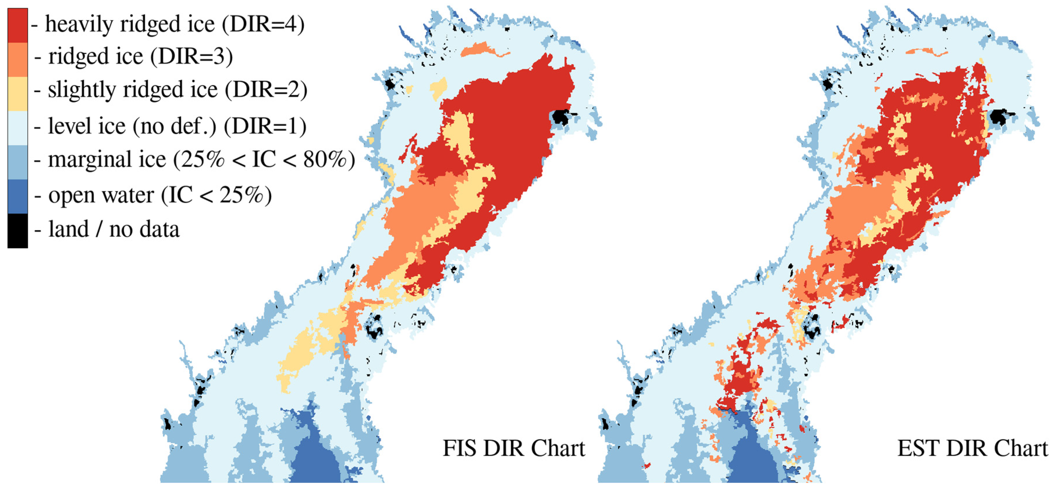
Abstract
:1. Introduction
2. New Products of Sea-Ice Conditions
2.1. Degree of Sea-Ice Ridging Using Synthetic Aperture Radar (SAR)
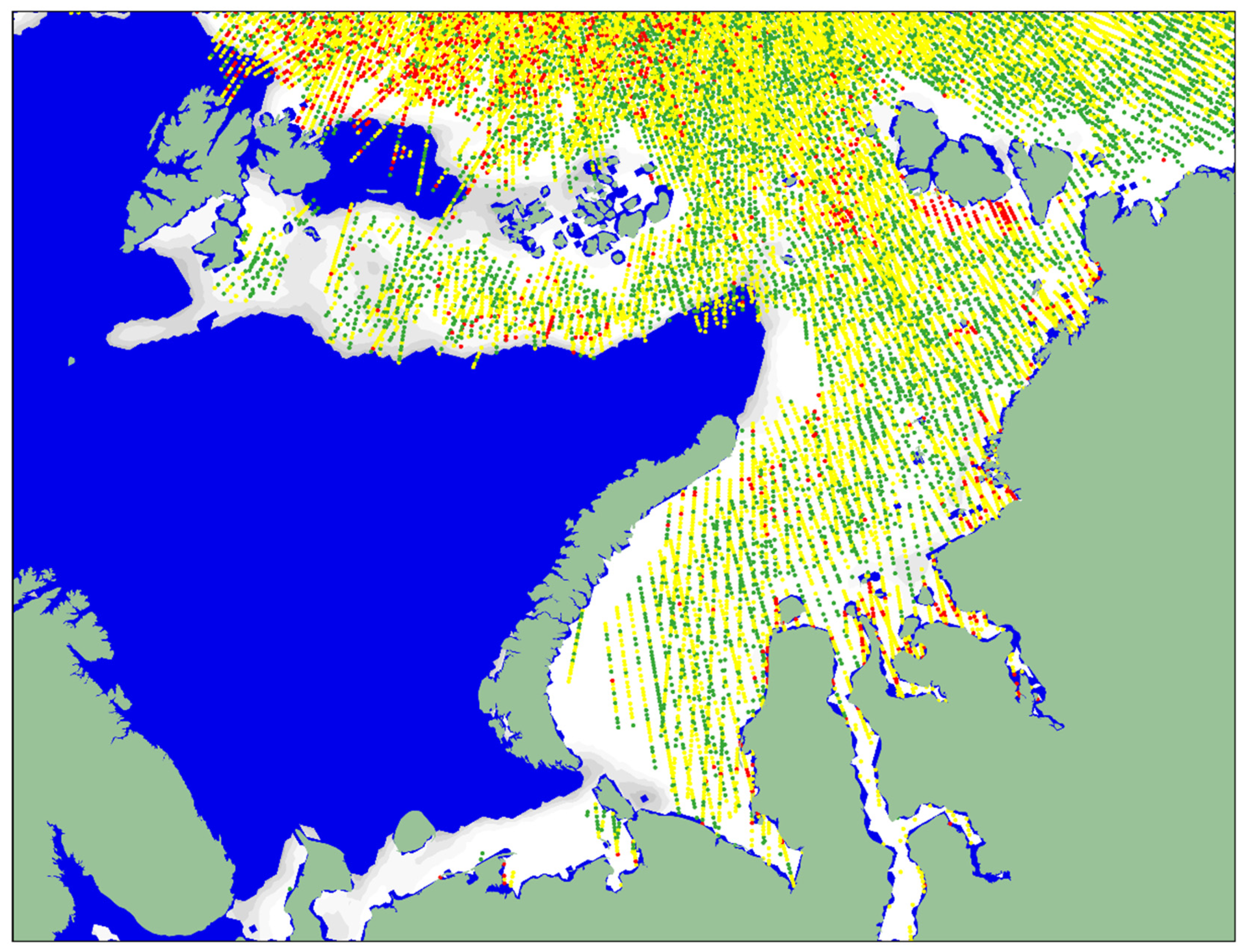
2.2. Determination of Pancake Ice Thickness Using SAR
2.3. Determination of Risk Index Outcome (RIO) of International Maritime Organization (IMO) Polar Code with CryoSat-2 SAR Interferometer Radar Altimeter (SIRAL) Data
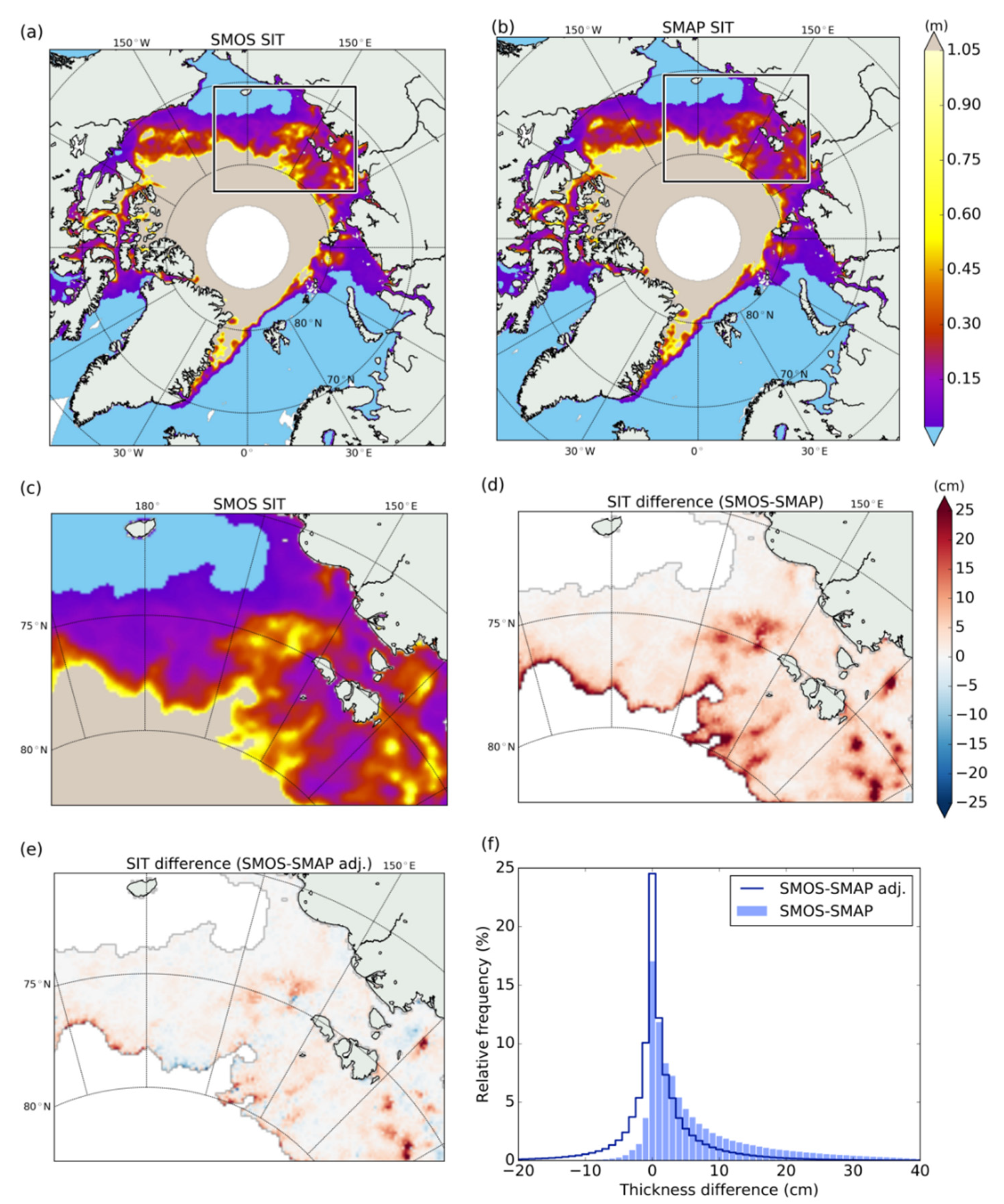
2.4. Thin Ice Thickness from Combined Soil Moisture and Ocean Salinity (SMOS) and Soil Moisture Active Passive (SMAP) Data
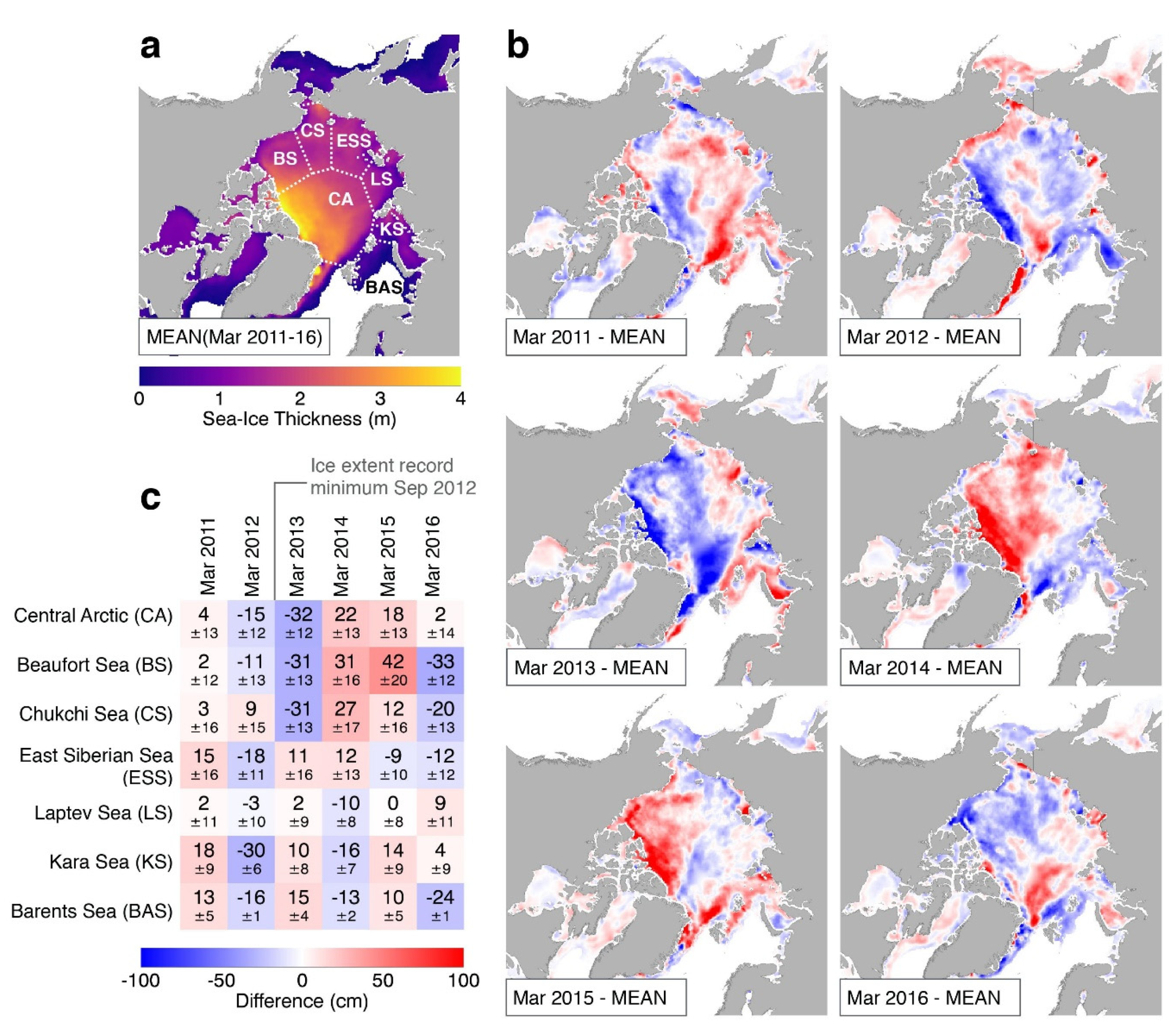
2.5. Sea-Ice Drift, Thickness and Volume Fluxes Estimation Using Multi-Sensor Satellite Data
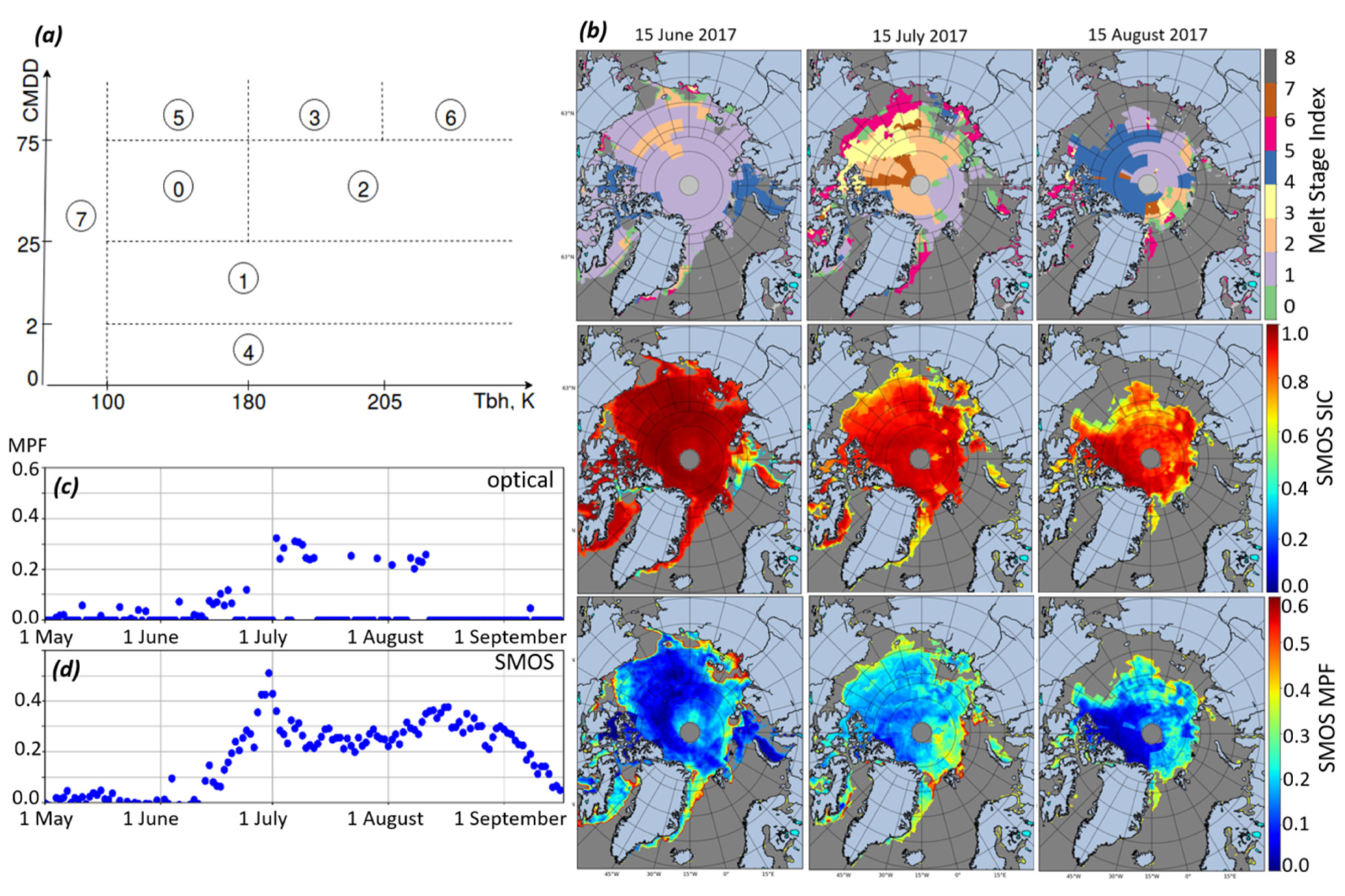
2.6. Melt Pond Fraction, Melt Stage, and Sea-Ice Concentration Using SMOS Data
- Sea-ice disintegration after short melt period, end phase of thin ice melt: high water content inside ice, high open water fraction, ponds melt through, high MPF.
- Melt onset (if CMDD = 0 all the time before): water content inside ice is low, low lateral melt, surface MPF increases; or melt after cold spell (if CMDD was positive before): water content in ice high, high lateral melt, MPF potentially high.
- Stable melt on dense sea ice: water content within ice low, moderate lateral melt, MPF is the main cause of change.
- Stable melt after second MPF peak on porous ice: water content within sea ice higher, moderate lateral melt, MPF moderate high.
- Freeze up or cold spell during summer: most ponds frozen over, ocean assumed open, brine or ocean water within ice present as before.
- End stage of longer melt: water content in ice high, very strong lateral melt, high surface melt.
- MYI or drastic melt onset: water content within sea ice low, low lateral melt, reacts to mostly MPF.
- Open water: ocean or polynya.
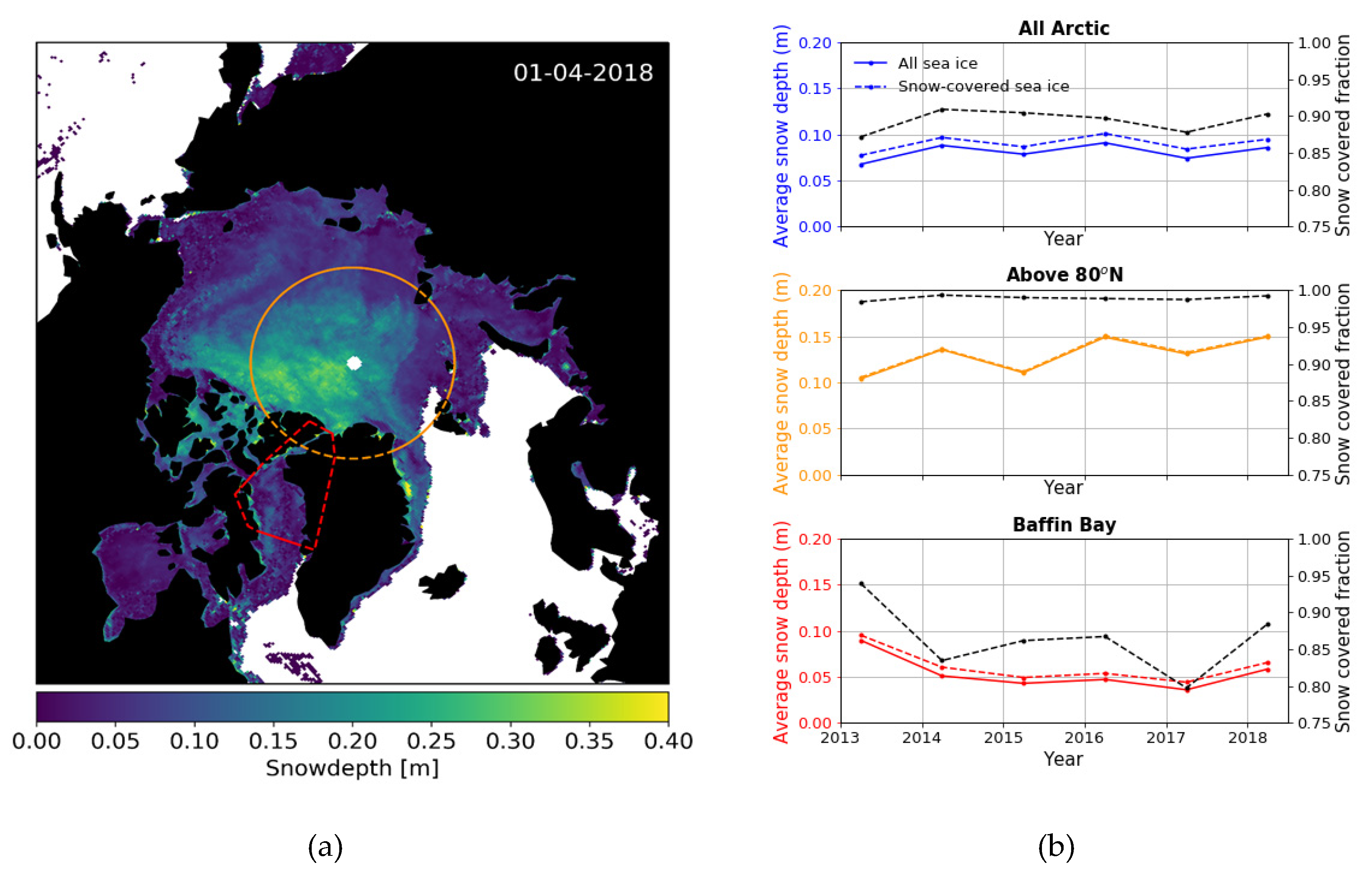
2.7. Snow Depth on Sea Ice Using Microwave Radiometer (MR) Data and Optimal Estimation
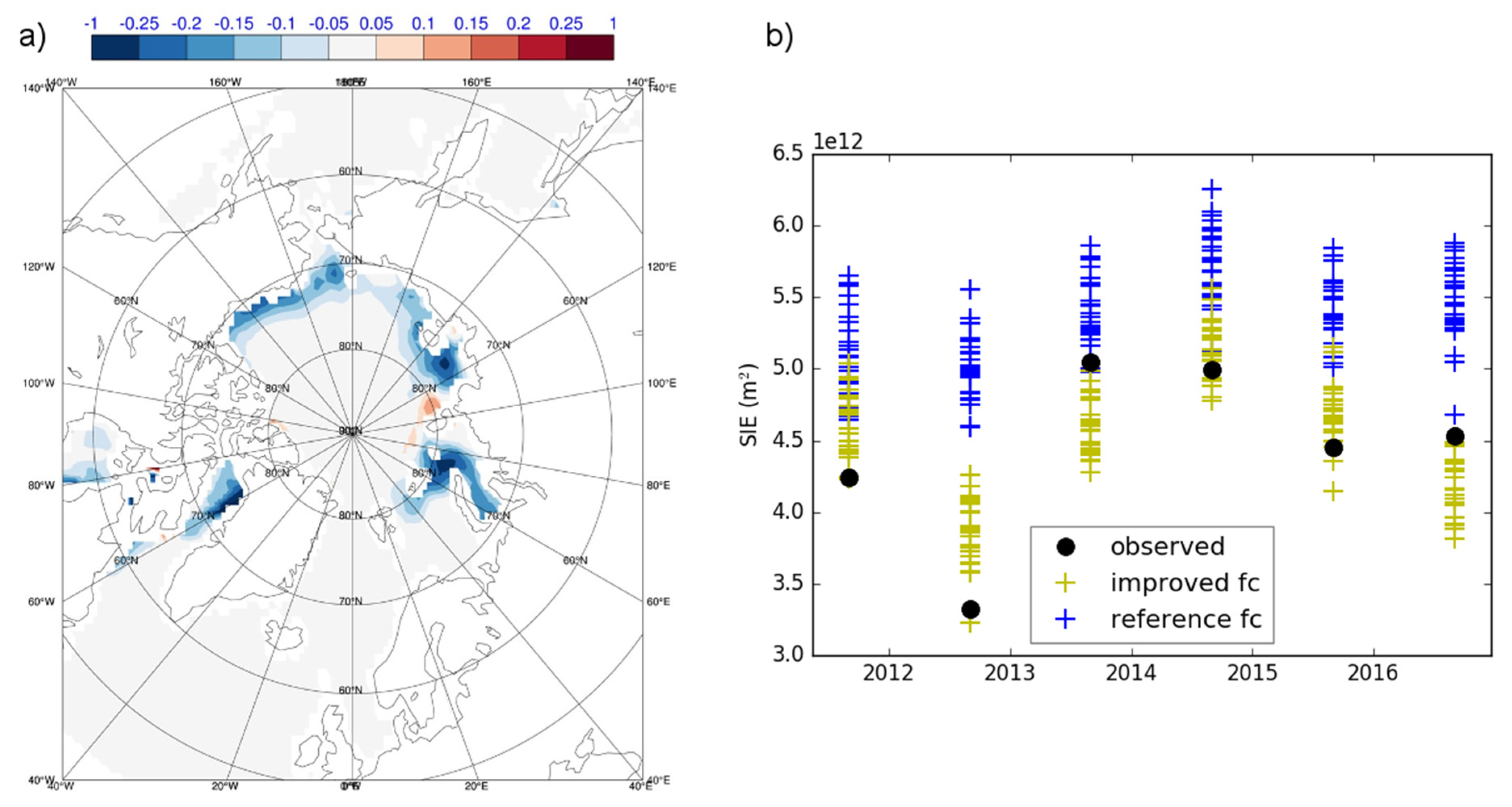
2.8. Improvements in Predicting Large-Scale Seasonal Sea-Ice Anomalies
3. Discussion
4. Conclusions
Author Contributions
Funding
Conflicts of Interest
Abbreviations
| AARI | Arctic and Antarctic Research Institute |
| AMSR2 | Advanced Microwave Scanning Radiometer 2 |
| ASCAT | Advanced Scatterometer in MetOp satellites of EUMETSAT |
| CS2SMOS | combined sea-ice thickness product from CryoSat-2 and SMOS data |
| C3S | Copernicus Climate Change Service |
| CIMR | Copernicus Imaging Microwave Radiometer |
| CMDD | cumulative melting degree day index |
| CMEMS | Copernicus Marine Environment Monitoring Service |
| CORDIS | Community Research and Development Information Service by European Commission |
| CRISTAL | Copernicus Polar Ice and Snow Topography Altimeter |
| DIR | degree of ice ridging |
| ECMWF | European Centre of Medium-Range Weather Forecast |
| EO | Earth Observation |
| ESA | European Space Agency |
| EUMETSAT | European Organisation for the Exploitation of Meteorological Satellites |
| FIS | Finnish Ice Service |
| FYI | first-year ice |
| HEM | helicopter-borne electromagnetic sensor for sea-ice thickness measurement |
| IMO | International Maritime Organization |
| JAXA | Japan Aerospace Exploration Agency |
| kNN | k-nearest neighbours classifier |
| MERIS | Medium Resolution Imaging Spectrometer |
| MPF | melt pond fraction |
| MPD2 | Melt Pond Detector 2 |
| MR | microwave radiometer |
| MSI | Melt Stage Index |
| MYI | multiyear ice |
| NASA | National Aeronautics and Space Administration |
| NCEP | U.S. National lefts for Environmental Prediction |
| NSCAT | NASA Scatterometer |
| NSIDC | U.S. National Snow and Ice Data left |
| NWP | numerical weather prediction |
| OIB | Operation Ice Bridge |
| OLCI | Ocean and Land Color Instrument |
| PC | polar class of a ship in IMO Polar Code |
| RIO | risk index outcome in IMO Polar Code |
| SAR | synthetic aperture radar |
| SIC | sea-ice concentration |
| SIRAL | SAR Interferometer Radar Altimete |
| SIT | sea-ice thickness |
| SMAP | Soil Moisture Active Passive satellite |
| SMOS | Soil Moisture and Ocean Salinity satellite |
| SPICES | Space-borne observations for detecting and forecasting sea-ice cover extremes, project by the EU’s Horizon 2020 programme |
| WMO | World Meteorological Organization |
| air temperature | |
| brightness temperature | |
| H-polarized brightness temperature | |
| V-polarized brightness temperature |
References
- JCOMM Expert Team on Sea Ice. Sea-Ice Nomenclature: Snapshot of the WMO Sea Ice Nomenclature WMO No. 259; World Meteorological Organization: Geneva, Switzerland, 2014; p. 121. [Google Scholar]
- Dirkson, A.; Denis, B.; Merryfield, W.J. A multimodel approach for improving seasonal probabilistic forecasts of regional Arctic sea ice. Geophys. Res. Lett. 2019, 46, 10844–10853. [Google Scholar] [CrossRef] [Green Version]
- Melsom, A.; Palerme, C.; Müller, M. Validation metrics for ice edge position forecasts. Ocean Sci. 2019, 15, 615–630. [Google Scholar] [CrossRef] [Green Version]
- Zampieri, L.; Goessling, H.F.; Jung, T. Bright prospects for Arctic sea ice prediction on subseasonal time scales. Geophys. Res. Lett. 2018, 45, 9731–9738. [Google Scholar] [CrossRef] [Green Version]
- Notz, D.; Jahn, A.; Holland, M.; Hunke, E.; Massonnet, F.; Stroeve, J.; Tremblay, B.; Vancoppenolle, M. The CMIP6 Sea-Ice Model Intercomparison Project (SIMIP): Understanding sea ice through climate-model simulations. Geosci. Model Dev. 2016, 9, 3427–3446. [Google Scholar] [CrossRef] [Green Version]
- Keeley, S.; Mogensen, K. Dynamic Sea Ice in the IFS; ECMWF Newsletter, 156; ECMWF: Reading, UK, 2018; pp. 23–29. [Google Scholar]
- Balan-Sarojini, B.; Tietsche, S.; Mayer, M.; Alonso-Balmaseda, M.; Zuo, H. Towards Improved Sea Ice Initialization and Forecasting with the IFS; ECMWF Technical Memoranda; ECMWF: Reading, UK, 2019. [Google Scholar]
- Balan-Sarojini, B.; Tietsche, S.; Mayer, M.; Balmaseda, M.A.; Zuo, H.; de Rosnay, P.; Stockdale, T.N.; Vitart, F. Year-round impact of winter sea ice thickness observations on seasonal forecasts. Cryosphere Discuss. 2020, in press. [Google Scholar]
- Space-Borne Observations for Detecting and Forecasting Sea Ice Cover Extremes | SPICES Project | H2020 | CORDIS | European Commission. Available online: https://cordis.europa.eu/project/id/640161 (accessed on 12 December 2019).
- Pedersen, L.T.; Tonboe, R.; Saldo, R.; Heygster, G.; Nicolaus, M.; Ozsoy-Cicek, B. Reference Datasets; H2020 SPICES Deliverable: D1.2, D1.3 & D1.4 ; Danish Meteorological Institute: Copenhagen, Denmark, 2016. [Google Scholar]
- Gegiuc, A.; Similä, M.; Karvonen, J.; Lensu, M.; Mäkynen, M.; Vainio, J. Estimation of degree of sea ice ridging based on dual-polarized C-band SAR data. Cryosphere 2018, 12, 343–364. [Google Scholar] [CrossRef] [Green Version]
- Aulicino, G.; Sansiviero, M.; Paul, S.; Cesarano, C.; Fusco, G.; Wadhams, P.; Budillon, G. A new approach for monitoring the Terra Nova Bay polynya through MODIS ice surface temperature imagery and its validation during 2010 and 2011 winter seasons. Remote Sens. 2018, 10, 366. [Google Scholar] [CrossRef] [Green Version]
- Wadhams, P.; Aulicino, G.; Parmiggiani, F.; Persson, P.O.G.; Holt, B. Pancake ice thickness mapping in the Beaufort Sea From wave dispersion observed in SAR imagery. J. Geophys. Res. Oceans 2018, 123, 2213–2237. [Google Scholar] [CrossRef]
- Wadhams, P.; Aulicino, G.; Parmiggiani, F.; Pignagnoli, L. Sea ice thickness mapping in the Beaufort Sea using wave dispersion in pancake ice—A case study with intensive ground truth. In Proceedings of the European Space Agency Living Planet Symposium, Prague, Czech Republic, 9–13 May 2016; Volume ESA SP-740. [Google Scholar]
- Aulicino, G.; Wadhams, P.; Parmiggiani, F. SAR pancake ice thickness retrieval in the terra nova bay (Antarctica) during the PIPERS Expedition in winter 2017. Remote Sens. 2019, 11, 2510. [Google Scholar] [CrossRef] [Green Version]
- Parmiggiani, F.; Moctezuma-Flores, M.; Wadhams, P.; Aulicino, G. Image processing for pancake ice detection and size distribution computation. Int. J. Remote Sens. 2019, 40, 3368–3383. [Google Scholar] [CrossRef]
- IMO. International Code for Ships Operating in Polar Waters (Polar Code); MEPC 68/21/Add.1, Annex 10; IMO: London, UK, 2015. [Google Scholar]
- IMO. Guidance on Methodologies for Assessing Pperational Capabilities and Limitations in Ice; MSC.1/Circ.15; IMO: London, UK, 2016. [Google Scholar]
- Rinne, E.; Similä, M. Utilisation of CryoSat-2 SAR altimeter in operational ice charting. Cryosphere 2016, 10, 121–131. [Google Scholar] [CrossRef] [Green Version]
- Rinne, E.; Sallila, H. Comparison of Sea Ice Type Estimates from Satellite Radar Altimetry and Auxiliary Sea Ice Type Products; H2020 SPICES Deliverable D3.3; Finnish Meteorological Institute: Helsinki, Finland, 2017. [Google Scholar]
- Iwamoto, K.; Ohshima, K.I.; Tamura, T. Improved mapping of sea ice production in the Arctic Ocean using AMSR-E thin ice thickness algorithm. J. Geophys. Res. Oceans 2014, 119, 3574–3594. [Google Scholar] [CrossRef]
- Nihashi, S.; Ohshima, K.I.; Tamura, T.; Fukamachi, Y.; Saitoh, S. Thickness and production of sea ice in the Okhotsk Sea coastal polynyas from AMSR-E. J. Geophys. Res. Oceans 2009, 114, C10025. [Google Scholar] [CrossRef] [Green Version]
- Shokr, M.; Asmus, K.; Agnew, T.A. Microwave emission observations from artificial thin sea ice: The ice-tank experiment. IEEE Trans. Geosci. Remote Sens. 2009, 47, 325–338. [Google Scholar] [CrossRef]
- Kaleschke, L.; Tian-Kunze, X.; Maaß, N.; Mäkynen, M.; Drusch, M. Sea ice thickness retrieval from SMOS brightness temperatures during the Arctic freeze-up period. Geophys. Res. Lett. 2012, 39, L05501. [Google Scholar] [CrossRef]
- Tian-Kunze, X.; Kaleschke, L.; Maaß, N.; Mäkynen, M.; Serra, N.; Drusch, M.; Krumpen, T. SMOS-derived thin sea ice thickness: Algorithm baseline, product specifications and initial verification. Cryosphere 2014, 8, 997–1018. [Google Scholar] [CrossRef] [Green Version]
- Huntemann, M.; Heygster, G.; Kaleschke, L.; Krumpen, T.; Mäkynen, M.; Drusch, M. Empirical sea ice thickness retrieval during the freeze-up period from SMOS high incident angle observations. Cryosphere 2014, 8, 439–451. [Google Scholar] [CrossRef] [Green Version]
- Schmitt, A.; Kaleschke, L. A consistent combination of brightness temperatures from SMOS and SMAP over Polar Oceans for sea ice applications. Remote Sens. 2018, 10, 553. [Google Scholar] [CrossRef] [Green Version]
- Zhao, T.; Shi, J.; Bindlish, R.; Jackson, T.J.; Kerr, Y.H.; Cosh, M.H.; Cui, Q.; Li, Y.; Xiong, C.; Che, T. Refinement of SMOS multiangular brightness temperature toward soil moisture retrieval and its analysis over reference targets. IEEE J. Sel. Top. Appl. Earth Observ. Remote Sens. 2015, 8, 589–603. [Google Scholar] [CrossRef] [Green Version]
- Schmitt, A.; Kaleschke, L. Combined SMOS and SMAP sea ice thickness Arctic (Version 1.0) [Data set]. Zenodo 2018. [Google Scholar] [CrossRef]
- Schmitt, A.; Kaleschke, L. Gridded Product of Sea Ice Thickness from SMOS and SMAP and Uncertainties; H2020 SPICES Deliverable D6.3; University of Hamburg: Hamburg, Germany, 2017. [Google Scholar]
- CERSAT—Monitoring Sea Ice with Scatterometers. Available online: http://cersat.ifremer.fr/oceanography-from-space/our-domains-of-research/sea-ice (accessed on 27 January 2020).
- Gohin, F.; Cavanié, A. A first try at identification of sea ice using the three beam scatterometer of ERS-1. Int. J. Remote Sens. 1994, 15, 1221–1228. [Google Scholar] [CrossRef]
- Girard-Ardhuin, F.; Ezraty, R. Enhanced Arctic sea ice drift estimation merging radiometer and scatterometer data. IEEE Trans. Geosci. Remote Sens. 2012, 50, 2639–2648. [Google Scholar] [CrossRef] [Green Version]
- Lavergne, T.; Eastwood, S.; Teffah, Z.; Schyberg, H.; Breivik, L.-A. Sea ice motion from low-resolution satellite sensors: An alternative method and its validation in the Arctic. J. Geophys. Res. 2010, 115, C10032. [Google Scholar] [CrossRef]
- Ricker, R.; Hendricks, S.; Kaleschke, L.; Tian-Kunze, X.; King, J.; Haas, C. A weekly Arctic sea-ice thickness data record from merged CryoSat-2 and SMOS satellite data. Cryosphere 2017, 11, 1607–1623. [Google Scholar] [CrossRef] [Green Version]
- Ricker, R.; Hendricks, S.; Girard-Ardhuin, F.; Kaleschke, L.; Lique, C.; Tian-Kunze, X.; Nicolaus, M.; Krumpen, T. Satellite-observed drop of Arctic sea ice growth in winter 2015–2016. Geophys. Res. Lett. 2017, 44, 3236–3245. [Google Scholar] [CrossRef] [Green Version]
- Ricker, R.; Girard-Ardhuin, F.; Krumpen, T.; Lique, C. Satellite-derived sea ice export and its impact on Arctic ice mass balance. Cryosphere 2018, 12, 3017–3032. [Google Scholar] [CrossRef] [Green Version]
- Ivanova, N.; Pedersen, L.T.; Tonboe, R.T.; Kern, S.; Heygster, G.; Lavergne, T.; Sørensen, A.; Saldo, R.; Dybkjær, G.; Brucker, L.; et al. Inter-comparison and evaluation of sea ice algorithms: Towards further identification of challenges and optimal approach using passive microwave observations. Cryosphere 2015, 9, 1797–1817. [Google Scholar] [CrossRef] [Green Version]
- Istomina, L.; Heygster, G.; Huntemann, M.; Schwarz, P.; Birnbaum, G.; Scharien, R.; Polashenski, C.; Perovich, D.; Zege, E.; Malinka, A.; et al. Melt pond fraction and spectral sea ice albedo retrieval from MERIS data—Part 1: Validation against in situ, aerial, and ship cruise data. Cryosphere 2015, 9, 1551–1566. [Google Scholar] [CrossRef] [Green Version]
- Heygster, G.; Istomina, L.; Zege, E.; Malinka, A.; Prikhach, A. Albedo and MPF Retrieval Methodology Using PM Observations; H2020 SPICES Deliverable D5.5; University of Bremen: Bremen, Germany, 2018. [Google Scholar]
- Polashenski, C.; Wright, N.; Perovich, D.K.; Song, A.; Deep, E.J. The impact of short-term heat storage on the ice-albedo feedback loop. In Proceedings of the American Geophysical Union, Fall Meeting, San Francisco, CA, USA, 12–16 December 2016; Volume C34A-02. [Google Scholar]
- Polashenski, C.; Golden, K.M.; Perovich, D.K.; Skyllingstad, E.; Arnsten, A.; Stwertka, C.; Wright, N. Percolation blockage: A process that enables melt pond formation on first year Arctic sea ice. J. Geophys. Res. Oceans 2017, 122, 413–440. [Google Scholar] [CrossRef]
- Eicken, H.; Krouse, H.R.; Kadko, D.; Perovich, D.K. Tracer studies of pathways and rates of meltwater transport through Arctic summer sea ice. J. Geophys. Res. 2002, 107, 8046. [Google Scholar] [CrossRef] [Green Version]
- Istomina, L.; Heygster, G.; Huntemann, M.; Marks, H.; Melsheimer, C.; Zege, E.; Malinka, A.; Prikhach, A.; Katsev, I. Melt pond fraction and spectral sea ice albedo retrieval from MERIS data—Part 2: Case studies and trends of sea ice albedo and melt ponds in the Arctic for years 2002–2011. Cryosphere 2015, 9, 1567–1578. [Google Scholar] [CrossRef] [Green Version]
- Comiso, J.C.; Cavalieri, D.J.; Markus, T. Sea ice concentration, ice temperature, and snow depth using AMSR-E data. IEEE Trans. Geosci. Remote Sens. 2003, 41, 243–252. [Google Scholar] [CrossRef]
- Brucker, L.; Markus, T. Arctic-scale assessment of satellite passive microwave-derived snow depth on sea ice using Operation IceBridge airborne data: Assessment of Snow Depth on Sea Ice. J. Geophys. Res. Oceans 2013, 118, 2892–2905. [Google Scholar] [CrossRef]
- Comiso, J.C.; Cavalieri, D.J.; Parkinson, C.L.; Gloersen, P. Passive microwave algorithms for sea ice concentration: A comparison of two techniques. Remote Sens. Environ. 1997, 60, 357–384. [Google Scholar] [CrossRef]
- Maaß, N.; Kaleschke, L.; Tian-Kunze, X.; Drusch, M. Snow thickness retrieval over thick Arctic sea ice using SMOS satellite data. Cryosphere 2013, 7, 1971–1989. [Google Scholar] [CrossRef] [Green Version]
- Rostosky, P.; Spreen, G.; Farrell, S.L.; Frost, T.; Heygster, G.; Melsheimer, C. Snow depth retrieval on Arctic sea ice from passive microwave radiometers—improvements and extensions to multiyear ice using lower frequencies. J. Geophys. Res. Oceans 2018, 123, 7120–7138. [Google Scholar] [CrossRef]
- Tonboe, R.; Winstrup, M.; Kreiner, M.; Lavergne, T.; Sørensen, A. Datasets of Ice and Snow Parameters for Ice Thickness Retrieval and for Input to WP8—Snow Depth on Sea Ice; H2020 SPICES Deliverable D4.3; Danish Meteorological Institute: Copenhagen, Denmark, 2018. [Google Scholar]
- Warren, S.G.; Rigor, I.G.; Untersteiner, N.; Radionov, V.F.; Bryazgin, N.N.; Aleksandrov, Y.I.; Colony, R. Snow depth on Arctic sea ice. J. Clim. 1999, 12, 1814–1829. [Google Scholar] [CrossRef]
- Johnson, S.J.; Stockdale, T.N.; Ferranti, L.; Balmaseda, M.A.; Molteni, F.; Magnusson, L.; Tietsche, S.; Decremer, D.; Weisheimer, A.; Balsamo, G.; et al. SEAS5: The new ECMWF seasonal forecast system. Geosci. Model Dev. 2019, 12, 1087–1117. [Google Scholar] [CrossRef] [Green Version]
- Zakhvatkina, N.; Smirnov, V.; Bychkova, I. Satellite SAR data-based sea ice classification: An overview. Geosciences 2019, 9, 152. [Google Scholar] [CrossRef] [Green Version]


© 2020 by the authors. Licensee MDPI, Basel, Switzerland. This article is an open access article distributed under the terms and conditions of the Creative Commons Attribution (CC BY) license (http://creativecommons.org/licenses/by/4.0/).
Share and Cite
Mäkynen, M.; Haapala, J.; Aulicino, G.; Balan-Sarojini, B.; Balmaseda, M.; Gegiuc, A.; Girard-Ardhuin, F.; Hendricks, S.; Heygster, G.; Istomina, L.; et al. Satellite Observations for Detecting and Forecasting Sea-Ice Conditions: A Summary of Advances Made in the SPICES Project by the EU’s Horizon 2020 Programme. Remote Sens. 2020, 12, 1214. https://0-doi-org.brum.beds.ac.uk/10.3390/rs12071214
Mäkynen M, Haapala J, Aulicino G, Balan-Sarojini B, Balmaseda M, Gegiuc A, Girard-Ardhuin F, Hendricks S, Heygster G, Istomina L, et al. Satellite Observations for Detecting and Forecasting Sea-Ice Conditions: A Summary of Advances Made in the SPICES Project by the EU’s Horizon 2020 Programme. Remote Sensing. 2020; 12(7):1214. https://0-doi-org.brum.beds.ac.uk/10.3390/rs12071214
Chicago/Turabian StyleMäkynen, Marko, Jari Haapala, Giuseppe Aulicino, Beena Balan-Sarojini, Magdalena Balmaseda, Alexandru Gegiuc, Fanny Girard-Ardhuin, Stefan Hendricks, Georg Heygster, Larysa Istomina, and et al. 2020. "Satellite Observations for Detecting and Forecasting Sea-Ice Conditions: A Summary of Advances Made in the SPICES Project by the EU’s Horizon 2020 Programme" Remote Sensing 12, no. 7: 1214. https://0-doi-org.brum.beds.ac.uk/10.3390/rs12071214