Drill-Core Mineral Abundance Estimation Using Hyperspectral and High-Resolution Mineralogical Data

Abstract

Due to the extensive drilling performed every year in exploration campaigns for the discovery and evaluation of ore deposits, drill-core mapping is becoming an essential step. While valuable mineralogical information is extracted during core logging by on-site geologists, the process is time consuming and dependent on the observer and individual background. Hyperspectral short-wave infrared (SWIR) data is used in the mining industry as a tool to complement traditional logging techniques and to provide a rapid and non-invasive analytical method for mineralogical characterization. Additionally, Scanning Electron Microscopy-based image analyses using a Mineral Liberation Analyser (SEM-MLA) provide exhaustive high-resolution mineralogical maps, but can only be performed on small areas of the drill-cores. We propose to use machine learning algorithms to combine the two data types and upscale the quantitative SEM-MLA mineralogical data to drill-core scale. This way, quasi-quantitative maps over entire drill-core samples are obtained. Our upscaling approach increases result transparency and reproducibility by employing physical-based data acquisition (hyperspectral imaging) combined with mathematical models (machine learning). The procedure is tested on 5 drill-core samples with varying training data using random forests, support vector machines and neural network regression models. The obtained mineral abundance maps are further used for the extraction of mineralogical parameters such as mineral association.

1. Introduction

Exploration campaigns are fundamental steps towards the discovery and evaluation of mineral deposits required to fulfil the global demand of raw materials. Drilling is an essential part of exploration surveys and consists of the extraction of long cylindrical core samples from underground areas associated with relevant exploration potential. Traditionally, drill-cores are visually analyzed by on-site geologists, who document characteristics such as mineralization type, lithology, structures and alteration types [1]. Subsequently, core samples are used for laboratory-based geochemical and mineralogical measurements to complement core logging results. While bulk geochemical analyses are often available for entire boreholes, quantitative mineralogical information is usually restricted to selected representative regions of interest. Standard quantitative analyses include X-Ray diffraction (XRD) applied on powder samples [2] or Scanning Electron Microscopy (SEM) based image analyses techniques [3] applied on polished thin sections prepared from areas of interest in the drill-cores. Additionally, qualitative mineralogical analyses are performed through optical microscopy on thin sections. These laboratory techniques provide valuable mineralogical information and derived mineralogical and metallurgical parameters, but they are of small scale, highly time-consuming, destructive, and rather expensive. This represents a challenge since thousands of meters of core are acquired during exploration campaigns.

Hyperspectral imaging is currently being used in the mining and exploration industries as an alternative tool to complement traditional logging techniques and to provide a rapid and non-invasive analytical method to obtain mineralogical information [4,5,6,7]. Typical hyperspectral core imaging systems can deliver data from a whole core tray (which holds approximately 5 m of core) in a matter of seconds. Available sensors cover a wide range of the electromagnetic spectrum and record data in several hundreds of contiguous spectral bands. Minerals have different spectral responses in specific portions of the electromagnetic spectrum. These responses are influenced by the vibrational and electronic absorption processes dependent on the bonds between atoms and electron orbitals [8]. Sensors covering the visible to near-infrared (VNIR) and short-wave infrared (SWIR) are commonly used to identify and estimate the relative abundance of minerals such as phyllosilicates, amphiboles, carbonates, iron oxides and hydroxides as well as sulphates [9].

Because of the increasing interest in hyperspectral data in the raw materials industry, with a wealth of hyperspectral data becoming available, the development of methods to effectively analyze these data is required. Traditional mapping methods include the use of spectral reference libraries (e.g., USGS spectral library) for mineral identification and mapping on hyperspectral imagery [10,11]. Slightly more automatic approaches, such as band ratios, or wavelength parameters such as position, depth and width of the absorption features are also used to map the distribution and relative abundance of specific minerals [12,13,14]. One of the most common procedures makes use of some of available tools in a software called Environment for Visualizing Images (ENVI, Exelis Visual Information Solutions, Boulder, Colorado). Such tools comprise endmember extraction, identification of the minerals using the Spectral Analysis or Material Identification by comparison to a specific library in the software (e.g., in ENVI) or online reference (e.g., USGS), and finally the mineral mapping task using similarity measure algorithms or determination of partial abundances using unmixing algorithms [5,15,16,17].

Although these approaches may produce good results, they require continuous expert input and thus, they tend to be time-consuming and difficult to automate for large dataset analysis. More importantly, the performance of available unmixing algorithms highly relies on the determination of the number of end-members and the selection of their representative spectra. In drill-core hyperspectral data, highly mixed pixels of hardly pure mineral associations represent a challenge. Methods such as unmixing, band ratios and minimum wavelength analysis can only provide mineral abundances for spectrally diagnostic phases. Additionally, due to the nature of the hyperspectral data and the spatial resolution allowed by commercially available sensors, the estimation of important mineralogical parameters in the characterization of complex ores (e.g., mineral association), is currently challenging.

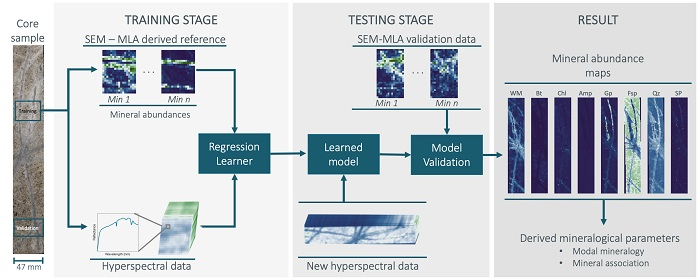
We propose a novel machine learning approach to estimate mineral quantities in drill-core hyperspectral data. The procedure comprises four steps: 1) drill-core hyperspectral scanning (VNIR –SWIR), 2) computing mineral abundances in a small but representative area of a drill-core by using high-resolution mineralogical analyses (e.g., SEM-based image analyses using a Mineral Liberation Analyser), 3) linking the mineral abundances in this small area to their corresponding spectra by a multivariate regression model, and 4) estimating mineral abundances for the whole drill-core hyperspectral data by using the learned model. The multivariate regression problem in the proposed scheme is solved using three algorithms: random forest (RF), support vector machines (SVM) and feedforward artificial neural networks (FF-ANN). The proposed procedure allows the abundance estimation of the main mineral groups using their spectral characteristics (SWIR active) and using those SWIR active minerals additionally as proxies for the SWIR non-active minerals or mineral groups such as quartz, feldspar and sulphide. The obtained mineral abundance mapping results can be used for the calculation of additional mineralogical parameters, relevant to exploration and mining projects. As an example, the concept of mineral association at hyperspectral pixel scale based on relative abundances is introduced in the current study.

2. Data Acquisition

2.1. Hyperspectral Data

The hyperspectral data used in this study were acquired from unpolished halves of diamond drilling core samples with a SisuROCK drill-core scanner equipped with an AisaFENIX hyperspectral sensor (Spectral Imaging Ltd., Oulu, Finland). The scanner is a fully automatic hyperspectral imaging workstation which employs a tray table which carries the drill-core trays or samples under the field-of-view of the spectrometer. The AisaFENIX camera implements two sensors to cover the VNIR and SWIR regions of the electromagnetic spectrum. The sensor specifications and acquisition settings are presented in

Table 1. AisaFENIX sensor specification and setup for hyperspectral data acquisition.

Wavelength Range	VNIR 380–970 nm SWIR 970–2500 nm	Integration Time	VNIR 15 ms SWIR 4 ms
Sampling Distance	VNIR 1.7 nm SWIR 5.7 nm	Spatial Binning	VNIR 2 SWIR 1
Number of Bands	450	Frame Rate	15 Hz
Samples	384	Scanning Speed	25.06 mm/s
Spatial Resolution	1.5 mm/pixel	Field of View (FOV)	32.3°
Detector	CMOS (VNIR) Stirling cooled MCT (SWIR)	Spectral Binning	VNIR 4 SWIR 1

.

The conversion from radiance to reflectance of the hyperspectral data was performed within the acquisition software (LUMO Scanner version 2018-5, Spectral Imaging Ltd., Oulu, Finland) using PTFE reference panels (>99% VNIR and >95% SWIR). To correct the sensor-specific optical distortions (i.e., fish-eye and slit-bending effects on the images) and the spatial shift between the VNIR and SWIR sensors, the toolbox MEPHySTo [18] was used. To avoid bands with little or no coherent information, the data were spectrally resampled to 480—2500 nm by removing the first 30 bands. The Savitzky–Golay filter was applied to decrease noise while preserving spectral features [19]. Principal component analysis (PCA) [20] was performed on the hyperspectral dataset for data dimensionality reduction and de-correlation while preserving 99.9% of the information.

2.2. Scanning Electron Microscopy-Based Mineral Liberation Analysis

Regions considered representative based on visual observations for the mineralogical variation within the drill-core samples were cut and prepared into polished thin sections. The preparation process consisted of grinding and polishing the sample surface followed by coating with a thin carbon layer to avoid surface charging during data acquisition. The grinding and polishing led to the removal of around 300 µm of material between the surface analyzed with the hyperspectral sensor and the surface subjected to the high-resolution mineralogical analysis. Considering the sample morphology and orientation of structural features the mineralogical variation is considered negligible for the encountered shift.

The quantitative mineralogical data were acquired from the thin sections using an automated approach. The analyses were carried out using Scanning Electron Microscope (SEM)-based Mineral Liberation Analysis (MLA) [3,21]. For this, a FEI Quanta 650 F field emission SEM instrument (FEI, Hillsboro, OR, USA), equipped with two Bruker Quantax X-Flash 5030 energy dispersive X-ray (EDX) detectors (Bruker, Billerica, MA, USA) and the MLA Suite software package (version 3.1.4.686, FEI, Hillsboro, OR, USA) were used. The grain-based X-ray mapping (GXMAP) mode was used to collect the mineralogical information as follows: the MLA software collects the back-scattered electron images (BSE) and uses them to effectively distinguish individual mineral grain boundaries based on the grey scale variations. The grey scale values of the BSE images are proportional to the average atomic density of the mineral grains and are used to provide a first mineralogical segmentation. The identification of minerals is performed based on X-ray analysis by placing a closely-spaced grid on a particle in the BSE image and collecting the X-ray data at the defined points of the grid. When dealing with fine grained material of lower size than the placed grid, the GXMAP mode allows us to collect additional spectra where variations in the BSE image are observed in between the measured grid points. Finally, the mineral is determined by matching the resultant spectrum of energy peaks with a reference library of X-ray spectra provided by the instrument company (FEI, Hillsboro, OR, USA), or from sample extracted spectra analyzed based on peak locations and intensities [22]. Specifications of the operating conditions used in this study are shown in

Table 2. Operating conditions and parameters used for the acquisition of high-resolution SEM-MLA mineralogical data.

SEM Settings		MLA Settings
Acceleration voltage (kV)	25	Pixel size (µm)	3
Probe current (nA)	10	Step size (pixels)	6 × 6
Frame width (pixels)	1500	Acquisition time (ms)	5
BSE calibration (Au)	254	Minimum grain size (pixels)	4

.

For classification, a mineral list was developed using the mineral reference editor in online mode. The resulting mineral list contained a total of 59 entries. However, for the integration of the HSI with SEM-MLA, further grouping was performed in this paper, such as considering all feldspars in one class, all white micas in another or, all sulphides, sulphosalts and gold in another. Accessory minerals were included in the final grouping labelled as “others”. As a result, ten main mineral groups are considered: white mica (WM), biotite (Bt), chlorite (Chl), amphibole (Amp), carbonate (Cb), gypsum (Gp), feldspar (Fsp), quartz (Qz), sulphide (Sp) and other.

3. Data Description

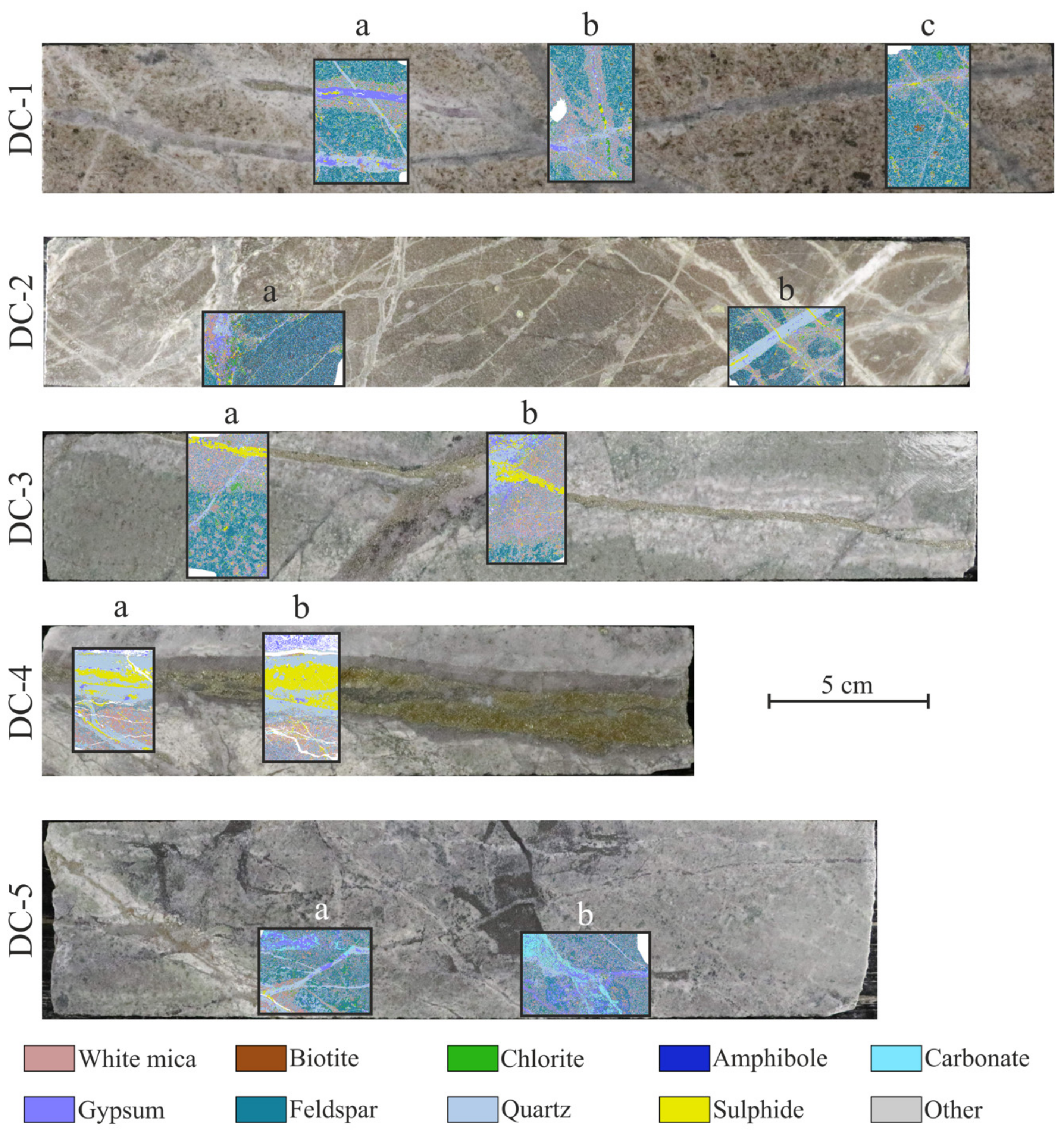
For testing the proposed methodology, 5 samples, labelled DC-1 to DC-5, from different locations within the Bolcana porphyry copper-gold system [23,24,25,26] were analyzed. Hyperspectral images were acquired on the halves cores after which thin sections were prepared from selected regions of interest and analyzed by SEM-MLA. Each region is further labelled as a, b and/or c starting from the left-hand side of the drill-core sample as illustrated in Figure 1. The ore minerals in the studied system are chalcopyrite, bornite, covellite, chalcocite and gold. Gold is dominantly present as fine inclusions in pyrite and chalcopyrite. The main encountered alteration types are potassic, sodic—calcic, phyllic and argillic. In the studied samples the first three are present, some samples presenting a transitional character and are described in this section. Please see Sillitoe, 2010 [27] for details on the mineralogical characteristics of the alteration styles typically associated with porphyry Cu-Au systems.

While the summary of the results for each sample is presented in the results section, an emphasis is made on DC-1 in order to illustrate all the potential information that can be extracted using the proposed methodology. Therefore, a more detailed description of this sample is available in the current section. Sample DC-1 consists of a diorite porphyry. Hydrothermal alteration in this sample appears transitional between potassic, represented by the presence of biotite and potassic feldspar and sodic-calcic characterized by the plagioclase-chlorite assemblage. Chlorite is more abundant than biotite in the first two thin sections, “a” and “b”. The third thin section, though, due to the lower vein density and implicit associated alteration presents significant amounts of biotite disseminated as well as in clusters in the matrix. Plagioclase feldspar is dominant in all three thin sections, near the veins however, an increase in potassic feldspar is observed.

Thin section “a” of sample DC-1 captures three main vein types: an oblique early quartz vein which exhibits a low intensity white mica alteration halo likely associated with a younger cross-cutting gypsum vein that has a sulphide centerline and a wide white mica-chlorite alteration halo (top). The alteration halo here is mica-dominant in the proximity of the vein and chlorite-dominant towards its edges. The third vein present in section “a” consists of quartz with a gypsum centerline and a spotty, low intensity white mica alteration halo (bottom). Thin section “b” captures three main vein types as well: two sub-vertical veins consist of variable ratios of gypsum and quartz and are surrounded by a strong white mica low-chlorite alteration halo. Compositionally, these veins appear to be a mixture between the first and third veins mentioned for thin section “a”; they have, however, a different morphology. In proximity to sub-horizontal veinlets in the lower half of the thin section, an increase in the pyrite and chlorite content is observed. The two sub-horizontal veinlets show strong similarity with the horizontal veins in the first thin section. The alteration intensity surrounding the sub-horizontal veinlets appears to be related to complex interactions with pre-existing veinlets in this area of section “b”. Thin section “c” hosts several fine veinlets, of highest width, the two cross-cutting ones near the top of the thin section. The veinlets consist of variable amounts of quartz, gypsum, pyrite and white mica and present a white mica and chlorite alteration halo. Similar to the subvertical veins in thin section “b” these veins appear to have a composition intermediate between the horizontal veins in thin section “a”. Unlike the two veins in thin section “b” however, the extent of the alteration halo is much lower.

Sample DC-2 is marked by pervasive potassic alteration characterized by the presence of K-feldspar, biotite and minor chlorite. Two main vein types are present in this sample: veins hosting dominantly sulphide which show a strong phyllic alteration halo caused by the late reaction of mineralizing hydrothermal fluids with the host rock. The second vein type comprises dominantly quartz with sulphide or with sulphide-calcium sulphate (gypsum or anhydrite) centerline. Additional veins of varying composition are present in the sample (left-hand side as illustrated in Figure 1). They appear to be the result of complex reopening and cross-cutting of the previously described veins. A sodic-phyllic rock matrix hosting two main vein-types characterizes sample DC-3. The first vein comprises of sulphide and presents a large white mica alteration halo. The second vein type consists predominantly of quartz, calcium sulphate and sulphide. The changing symmetry and mineral association in these latter veins indicate the reopening of an initially present quartz vein. Sample DC-4 is characterized by the presence of intense phyllic alteration in the matrix related to the thick pyrite-quartz-gypsum vein cross-cutting the sample. Additional fine veinlets comprising mostly quartz and pyrite are cutting the mica-rich matrix. The matrix in sample DC-5 consists of dominantly feldspar and subordinately white mica. Three main vein types can be observed in the samples: a sulphide dominant vein with a broad white mica alteration halo, quartz veinlets and carbonate iron-oxide veins which show low or absent alteration halos.

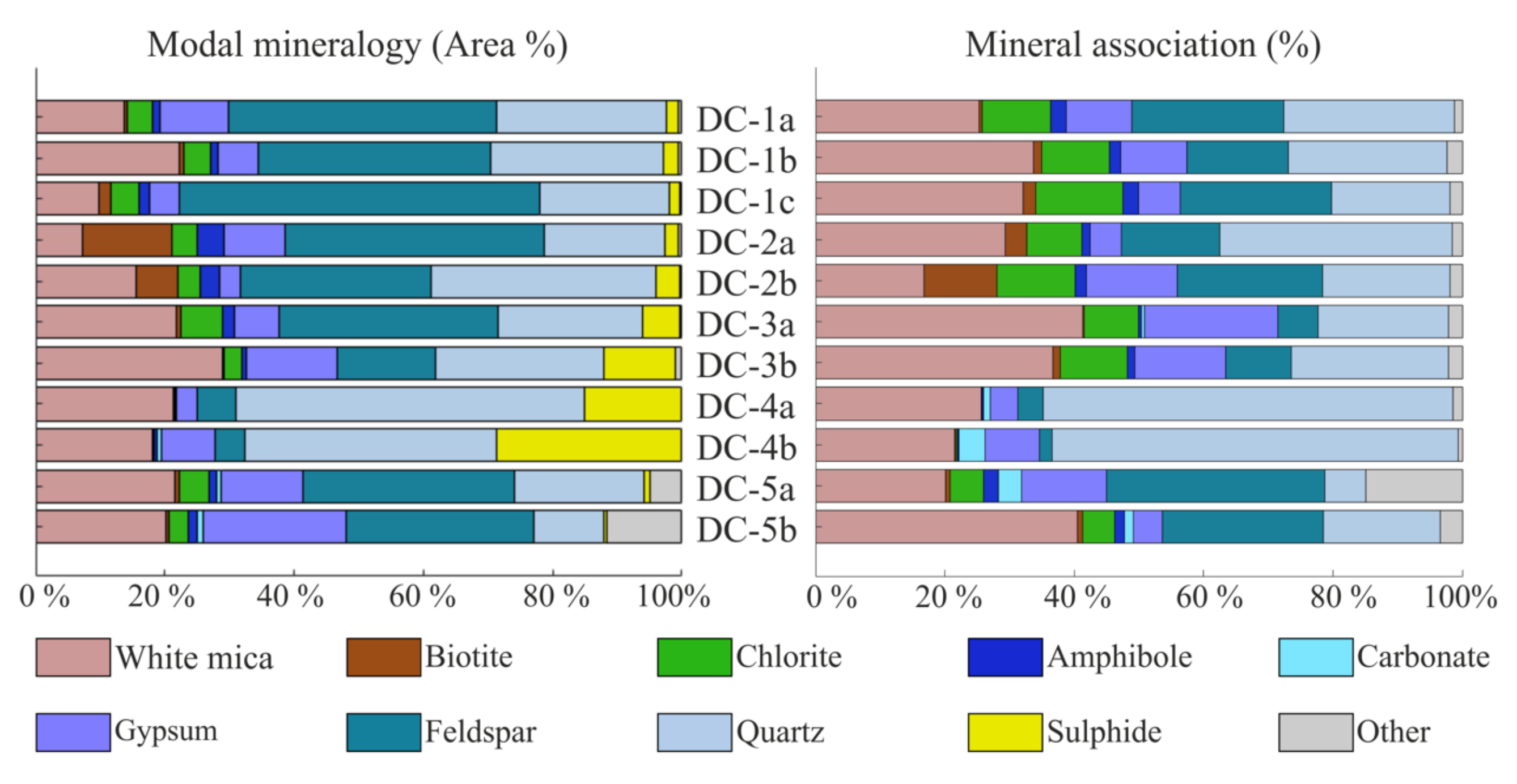
For the understanding of the modal composition of the available thin sections, the abundances of the minerals or mineral groups for all the analyzed thin sections are illustrated in the bar charts in Figure 2 (left). For most samples, quartz and feldspar represent the main rock-forming minerals. There is, however, a variation in the extent of alteration of feldspar to white mica ranging from low (DC-2a) to high (DC-4). In most of the analyzed samples, the amphibole is to a large extent altered to chlorite and/or biotite. Biotite is only present in significant amounts in sample DC-2 and DC-1 “c”. The variation of the quartz, carbonate and gypsum contents is related to the surface abundance of the veins and veinlets filled mostly by these three minerals. While quartz and gypsum are present in significant amounts in all thin sections, carbonate is mainly represented in sample DC-5. The class “sulphide” comprises mainly pyrite, chalcopyrite, bornite, chalcocite and covellite but minor amounts of native gold hosted as inclusions in pyrite and chalcopyrite is also considered. While pyrite is not an ore mineral by itself, it frequently represents the host of micron-size native gold inclusions. The sulphide content in the thin sections ranges from around 1 area % in DC-5b to almost 30 area % in DC-4b. The main target being the quantification and understanding of the distribution of sulphide minerals within the presented samples, their mineral association is also analyzed and presented in the bar chart in Figure 2 (right).

While an influence of the modal mineralogy can be observed on the mineral association, a strong increase in the white mica, chlorite, biotite, carbonate and gypsum can be seen. This is the result of the distribution of these minerals within or surrounding the veins also hosting the bulk of sulphides. The listed gangue minerals, unlike the sulphide, show distinct absorption features in the VNIR-SWIR region of the electromagnetic spectrum and may, therefore, be used as proxies for the distribution of the ore minerals.

4. Methodological Framework

4.1. HSI—SEM-MLA Data Integration

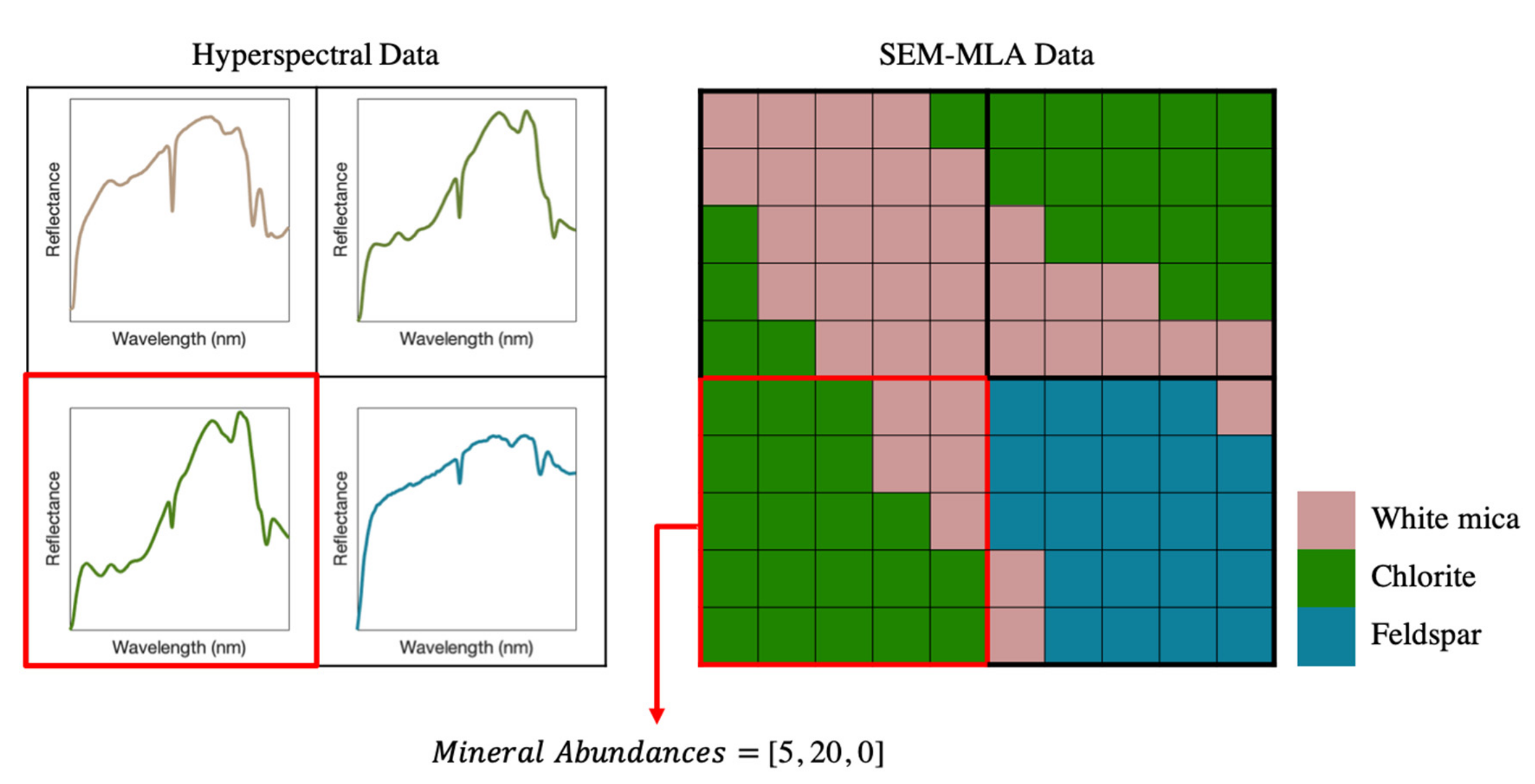
For the proposed approach, the SEM-MLA data is upscaled by adopting a re-sampling procedure. The two-dimensional SEM-MLA mineral map with high spatial resolution is transformed to a three-dimensional mineral abundance map with the lower spatial resolution of the hyperspectral data [7]. The third dimension consists of the relative abundance of each mineral present in each SEM-MLA map re-sampled to the hyperspectral pixel size (Figure 3). Note that a co-registration stage is needed after the re-sampling of the SEM-MLA data. Following Acosta et al., 2019, the structural features, such as veins, the mineral composition, and spectral responses are used to find suitable tie points. As a result of the co-registration each pixel where the SEM-MLA data is available is characterised by two vectors: the hyperspectral feature vector Xi of dimension d (i.e., the number of bands in the hyperspectral data) or r (number of extracted features) and a mineral abundance vector Yi containing the corresponding fractional abundances of the minerals identified by SEM-MLA.

Once the hyperspectral and SEM-MLA data are co-registered, they are divided into training and testing. For this procedure the following approach is adopted:

• Using 50% randomly selected pixels from all thin section regions within one drill-core sample for training, the remaining drill-core hyperspectral data for testing. The validation is performed using the remaining 50% data points from the MLA regions.
• Using 1 thin section for training and the second for testing and validation for all drill-core samples.
• For DC-1, where 3 thin sections are available, an additional test is performed using 2 thin sections for training and the last for testing and validation.

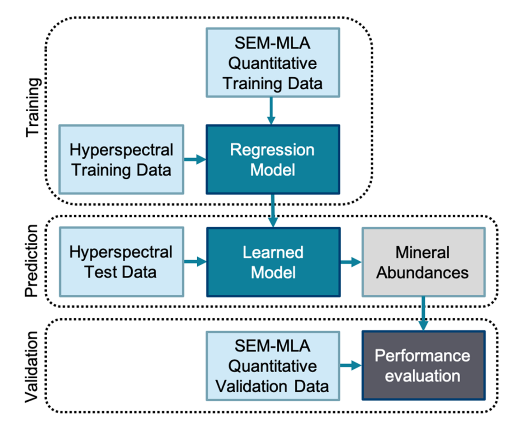
As can be seen from the main flowchart, shown in Figure 4, the proposed workflow is carried out in three main phases. In the training phase, different regression models (i.e., RF, SVM and FF-ANN) are trained following any of the three approaches mentioned before. In the prediction phase, the learned models are used to predict the mineral abundances on the entire drill-core samples. Finally, in the validation phase, the root mean square error (RMSE) [28] is calculated on the remaining SEM-MLA test data to assess the performance of the abundance mapping.

Two analysis types are further performed on the resulting mineral abundance data. For each validation set, the modal mineralogy is calculated based on the average abundance of each mineral phase in each pixel and compared to the modal mineralogy data obtained from SEM-MLA. Additionally, the concept of mineral association is adapted from the automated mineralogy field (Figure 2). There, the mineral association is calculated by counting the neighboring pixels to a specific target mineral. Slight changes in the approach have to be made when the spatial resolution of the hyperspectral data is used. The association of the main target group, i.e., sulphide, is a fundamental aspect in the present geological study. For each hyperspectral pixel the estimated mineral abundance of each mineral phase, except of the target, is normalized by the abundance of sulphide in the respective pixel. While this approach does not directly indicate the grain contact between the two minerals (or rather mineral groups) it can be seen as the probability of their association and occurrence at the scale of hyperspectral data resolution. The mineral association is calculated on the ground truth or validation data as well as on the estimated abundances calculated with the three proposed regression models.

4.2. Random Forest Regression

Random forests (RFs) are currently one of the most popular supervised learning techniques for classification and regression problems [29,30,31]. RFs are ensemble-based algorithms in which several models (trees) are running in parallel with randomized sampling. The individual results of these trees are then combined into the final prediction by an averaging process [32]. For regression purposes, the trees are given numerical values as predictors whereas in classification problems they are fed class labels. The RF technique is desirable in cases where only few training samples are available, as is usually the case in drill-core hyperspectral imaging.

4.3. Support Vector Regression

The aim of support vector machines (SVMs) is to search for hyperplane decision boundaries to define a linear prediction model [33,34]. To locate and orientate the hyperplane, only the samples that are close to the hyperplane, so-called support vectors, have an influence. Therefore, SVMs perform well when a limited number of well-chosen training samples are available [31,33,34]. This model can be used for classification or regression tasks. SVMs were originally proposed to solve linear problems. However, decision boundaries are often non-linear. To cope with the non-linearity problem, the kernel-based SVMs were introduced to project the data points into a higher dimensional feature space where the samples are linearly separable [31].

4.4. Artificial Neural Network Regression

Artificial neural networks have become some of the most popular methods in regression and classification because of their success in capturing the non-linearity relation between independent and dependent variables [35]. We chose a so-called “feedforward neural network” (FF-ANN) [36], as it fits the requirements of the problem at hand. In a feedforward network, each neuron in one layer is directly connected to neurons of the next layer with no cycle between layers. The applied neural network consists of an input layer, one hidden layer, and an output layer. Each neuron of a layer is computed by the product sum of the neurons of the previous layers plus a bias for the neuron [31]. A sigmoid function is applied for activation.

5. Experimental Results

In order to showcase the suitability of the proposed approach, the first drill-core sample presented in the data section (DC-1) is used. The remaining four samples have been analyzed following the same procedure. A summary of the results is presented in this section followed by a complete illustration of the results in Appendix A. Additionally, all numerical results are presented in the Electronic Supplementary Materials (Table S1).

From the entire drill-core sample (DC-1), the VNIR-SWIR hyperspectral data of size 33 by 189 pixels. The 420 spectral bands cover wavelengths from 480 nm to 2500 nm. The hyperspectral data is subjected to PCA leading to the reduction in dimensionality to 13 principal components in the third dimension. Moreover, the high-resolution mineralogical data obtained from representative regions (thin sections “a”, “b” and “c”) were used. In the thin section regions of the drill-core sample, each hyperspectral pixel covers an area of 1.5 by 1.5 mm², which is characterized by about 250,000 pixels in the SEM-MLA image. The fractional abundances were computed by considering the frequency of the identified minerals in the corresponding region of the SEM-MLA image for each hyperspectral pixel. To have more consistent results, we considered a threshold of 250,000 pixels (i.e., a hyperspectral pixel size) in each thin section region, for discarding minerals which have a very low frequency in the original SEM-MLA image. Taking this factor into consideration, the following six mineral classes remained: white mica (WM), biotite (Bt), chlorite (Chl), amphibole (Amp), gypsum (Gp), feldspar (Fsp), quartz (Qz), sulphide including sulphosalts and native gold (SP); less abundant minerals were grouped as “other”. Because of the low abundance of biotite and accessory minerals in thin sections “a” and “b”, the number of mineral classes considered was decreased accordingly. The test setups presented in the methodological framework section are used.

Cross-validation has been used to find the optimal parameters in order to train three models by internally resampling the training data. The main tested parameter ranges for each algorithm are presented in

Table 3. Parameters and parameter ranges for the choice in optimum setup of the three tested algorithms.

RF	SVM	FF-ANN
Nb. of trees – 500 : 600	Kernel – Radial Basis Function	Training function – Scaled conjugate gradient backpropagation
	Cost – 2 : 0.5 : 4	Nb. of hidden layers – 1
	Sigma – 5 : 0.5 : 7	Nb. of neurons – 30 : 10 : 80

. The setups were chosen according to the lowest associated root-mean-square error (RMSE) based on cross-validation within 30 averaged iterations.

5.1. Mineral Abundance and Association Mapping

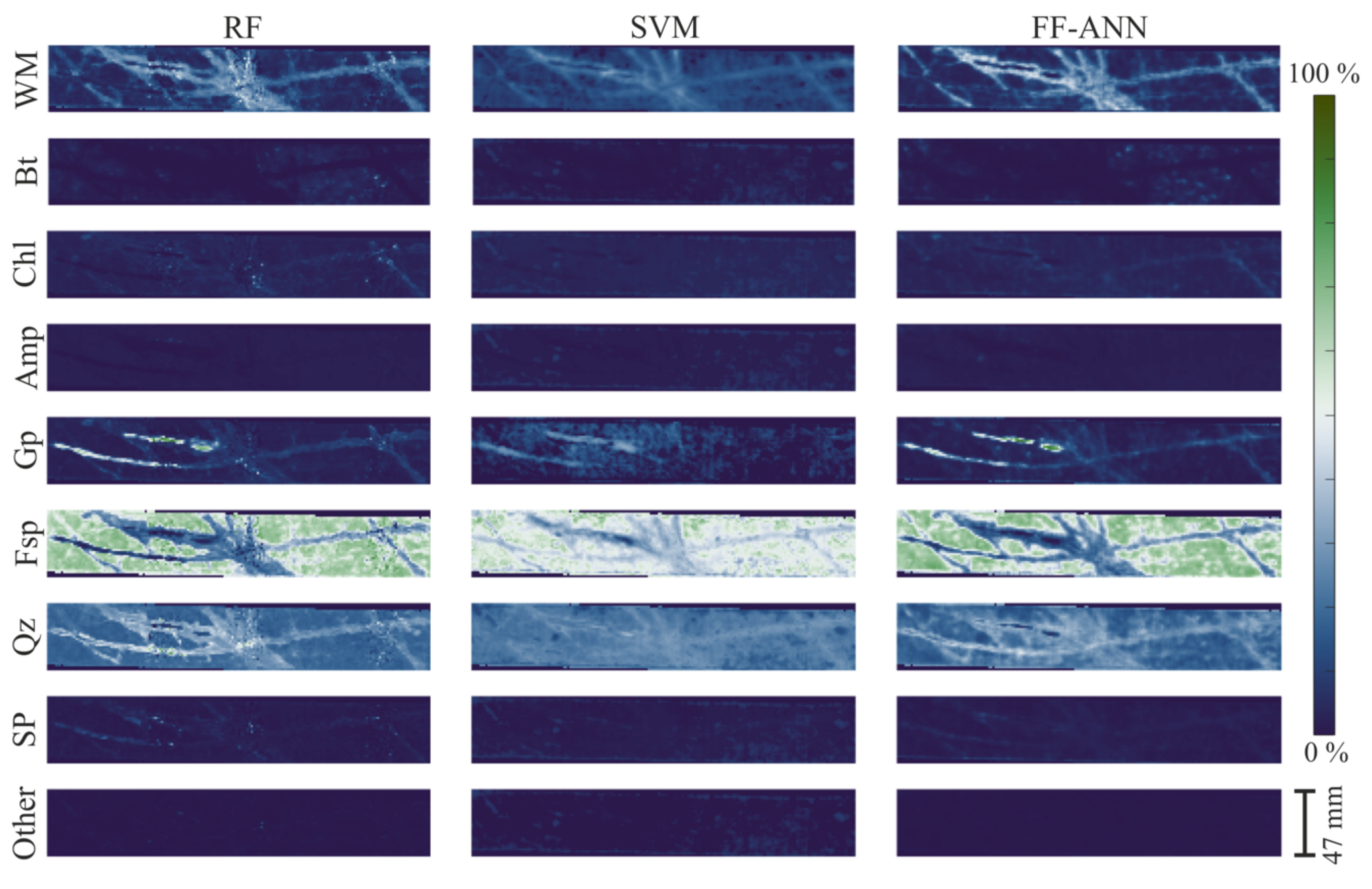
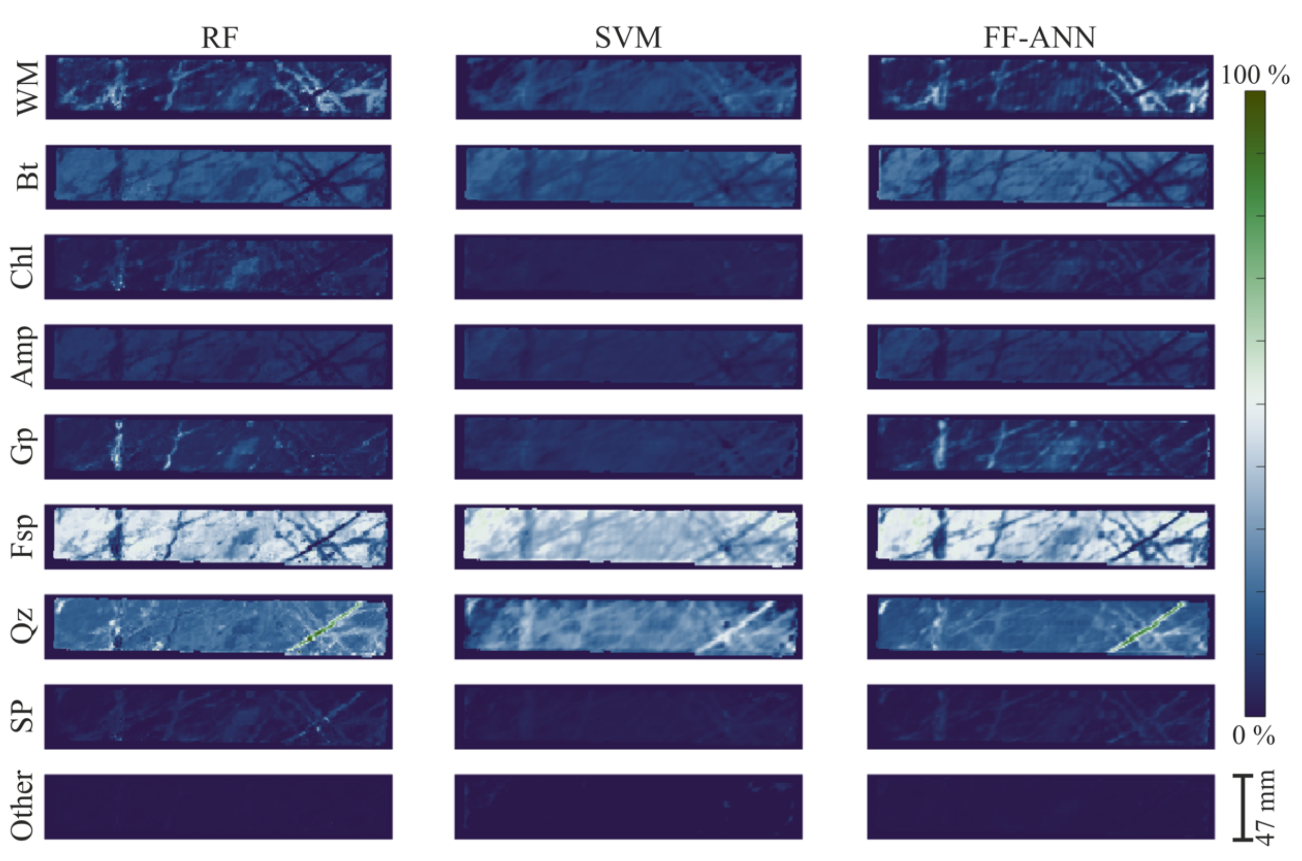
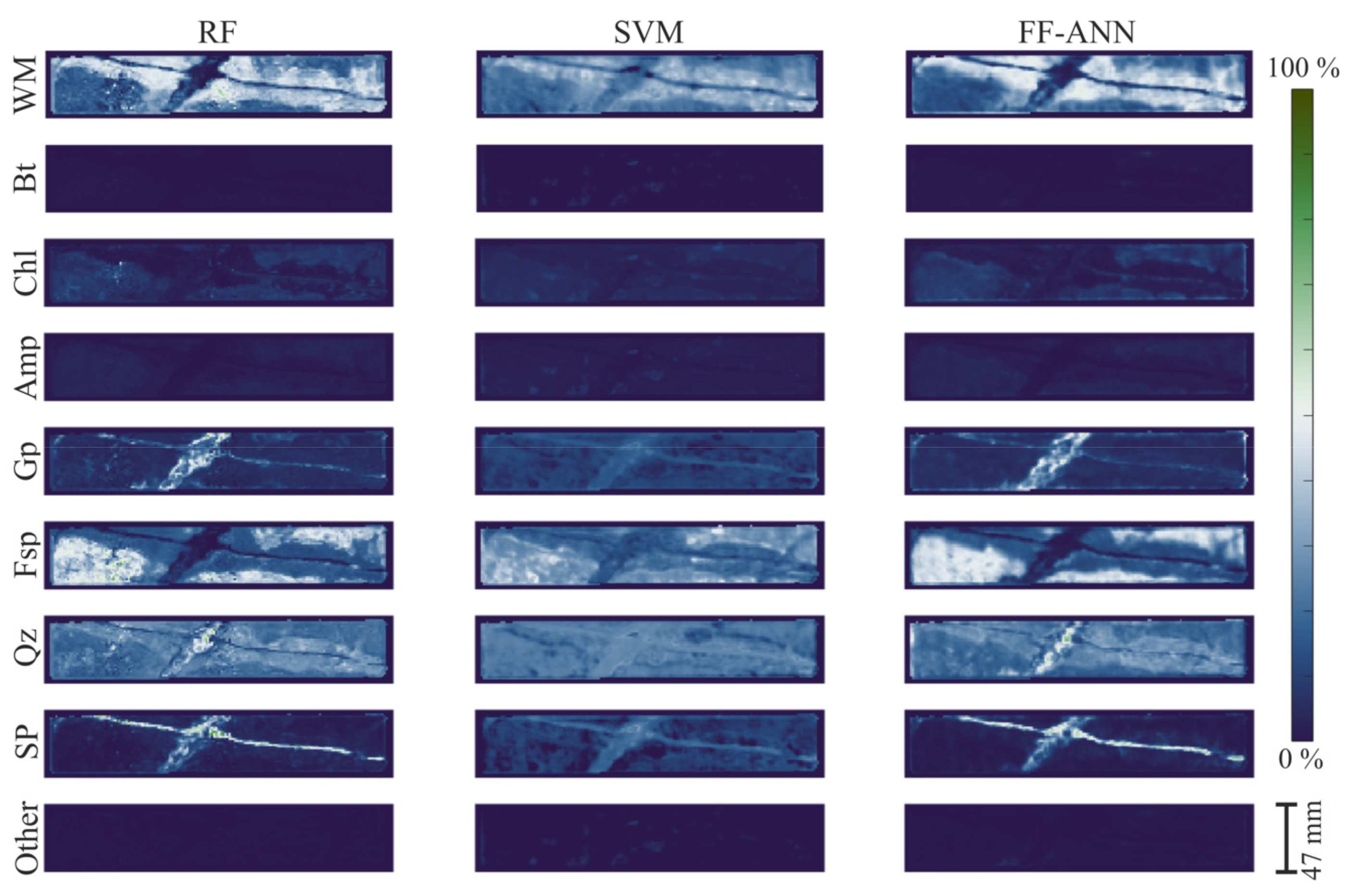
With the first experimental setup, presented in the methodological framework, 50% randomly distributed samples of the available thin section regions were used to train the regression models the mineral abundances estimation in the entire drill-core sample (Figure 5). Based on the visual analysis of the core and results analysis, RF and FF-ANN show better results in estimating the abundance of minerals with local distribution and small concentrations. With respect to matrix mineralogy, while biotite is well estimated by SVM in comparison with RF and FF-ANN, other major components of the matrix such as feldspar present a rather poor estimation. Similar performances of the algorithms can be observed for vein mineral components such as gypsum and sulphide.

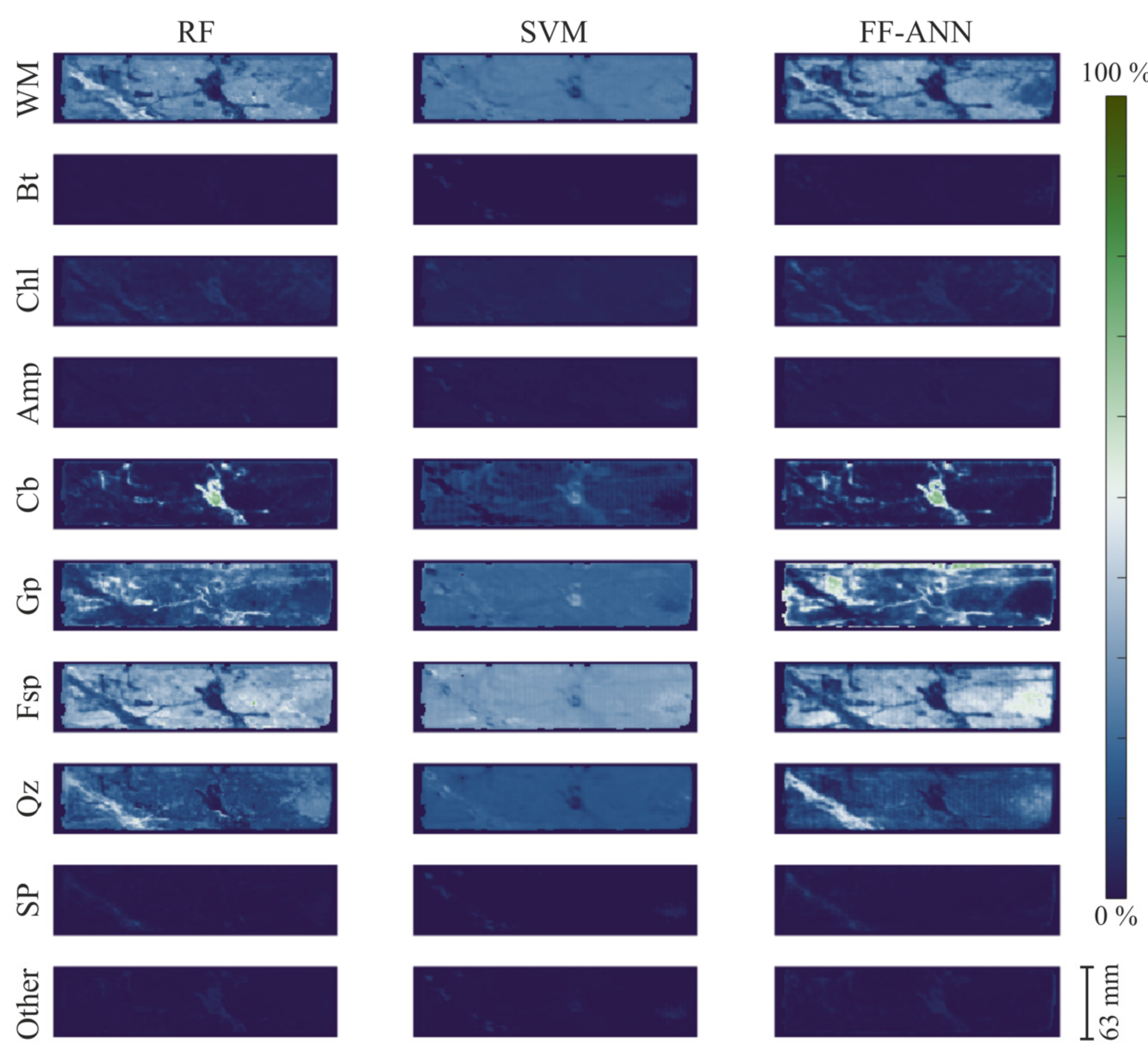
With regards to the samples DC-2 (Figure A1), DC-3 (Figure A3), DC-4 (Figure A5) and DC-5 (Figure A7), using 50% of the available ground truth data for training, RF and FF-ANN show good, similar performances, while SVM shows limitations specifically in transitional areas between veins and matrix. Among the SWIR-diagnostic minerals, white mica, biotite and carbonate appear well mapped in all the samples, chlorite is slightly underestimated in samples DC-2 and DC-3 and gypsum is overestimated in sample DC-5. Among the SWIR non-diagnostic minerals, quartz shows the highest mapping inconsistencies between vein and matrix, particularly for samples DC-4 and DC-5. Sulphide, however, appears to be well mapped in most areas of the samples.

The quantitative evaluation of the mineral abundance mapping through the calculation of the RMSE supports the visual observations (

Table 4. Evaluation of the three tested methods for the mineral abundance mapping of DC-1 through overall RMSE and per class RMSE values.

Method	RMSE	RMSE per Class
		WM	Bt	Chl	Amp	Gp	Fsp	Qz	SP	Other
RF	0.07	0.06	0.06	0.06	0.06	0.06	0.05	0.08	0.06	0.05
SVM	0.10	0.12	0.03	0.05	0.01	0.12	0.21	0.12	0.04	0.02
NN	0.08	0.06	0.06	0.07	0.06	0.06	0.07	0.09	0.07	0.07

). All three tested algorithms present low RMSEs and prove suitable to be used for mineral abundance mapping purposes. RF shows the lowest overall RMSE of 0.07, followed by FF-ANN with 0.08 and SVM with 0.1. Regarding the per class RMSE, RF and FF-ANN show similar results with the largest error associated with quartz, which can be the result of the lack of diagnostic absorption features in the VNIR-SWIR regions of the electromagnetic spectrum. SVM on the other hand shows larger per class errors for feldspar together with an increase in the error on white mica distribution. This can be explained by a misclassification between the two mineral groups. The mineral association of the sulphide in each pixel was calculated from the results of the mineral abundance mapping. Based on this calculation an equivalent overall performance of the methods was obtained (

Table 5. Evaluation of the three tested methods for the mineral association mapping of DC-1 through overall RMSE and per class RMSE values.

Method	RMSE	RMSE per Class
		WM	Bt	Chl	Amp	Gp	Fsp	Qz	Other
RF	0.05	0.05	0.00	0.01	0.00	0.02	0.13	0.05	0.00
SVM	0.06	0.06	0.01	0.02	0.00	0.02	0.15	0.06	0.00
NN	0.05	0.05	0.00	0.01	0.00	0.02	0.13	0.05	0.00

). For each of the methods, the error for the association of sulphide with feldspar is the largest.

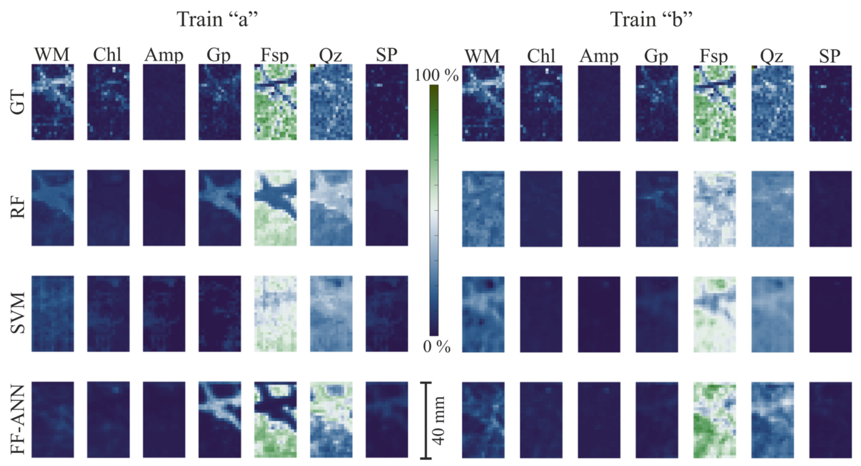
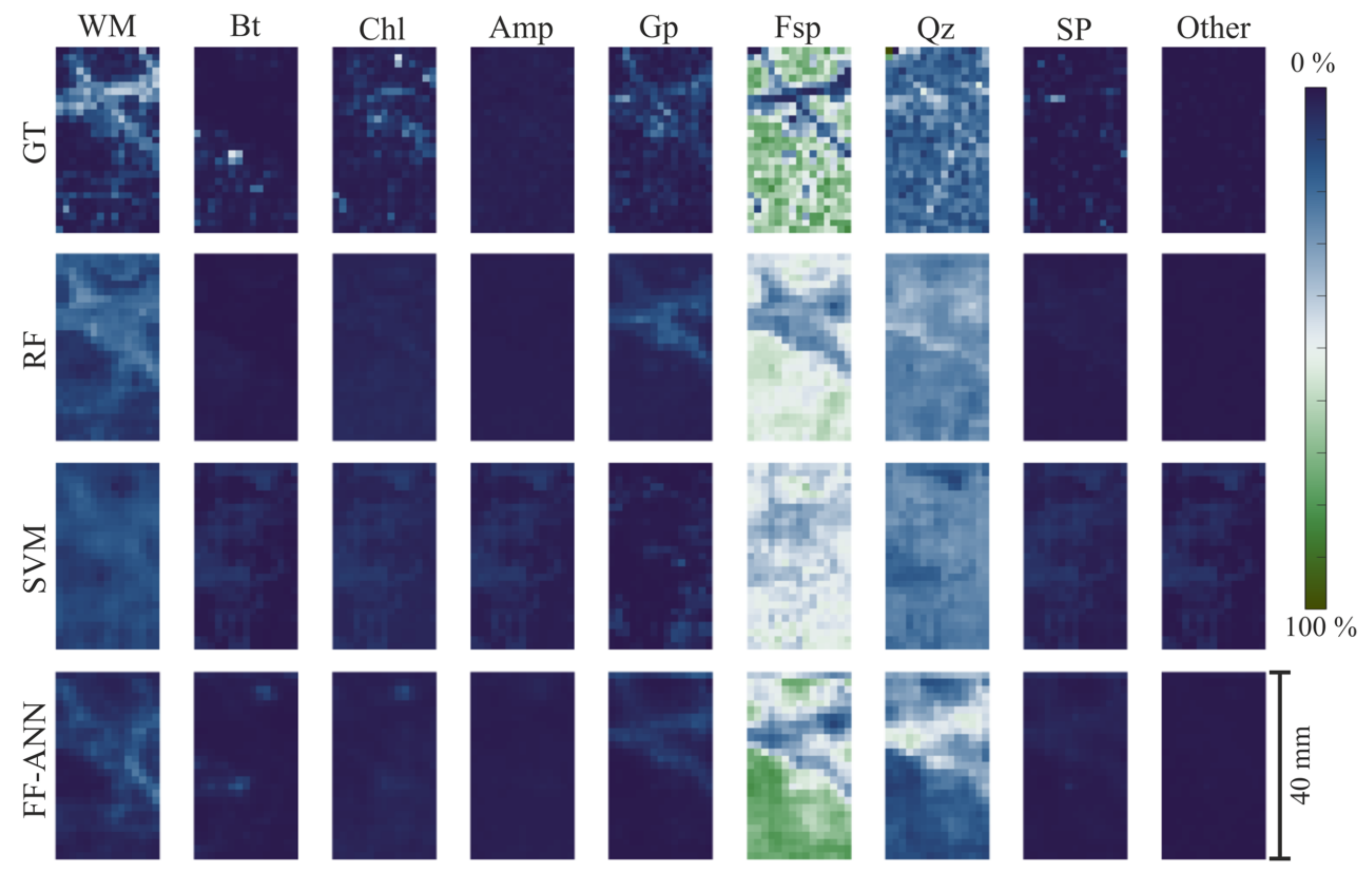
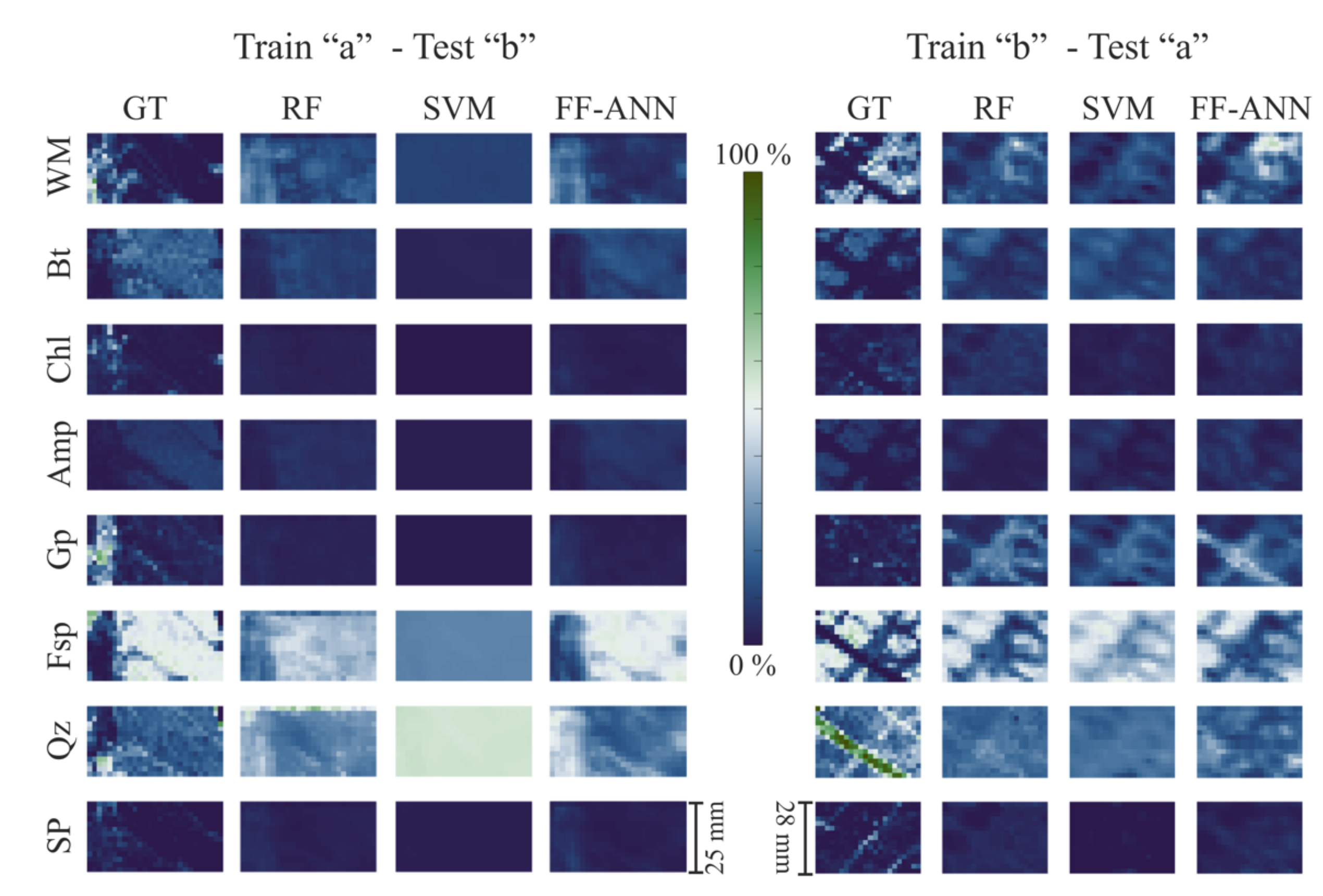
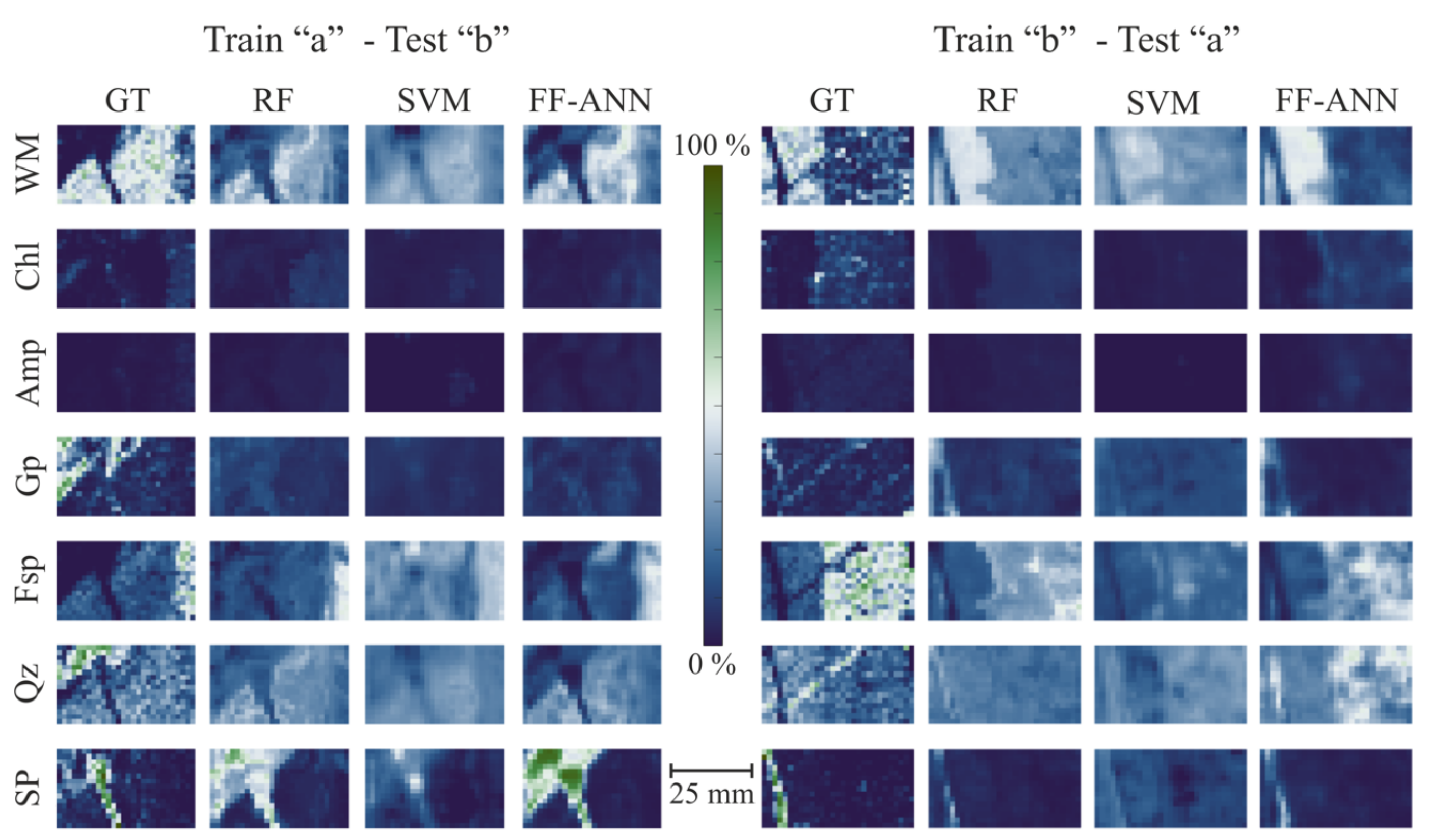
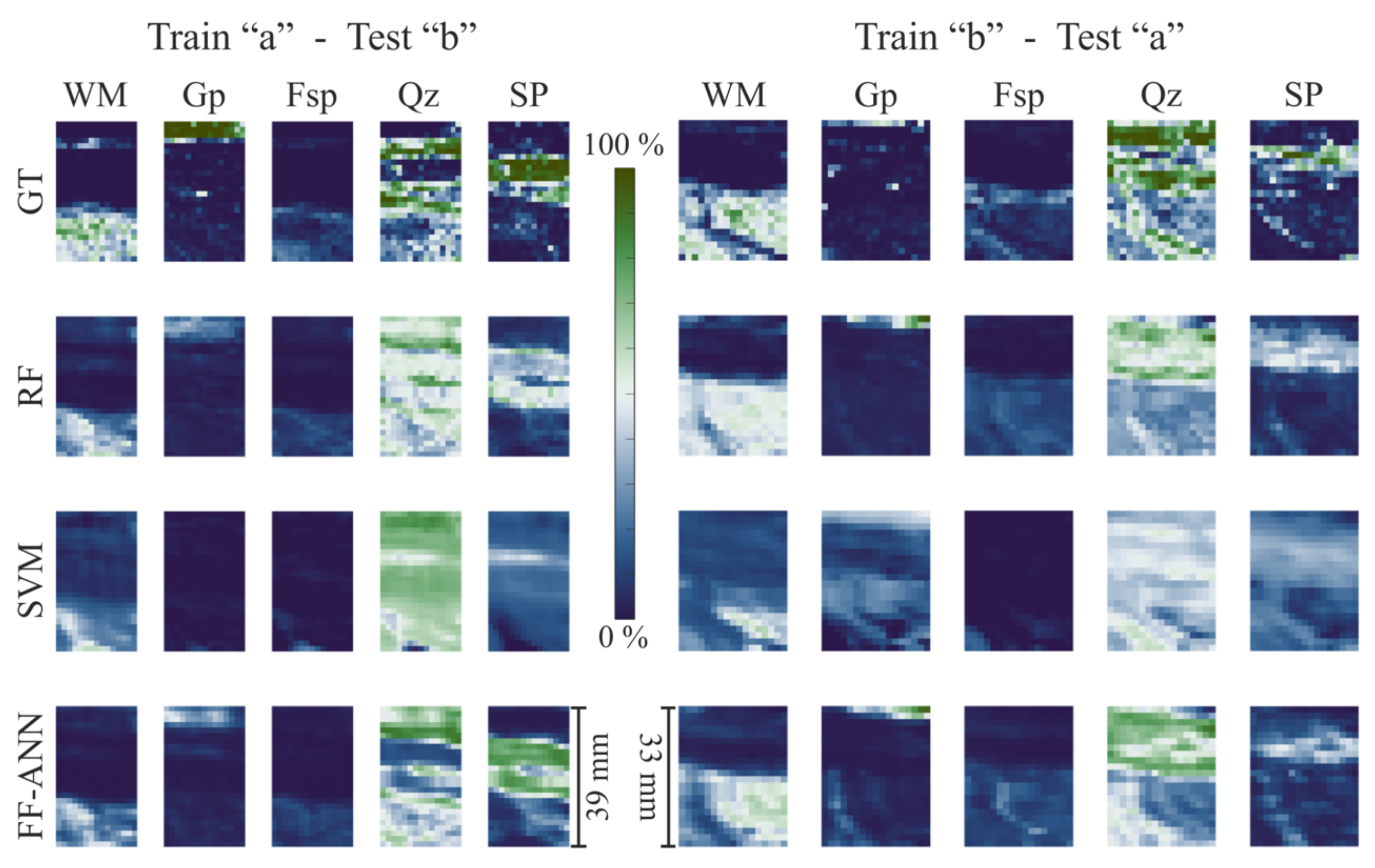
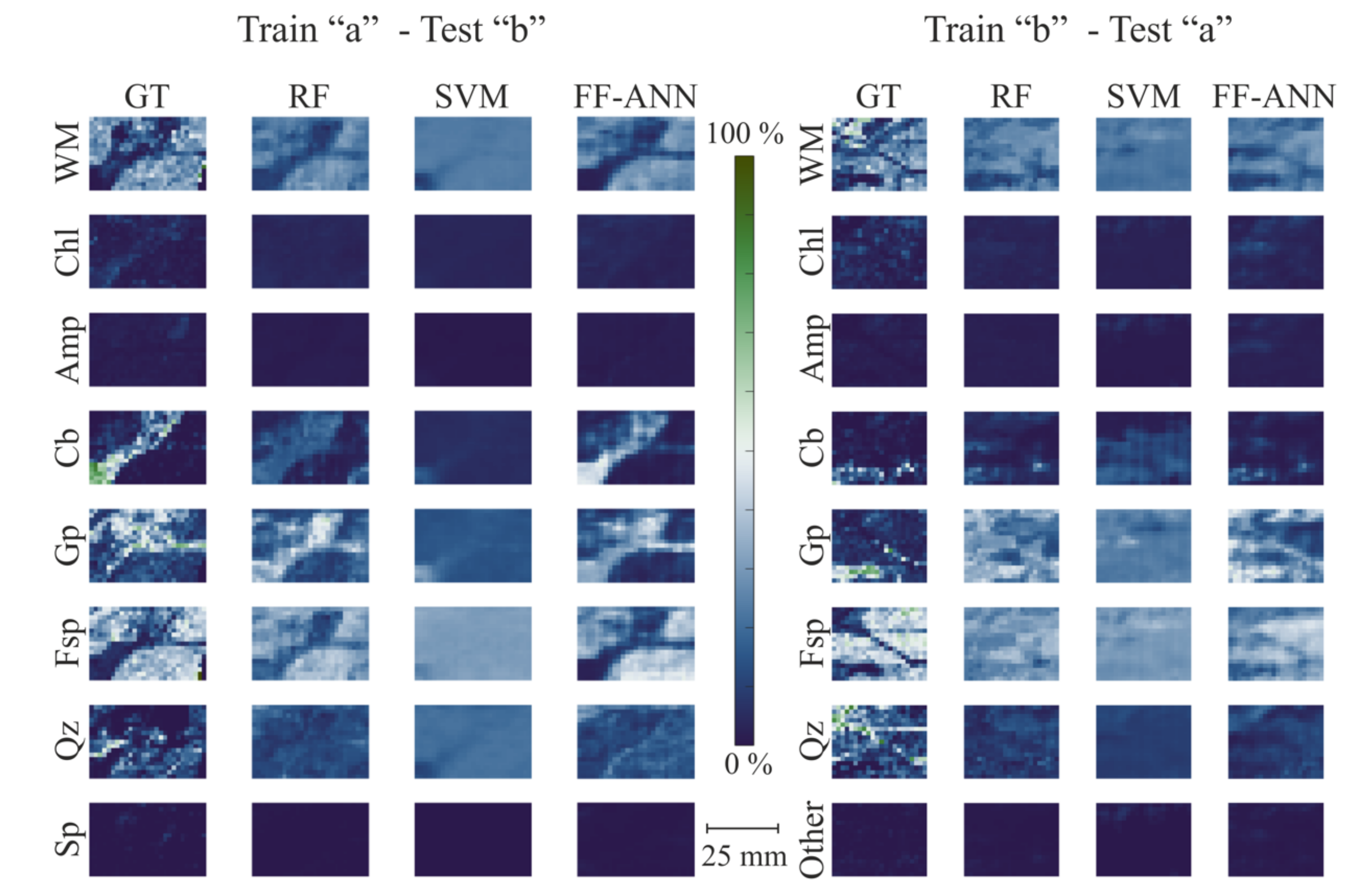
To assess the importance of sampling and representativeness of the SEM-MLA regions, thin sections “a”, “b” (Figure 6) and “a + b” (Figure 7) of sample DC-1 were used for training the models in order to estimate the mineral abundance and association in thin section “c”.

For the three used methods, strong differences in the estimates of sample “c” mineralogy can be observed when using thin sections “a” and “b” for training (

Table 6. Evaluation of the three tested methods for the mineral abundance mapping of DC-1 thin section “c” through overall RMSE and per class RMSE values using different samples for training.

	Train and Valid. Data	Overall RMSE	RMSE per Class
			WM	Bt	Chl	Amp	Gp	Fsp	Qz	SP	Other
RF	50%–50% rand. sel	0.07	0.06	0.06	0.06	0.06	0.06	0.05	0.08	0.06	0.05
	Train a—Test—c	0.10	0.08		0.06	0.01	0.06	0.18	0.13	0.03
	Train b—Test—c	0.12	0.15		0.05	0.01	0.05	0.24	0.09	0.03
	Train a + b—Test c	0.08	0.09	0.04	0.05	0.01	0.04	0.18	0.11	0.03	0.01
SVM	50%–50% rand. sel	0.10	0.12	0.03	0.05	0.01	0.12	0.21	0.12	0.04	0.02
	Train a—Test—c	0.10	0.10		0.06	0.02	0.06	0.20	0.12	0.04
	Train b—Test—c	0.09	0.11		0.06	0.02	0.04	0.18	0.10	0.04
	Train a + b—Test c	0.09	0.09	0.05	0.06	0.03	0.07	0.21	0.09	0.05	0.03
FF-ANN	50”–50% rand. sel	0.08	0.06	0.06	0.07	0.06	0.06	0.07	0.09	0.07	0.07
	Train a—Test—c	0.17	0.12		0.07	0.02	0.14	0.28	0.27	0.06
	Train b—Test—c	0.12	0.12		0.07	0.02	0.06	0.25	0.14	0.04
	Train a + b—Test c	0.10	0.10	0.05	0.06	0.01	0.05	0.20	0.16	0.04	0.01

). The use of thin section “a” provides particularly better results for white mica and feldspar, which are confused using region “b” that hosts distinctly lower amounts of feldspar. On the other hand, using thin section “a” for training leads to an overestimation of the gypsum content. The use of both thin sections (“a” + “b”) for training improves the classification leading to lower overall and per class RMSE values. As for the remaining drill-core samples, RF outperforms SVM and FF-ANN for most training scenarios, except when using thin section “b” for training. A similar effect of sampling on the RMSE evaluation can be seen for the mineral association mapping of DC-1 in all the scenarios (

Table 7. Evaluation of the three tested methods for the mineral association mapping of DC-1 thin section “c” through overall RMSE and per class RMSE values using different samples for training.

	Train and Validation Data	Overall RMSE	RMSE per Class
			WM	Bt	Chl	Amp	Gp	Fsp	Qz	Other
RF	50%–50% rand. sel	0.05	0.05	0.00	0.01	0.00	0.02	0.13	0.05	0.00
	Train a—Test—c	0.06	0.05		0.04	0.01	0.05	0.05	0.10
	Train b—Test—c	0.03	0.04		0.03	0.00	0.01	0.01	0.02
	Train a + b—Test c	0.02	0.01	0.01	0.04	0.01	0.00	0.01	0.06	0.00
SVM	50%–50% rand. sel	0.06	0.06	0.01	0.02	0.00	0.02	0.15	0.06	0.00
	Train a—Test—c	0.05	0.05		0.02	0.02	0.07	0.06	0.06
	Train b—Test—c	0.04	0.05		0.05	0.01	0.01	0.02	0.05
	Train a + b—Test c	0.03	0.05	0.03	0.01	0.03	0.06	0.03	0.00	0.03
FF-ANN	50%–50% rand. sel	0.05	0.05	0.00	0.01	0.00	0.02	0.13	0.05	0.00
	Train a—Test—c	0.17	0.13		0.05	0.01	0.15	0.24	0.28
	Train b—Test—c	0.07	0.07		0.04	0.00	0.04	0.15	0.00
	Train a + b—Test c	0.05	0.09	0.00	0.05	0.01	0.02	0.06	0.10	0.00

).

For the remaining samples, each having two regions analyzed by SEM-MLA, the mineral abundance estimations obtained using the second setup are illustrated in Figure A2 (DC-2), Figure A4 (DC-3), Figure A6 (DC-4) and Figure A8 (DC-5).

The tested methods show similar results for mineral abundance and association mapping on the remaining four drill-cores (

Table 8. Methods evaluation for the mineral abundance and association mapping of the remaining four samples through overall RMSE and per class RMSE values using different data for training.

Sample ID	Train and Validation Data	Mineral Abundance Mapping			Mineral Association Mapping
		RF	SVM	FF-ANN	RF	SVM	FF-ANN
DC-2	50%–50% rand. sel	0.07	0.09	0.08	0.07	0.07	0.07
	Train a—Test—b	0.11	0.18	0.10	0.09	0.17	0.09
	Train b—Test—a	0.14	0.14	0.19	0.13	0.16	0.13
DC-3	50%–50% rand. sel	0.08	0.11	0.09	0.12	0.12	0.12
	Train a—Test—b	0.14	0.14	0.17	0.09	0.18	0.07
	Train b—Test—a	0.11	0.14	0.14	0.10	0.11	0.09
DC-4	50%–50% rand. sel	0.12	0.20	0.14	0.12	0.12	0.12
	Train a—Test—b	0.24	0.29	0.24	0.08	0.10	0.05
	Train b—Test—a	0.16	0.20	0.19	0.04	0.16	0.07
DC-5	50%–50% rand. sel	0.07	0.10	0.08	0.03	0.03	0.03
	Train a—Test—b	0.11	0.13	0.11	0.05	0.18	0.05
	Train b—Test—a	0.13	0.13	0.15

). Overall, RF performs best, followed by FF-ANN and then SVM. For samples DC-1, DC-2, DC-3 and DC-5 each method results in comparable errors where similar amounts of training data are used. For sample DC-4 the overall RMSE values are higher, exceeding 0.2 depending on training data. For each sample the selection of the training data location plays an important role that is reflected into the RMSE evaluation.

5.2. Modal Mineralogy

The modal mineralogy in area % is calculated by averaging the mineral abundances over the entire tested sample. To evaluate the modal mineralogy estimates sample DC-1 is used and the estimates are compared to the ground truth, using 50% of the available SEM-MLA data for training and 50% for testing (

Table 9. Ground truth and estimated modal mineralogy of the SEM-MLA test regions of DC-1, using 50% randomly selected data for training.

Method	Modal Mineralogy (Area %)
	WM	Bt	Chl	Amp	Gp	Fsp	Qz	SP	Other
GT	16.0%	1.1%	4.3%	1.8%	7.3%	42.3%	24.9%	1.8%	0.5%
RF	15.8%	1.1%	4.3%	1.7%	7.4%	42.2%	25.1%	2.0%	0.5%
SVM	14.2%	1.2%	3.8%	1.8%	7.8%	44.3%	24.4%	1.8%	0.6%
NN	15.8%	1.1%	4.3%	1.7%	7.3%	42.6%	24.8%	1.9%	0.5%

).

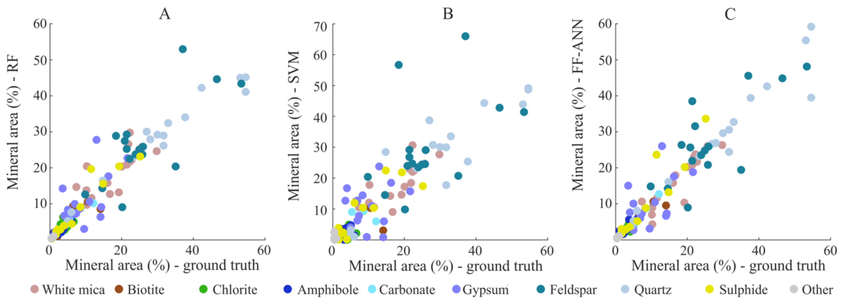
The estimates for all methods show good results with the highest RMSE value of 0.01 obtained with SVM. The complete modal mineralogy results are available in Table S1. The results for all the setups and all samples and methods are illustrated in Figure 8 by plotting the estimated values from RF (left), SVM (centre) and FF-ANN (right) against the ground truth values known from the re-sampled SEM-MLA data. The estimated and true values for RF and FF-ANN show overall a good correlation with local outliers related to mineral groups such as feldspar, as these do not have distinct spectral features in the VNIR-SWIR regions of the electromagnetic spectrum. Outliers can also be observed for white mica where the training and testing classes were unbalanced and confusions between mica and feldspar occurred. SVM, on the other hand, shows higher deviations from a linear correlation. Additionally, an important factor influencing the results is the data used for sampling. All test scenarios results are included in Figure 8 and as observed in the mineral abundance mapping results (Table 8), sampling plays a critical role in method performance.

5.3. Mineral Association

The overall mineral association is calculated by averaging the sulphide association in each classified pixel. The results for the setup consisting of 50% of the SEM-MLA regions of DC-1 for training and 50% for testing are presented in

Table 10. Ground truth and estimated mineral association of the SEM-MLA test regions of DC-1, using 50% randomly selected data for training.

Method	Sulphide Association
	WM	Bt	Chl	Amp	Gp	Fsp	Qz	Other
GT	21.0%	0.7%	5.6%	1.5%	9.9%	30.1%	30.5%	0.6%
RF	16.2%	1.1%	4.4%	1.8%	7.6%	42.8%	25.7%	0.5%
SVM	14.5%	1.2%	3.9%	1.9%	7.8%	45.1%	24.8%	0.6%
NN	16.2%	1.1%	4.4%	1.8%	7.5%	43.2%	25.3%	0.5%

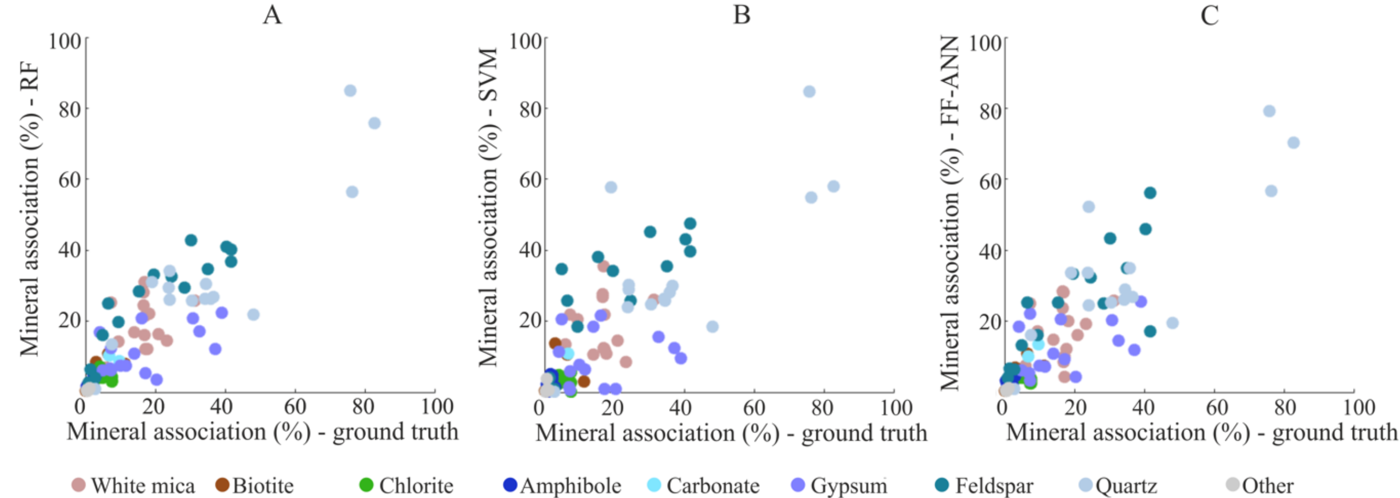
. For each regression method, the association of sulphide with white mica, chlorite, gypsum and quartz is underestimated, while the feldspar association is overestimated. The same tendency is observed for the rest of the calculated mineral associations in all samples and setups (Appendix A, Figure A1, Figure A2, Figure A3, Figure A4, Figure A5, Figure A6, Figure A7 and Figure A8). The relationship between ground truth and estimated data is illustrated in the scatter-plots in Figure 9. The results of the mineral association are strongly influenced by the estimation of the sulphide abundance as well as of the other mineral groups. Therefore, the highest errors in sulphide abundance mapping are consistent with the largest errors for sulphide association.

6. Discussion

The proposed approach for data preparation and analysis illustrates the potential to arrive at robust quantitative mineral abundance estimates from hyperspectral drill-core data—even for those minerals that do not have diagnostic absorption features in the VNIR-SWIR regions of the electromagnetic spectrum (e.g., feldspars, quartz, sulphides). Three regression methods were tested in this paper for mineral abundance estimation: random forest (RF), support vector machines (SVM) and feedforward artificial neural networks (FF-ANN). These methods were applied to quantify mineral abundances—also of minerals devoid of characteristic HS spectral features (here sulphide minerals). In addition, attempts were made to extract mineral association data from HS information at a lateral resolution far below the actual size of mineral grains in the studied ore. For this purpose, the abundance of each gangue mineral in each HS pixel is normalized to the content of ore minerals that are the main target in the currently studied porphyry system, thus constituting a rather simple proxy for the opportunity of two minerals or mineral groups to occur in direct contact with each other.

The abundance estimation of SWIR diagnostic mineral phases and groups is good overall, particularly for white mica, amphibole and chlorite. For the case of gypsum, however, due to its pervasive association with white mica in some training samples, errors in the abundance estimation occurred. Even though it is present in minor amounts in comparison to white mica, the estimation error can reach similar amplitudes as those of white mica. An additional reason for high errors associated with gypsum is related to its composition. The higher the degree of hydration of anhydrite towards gypsum the stronger and more distinct its absorption features. While SEM-MLA methods cannot measure the amount of water in the structure of the hydrated calcium sulphate, hyperspectral sensors are highly sensitive to these changes. Therefore, having training samples hosting mostly calcium sulphate with low amount of water can cause miss-estimation in test samples which may have low amounts of highly hydrated calcium sulphate. The local high errors in the estimation of biotite content can be assigned to the low amount of training samples containing relevant amounts of biotite. Sulphide is the main target in the current case study and this group comprises dominantly of pyrite, chalcopyrite, bornite, covellite, chalcocite, minor sulphosalts and native gold as an inclusion in the sulphides. While locally sulphide can be present as disseminations in the matrix, the highest fraction is present in veins. For all methods, the abundance estimation for SWIR non-diagnostic minerals is highly dependent on their association with the hydrothermal alteration minerals. To be able to estimate their abundance, representative sampling is required to avoid the erroneous estimation of these minerals based on local association with SWIR minerals that are not consistent at drill-core scale. For the analyzed samples the highest per-class errors are obtained for feldspar and quartz, both SWIR non-diagnostic minerals. In many cases feldspar was overestimated, particularly in samples where white mica abundance was underestimated. As white mica is present as an alteration product of feldspar in the proximity of veins, it can be assumed that the training samples consisted of lower alteration degrees of the feldspar to white mica while the test samples showed contrasting composition. As a result, feldspar particularly represented a bottleneck for the evaluation of the mineral association where their association with sulphide was in each case overestimated. Besides the fact that this mineral group does not show distinctive absorption features in the VNIR-SWIR regions of the electromagnetic spectrum, the spatial resolution of the used sensor can highly influence the misclassification and the overestimation in its association with sulphide. Feldspar is usually present in the host-rock matrix and is expected to have a low association with sulphide, usually being altered to white mica in the proximity of the sulphide-bearing veins. When the vein alteration halo is thinner than the spatial resolution of the sensor (here 1.5 mm), an increase in the apparent association of sulphide with feldspar is observed.

A potential limitation resides in the removal of the mineral fractions present in low concentrations (lower total surface abundance than the size of a hyperspectral pixel). Additionally, the compositional variation of minerals such as white mica and chlorites is not analyzed in the current work, but could be performed by auxiliary methods such and minimum wavelength analysis.

To evaluate the performance of the three regression methods employed in this paper, the RMSE was calculated. In general, for the mineral abundance estimation RF performed well and derived the lowest errors. The errors produced by FF-ANN tend to be higher than by SVMs in all the test scenarios, except in the case when 50% of the ground truth was randomly selected as the training data. This highlights the capabilities of SVM to perform well when a limited number of training samples are available and of FF-ANN to achieve good results when enough training data are available. The random selection of the training data allows for a more representative sampling per class than it is for the other two test scenarios where one thin section is used for training and the other thin section is used for the test. This is because certain minerals can be more abundant in one part of the core than in the other as it was previously stated for DC-1 in the results section. Although larger per class RMSE are obtained by minerals without diagnostic absorption features in the VNIR-SWIR, this is countered by random sampling and errors decrease considerably. From the analysis and evaluation of the results obtained by the utilized regression methods, the RF algorithm is the most suitable for the current dataset.

The proposed framework allows for fast evaluation of the modal mineralogy of analyzed samples and it shows potential for further upscaling. It proves that hyperspectral drill-core scanning provides a fast, non-invasive mineral identification and quantification if suitable training samples are available. Domaining of the hyperspectral data before the selection of representative samples for detailed analysis can minimize and focus the effort and amount of invasive measures related to sampling and high-resolution mineralogical analyses. The automated character of the approach can be later used on mine sites provided that hyperspectral drill-core scanning is available to support the geologists in the core-logging procedure, as well as training samples characterized by high resolution methods of mapping mineral distributions, such as SEM-based image analyses. The derived mineralogical parameters such as modal mineralogy and mineral association can additionally prove useful past exploration stages as they are essential in defining geometallurgical domains [37].

7. Conclusion and Remarks

Hyperspectral drill-core imaging provides fast, extensive and non-destructive mapping of certain minerals with spectral characteristic features in the VNIR-SWIR regions of the electromagnetic spectrum. SEM-MLA analyses allow a precise and exhaustive mineral mapping of selected small samples. We propose to combine both analytical techniques using machine learning in order to provide mineral abundance and association mapping over entire drill-cores. The proposed methodological framework is illustrated on samples collected from a porphyry type deposit, but the procedure is easily adaptable to other ore types. All tested ML algorithms deliver good results but RF is more robust to unbalanced and sparse training sets and is recommended for further work. As a result, quasi-quantitative maps are also produced and evaluated. The mineral abundance results can be further used to calculate parameters such as modal mineralogy, mineral association and other mineralogical indices. Therefore, this approach can be integrated in the standard core-logging procedure, complementing the on-site geologists, and can serve as background for the geometallurgical analysis of numerous ore types.