Article

Spatio-Temporal Analysis of Oil Spill Impact and Recovery Pattern of Coastal Vegetation and Wetland Using Multispectral Satellite Landsat 8-OLI Imagery and Machine Learning Models

by
Abdul-Lateef Balogun
1,
Shamsudeen Temitope Yekeen
1,*,
Biswajeet Pradhan
2,3 and
Omar F. Althuwaynee
3,4
1
Geospatial Analysis and Modelling (GAM) Research Group, Department of Civil and Environmental Engineering, Universiti Teknologi PETRONAS (UTP), 32610 Seri Iskandar, Perak, Malaysia
2
Center for Advanced Modeling and Geospatial Information Systems (CAMGIS), Faculty of Engineering and IT, University of Technology Sydney, Sydney NSW 2007, Australia
3
Department of Energy and Mineral Resources Engineering, Sejong University, 209 Neungdong-ro Choongmu-gwan, Seoul 05006, Korea
4
Department of Civil Engineering, Komar University of Science and Technology, Sulaimani, Kurdistan Region 46001, Iraq
*
Author to whom correspondence should be addressed.
Submission received: 20 January 2020 / Revised: 9 March 2020 / Accepted: 9 March 2020 / Published: 10 April 2020

Abstract

:
Oil spills are a global phenomenon with impacts that cut across socio-economic, health, and environmental dimensions of the coastal ecosystem. However, comprehensive assessment of oil spill impacts and selection of appropriate remediation approaches have been restricted due to reliance on laboratory experiments which offer limited area coverage and classification accuracy. Thus, this study utilizes multispectral Landsat 8-OLI remote sensing imagery and machine learning models to assess the impacts of oil spills on coastal vegetation and wetland and monitor the recovery pattern of polluted vegetation and wetland in a coastal city. The spatial extent of polluted areas was also precisely quantified for effective management of the coastal ecosystem. Using Johor, a coastal city in Malaysia as a case study, a total of 49 oil spill (ground truth) locations, 54 non-oil-spill locations and Landsat 8-OLI data were utilized for the study. The ground truth points were divided into 70% training and 30% validation parts for the classification of polluted vegetation and wetland. Sixteen different indices that have been used to monitor vegetation and wetland stress in literature were adopted for impact and recovery analysis. To eliminate similarities in spectral appearance of oil-spill-affected vegetation, wetland and other elements like burnt and dead vegetation, Support Vector Machine (SVM) and Random Forest (RF) machine learning models were used for the classification of polluted and nonpolluted vegetation and wetlands. Model optimization was performed using a random search method to improve the models’ performance, and accuracy assessments confirmed the effectiveness of the two machine learning models to identify, classify and quantify the area extent of oil pollution on coastal vegetation and wetland. Considering the harmonic mean (F1), overall accuracy (OA), User’s accuracy (UA), and producers’ accuracy (PA), both models have high accuracies. However, the RF outperformed the SVM with F1, OA, PA and UA values of 95.32%, 96.80%, 98.82% and 95.11%, respectively, while the SVM recorded accuracy values of F1 (80.83%), OA (92.87%), PA (95.18%) and UA (93.81%), respectively, highlighting 1205.98 hectares of polluted vegetation and 1205.98 hectares of polluted wetland. Analysis of the vegetation indices revealed that spilled oil had a significant impact on the vegetation and wetland, although steady recovery was observed between 2015-2018. This study concludes that Chlorophyll Vegetation Index, Modified Difference Water Index, Normalized Difference Vegetation Index and Green Chlorophyll Index vegetation indices are more sensitive for impact and recovery assessment of both vegetation and wetland, in addition to Modified Normalized Difference Vegetation Index for wetlands. Thus, remote sensing and Machine Learning models are essential tools capable of providing accurate information for coastal oil spill impact assessment and recovery analysis for appropriate remediation initiatives.

Graphical Abstract

1. Introduction

Globally, coastal ecosystems are the most densely populated zones [1,2], housing diverse elements like marine mammals, invertebrates and plants. Due to its locational interface [3], it is highly vulnerable to anthropogenic pollutants [4] such as plastics debris [3,5,6], metal debris, volatile methylsiloxanes [7] and oil spills. Oil spills are hazardous because of their long-term environmental impacts. Between 1907 and 2014, over 7 million tons of oil have been spilled globally [8]. The Deep-Water Horizon oil spill of 2010 at the Gulf of Mexico that disposed of 4,900,000 barrels of crude oil, costing the British Petroleum 68 billion USD in restoration costs is the largest environmental disaster in the history of the US [9,10]. Oil spills occur primarily during crude oil exploration, leakage from pipelines, vandalism of infrastructures, illegal extraction from oil wells, oil movement to vessels and tankers, and natural disasters like earthquakes or hurricanes [11,12]. Oil spills affect different elements of the coastal environments at different levels [13], with vegetation and wetlands being the most impacted because of their location at the intertidal zone of the marine ecosystem [14]. Coastal vegetation and wetland cannot survive long-term exposure to oil due to plants smothering and poisoning [15,16]. For instance, marine tar residues on sensitive plant surfaces affect soil chemistry and permeability, leading to death and sub-lethal impacts [17]. Over 238 significant marine oil spill incidents have occurred close to coastal vegetation and wetlands worldwide in the past 60 years, with over 5.5 million tons of oil released directly, affecting approximately 1.94 million ha of vegetation and wetland [18].
In the Panamanian coast, oil spill destroyed over 27km of mangrove vegetation and newly planted seedlings [19]. Pavanelli and Loch [20] observed deterioration in vegetation health during the first 40 days after oil spills in two different sites in Brazil. The study concluded that the impact of the oil spill on vegetation depends on the level of exposure and the chemistry of the oil. Another paper [21] revealed that four years after the spill of about 4200 gallons of crude oil at Phrahmite Australis marshes, the affected vegetation had yet to recover. The study of [15] showed that salt marsh vegetation along the heavily oiled shoreline has been severely affected by the Deep-Water Horizon (DWH) oil spill, leading to complete mortality and little recovery after 7 months. Eighteen months after the spill of eight million liters of crude oil in Panama Canal in 1986, only a few affected intertidal mangroves, seagrasses and algae showed signs of recovery [19]. These studies underscore the vulnerability of coastal vegetation and wetland to oil spill pollution. It is important to note that many of the impact assessments were based on the use of traditional field observatory and modern laboratory technologies [15,22,23], which have a limited area coverage and cannot give wide coverage assessment for proper coastal vegetation management. Hence, the use of remote sensing technology is essential because of its ability to cover larger areas and detect changes in vegetation health due to stress from different anthropogenic pollutions and other environmental effects using spectral indices [24].
Remote sensing technology’s time-saving, synoptic, multi-layer and wide coverage capabilities are vital for seasonal change assessment over a long period [25,26]. Geographic information systems (GIS) interpret the relationship between the remote sensing data and ground-based ecological data in meaningful ways that give better understanding for analysis and decision making, particularly during emergency response planning. Both optical and microwave sensors are cable of identifying oil-spill-affected areas. However, optical sensors are mostly used for monitoring oil-polluted terrestrial vegetation because of their multispectral and temporal features. Moreover, microwave sensors (e.g., Synthetic Aperture Radar (SAR)) are more appropriate for ocean and sea surface oil spill monitoring due to their high sensitivity to different elements [27,28] rather than terrestrial monitoring. Nonetheless, mapping of post-spill affected vegetation areas using remote sensing is affected by overestimation due to similarities in spectral appearance of oil spill affected vegetation, wetland and other elements like burnt and dead vegetation [29,30]. To date, remote sensing multispectral images have been used in monitoring impacts of disasters like hurricanes [14,31] and oil spills [32,33,34] on vegetation. Previous studies such as [35,36,37,38] considered mainly terrestrial vegetation health indices which are only cable of assessing the impact of oil spills without giving the exact extent of the polluted and nonpolluted areas. More recent studies have incorporated machine learning models that classify affected and nonaffected terrestrial vegetation to give the exact area extent of polluted areas [39,40]. This process was hitherto affected by inaccuracies in classification, leading to spectral confusion. Further, lack of model comparison has limited the reliability of these approaches. Moreover, assessment of oil impacts on wetlands which constitute part of coastal zones has been scant, with a lot of focus on vegetation despite the variations in hydrocarbon stress for different coastal zones and vegetation areas [41]. Moreover, previous studies have neglected recovery assessment, while impact assessments were often undertaken using data covering two broad periods: pre- and post-oil spill.
To address the aforementioned research gaps, this paper integrated Support Vector Machine (SVM) and Random Forest (RF) machine learning models due to their impressive functionalities in analysis and achieving local minima and generalization with a small sample size [42,43] to classify polluted and nonpolluted vegetation and wetland. This will be followed by a comprehensive assessment of the impacts and recovery trend of the polluted vegetation and wetland over an extended period. The empirical recovery assessment of vegetation and wetlands proposed in this study will provide evidence-based information to better aid decision making for sustainable management of coastal oil spill disasters.

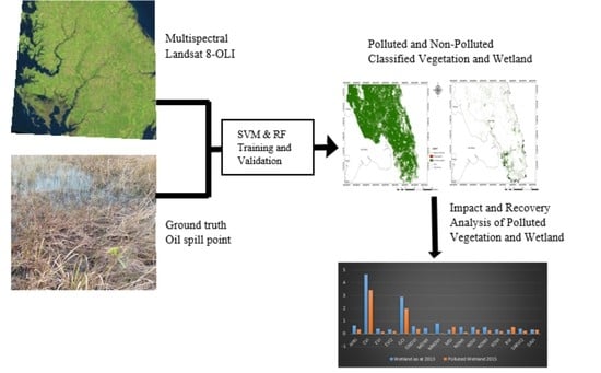
2. Materials and Methods
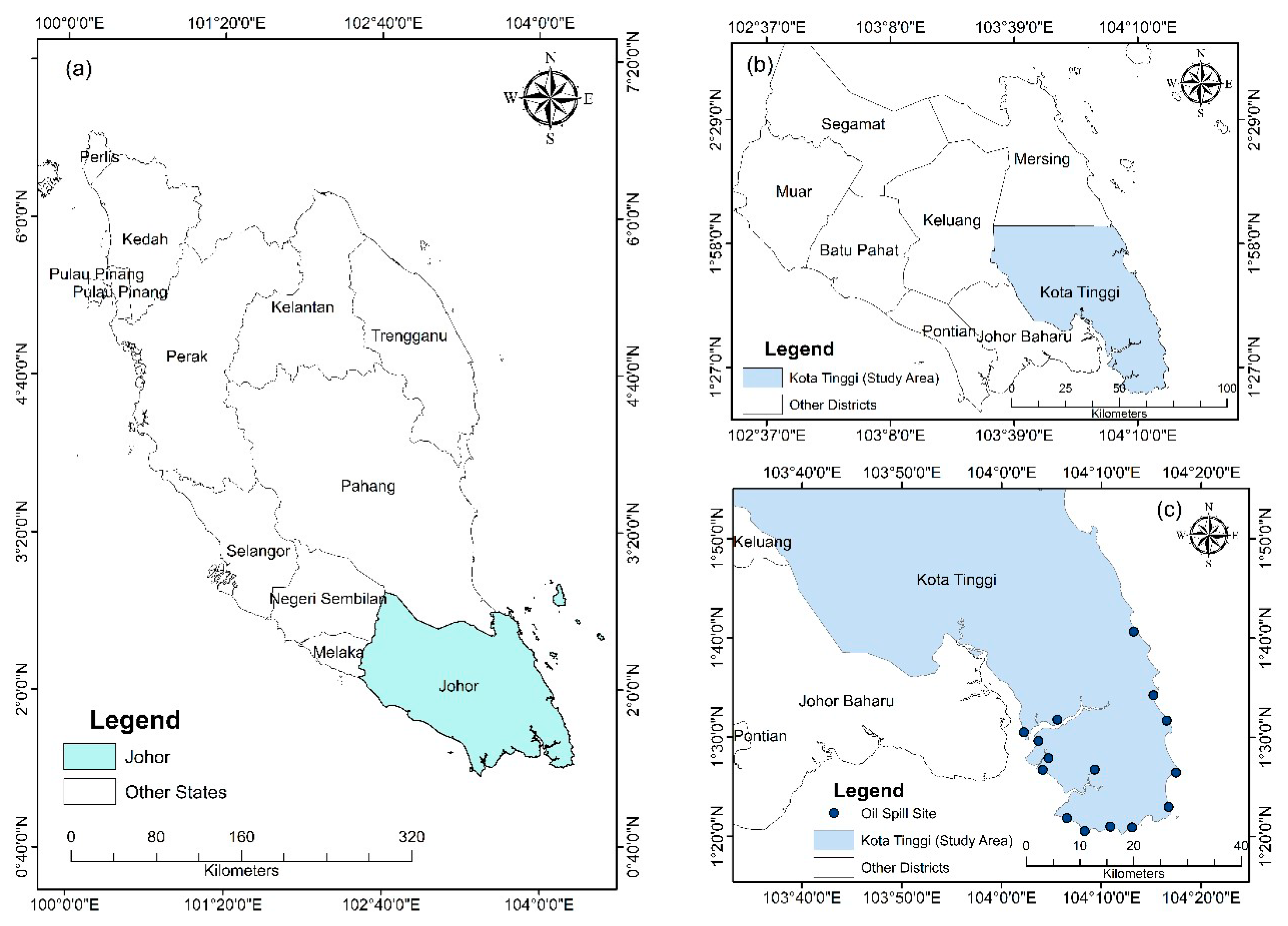
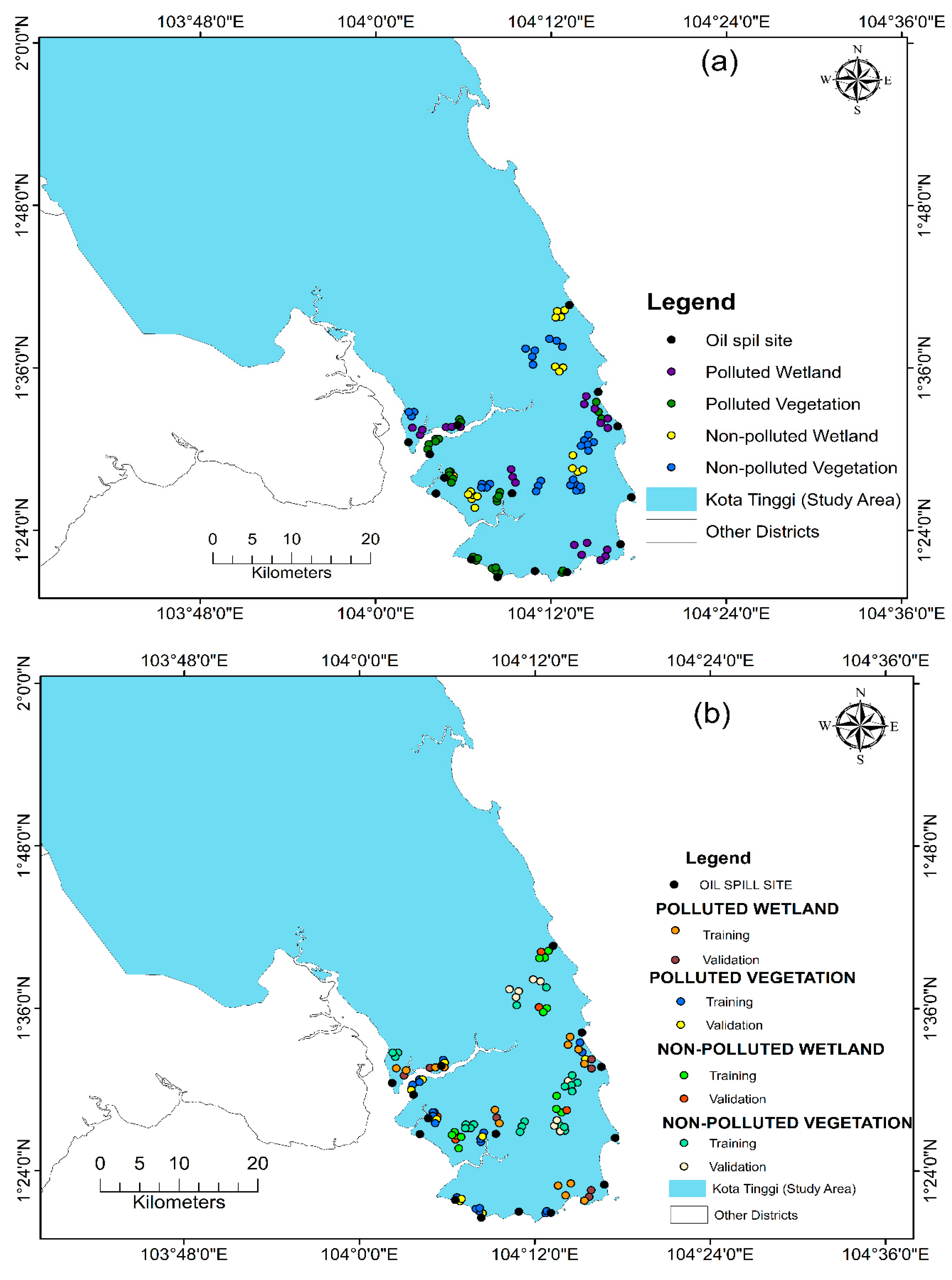
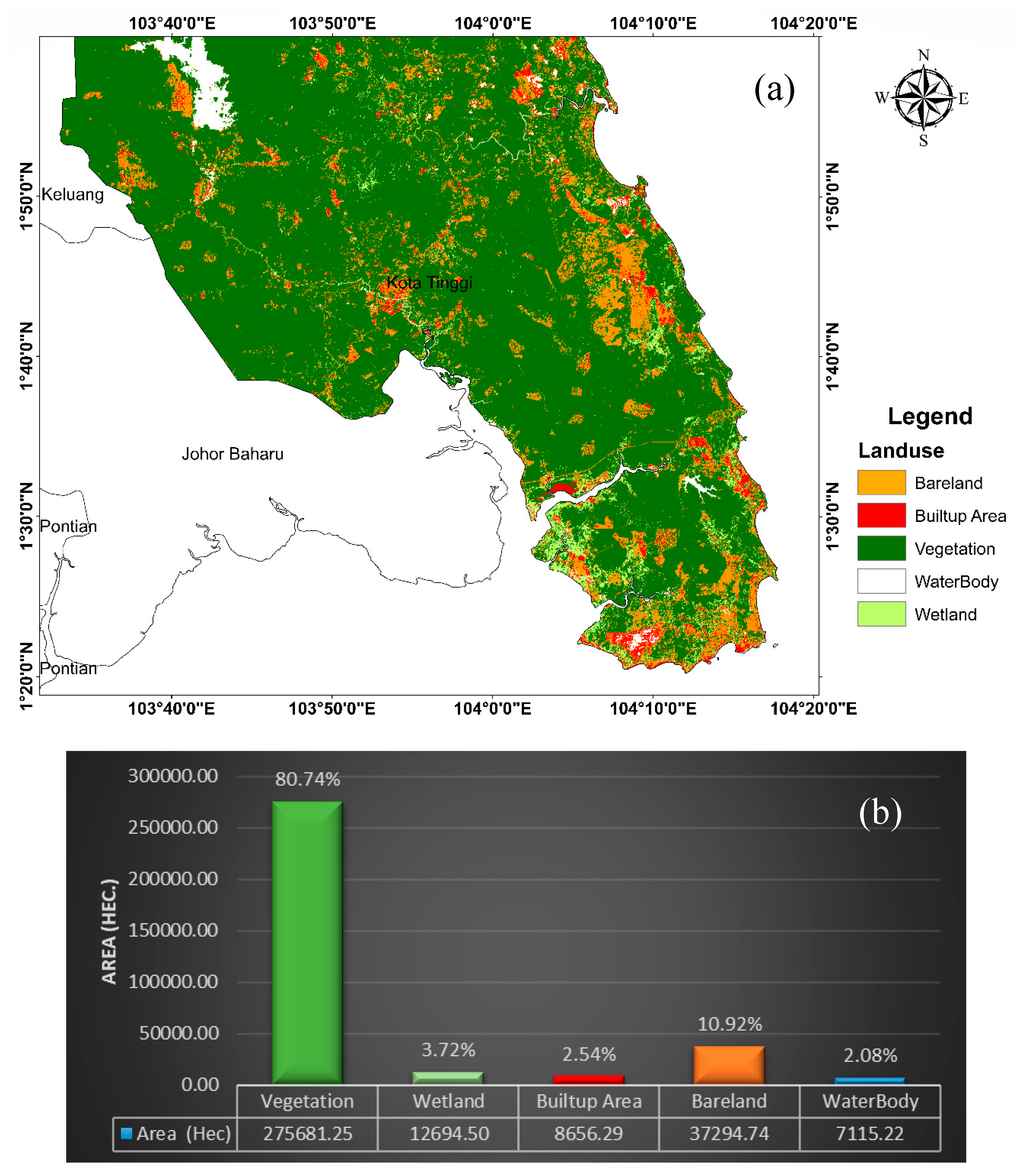
2.1. Study Area

Johor (Figure 1a) is bounded by straits of Malacca in the west, straits of Johor in the south and China Sea in the east. It has a total of 400 km of coastline, majorly in the east and west, which are predominantly habitats of mangrove, swampy wetland, grasses and Niplah forest [44]. High percentage of oil palm production is carried out in Johor because of its fertile land [45], and it is renowned for its intensive port activities, comprising domestic and international marine transportation. The coastal city, especially Kota Tinngi (Figure 1b), is highly vulnerable to oil spills because of the frequent use and movement of petroleum products that are often discharged into the water body [46]. Similarly, its proximity to the China sea, which experiences intense cargo vessel movements, exacerbates its vulnerability to oil spill pollution [47]. This frequent transportation of crude oil has caused different oil spills like the Jeti PML plant vessel explosion and fire (2012), Sungai Kapal sludge oil spill (2012), Nelayan KG diesel spill (2013), Kuantan Port ship collision oil spill (2014), Sungai Kampung Belungkor (2014), Kota Tinggi Johor oil spill (2014), Tg Belungkor Jetty and Kota Tinggi Johor medium fuel spill (2014), contaminating several beaches around Johor’s coastal line [48] and affecting a large expanse of vegetation and wetland (Figure 1c).

2.2. Data Used

The first step in this study was the collection of oil spill data (2014) of the study area from Malaysia’s Ministry of Environment, which includes the location, date, time, causes and the type of spill. These spills, comprising mostly crude oil, heavy fuel, Tarball, medium fuel and diesel, usually originated from ship accidents and pipeline leakages and are subsequently washed to the coastal areas over time, affecting the vegetation and wetland. Within the state of Johor, Kota Tinggi experienced a larger portion of the oil spill, which is attributable to the presence of the Liquid Natural Gas (LNG) terminal at Pangarran and a major ship route at Tanjun Balau and strait of Johor. A total of fifteen sites (See Figure 1c) were identified to have been affected by the oil spill, with a land area of more than 3600 square meters (sqm). Forty-nine ground-truth points were then identified around these oil spill sites (Figure 2a,b), and a buffer area of 60 m was created around the points (Figure 2c) for the classification exercise. As a control point, a total of 54 nonpolluted sites (ground-truth data) with similar 60 m buffer as obtained for the polluted sites were also identified (Table 1). To classify the wetland and vegetation polluted and nonpolluted areas, the ground truth data of the classes were divided into 70% training and 30% validation data.
To undertake the oil spill impact and recovery analysis, a reconnaissance survey was conducted for site selection using Google Earth aerial photographs, which identified Land Use Land Cover (LULC) changes in the study area between 2014 and 2018. Sites with significant infrastructural developments, land reclamation and deforestation were excluded from the analysis, and a total of nine sites were used for the impact and recovery analysis.

2.3. Landsat 8-OLI

Landsat 8-OLI of row and path 59 and 125 between 2013–2018 were acquired from the NASA Landsat mission’s global land cover launched in 2013. Landsat 8 has improved technical features. The NIR band has a closer width to Moderate Resolution Imaging Spectroradiometer (MODIS) near infrared (NIR) band, which is widely used in detection of vegetation health status [7,19]. In addition, two reflectance wavelength bands have been added: the shorter wavelength blue band (0.43–0.45) and shortwave infrared SWIR band (1.36–1.39). The former improves the chlorophyll sensitivity while the latter enables cloud cirrus detection [49,50]. The acquired Landsat 8-OLI (level 2) imageries were from December 2013 to December 2018 during the monsoon period with lesser rainfall and minimal cloud cover. The images with the lowest cloud cover of 20% were acquired and subjected to sun angle atmospheric correction. The Landsat 8-OLI image was re-projected to Universal Transverse Mercator (UTM) in accordance to the study location (Johor, Malaysia). These procedures are pertinent to quality control and assurance since the study depends majorly on the spectral values from the imageries. Table 2 presents the image’s specifications.

2.4. Machine Learning Algorithms

In machine learning, size, number of samples, target variable and training data determine the algorithm selection [39,40]. Specifically, there are mainly 2 types of modeling: supervised and unsupervised learning, which depend on the target availability. There are also 2 main types of results: regression or classification output, which depend on target type, factor or numeric. For this study, two supervised learning classification models (Support Vector Machine (SVM) and Random Forest (RF)) were used.

2.4.1. Support Vector Machine (SVM)

Support vector machine (SVM) is a supervised statistical learning technique developed by Vapnik in 1995 [51,52]. Its applications cut across areas like machine vision, handwriting digit and text identification and satellite imagery classification [53,54]. The model is based on user-defined Kernel function for mapping nonlinear decision boundaries in a dataset to linear boundaries of high-dimensional construct [55] with the goal of ascertaining the hyperplane that optimally separates different classes [56,57]. This hyperplane is determined using training data while validating data set are used for making inference [55]. For this study, both the training and validation data sets are represented by a point vector with a 60 m buffer on the stacked 23 spectral variables (See Table 3). In addition to being a binary classifier, SVMs are also used for multiple class classification through the One Against All and One Against One (OAA and OAO, respectively) [58]. SVM was used for the discrimination of the oil-spill- and non-oil-spill-affected vegetation and wetland in various studies [56,58,59,60].

2.4.2. Random Forest (RF)

Random forest (RF) is a set of tree predictors wherein each tree relies on the value of a random vector sampled independently and with the same distribution for all trees in the forest [61]. Being an ensemble method, random forest is based on the combination of bootstrap aggregation. Individual trees are parameterized through random selection of samples from observations as training data, enabling multicollinearity reduction [62]. RF has been used for the successful classification of oil-spill- and non-oil-spill-affected vegetation and wetland [49,59,63].

2.4.3. Machine Learning Models for Pollution Classification

The evaluation of the 2 machine learning models for the classification and extent quantification were conducted in 2 stages. The first stage involves the stacking of Landsat 8-OLI band 1-7 and 16 spectral vegetation indices as presented in Table 3. The vegetation indices were all derived from the Landsat 8-OLI imagery of December 2014 which is a cloud-free imagery acquired from the US Geological Survey (USGS) website. The training of the two models was subsequently carried out by first conducting the parameterization of the ground truth on the stacked images. The output was then used for the classification of the area into polluted, nonpolluted and others (spectral reflectance for built-up areas and bare land that are not of interest). Upon the completion of the training task, the validation data set was used to assess the reliability of the models using confusion matrix. The training and validation activities were performed using EnMap Box software.

2.5. Accuracy Assessment

Several methods have been developed and used in the assessment of machine learning models for thematic map classifications [64,65], but the error matrix—also referred to as confusion matrix, confusion table or contingency table—is mostly used [40,59,66,67,68]. Error matrix comprises of a square of array values in rows and columns, depicting the number of sampling units of a class to the same class of the verified (validation) ground truth [65,69]. For this study, the evaluation of the accuracy for each of the Machine Learning models were based on a harmonic mean of precision and sensitivity recall (F1 accuracy) and the number of matrices derived from the error matrix based on the 30% validation datasets for the four different classes (polluted vegetation, polluted wetland, nonpolluted vegetation and nonpolluted wetland). F1 accuracy presents the harmonic mean of precision and sensitivity recall which ascertain the out-of-bag error of the model [39]. Equation (1) is used for the F1 accuracy calculation.
F 1   accuracy = 2 P r e c i s i o n R e c a l l R e c a l l + P r e c i s i o n
The Precision is the division of the true positive pixels (TP) by the sum of true positive pixels and false positive (FP) pixels (Equation 2), while the recall is the division of true positive pixels by the sum of true positive pixel and false negative (FN) pixel (Equation (3)).
Precision = T P T P + F P
Recall = T P T P + F N
The matrix values are based on overall accuracy (OA), User’s accuracy (UA) and producers’ accuracy (PA). The OA indicates the percentage or proportion of the overall map which is correctly classified based on the validation ground truth dataset; UA connotes the proportion of a map class (Pixel) that is correctly classified with reference to that particular class (Pixel) on the validation ground truth; and PA is the proportion of a particular class on the ground that is mapped as that particular class, i.e., how well the assigned pixel is classified [68,70]. These are more accurate reliability assessment indices than the Kappa coefficient, which is an overall measure of accuracy based on a random allocation agreement incorporating an adjustment. Although the Kappa statistic is popular, it is not appropriate for accuracy comparison between different models [67,71] because of its inability to distinguish between elements in the confusion matrix [69]. The four accuracy assessment matrices for the two models were computed from the polluted and nonpolluted classification classes and the proportion areas of the four classes where indicated. Finally, the results were evaluated using the Ms Nemar’s chi-square (X2) test to compare them statistically at a confidence level of 95% [72] in order to achieve a marginal homogeneity between the two classes as adopted by [40,59].

2.6. Vegetation Indices

Vegetation indices are defined based on the arithmetic combination of two or more spectral bands from an electromagnetic wave reflectance information acquired through satellites [73]. Variations in the reflectance of light spectra indicate the status of the target plant under study. The effect of oil spill hydrocarbon pollution on wetland and vegetation can be identified through changes in the rate of photosynthesis; changes in the relative and absolute concentration of chlorophyll a and b; changes in lead size; thickness and structure [41,74]. Previous studies have utilized several indices to assess vegetation health status, like eight vegetation indices used in [39], three indices [40], one index [75], and two indices [32]. In this study, we utilized sixteen different indices (Table 4) derived from existing literature to examine the effect and recovery pattern of oil spill polluted vegetation and wetland. The impact was ascertained by comparing the vegetation indices value from the polluted site before and after oil spills. Results from 2013 imagery were used for the pre-oil spill analysis and 2015 for the post-oil-spill assessment.

2.7. Model Hyper-Parameter Optimization

The models were trained and validated using EnMap software [91]. Hyper-parameters’ optimization entails using a set of optimal values as parameters to improve the learning rate, forming an integral part of the general model training. Similar to the approach adopted by [59], the two models were optimized using k-fold (where k = 10) cross-validation by randomized sampling to a certain iteration on the training dataset (Table 5). For SVM, the Gaussian radial basis function (RBF) kernel, which is a multidimensional distribution describing the distance between the input vector and the predefined center vector, has a value of 10; regularization parameter (C) has a value of 10 while the sigma, which represents the weight of the RBF kernel, has a value of 0.001000 on a variable/class number of four. On the other hand, the RF model’s variable/class was four with a tree of 500 and an impurity function of Gini Coefficient.

2.8. Land Use Land Cover (LULC) of the study area

The LULC analysis gives information of the spatial distribution of different land use in a particular area at a point in time [92]. This is important to identify the land use type in the study area, especially the vegetation and wetland. In this study, the land use distribution of the study area for 2014 was analyzed using Random Forest machine learning model and Landsat 8 OLI satellite multispectral imagery of December 2014 because of its low cloud cover. The area is surrounded by water bodies that include the South China Sea, Strait of Johor and some parts of Malacca. Based on the Malaysia Land Area Boundary Administration Map Shape file from (diva-gis.org), the subject site is predominantly made up of four major land uses: vegetation, bare land, built-up area and waterbody. The vegetation is divided into terrestrial vegetation and wetland (swampy area). From Figure 3a,b, a higher percentage of the area (80.74%; 275,681.25 hectares) is made up of vegetation. Next to that is bareland, with 10.92% (7115.22 hectares), wetland 3.72% (12,694.50 hectares) and builtup area 2.54% (8656.29 Hectares). The overall accuracy from the model classification and validation was 99.83%, with a standard error of 0.03%, confirming the model’s high accuracy.

3. Results and Discussion

3.1. Accuracy Assessment

The F1, OA, PA and UA error matrix values for the four categories (polluted vegetation, polluted wetland, nonpolluted vegetation, nonpolluted wetland) classification from SVM and RF were used for the accuracy assessment as shown in Table 6 and Table 7. While the former represents the result for the study area alone, the latter shows the performance of similar training and validation data set in classifying larger areas by including Pontian, Johor Baharu and part of Keluang. All the training and validation datasets for this study were the same for both models. The assessment results for the study area reveal that RF outperforms SVM, with F1 (95.32%), OA (96.80%), UA (98.82%) and PA (95.11%) as against the SVM’s accuracy values of F1 (80.83%), OA (92.87%), PA (95.18%) and UA (93.81%), respectively.
It can also be seen from the PA that the classification of nonpolluted vegetation has a high accuracy for both SVM and RF. For the UA, nonpolluted vegetation has a higher accuracy in SVM, while the polluted wetland has the highest for RF. Assessing the models’ performance on a larger area, the RF outperformed the SVM with F1 (85.56%), OA (86.31%), PA (88.29%), and UA (95.45%) compared to the SVM’s 80.31%, 83.61%, 89.17% and 90.67%, respectively. This reveals a similar performance pattern irrespective of the size of the study area. However, the models’ accuracies in the larger area were lower than those of the smaller study area. This is likely due to the smaller number of the data sets used in this regard [39]. Analysis of the McNemar’s chi-squared (X2) (Table 8) indicates significant statistical differences across the four classification groups in the two models for the study area. (p < 0.05) implies significant statistical difference in the area classification of each of the categories.

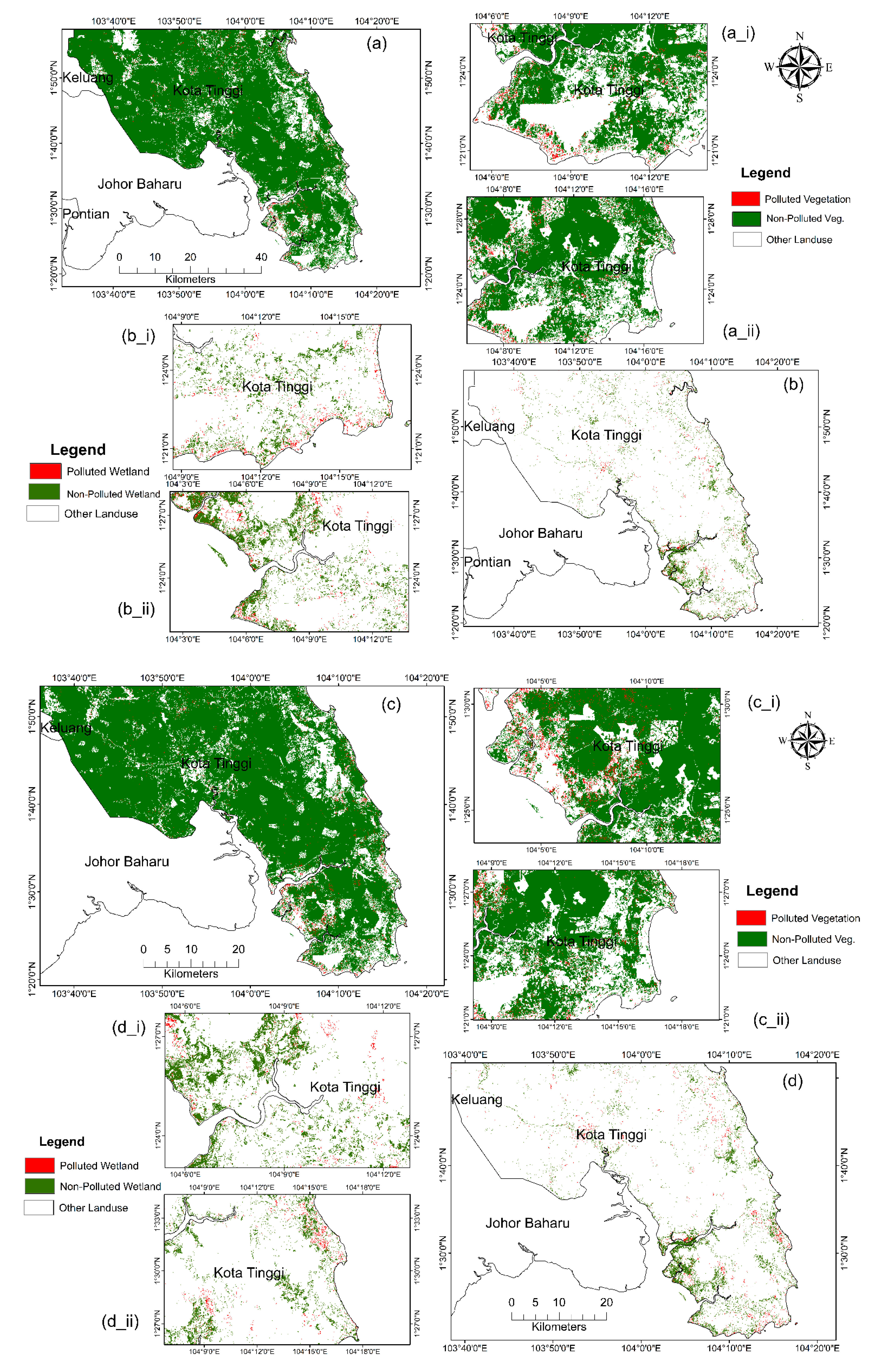
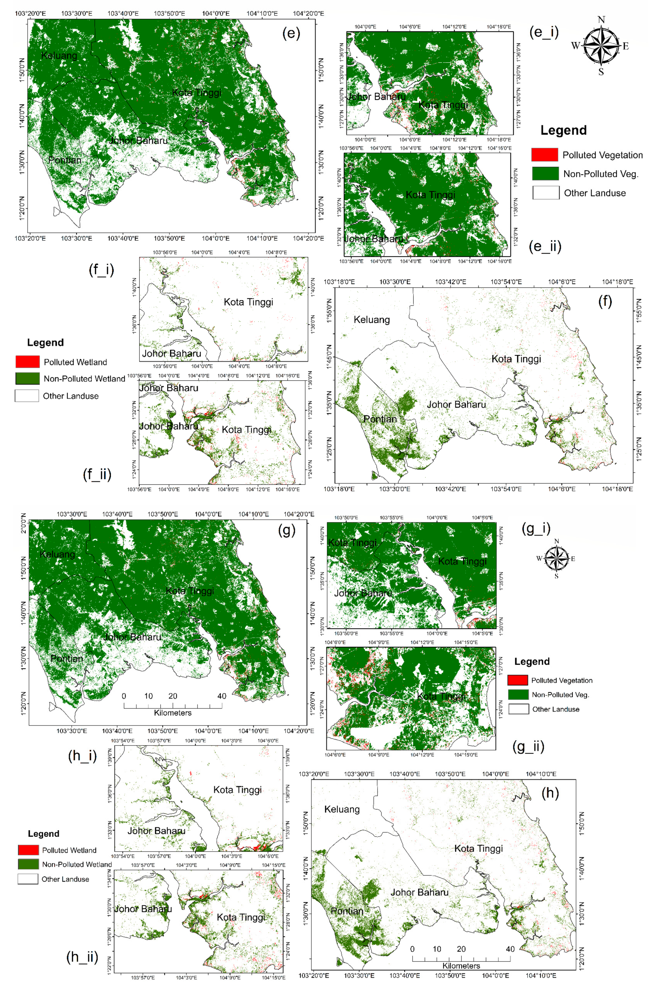
3.2. Classification and Mapping of Polluted Coastal Areas (Vegetation and Wetland)

Figure 4a–i shows the models’ classification outcomes. The SVM classification for the four classes (polluted vegetation, polluted wetland, nonpolluted vegetation, nonpolluted wetland) are presented in Figure 4a,b while Figure 4c,d shows the classification maps from the RF model for the main study area. Figure 4i indicates variations in the models’ area classification. For instance, slight differences in the output area for similar classes in the two models exist across the four classes. The areas of polluted vegetation and polluted wetland in SVM are higher than those of RF, while nonpolluted vegetation and nonpolluted wetland areas are higher for RF than SVM. Based on the RF model, the polluted vegetation and the nonpolluted vegetation areas are 2949.79 hectares and 272,731.46 hectares, respectively, while the SVM classified the polluted vegetation and nonpolluted vegetation at 3004.93 hectares and 272,676.32 hectares, respectively, revealing a difference of 55.14 hectares each for the polluted and nonpolluted vegetation areas. It can be inferred that the lower accuracy of the SVM model affects its ability to adequately classify the entire area [39,59]. Similarly, in the classification of wetlands (polluted and nonpolluted), the polluted wetland areas are 1205.98 hectares and 1209.79 hectares from the RF and SVM models respectively. For nonpolluted wetland, RF classification is 11,488.52 hectares, and SVM classification is 11,484.71 hectares, revealing a difference of 3.81 hectares in both instances. Field observations using some purposively selected sites show that RF models have a high true positive accuracy for the four classification categories than SVM, which is reflected in the higher classification accuracy of RF polluted and nonpolluted area extents in comparison to the SVM’s.

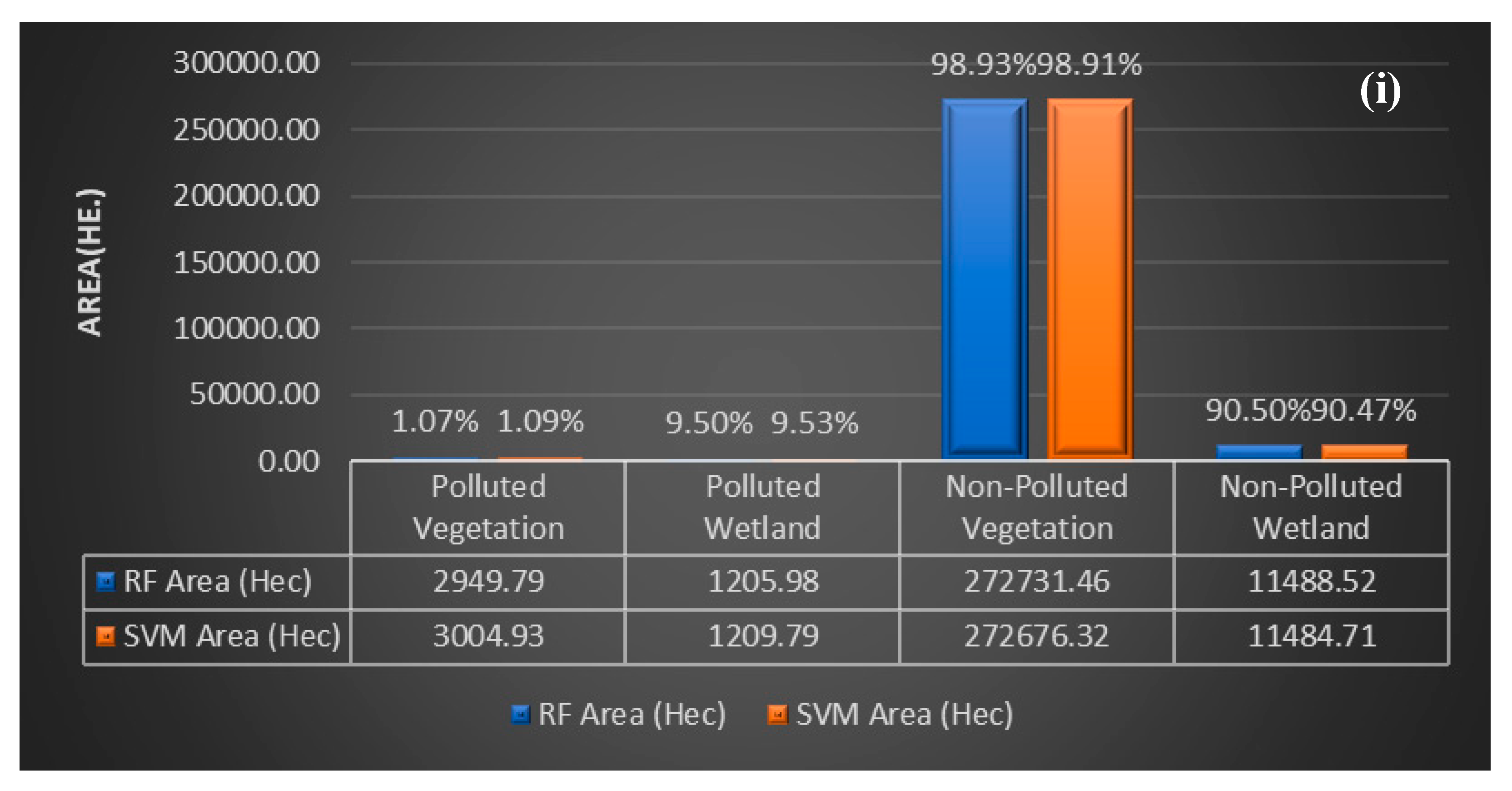
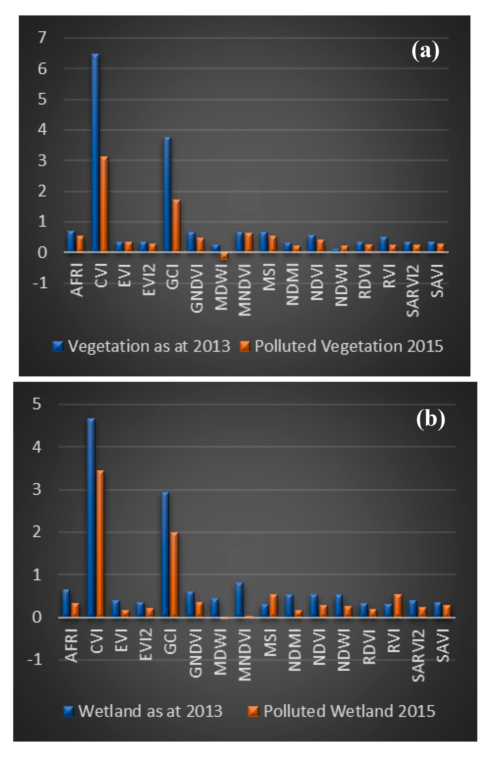
3.3. Oil Spill Pollution Impact Assessment on Vegetation and Wetland

The impact of oil spill on affected vegetation and wetland was examined using the sixteen vegetation indices presented in Table 4. These indices can provide information on the wetland and vegetation health stress due to the oil spill [32,33,39]. The vegetation indices of 2013 were used for pre-oil-spill assessment, while 2015 indices were used for post-oil-spill assessment of the polluted vegetation and wetlands. As depicted in Figure 5a, the comparison of the pre- and post-oil-spill status of the vegetation area showed a general decrease in vegetation health with respect to 15 of the indices. However, the NDWI after oil pollution shows an increase in value, which is likely due to the high absorption and presence of surface water that changed over time [63,93]. Further analysis with the use of paired T-Test (Table 9) indicated that nine of the fifteen indices that reflect deterioration in post oil spill vegetation health (RVI, CVI, GCI, GNDVI, NDVI, MSI, MDWI, SARVI2 and SAVI) were statistically significant with p-value < 0.05. Similarly, from Figure 5b, which represents differences between the pre- and post-oil-spill impact on wetland, a general reduction in the values of all the wetland assessment indices was observed. However, MSI and RVI increased in 2015, two years after contact with oil hydrocarbons. Figure 6 shows the weight of the indices in classifying oil spill impacts in the study area. For the SVM model, a high percentage of the indices (variables) showed significant contributions, with the first five variables, SARVI2, AFRI, NIR, NDVI and MSI, being the most sensitive to oil spills in the study area. In contrast, CVI, Blue, Green, SWIR-1 and GCI, showed more sensitivity in the RF model.
Analysis of these outcomes indicates that an overwhelming majority of the assessment indices respond negatively to exposure to hydrocarbon, with a T-test statistical significance level (p-value) < 0.05. Further, it is observable that wetlands are more impacted by oil spills than vegetation due to their closeness to the waterbody. A higher percentage of the polluted sites are located at the south, southeast and southwest regions of the study area. However, some polluted sites were equally identified towards the eastern and northern parts of the area. The concentration of the polluted sites in these regions is due to the higher number of oil spills recorded along this area. Moreover, the limited detection of polluted sites in the eastern and northern regions is likely due to the undocumented terrestrial oil spill incidents that have occurred along that axis, which has limited the scope of this study. To date, a significant number of oil spill incidents are not well-documented [94].
Based on the foregoing, we conclude that vegetation indices are suitable proxies for estimating the effects of hydrocarbon spill on vegetation as well as wetland. This is similar to the findings of [32,33,35,39,40] wherein vegetation indices were used to examine the effect of the oil spill on vegetation. Although the focus of those studies was terrestrial vegetation, this present study has shown that the approach can also be extended to wetland assessment. Moreover, aside from the common indices (CVI, GCI, GNDVI, NDVI, MDWI, SARVI2 and SAVI), which show a significant deterioration in both polluted vegetation and wetland, EVI, EVI 2, MNDVI, NDMI, NDWI and RDVI can also be used for detecting the effect of the oil spill on wetland. From evaluating the p-value (Table 9), it is evident that CVI, MDWI, NDVI and GCI are more significant in the assessment of both vegetation and wetland oil spill impacts, in addition to MNDVI for wetland assessment.

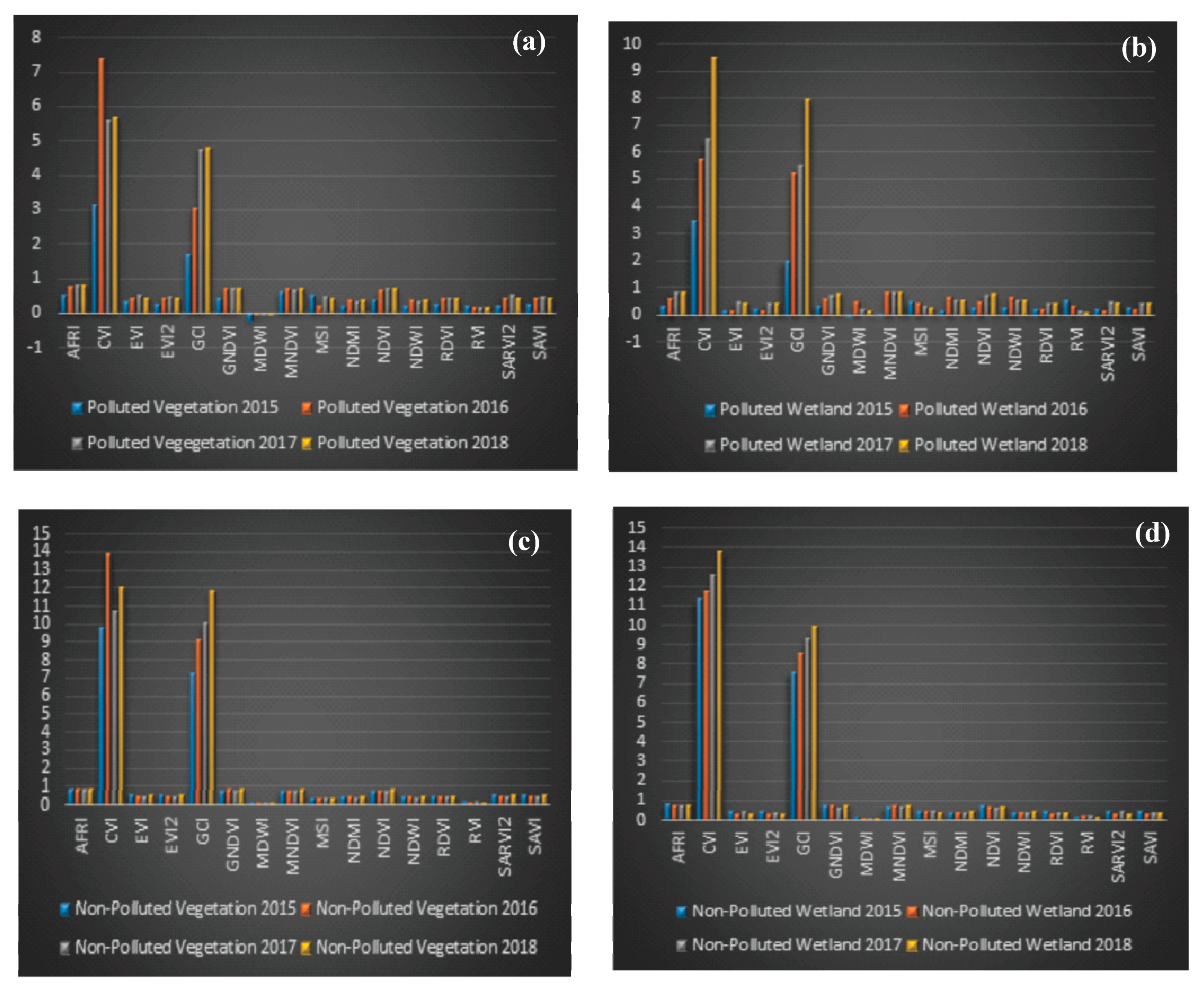
3.4. Polluted Vegetation and Wetland Recovery Assessment

The effects of oil spills cover the broad range of vegetation loss caused by reduction of plant chlorosis, loss of water and soil moisture level reduction, among others [95]. Over the years, this has been the scenario of the affected oil spill sites in the study area. The recovery assessment of the affected vegetation and wetland areas was based on the comparison with nonaffected areas from 2015 to 2018. Figure 7a shows the vegetation recovery pattern which is based on all the sixteen indices, with emphasis on nine of the vegetation indices (RVI, CVI, GSI, GNDVI, NDVI, MSI, MDWI, SARVI2 and SAVI). The choice of these indices is premised on their ability to depict the effect of the oil spill on vegetation, as discussed in Section 3.3. Figure 7a highlights the significant improvement in the vegetation health exemplified by enhanced greenness through chlorosis, leaf water retention and soil moisture level increment. This is represented by the increase in the values of most of the indices after the oil spill, which is attributable to the various treatment that the vegetation was subjected to during this period. Similarly, the recovery of the wetland (Figure 7b) was assessed based on the fourteen vegetation indices discussed in Section 3.3. The observed recovery across all the vegetation indices aligns with the findings of [15,19] that depicted vegetation recovery sometime after exposure to the oil spill.
For further insights, the status of the nonpolluted vegetation and nonpolluted wetland was also evaluated over a similar period (Figure 7c,d). Comparing Figure 7a (polluted vegetation) and Figure 7c (nonpolluted vegetation), it is seen that the indices in the nonpolluted area have higher values than the polluted area, reflecting noticeable changes in the status of the polluted vegetation. A similar pattern is seen in the polluted wetland and nonpolluted wetland in Figure 7b,d.

4. Conclusions

This study has evaluated the potential of multispectral Landsat 8-OLI remote sensing satellite imagery and machine learning models in the quantification of pollution extent through the classification of oil-spill-polluted vegetation and wetland. Advancing previous studies that have focused on monitoring terrestrial vegetation, we evaluated oil spill impacts on wetlands in addition to vegetation. Further, we undertook a systematic assessment of the recovery of the affected zones, which has been sparsely addressed in earlier studies. Support Vector Machine (SVM) and Random Forest (RF) machine learning models were used in the discrimination of the polluted and nonpolluted vegetation and wetland. The accuracies of the two models were validated using four parameters: F1, OA, UA and PA, with the RF outperforming the SVM across the board. McNemar’s chi-squared (X2) analysis indicated a statistically significant difference in the proportion of land area classification covered by the four (polluted wetland and vegetation, nonpolluted wetland and vegetation as represented in Figure 4i) with p-value < 0.05 from the two models.
Sixteen vegetation health indices were used for the assessment of the impacts of oil spills on vegetation and wetland over a two-year period (2013–2015) which represent pre-oil-spill (2013) and post-oil-spill (2015). Analysis of the results indicates significant vegetation and wetland stress. As observed from the result of the vegetation, 93% of the indices reflected a reduction in value but only 56% were statistically significant at p-value < 0.05. For the wetland, 87.5% of the indices showed a reduction in value of pre- and post-oil-spill sites and are all statistically significant at p-value < 0.05.
CVI, MDWI, NDVI, GCI, GNDVI, SARVI2 and SAVI are appropriate for both vegetation and wetland impact assessment, with the first four being the most suitable because of their higher significance level in indicating plant stress in comparison to other indices. In addition to these seven homogenous indices, EVI, EVI 2, MNDVI, NDMI, NDWI and RDVI can also be used to examine wetland hydrocarbon oil spill impact since the greenness of vegetation and sensitivity to high biomass region are most represented by the NIR, SWIR and RED bands which are the basis of the indices.
In addition, the comparison of the nonpolluted and polluted areas over a similar period confirmed the healthier status of the former, although signs of recovery were observed in the latter, which is likely due to treatment interventions by the government. However, more initiatives are required to improve the recovery process. In conclusion, it can be inferred that remote sensing technology and machine learning models are powerful and reliable tools for the impact and recovery assessment of oil-spill-affected vegetation and wetland.

Author Contributions

Conceptualization, A.-L.B. and S.T.Y.; methodology, S.T.Y.; software, S.T.Y.; validation, A.-L.B., S.T.Y., B.P. and O.F.A.; formal analysis, A.-L.B. and S.T.Y.; investigation, A.-L.B. and S.T.Y.; resources, A.-L.B.; data curation, S.T.Y.; writing—original draft preparation, S.T.Y.; writing—review and editing, A.-L.B., S.T.Y., B.P. and O.F.A.; visualization, B.P. and O.F.A.; supervision, A.-L.B.; project administration, A.-L.B., B.P., O.F.A.; funding acquisition, A.-L.B. All authors have read and agreed to the published version of the manuscript.

Funding

This research was funded by the University Teknologi PETRONAS (UTP) Y-UTP Research Project Grant (015LC0-003).

Acknowledgments

This study will like to acknowledge the University Teknologi PETRONAS (UTP) Y-UTP Research Project Grant (015LC0-003); Malaysia Ministry of Environment (Jabatan Alam Sekitar) for providing oil spill location data; the U.S. Geological Survey (USGS) for making Landsat 8 OLI multispectral imageries freely available; Earth Resources Observation and Science (EROS) Center and the German Hyperspectral Satellite Mission for providing the open-source EnMap software; QGIS Development Team for providing free QGIS Software. The anonymous reviewers for their constructive comments and impactful contributions to the manuscript.

Conflicts of Interest

The authors declare no conflict of interest.

References

  1. Statham, P.J. Nutrients in estuaries—An overview and the potential impacts of climate change. Sci. Total. Environ. 2012, 434, 213–227. [Google Scholar] [CrossRef]
  2. Halpern, B.S.; Frazier, M.; Potapenko, J.; Casey, K.S.; Koenig, K.; Longo, C.; Lowndes, J.S.; Rockwood, R.C.; Selig, E.R.; Selkoe, K.A.; et al. Spatial and temporal changes in cumulative human impacts on the world’s ocean. J. Nat. Commun. 2015, 6, 7615. [Google Scholar] [CrossRef] [PubMed] [Green Version]
  3. Menicagli, V.; Balestri, E.; Vallerini, F.; Castelli, A.; Lardicci, C. Adverse effects of non-biodegradable and compostable plastic bags on the establishment of coastal dune vegetation: First experimental evidences. Environ. Pollut. 2019, 252, 188–195. [Google Scholar] [CrossRef] [PubMed]
  4. Ferreira, A.M.; Marques, J.C.; Seixas, S. Integrating marine ecosystem conservation and ecosystems services economic valuation: Implications for coastal zones governance. Ecol. Indic. 2017, 77, 114–122. [Google Scholar] [CrossRef] [Green Version]
  5. Zhang, H. Transport of microplastics in coastal seas. Estuarine, Coast. Shelf Sci. 2017, 199, 74–86. [Google Scholar] [CrossRef]
  6. Yekeen, S.; Balogun, A.; Aina, Y. Early Warning Systems and Geospatial Tools: Managing Disasters for Urban Sustainability. In Sustainable Cities and Communities; Filho, W.L., Azul, A.M., Brandli, L., Özuyar, P.G., Wall, T., Eds.; Springer International Publishing: Berlin/Heidelberg, Germany, 2019; pp. 1–13. [Google Scholar]
  7. Rocha, F.; Homem, V.; Castro-Jiménez, J.; Ratola, N. Marine vegetation analysis for the determination of volatile methylsiloxanes in coastal areas. Sci. Total. Environ. 2019, 650, 2364–2373. [Google Scholar] [CrossRef] [Green Version]
  8. Li, P.; Cai, Q.; Lin, W.; Chen, B.; Zhang, B. Offshore oil spill response practices and emerging challenges. Mar. Pollut. Bull. 2016, 110, 6–27. [Google Scholar] [CrossRef]
  9. Balogun, A.-L.; Matori, A.-N.; Kiak, K.W.T. Developing an emergency response model for offshore oil spill disaster management using spatial decision support system (sdss). ISPRS Ann. Photogramm. Remote. Sens. Spat. Inf. Sci. 2018, 4, 21–27. [Google Scholar] [CrossRef] [Green Version]
  10. Lynch, L.E. Statement by Attorney General Loretta E. Lynch on the Agreement in Principle with BP to Settle Civil Claims for the Deepwater Horizon Oil Spill. 31 March 2015. Available online: https://www.justice.gov/opa/pr/statement-attorney-general-loretta-e-lynch-agreement-principle-bp-settle-civil-claims (accessed on 29 December 2019).
  11. Ndimele, P.E.; Saba, A.O.; Ojo, D.O.; Ndimele, C.C.; Anetekhai, M.A.; Erondu, E.S. Remediation of Crude Oil Spillage. In The Political Ecology of Oil and Gas Activities in the Nigerian Aquatic Ecosystem; Elsevier: Amsterdam, The Netherlands, 2018; pp. 369–384. [Google Scholar]
  12. Angelova, D.; Uzunov, I.; Uzunova, S.; Gigova, A.; Minchev, L. Kinetics of oil and oil products adsorption by carbonized rice husks. Chem. Eng. J. 2011, 172, 306–311. [Google Scholar] [CrossRef]
  13. De la Huz, R.; Lastra, M.; López, J. Other Environmental Health Issues: Oil Spill. In Reference Module in Earth Systems and Environmental Sciences; Academic Press: Amsterdam, The Netherlands, 2018. [Google Scholar]
  14. Jana, A.; Maiti, S.; Biswas, A. Seasonal change monitoring and mapping of coastal vegetation types along Midnapur-Balasore Coast, Bay of Bengal using multi-temporal landsat data. Model. Earth Syst. Environ. 2015, 2, 7. [Google Scholar] [CrossRef] [Green Version]
  15. Mendelssohn, I.A.; Andersen, G.; Baltz, D.M.; Caffey, R.H.; Carman, K.R.; Fleeger, J.W.; Joye, S.; Lin, Q.; Maltby, E.; Overton, E.B.; et al. Oil Impacts on Coastal Wetlands: Implications for the Mississippi River Delta Ecosystem after the Deepwater Horizon Oil Spill. BioScience 2012, 62, 562–574. [Google Scholar] [CrossRef]
  16. Lin, Q.; Mendelssohn, I.A. Impacts and Recovery of the Deepwater Horizon Oil Spill on Vegetation Structure and Function of Coastal Salt Marshes in the Northern Gulf of Mexico. Environ. Sci. Technol. 2012, 46, 3737–3743. [Google Scholar] [CrossRef] [PubMed]
  17. Duke, N.; Pinzón, M.Z.S.; Prada, T.M.C. Large-Scale Damage to Mangrove Forests Following Two Large Oil Spills in Panama1. Biotropica 1997, 29, 2–14. [Google Scholar] [CrossRef]
  18. Sheppard, C.R. Regional Chapters: Europe, The Americas and West Africa. In Seas at the Millennium: An Environmental Evaluation; Academic Press: Amsterdam, The Netherlands, 2018. [Google Scholar]
  19. Jackson, J.B.C.; Cubit, J.D.; Keller, B.D.; Batista, V.; Burns, K.; Caffey, H.M.; Caldwell, R.L.; Garrity, S.D.; Getter, C.D.; Gonzalez, C.; et al. Ecological Effects of a Major Oil Spill on Panamanian Coastal Marine Communities. Science 1989, 243, 37–44. [Google Scholar] [CrossRef]
  20. Pavanelli, D.D.; Loch, C. Mangrove spectra changes induced by oil spills monitored by image differencing of normalised indices: Tools to assist delimitation of impacted areas. Remote. Sens. Appl. Soc. Environ. 2018, 12, 78–88. [Google Scholar] [CrossRef]
  21. Zengel, S.; Weaver, J.; Wilder, S.L.; Dauzat, J.; Sanfilippo, C.; Miles, M.S.; Jellison, K.; Doelling, P.; Davis, A.; Fortier, B.K.; et al. Vegetation recovery in an oil-impacted and burned Phragmites australis tidal freshwater marsh. Sci. Total. Environ. 2018, 612, 231–237. [Google Scholar] [CrossRef]
  22. Delaune, R.D.; Wright, A.L. Projected Impact of Deepwater Horizon Oil Spill on U.S. Gulf Coast Wetlands. Soil Sci. Soc. Am. J. 2011, 75, 1602–1612. [Google Scholar] [CrossRef] [Green Version]
  23. Beyer, J.; Trannum, H.C.; Bakke, T.; Hodson, P.V.; Collier, T.K. Environmental effects of the Deepwater Horizon oil spill: A review. Mar. Pollut. Bull. 2016, 110, 28–51. [Google Scholar] [CrossRef] [Green Version]
  24. Chatterjee, B.; Porwal, M.; Hussin, Y. Assessment of tsunami damage to mangrove in India using remote sensing and GIS. In Proceedings of the XXI ISPRS Congress, Beijing, China, 3–11 July 2008. [Google Scholar]
  25. Jana, A.; Biswas, A.; Maiti, S.; Bhattacharya, A.K. Shoreline changes in response to sea level rise along Digha Coast, Eastern India: An analytical approach of remote sensing, GIS and statistical techniques. J. Coast. Conserv. 2013, 18, 145–155. [Google Scholar] [CrossRef]
  26. Reddy, C.S.; Roy, A. Assessment of Three Decade Vegetation Dynamics in Mangroves of Godavari Delta, India Using Multi-Temporal Satellite Data and GIS. Res. J. Environ. Sci. 2008, 2, 108–115. [Google Scholar]
  27. Fingas, M.; Brown, C. Review of oil spill remote sensing. Mar. Pollut. Bull. 2014, 83, 9–23. [Google Scholar] [CrossRef] [PubMed] [Green Version]
  28. Fan, J.; Zhang, F.; Zhao, D.; Wang, J. Oil Spill Monitoring Based on SAR Remote Sensing Imagery. Aquat. Procedia 2015, 3, 112–118. [Google Scholar] [CrossRef]
  29. Kokaly, R.; Couvillion, B.R.; Holloway, J.M.; Roberts, D.A.; Ustin, S.L.; Peterson, S.; Khanna, S.; Piazza, S.C. Spectroscopic remote sensing of the distribution and persistence of oil from the Deepwater Horizon spill in Barataria Bay marshes. Remote. Sens. Environ. 2013, 129, 210–230. [Google Scholar] [CrossRef] [Green Version]
  30. Khanna, S.; Santos, M.J.; Ustin, S.L.; Shapiro, K.; Haverkamp, P.J.; Lay, M. Comparing the Potential of Multispectral and Hyperspectral Data for Monitoring Oil Spill Impact. Sensors 2018, 18, 558. [Google Scholar] [CrossRef] [PubMed] [Green Version]
  31. Rodgers, J.C.; Murrah, A.W.; Cooke, W.H. The Impact of Hurricane Katrina on the Coastal Vegetation of the Weeks Bay Reserve, Alabama from NDVI Data. Chesap. Sci. 2009, 32, 496–507. [Google Scholar] [CrossRef]
  32. Adamu, B.; Tansey, K.; Ogutu, B. An investigation into the factors influencing the detectability of oil spills using spectral indices in an oil-polluted environment. Int. J. Remote. Sens. 2016, 37, 2338–2357. [Google Scholar] [CrossRef] [Green Version]
  33. Adamu, B.; Tansey, K.; Ogutu, B. Remote sensing for detection and monitoring of vegetation affected by oil spills. Int. J. Remote. Sens. 2018, 39, 3628–3645. [Google Scholar] [CrossRef] [Green Version]
  34. Li, L.; Ustin, S.L.; Lay, M. Application of AVIRIS data in detection of oil-induced vegetation stress and cover change at Jornada, New Mexico. Remote. Sens. Environ. 2005, 94, 1–16. [Google Scholar] [CrossRef]
  35. Adamu, B.; Tansey, K.; Ogutu, B. Using vegetation spectral indices to detect oil pollution in the Niger Delta. Remote. Sens. Lett. 2015, 6, 145–154. [Google Scholar] [CrossRef] [Green Version]
  36. Alam, M.S.; Sidike, P.; Alam, S. Trends in oil spill detection via hyperspectral imaging. In Proceedings of the 2012 7th International Conference on Electrical and Computer Engineering, Dhaka, Bangladesh, 20–22 December 2012; pp. 858–862. [Google Scholar]
  37. Dabbiru, L.; Samiappan, S.; Nobrega, R.A.A.; Aanstoos, J.A.; Younan, N.H.; Moorhead, R.J. Fusion of synthetic aperture radar and hyperspectral imagery to detect impacts of oil spill in Gulf of Mexico. In Proceedings of the 2015 IEEE International Geoscience and Remote Sensing Symposium (IGARSS), Milan, Italy, 26–31 July 2015; pp. 1901–1904. [Google Scholar]
  38. Hese, S.; Schmullius, C. High spatial resolution image object classification for terrestrial oil spill contamination mapping in West Siberia. Int. J. Appl. Earth Obs. Geoinf. 2009, 11, 130–141. [Google Scholar] [CrossRef]
  39. Ozigis, M.S.; Kaduk, J.; Jarvis, C.H. Mapping terrestrial oil spill impact using machine learning random forest and Landsat 8 OLI imagery: A case site within the Niger Delta region of Nigeria. Environ. Sci. Pollut. Res. 2018, 26, 3621–3635. [Google Scholar] [CrossRef] [PubMed] [Green Version]
  40. Ozigis, M.S.; Kaduk, J.D.; Jarvis, C.H.; Bispo, P.D.C.; Balzter, H. Detection of oil pollution impacts on vegetation using multifrequency SAR, multispectral images with fuzzy forest and random forest methods. Environ. Pollut. 2019, 256, 113360. [Google Scholar] [CrossRef] [PubMed]
  41. Arellano, P.; Tansey, K.; Balzter, H.; Boyd, D.S. Detecting the effects of hydrocarbon pollution in the Amazon forest using hyperspectral satellite images. Environ. Pollut. 2015, 205, 225–239. [Google Scholar] [CrossRef] [PubMed]
  42. Sun, R.; Chen, S.; Su, H.; Mi, C.; Jin, N. The Effect of NDVI Time Series Density Derived from Spatiotemporal Fusion of Multisource Remote Sensing Data on Crop Classification Accuracy. ISPRS Int. J. Geo-Information 2019, 8, 502. [Google Scholar] [CrossRef] [Green Version]
  43. Chen, N.; Shi, Y.; Huang, W.; Zhang, J.; Wu, K. Mapping wheat rust based on high spatial resolution satellite imagery. Comput. Electron. Agric. 2018, 152, 109–116. [Google Scholar] [CrossRef]
  44. Karim, S.A.; Rahman, Y.A.; Abdullah, M.J. Management of Mangrove Forests in Johor-as Part of the Coastal Ecosystem Management. In Proceedings of the 2004, Seminar Sumberjaya Pinggir Pantai dan Pelancongan: Isu dan Cabaran, Bukit Merah Laketown Resort, Perak, Malaysia, 20–21 December 2004. [Google Scholar]
  45. Tan, M.L.; Ibrahim, A.L.; Yusop, Z.; Duan, Z.; Ling, L. Impacts of land-use and climate variability on hydrological components in the Johor River basin, Malaysia. Hydrol. Sci. J. 2015, 60, 1–17. [Google Scholar] [CrossRef]
  46. Sakari, M.; Zakaria, M.P.; Mohamed, C.A.R.; Lajis, N.H.; Chandru, K.; Bahry, P.S.; Mokhtar, M.B.; Shahbazi, A. Urban vs. Marine Based Oil Pollution in the Strait of Johor, Malaysia: A Century Record. Soil Sediment Contam. Int. J. 2010, 19, 644–666. [Google Scholar] [CrossRef]
  47. Nagarajan, R.; Jonathan, M.; Roy, P.D.; Wai-Hwa, L.; Prasanna, M.; Sarkar, S.; Navarrete-Lopez, M. Metal concentrations in sediments from tourist beaches of Miri City, Sarawak, Malaysia (Borneo Island). Mar. Pollut. Bull. 2013, 73, 369–373. [Google Scholar] [CrossRef] [Green Version]
  48. Minton, G.; Poh, A.N.Z.; Peter, C.; Porter, L.; Kreb, D. Indo-Pacific Humpback Dolphins in Borneo. In Advances in Marine Biology; Elsevier: Amsterdam, The Netherlands, 2016; Volume 73, pp. 141–156. [Google Scholar]
  49. Roy, D.; Wulder, M.A.; Loveland, T.; Woodcock, C.E.; Allen, R.; Anderson, M.C.; Helder, D.; Irons, J.; Johnson, D.; Kennedy, R.; et al. Landsat-8: Science and product vision for terrestrial global change research. Remote. Sens. Environ. 2014, 145, 154–172. [Google Scholar] [CrossRef] [Green Version]
  50. Shao, Z.; Cai, J.; Fu, P.; Hu, L.; Liu, T. Deep learning-based fusion of Landsat-8 and Sentinel-2 images for a harmonized surface reflectance product. Remote. Sens. Environ. 2019, 235, 111425. [Google Scholar] [CrossRef]
  51. Vapnik, V. The Nature of Statistical Learning Theory; Springer science & business media: Berlin/Heidelberg, Germany, 2013. [Google Scholar]
  52. Cherkassky, V. The Nature Of Statistical Learning Theory. IEEE Trans. Neural Networks 1997, 8, 1564. [Google Scholar] [CrossRef] [PubMed] [Green Version]
  53. Anthony, G.; Gregg, H.; Tshilidzi, M. Image Classification Using SVMs: One-against-One Vs One-against-All arXiv 2007, arXiv:0711.2914. Available online: https://arxiv.org/abs/0711.2914 (accessed on 5 January 2020).
  54. Burges, C.J. A Tutorial on Support Vector Machines for Pattern Recognition. Data Min. Knowl. Discov. 1998, 2, 121–167. [Google Scholar] [CrossRef]
  55. Srivastava, P.K.; Yang, Q.; Rico-Ramirez, M.A.; Bray, M.; Islam, T. Selection of classification techniques for land use/land cover change investigation. Adv. Space Res. 2012, 50, 1250–1265. [Google Scholar] [CrossRef]
  56. Petropoulos, G.; Kalaitzidis, C.; Vadrevu, K. Support vector machines and object-based classification for obtaining land-use/cover cartography from Hyperion hyperspectral imagery. Comput. Geosci. 2012, 41, 99–107. [Google Scholar] [CrossRef]
  57. Kavzoglu, T.; Colkesen, I. A kernel functions analysis for support vector machines for land cover classification. Int. J. Appl. Earth Obs. Geoinf. 2009, 11, 352–359. [Google Scholar] [CrossRef]
  58. Lardeux, C.; Frison, P.-L.; Rudant, J.-P.; Souyris, J.-C.; Tison, C.; Stoll, B. Use of the SVM Classification with Polarimetric SAR Data for Land Use Cartography. In Proceedings of the 2006 IEEE International Symposium on Geoscience and Remote Sensing, Denver, CO, USA, 31 July–4 August 2006; pp. 493–496. [Google Scholar]
  59. Abdi, A.M. Land cover and land use classification performance of machine learning algorithms in a boreal landscape using Sentinel-2 data. GIScience Remote. Sens. 2019, 57, 1–20. [Google Scholar] [CrossRef] [Green Version]
  60. Szuster, B.W.; Chen, Q.; Borger, M. A comparison of classification techniques to support land cover and land use analysis in tropical coastal zones. Appl. Geogr. 2011, 31, 525–532. [Google Scholar] [CrossRef]
  61. Breiman, L.J.M.L. Random Forests. Mach. Learn. 2001, 45, 5–32. [Google Scholar] [CrossRef] [Green Version]
  62. Hastie, T.; Tibshirani, R.; Friedman, J. Random Forests. In The Elements of Statistical Learning; Springer: Berlin/Heidelberg, Germany, 2009; pp. 587–604. [Google Scholar]
  63. McFeeters, S.K. Using the Normalized Difference Water Index (NDWI) within a Geographic Information System to Detect Swimming Pools for Mosquito Abatement: A Practical Approach. Remote. Sens. 2013, 5, 3544–3561. [Google Scholar] [CrossRef] [Green Version]
  64. Stehman, S.V.; Czaplewski, R.L. Design and Analysis for Thematic Map Accuracy Assessment. Remote. Sens. Environ. 1998, 64, 331–344. [Google Scholar] [CrossRef]
  65. Congalton, R.G. A review of assessing the accuracy of classifications of remotely sensed data. Remote. Sens. Environ. 1991, 37, 35–46. [Google Scholar] [CrossRef]
  66. Smits, P.C.; Dellepiane, S.G.; Schowengerdt, R.A. Quality assessment of image classification algorithms for land-cover mapping: A review and a proposal for a cost-based approach. Int. J. Remote. Sens. 1999, 20, 1461–1486. [Google Scholar] [CrossRef]
  67. Foody, G.M. Status of land cover classification accuracy assessment. Remote. Sens. Environ. 2002, 80, 185–201. [Google Scholar] [CrossRef]
  68. Liu, C.; Frazier, P.; Kumar, L. Comparative assessment of the measures of thematic classification accuracy. Remote. Sens. Environ. 2007, 107, 606–616. [Google Scholar] [CrossRef]
  69. Stein, A.; Aryal, J.; Gort, G. Use of the Bradley-Terry model to quantify association in remotely sensed images. IEEE Trans. Geosci. Remote. Sens. 2005, 43, 852–856. [Google Scholar] [CrossRef]
  70. Olofsson, P.; Foody, G.M.; Stehman, S.V.; Woodcock, C.E. Making better use of accuracy data in land change studies: Estimating accuracy and area and quantifying uncertainty using stratified estimation. Remote. Sens. Environ. 2013, 129, 122–131. [Google Scholar] [CrossRef]
  71. Pontius, R.G.; Millones, M. Death to Kappa: Birth of quantity disagreement and allocation disagreement for accuracy assessment. Int. J. Remote. Sens. 2011, 32, 4407–4429. [Google Scholar] [CrossRef]
  72. McNemar, Q. Note on the sampling error of the difference between correlated proportions or percentages. Psychometrika 1947, 12, 153–157. [Google Scholar] [CrossRef]
  73. Matsushita, B.; Yang, W.; Chen, J.; Onda, Y.; Qiu, G. Sensitivity of the Enhanced Vegetation Index (EVI) and Normalized Difference Vegetation Index (NDVI) to Topographic Effects: A Case Study in High-Density Cypress Forest. Sensors 2007, 7, 2636–2651. [Google Scholar] [CrossRef] [Green Version]
  74. Davids, C.; Tyler, A.N. Detecting contamination-induced tree stress within the Chernobyl exclusion zone. Remote. Sens. Environ. 2003, 85, 30–38. [Google Scholar] [CrossRef]
  75. Balogun, T.F. Mapping Impacts of Crude Oil theft and Illegal Refineries on Mangrove of the Niger Delta of Nigeria with Remote Sensing Technology. Mediterr. J. Soc. Sci. 2015, 6-3, 150. [Google Scholar] [CrossRef] [Green Version]
  76. Rajitha, K.; MM, P.M.; Varma, M.R. Effect of cirrus cloud on normalized difference Vegetation Index (NDVI) and Aerosol Free Vegetation Index (AFRI): A study based on LANDSAT 8 images. In Proceedings of the 2015 Eighth International Conference on Advances in Pattern Recognition (ICAPR), Kolkata, India, 4–7 January 2015; pp. 1–5. [Google Scholar]
  77. Burapapol, K.; Nagasawa, R. Mapping wildfire fuel load distribution using Landsat 8 Operational Land Imager (OLI) data in Sri Lanna National Park, northern Thailand. J. Jpn. Agric. Syst. Soc. 2016, 32, 133–145. [Google Scholar]
  78. Zhu, Z.; Fu, Y.; Woodcock, C.E.; Olofsson, P.; Vogelmann, J.; Holden, C.; Wang, M.; Dai, S.; Yu, Y. Including land cover change in analysis of greenness trends using all available Landsat 5, 7, and 8 images: A case study from Guangzhou, China (2000–2014). Remote. Sens. Environ. 2016, 185, 243–257. [Google Scholar] [CrossRef] [Green Version]
  79. Dong, T.; Liu, J.; Qian, B.; Zhao, T.; Jing, Q.; Geng, X.; Wang, J.; Huffman, T.; Shang, J. Estimating winter wheat biomass by assimilating leaf area index derived from fusion of Landsat-8 and MODIS data. Int. J. Appl. Earth Obs. Geoinf. 2016, 49, 63–74. [Google Scholar] [CrossRef]
  80. Gilbertson, J.K.; Kemp, J.; Van Niekerk, A. Effect of pan-sharpening multi-temporal Landsat 8 imagery for crop type differentiation using different classification techniques. Comput. Electron. Agric. 2017, 134, 151–159. [Google Scholar] [CrossRef] [Green Version]
  81. Dube, T.; Mutanga, O. Evaluating the utility of the medium-spatial resolution Landsat 8 multispectral sensor in quantifying aboveground biomass in uMgeni catchment, South Africa. ISPRS J. Photogramm. Remote. Sens. 2015, 101, 36–46. [Google Scholar] [CrossRef]
  82. Tang, Z.; Li, Y.; Gu, Y.; Jiang, W.; Xue, Y.; Hu, Q.; LaGrange, T.; Bishop, A.; Drahota, J.; Li, R. Assessing Nebraska playa wetland inundation status during 1985–2015 using Landsat data and Google Earth Engine. Environ. Monit. Assess. 2016, 188, 654. [Google Scholar] [CrossRef]
  83. Morton, D.C.; DeFries, R.; Nagol, J.; Souza, C.M., Jr.; Kasischke, E.S.; Hurtt, G.C.; Dubayah, R. Mapping canopy damage from understory fires in Amazon forests using annual time series of Landsat and MODIS data. Remote. Sens. Environ. 2011, 115, 1706–1720. [Google Scholar] [CrossRef] [Green Version]
  84. Doraiswamy, P.; Thompson, D. A crop moisture stress index for large areas and its application in the prediction of spring wheat phenology. Agric. Meteorol. 1982, 27, 1–15. [Google Scholar] [CrossRef]
  85. Baig, M.H.A.; Zhang, L.; Shuai, T.; Tong, Q. Derivation of a tasselled cap transformation based on Landsat 8 at-satellite reflectance. Remote. Sens. Lett. 2014, 5, 423–431. [Google Scholar] [CrossRef]
  86. Widlowski, J.-L.; Verstraete, M.M.; Pinty, B.; Gobron, N. Advanced vegetation indices optimized for up-coming sensors: Design, performance, and applications. IEEE Trans. Geosci. Remote. Sens. 2000, 38, 2489–2505. [Google Scholar] [CrossRef]
  87. Hardisky, M.A.; Klemas, V.; Smart, M. The influence of soil salinity, growth form, and leaf moisture on the spectral radiance of. Spartina Alterniflora 1983, 49, 77–83. [Google Scholar]
  88. Roujean, J.-L.; Bréon, F.-M. Estimating PAR absorbed by vegetation from bidirectional reflectance measurements. Remote. Sens. Environ. 1995, 51, 375–384. [Google Scholar] [CrossRef]
  89. Major, D.J.; Baret, F.; Guyot, G. A ratio vegetation index adjusted for soil brightness. Int. J. Remote. Sens. 1990, 11, 727–740. [Google Scholar] [CrossRef]
  90. Resasco, J.; Hale, A.N.; Henry, M.C.; Gorchov, D.L. Detecting an invasive shrub in a deciduous forest understory using late-fall Landsat sensor imagery. Int. J. Remote. Sens. 2007, 28, 3739–3745. [Google Scholar] [CrossRef]
  91. Van Der Linden, S.; Rabe, A.; Held, M.; Jakimow, B.; Leitão, P.J.; Okujeni, A.; Schwieder, M.; Suess, S.; Hostert, P. The EnMAP-Box—A Toolbox and Application Programming Interface for EnMAP Data Processing. Remote. Sens. 2015, 7, 11249–11266. [Google Scholar] [CrossRef] [Green Version]
  92. Seenipandi, K.; Chandrasekar, N.; Ramachandran, K.; Srinivas, Y.; Saravanan, S. Coastal landuse and land cover change and transformations of Kanyakumari coast, India using remote sensing and GIS. Egypt. J. Remote. Sens. Space Sci. 2017, 20, 169–185. [Google Scholar]
  93. Fagherazzi, S.; Nordio, G.; Munz, K.; Catucci, D.; Kearney, W.S. Variations in Persistence and Regenerative Zones in Coastal Forests Triggered by Sea Level Rise and Storms. Remote. Sens. 2019, 11, 2019. [Google Scholar] [CrossRef] [Green Version]
  94. Krestenitis, M.; Orfanidis, G.; Ioannidis, K.; Avgerinakis, K.; Vrochidis, S.; Kompatsiaris, Y. Oil Spill Identification from Satellite Images Using Deep Neural Networks. Remote. Sens. 2019, 11, 1762. [Google Scholar] [CrossRef] [Green Version]
  95. Shapiro, K.; Khanna, S.; Ustin, S.L. Vegetation Impact and Recovery from Oil-Induced Stress on Three Ecologically Distinct Wetland Sites in the Gulf of Mexico. J. Mar. Sci. Eng. 2016, 4, 33. [Google Scholar] [CrossRef] [Green Version]
Figure 1. (a) Map of Peninsular Malaysia showing Johor; (b) Johor showing Kota-Tinggi Study Area; (c) Location of Oil Spill Sites in the Study Area.
Remotesensing 12 01225 g001
Figure 2. (a) Ground truth point of the polluted and nonpolluted vegetation and wetland. (b) Ground truth point for training and validation of the polluted and nonpolluted vegetation and wetland. (c) Examples of the 60 m buffer around ground reference points on a composite 5-4-3 Landsat 8-OLI imagery.
Remotesensing 12 01225 g002aRemotesensing 12 01225 g002b
Figure 3. (a) 2014 Land Use Land Cover (LULC) map of the study area. (b) Area quantification of the 2014 LULC.
Remotesensing 12 01225 g003
Figure 4. (a) Support Vector Machine (SVM)-classified polluted vegetation; (b) SVM-classified polluted wetland; (c) Random Forest (RF)-classified polluted vegetation; (d) RF-classified polluted wetland; (e) SVM-classified polluted vegetation for a larger area; (f) SVM-classified polluted wetland for a larger area; (g) RF-classified polluted vegetation for a larger area; (h) RF-classified polluted wetland for a larger area; (i) Quantified area of polluted and nonpolluted vegetation and wetland from SVM and RF of the study area.
Remotesensing 12 01225 g004aRemotesensing 12 01225 g004bRemotesensing 12 01225 g004c
Figure 5. (a) Vegetation before and after pollution; (b) wetland before and after pollution.
Remotesensing 12 01225 g005
Figure 6. (a) RF normalized importance value; (b) SVM normalized importance value.
Remotesensing 12 01225 g006
Figure 7. (a) Polluted vegetation recovery 2015–2018; (b) Polluted wetland recovery 2015–2018; (c) Nonpolluted vegetation status 2015–2018; (d) Nonpolluted wetland status 2015–2018.
Remotesensing 12 01225 g007
Table 1. Oil spill and non-oil-spill ground truth points.
NumberClass LabelNumber of Ground Reference Points
1Polluted vegetation28
2Polluted wetland21
3Nonpolluted vegetation31
4Nonpolluted wetland23
Table 2. Landsat 8 OLI band specifications.
Band Wavelength (μm)Resolution (meters)
Band 1 coastal (Violet–Deep Blue)0.43–0.4530
Band 2 (Blue)0.45–0.5130
Band 3 (Green)0.53–0.5930
Band 4 (Red)0.64–0.6730
Band 5 Near Infrared (NIR)0.85–0.8830
Band 6 Shortwave infrared (SWIR-1)1.57–1.6530
Band 7 Shortwave infrared (SWIR-2)2.11–2.2930
Band 8 Panchromatic (PAN)0.50–0.6815
Band 9 (Cirrus)1.36–1.3830
Band 10 Thermal Infrared (TIRS) 110.60–11.19100 m resolution interpolated to 30 m
Band 11 Thermal Infrared (TIRS) 211.50–2.51100 m resolution interpolated to 30 m
Table 3. Landsat 8-OLI Spectral Variables for Classification of Polluted Vegetation and Wetland.
NumberSpectral Variables
1Band 1 coastal (Violet–Deep Blue)
2Band 2 (Blue)
3Band 3 (Green)
4Band 4 (Red)
5Band 5 Near Infrared (NIR)
6Band 6 Shortwave infrared (SWIR-1)
7Band 7 Shortwave infrared (SWIR-2)
8Aerosol free Vegetation Index (AFRI)
9Chlorophyll Vegetation Index (CVI)
10Enhanced Vegetation Index (EVI)
11Enhanced Vegetation Index 2 (EVI2)
12Green Chlorophyll Index (GCI)
13Green Normalized Difference Vegetation Index (GNDVI)
14Modified Difference Water Index (MDWI)
15Modified Normalized Difference Vegetation Index (MNDVI)
16Moisture Stress Index (MSI)
17Normalized Difference Moisture Index (NDMI)
18Normalized Difference Vegetation Index (NDVI)
19Normalized Difference Water Index (NDWI)
20Renormalized Difference Vegetation Index (RDVI)
21Ration Vegetation Index (RVI)
22Soil and Atmospherically Resistant Vegetation (SARVI2)
23Soil adjusted Vegetation Index (SAVI)
Table 4. Vegetation Health Indices for Impact and Recovery Analysis of Polluted and Nonpolluted Vegetation and Wetland.
S/N.Vegetation IndicesFormulaReference
1Aerosol free Vegetation IndexAFRI ( N I R 0.66 R E D ) / ( N I R + 0.66 R E D ) [76]
2Chlorophyll Vegetation IndexCVI N I R R E D G R E E N 2 [77]
3Enhanced Vegetation IndexEVI [78]
4Enhanced Vegetation Index 2EVI2 2.4   N I R R E D N I R + R E D + 1 [79]
5Green Chlorophyll IndexGCI ( N I R G R E E N ) 1 [80]
6Green Normalized Difference Vegetation IndexGNDVI N I R G R E E N N I R + G R E E N [81]
7Modified Difference Water IndexMDWI G R E E N S W I R 2 G R E E N + S W I R 2 [82]
8Modified Normalized Difference Vegetation IndexMNDVI N I R S W I R 2 N I R + S W I R 2 [83]
9Moisture Stress IndexMSI M i d I R N I R [84]
10Normalized Difference Moisture IndexNDMI ( N I R S W I R ) ( N I R + S W I R ) [85]
11Normalized Difference Vegetation IndexNDVI N I R R E D N I R + R E D [86]
12Normalized Difference Water IndexNDWI N I R S W I R N I R + S W I R [87]
13Renormalized Difference Vegetation IndexRDVI N I R R E D N I R + R E D [88]
14RATION Vegetation IndexRVI R E D N I R [89]
15Soil and Atmospherically Resistant VegetationSARVI2 G R E E N * N I R R E D L + N I R + C 1   R E D C 2   B L U E [90]
16Soil Adjusted Vegetation IndexSAVI ( N I R R E D ) ( N I R + R E D + L ) ( 1 + L ) [85]
L represents the canopy background adjustment factors, which is usually 0.5. C1 and C2 represent coefficients of atmospheric resistance, which are always 6 and 7.5, respectively. RED, GREEN, BLUE, etc. are Landsat 8 band as explained in Table 2.
Table 5. Model hyper-parameter optimization.
ModelHyper-ParameterValue
SVMGaussian radial basis function (RBF)10.0000
regularization parameters (C)10.0000
Sigma0.00100000
RFClasses4
Impurity functionGini Coefficient
Trees500
Randomly Selected Features2
Table 6. Accuracy matrix value for SVM and RF for the pollution and other categories classification for the study area (Kota-Tinggi).
ModelCategoryF1Overall Accuracy (OA)
(%)
Producer’s Accuracy (PA)
(%)
User’s Accuracy (UA)
(%)
SVMNonpolluted vegetation80.8392.8795.1893.81
Nonpolluted wetland94.3892.25
Polluted Vegetation81.0486.05
Polluted Wetland84.1091.78
RFNonpolluted vegetation95.3296.8098.8295.11
Nonpolluted wetland95.7898.17
Polluted Vegetation82.1496.84
Polluted Wetland97.0799.18
Table 7. Accuracy matrix value for SVM and RF for the pollution and other categories classification for a larger land area (Kota-Tinggi, Pontian, Johor Baharu and part of Keluang).
ModelCategoryF1Overall Accuracy (OA)
(%)
Producer’s Accuracy (PA)
(%)
User’s Accuracy (UA)
(%)
SVMNonpolluted vegetation80.3183.6189.1790.67
Nonpolluted wetland86.8170.53
Polluted Vegetation83.1582.22
Polluted Wetland75.2392.13
RFNonpolluted vegetation85.5686.3185.3695.45
Nonpolluted wetland88.2972.81
Polluted Vegetation84.2790.36
Polluted Wetland87.3888.23
Table 8. McNemar’s Chi-Squared (X2) Test Value with Associated Probability Value (p-value) for the Study Area.
SVM * RFMcNemar’s Chi-Squared (X2)p-Value
Nonpolluted vegetation8.730.030
Nonpolluted wetland9.670.025
Polluted Vegetation3.940.001
Polluted Wetland6.210.003
Table 9. Significance value of the different indices before and after oil spill across the two classes (vegetation and wetland) using Pair T-test.
NumberIndicesVegetation (P-Value)Wetland (P-Value)
1AFRI0.0770.028
2CVI0.0010.001
3EVI0.0610.011
4EVI20.0850.019
5GCI0.0080.001
6GNDVI0.0240.015
7MDWI0.0010.001
8MNDVI0.0920.001
9MSI0.0470.028
10NDMI0.0580.005
11NDVI0.0010.001
12NDWI0.0210.014
13RDVI0.0690.038
14RVI0.0010.020
15SARVI20.0370.039
16SAVI0.0420.047

