Experimental Calibration of the Overlap Factor for the Pulsed Atmospheric Lidar by Employing a Collocated Scheimpflug Lidar

Abstract

Lidar techniques have been widely employed for atmospheric remote sensing during past decades. However, an important drawback of the traditional atmospheric pulsed lidar technique is the large blind range, typically hundreds of meters, due to incomplete overlap between the transmitter and the receiver, etc. The large blind range prevents the successful retrieval of the near-ground aerosol profile, which is of great significance for both meteorological studies and environmental monitoring. In this work, we have demonstrated a new experimental approach to calibrate the overlap factor of the Mie-scattering pulsed lidar system by employing a collocated Scheimpflug lidar (SLidar) system. A calibration method of the overlap factor has been proposed and evaluated with lidar data measured in different ranges. The overlap factor, experimentally determined by the collocated SLidar system, has also been validated through horizontal comparison measurements. It has been found out that the median overlap factor evaluated by the proposed method agreed very well with the overlap factor obtained by the linear fitting approach with the assumption of homogeneous atmospheric conditions, and the discrepancy was generally less than 10%. Meanwhile, simultaneous measurements employing the SLidar system and the pulsed lidar system have been carried out to extend the measurement range of lidar techniques by gluing the lidar curves measured by the two systems. The profile of the aerosol extinction coefficient from the near surface at around 90 m up to 28 km can be well resolved in a slant measurement geometry during nighttime. This work has demonstrated a great potential of employing the SLidar technique for the calibration of the overlap factor and the extension of the measurement range for pulsed lidar techniques.

1. Introduction

Conventional atmospheric pulsed lidar technique, based on the time-of-flight principle, has been widely developed for atmospheric aerosol remote sensing [1,2,3,4,5,6,7,8,9,10,11,12,13,14]. International lidar networks have also been established for routine observation of atmospheric aerosols [15,16,17,18,19]. The atmospheric backscattering signal, measured by the pulsed lidar technique, decreases with the square of the measurement distance. Thus, a dynamic range of up to 10⁶ is often required in order to measure atmospheric aerosol distribution from the near ground to the top of the troposphere (beyond 10 km). The large dynamic range may be achieved by using a combination of analogue and single-photon counting detection schemes. However, the pulsed lidar technique has a relatively large blind range in the near region due to the incomplete overlap between the transmitted laser beam and the field of view (FOV) of the receiving telescope, insufficient size of the detector, etc. [20,21,22,23]. The large blind range of the pulsed lidar technique, up to a few hundred meters or even kilometers, prevents the retrieval of the near-ground aerosol distribution, which is of great significance for both meteorological studies and environmental monitoring.

Studies on the overlap factor between the laser beam and the FOV of the receiver, sometimes referred to as the geometrical form factor (GFF), have attracted considerable interests during past decades. Extensive effort has been pursued for the calibration of the overlap factor. Many research groups have developed various theoretical methods to estimate the overlap factor, e.g., analytical analysis, Monte-Carlo simulation and ray tracing [24,25,26,27,28,29], since no additional instruments are required for the calibration. However, system parameters should be known as a priority in order to calculate the overlap factor, which are often very difficult to obtain and may change over time, e.g., the intensity distribution of the laser beam, the beam divergence, and the characteristics of the receiving telescope [30].

Various experimental techniques have also been developed to estimate the overlap factor. Sasano et al. (1979) have proposed to measure the overlap factor for vertical pointing lidar system by assuming a statistically homogeneous atmospheric condition in the boundary layer [31], while Dho et al. (1997) have attempted to estimate the overlap factor by performing polynomial extrapolation below the height with a full overlap [32]. Unfortunately, the reliability of these approaches strongly depends on an accurate estimation of the atmospheric conditions, which are almost impossible in practical applications. Wandinger et al. (2002) and Hu et al. (2005) have utilized Raman signals to calibrate the overlap factor without the assumption of homogeneous atmospheric conditions [33,34]. However, the lidar ratio must be known, which is often obtained empirically, leading to a significant amount of error [30]. Moreover, these methods are not applicable to infrared lidar or lidar systems with only elastic channels [35,36]. In order to overcome this issue, Guerrero-Rascado et al. (2010) have attempted to retrieve the overlap factor for the infrared channel (1064 nm) of the pulsed lidar technique based on comparison studies on attenuated backscatter profiles measured by the pulsed lidar system and the ceilometer [36]. Although the overlap factor may be calibrated accurately in some occasions, it is not constant in time, as the system alignments could also change due to ambient environment or inclination of lidar instruments (e.g., scanning lidar system). The variation of the overlap factor could be significant even for the compact ceilometer [37,38]. Thus, frequent calibration of the overlap factor is highly demanded for high precision near ground aerosol measurements. The requirement of frequent calibration prevents the usage of most calibration methods for long-term atmospheric measurements.

In recent years, imaging lidar techniques have also been widely employed for atmospheric aerosol sensing [39,40,41,42,43,44,45,46,47,48,49], where the atmospheric backscattering signal is obtained by an image sensor according to the angle-of-incidence of the backscattering light instead of the time-of-flight. A main advantage of the imaging lidar technique is the short blind range, typically varying between 10–100 m, owing to the large area of modern image sensors. In 2015, Wang et al. have demonstrated that the overlap factor could be calibrated by utilizing a collocated CCD image sensor to measure the side-scattering signals of the 532-nm Mie-scattering lidar with the consideration of the phase function in the near region [50]. However, this is only feasible during nighttime.

In this work, we have now proposed a new experimental approach to calibrate the overlap factor of the conventional pulsed lidar technique by employing the newly developed SLidar technique, which is feasible for daytime measurements in various wavelengths, e.g., 405 nm and 520 nm. A calibration method has been developed and investigated in different measurement ranges. The overlap factors, experimentally determined by the SLidar measurements, have also been validated through horizontal comparison measurements. The overlap factor can be determined through linear fitting on the log-scale lidar curve with the assumption of a homogeneous atmospheric condition, which could be fulfilled on a near horizontal direction. Meanwhile, simultaneous measurements employing the SLidar system and the pulsed lidar system have been carried out to successfully extend the measurement range of lidar techniques by gluing the lidar curves measured by the two systems in the region of 1.05–1.5 km.

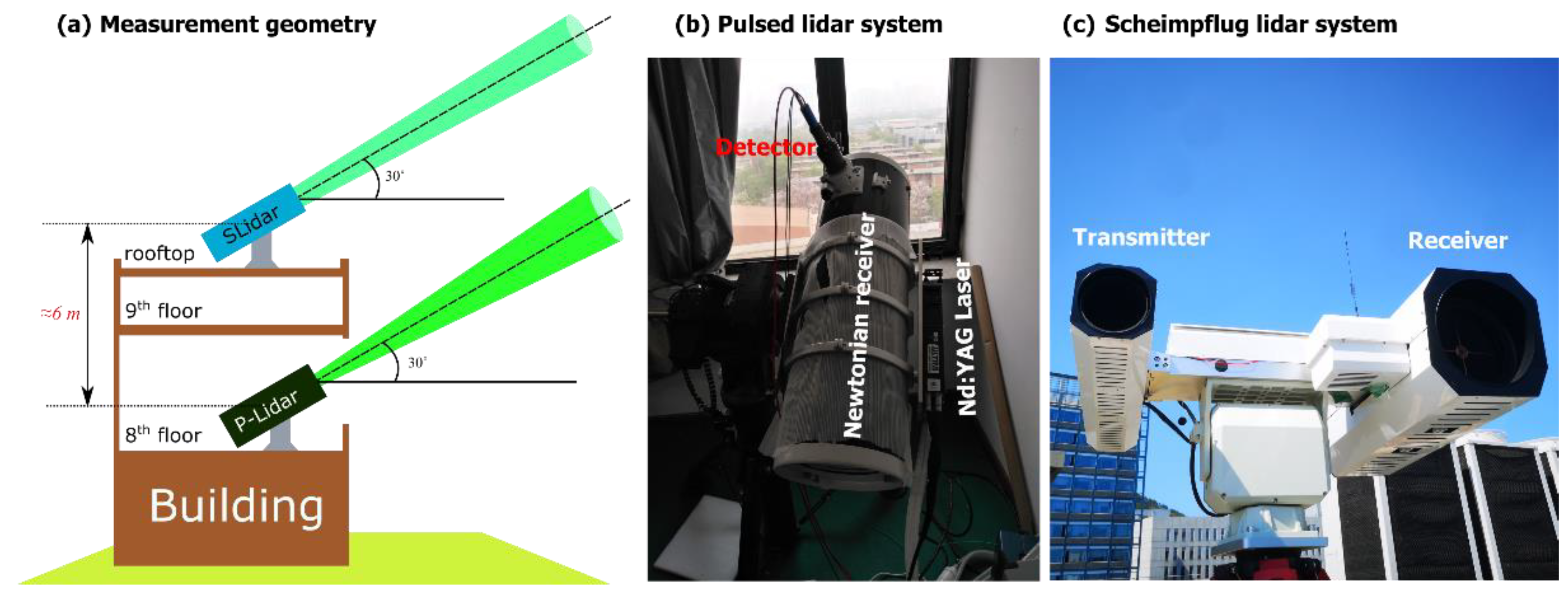
2. Materials and Methods

2.1. The Pulsed lidar System

The principle of the conventional pulsed lidar system has been thoroughly discussed in previous literature [51,52]; only a short introduction of the 532-nm off-axis Mie-scattering pulsed lidar system is given in this work. The pulsed lidar system utilized the second-harmonic (532 nm, 50 mJ/pulse, 20 Hz) of a Nd:YAG laser as the light source. Atmospheric backscattering light was collected by a Newtonian telescope (f = 1000 mm, ∅250 mm) and then collimated by an aspheric lens. The sunlight was suppressed by an interference filter (532 nm) with a 10 nm full-width at half-maximum (FWHM). The lidar signal was detected by a mini photomultiplier tube (PMT, R9880U-110) and acquired by a digitizer (Licel, 20 MHz sampling rate). The lidar data was transferred to a personal computer for data processing. The pulsed lidar system was carried out by an equatorial mount, allowing precise adjustment of the lidar system, as shown in Figure 1b.

2.2. The Scheimpflug Lidar System

The SLidar technique measures the atmospheric backscattering signal with an image sensor placed in a Scheimpflug configuration, namely the image plane, the object plane (laser beam), and the lens plane of the receiving telescope intersect. The SLidar system employed a multi-mode 520-nm laser diode (1 W) as the light source, and a 45° tilted complementary metal-oxide-semiconductor (CMOS) sensor (Lt225NIR, 2048 × 1024 pixels, 5.5 μm) as the detector. The laser beam emitted from the 520-nm laser diode was collimated by a refractor (f = 600 mm, ∅100 mm). The backscattering light was focused on the CMOS sensor by a 200-mm Newtonian telescope (f = 800 mm). A 520-nm interference filter (10-nm FWHM) was mounted in front of the CMOS camera to suppress the sunlight. The separation between the laser beam and the receiver was about 806 nm, ensured by mechanical design, in order to satisfy the Scheimpflug principle. The SLidar system was mounted on a rotation stage (Wanteng, VT-H50) with a maximum elevation angle of 45 degree, as shown in Figure 1c. The laser diode was on-off modulated, and the modulation was synchronized with the exposure of the CMOS sensor. The modulation frequency could change between 1 Hz and 25 Hz depending on the sunlight background intensity. The backscattering image of the laser beam propagating in the atmosphere and the background image with the laser diode turned off can then be alternately recorded, from which the raw lidar signal and the background signal can be retrieved, respectively. The final lidar curve was obtained after background subtraction, signal averaging, digital filtering with the Savitzky-Golay filter, and pixel-distance calibration by measuring the backscattering echo from the wall of a distant tall building (2.3 km away in this work) [53].

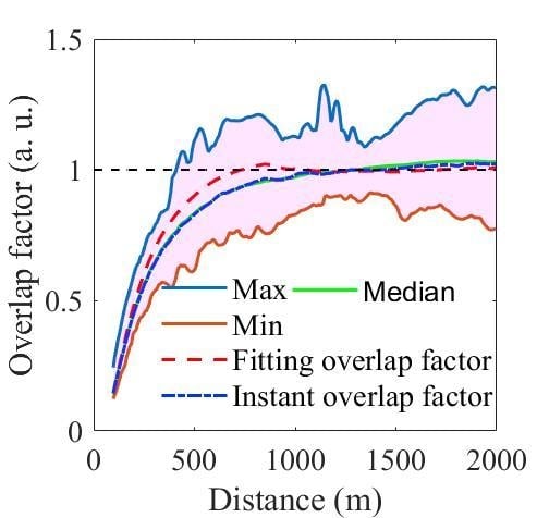
2.3. Calibration Method of the Overlap Factor

The pulsed lidar system has a constant range resolution that is independent of the measurement distance, e.g., 7.5 m (20 MHz sampling rate) or 15 m (10 MHz sampling rate), determined by the sampling rate and the pulse width of the transmitted laser beam. On the other hand, the SLidar technique has a sub-meter range resolution in the near range. However, the range resolution will continuously increase with the increasing of the measurement distance, e.g., 1.5 m at 500 m, 6 m at 1.0 km, and 14 m at 1.5 km. In the region of 2–3 km, the range resolution gets even worse, e.g., 55 m at 3.0 km. Small atmospheric variations may not be visible from the lidar curves measured by the SLidar technique. Thus, the calibration of the overlap factor for the pulsed lidar system should be carried out below 1.5 km, where the range resolution of about 15 m is comparable to most pulsed lidar systems. As the pulsed lidar system and the SLidar system have the same elevation and azimuth angles, the lidar signals recorded by the two-lidar systems should be identical. Direct comparison between the lidar curves measured by the two systems is the most straightforward approach to obtain the overlap factor. According to above discussion, the lidar signals measured by the pulsed lidar system and the SLidar system should satisfy the following relationship:

$$z^2{P}_{\mathrm{p}}(z)=KO(z)P_{\mathrm{s}}(z)$$

(1)

Here, z is the measurement distance, $O(z)$ is the overlap factor of the pulsed lidar system, K is the system constant independent of the measurement distance, $P_{\mathrm{s}}(z)$ is the SLidar signal, and $P_{\mathrm{p}}(z)$ is the pulsed lidar signal. According to the principle of imaging lidar techniques, the lidar signal measured by the SLidar technique is independent of the distance-square factor ($z^2$). Thus, range-correction is not required for the SLidar technique [42]. In the region where the overlap factor of the pulsed lidar system equal to 1, Equation (1) can be simplified as

$$\ln \left[z^2{P}_{\mathrm{p}}(z)\right]=\ln \left[K\right]+\ln \left[P_{\mathrm{s}}(z)\right]$$

(2)

In the region where the pulsed lidar system and the SLidar system have similar performance, e.g., similar range resolution and the same overlap factor of 1 (O(z) = 1), the system constant can be readily obtained by

$$\ln \left[K\right]=mean\left(\ln \left[z^2{P}_{\mathrm{p}}(z)\right]-\ln \left[P_{\mathrm{s}}(z)\right]\right)$$

(3)

Here, “mean” denotes the arithmetic average. Thus, the overlap factor of the pulsed lidar system in the near range can be evaluated with a known system constant according to Equation (1).

3. Results

Experimental measurements have been performed by employing the pulsed lidar system and the SLidar system simultaneously, in Dalian, Northern China. The pulsed lidar system was placed inside a laboratory on the 8th floor of the Graduate Education (GE) building (27 m above the ground), while the SLidar system was located on the roof of the GE building (33 m above the ground). The pulsed lidar system and the SLidar system were pointed to the same direction with an elevation angle of 30˚ for slant atmospheric measurements, limited by the window of the laboratory.

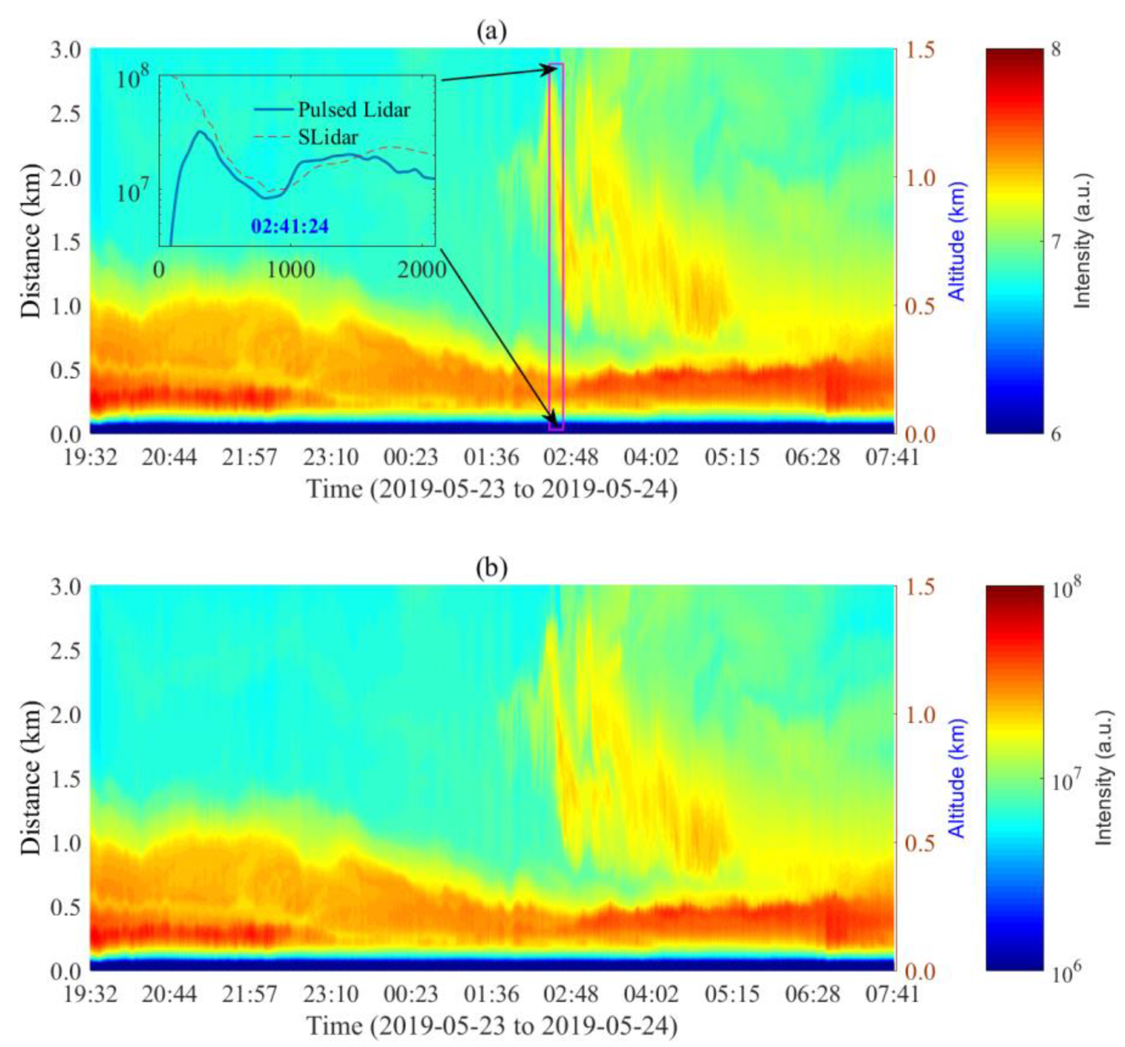
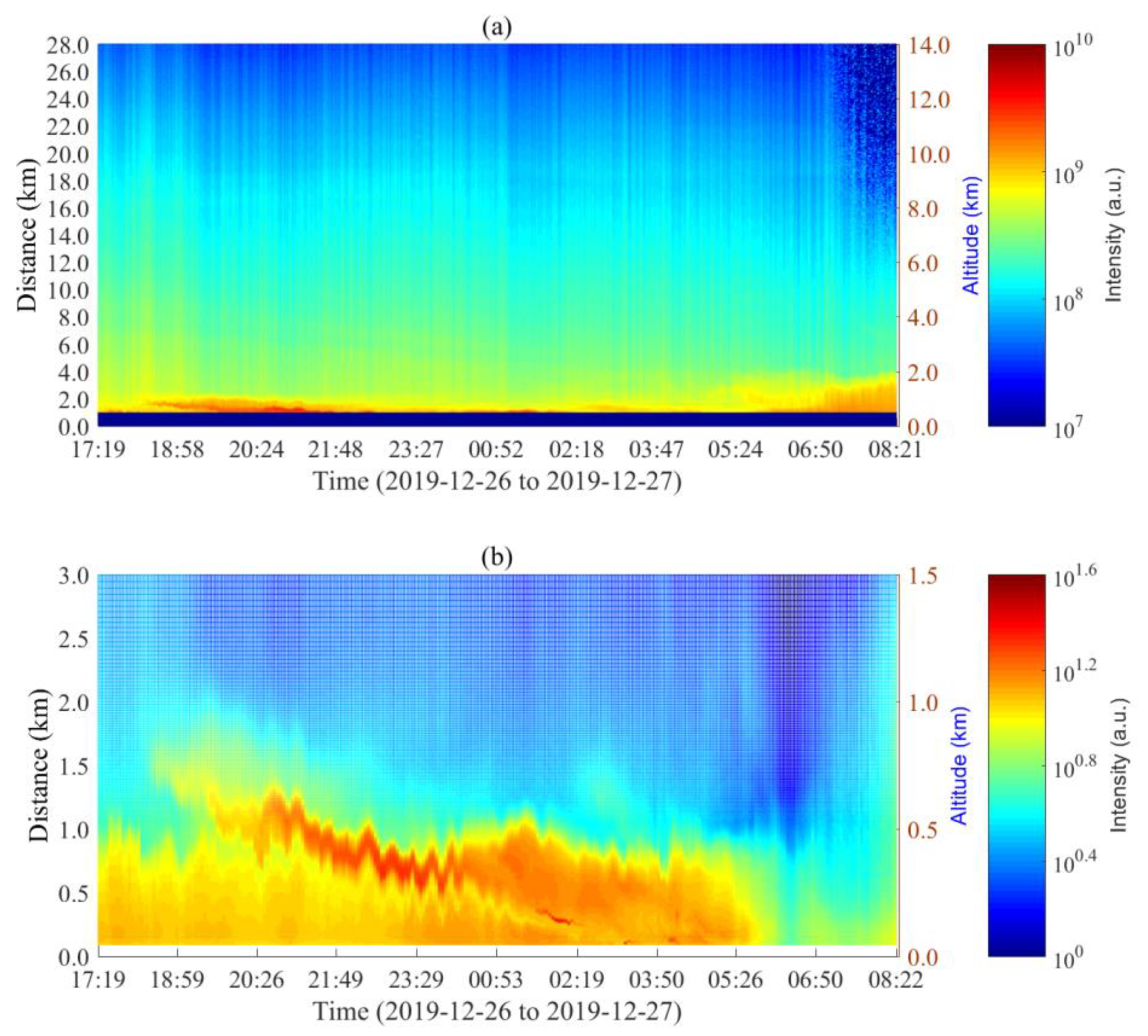
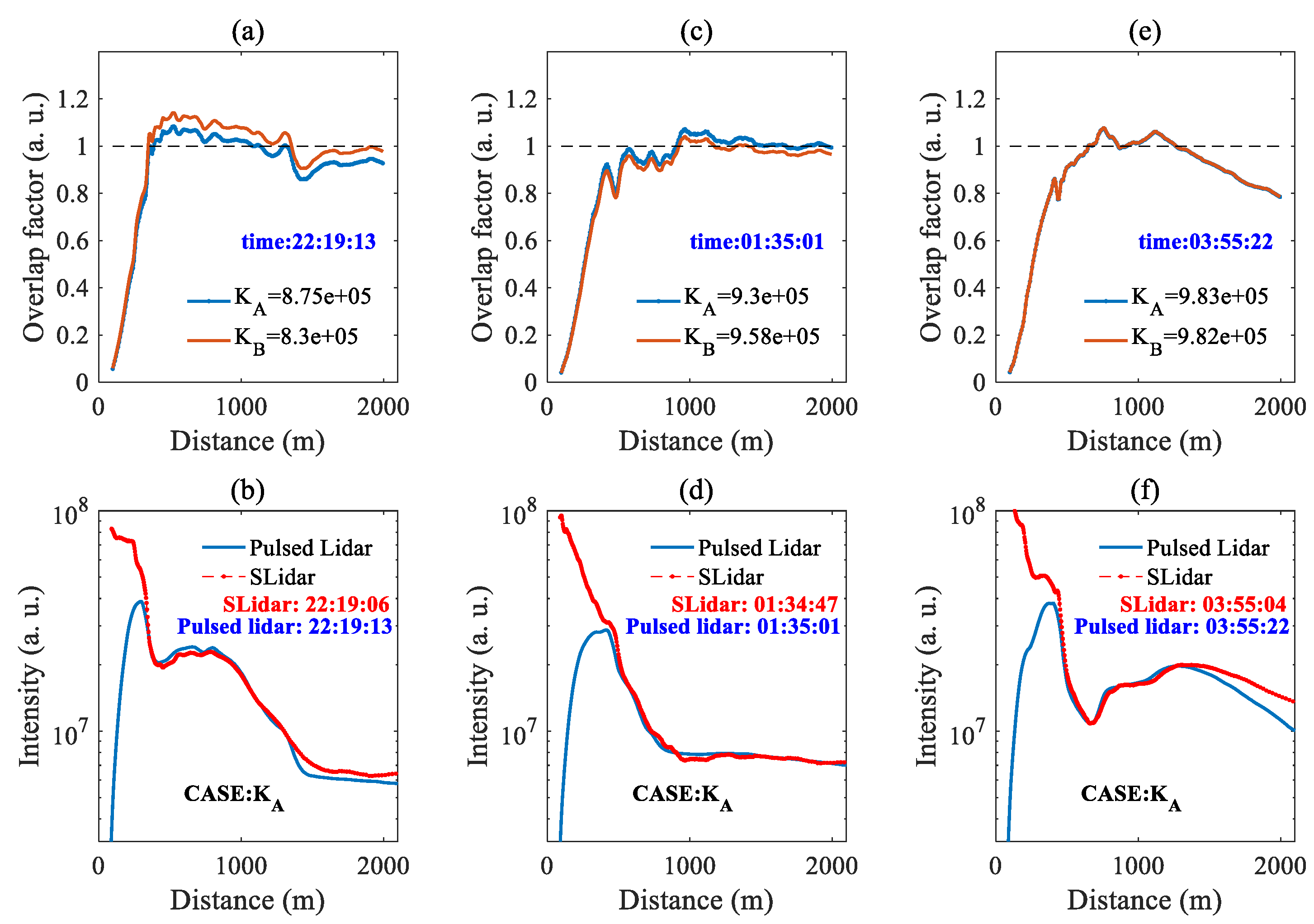
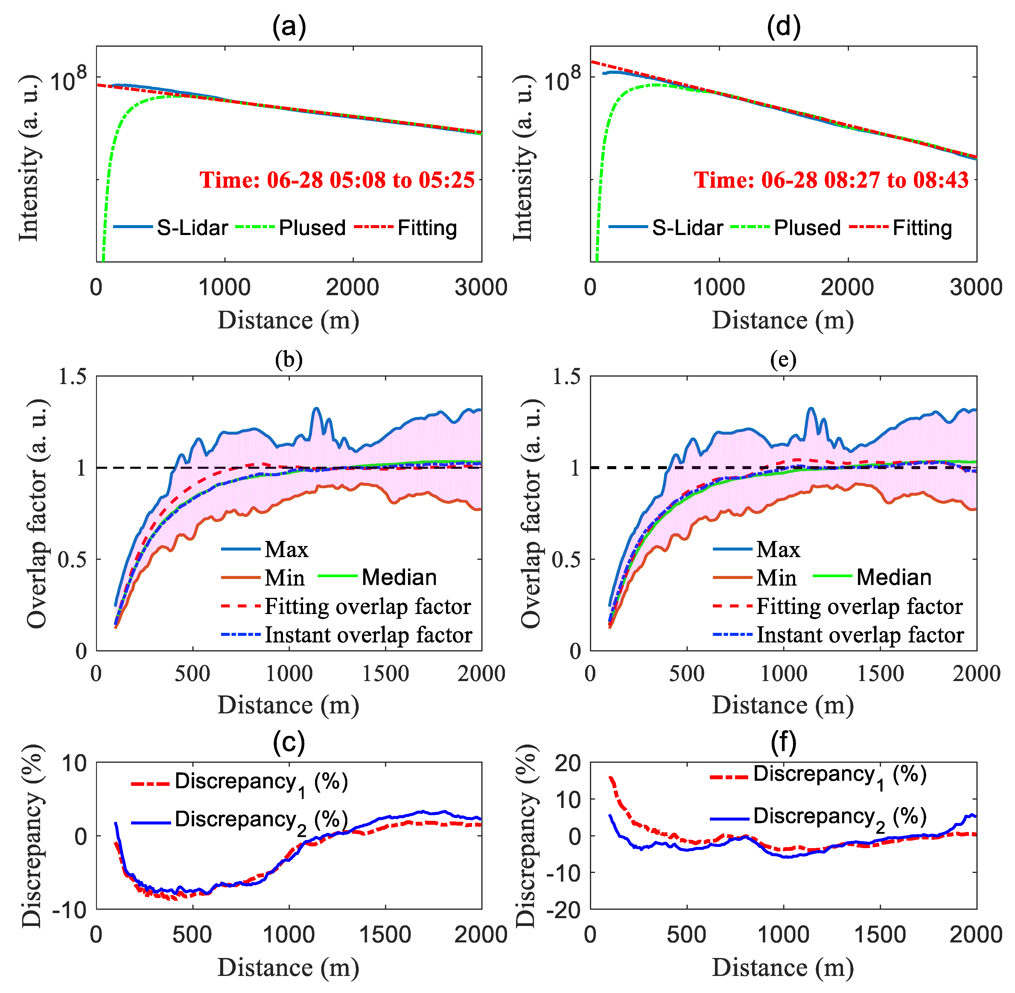
3.1. Atmospheric Slant Measurements for the Overlap Factor Calibration

Slant atmospheric measurements have been performed in May 2019. The elevation angle of the two lidar systems were 30 degrees. The lidar signals have been averaged about 50 s for both lidar systems. The time-spatial maps of the backscattering intensity measured by the SLidar system and the pulsed lidar system are shown in Figure 2a,b, respectively, which are rather similar to each other within 3 km range. As can be seen, the near range lidar curve measured by the pulsed lidar system was poor. Although the pulsed lidar system has been optimized for the detection of the near range lidar signal, the blind range of the pulsed lidar system was still very large, i.e., about 500 m, due to incomplete overlap, etc. Moreover, the near range lidar signals cannot be well resolved due to geometrical compression, etc. Under this circumstance, the overlap factor below 500 m can be calibrated by employing the lidar curves measured by the SLidar system, which will be discussed in detail in the following sections.

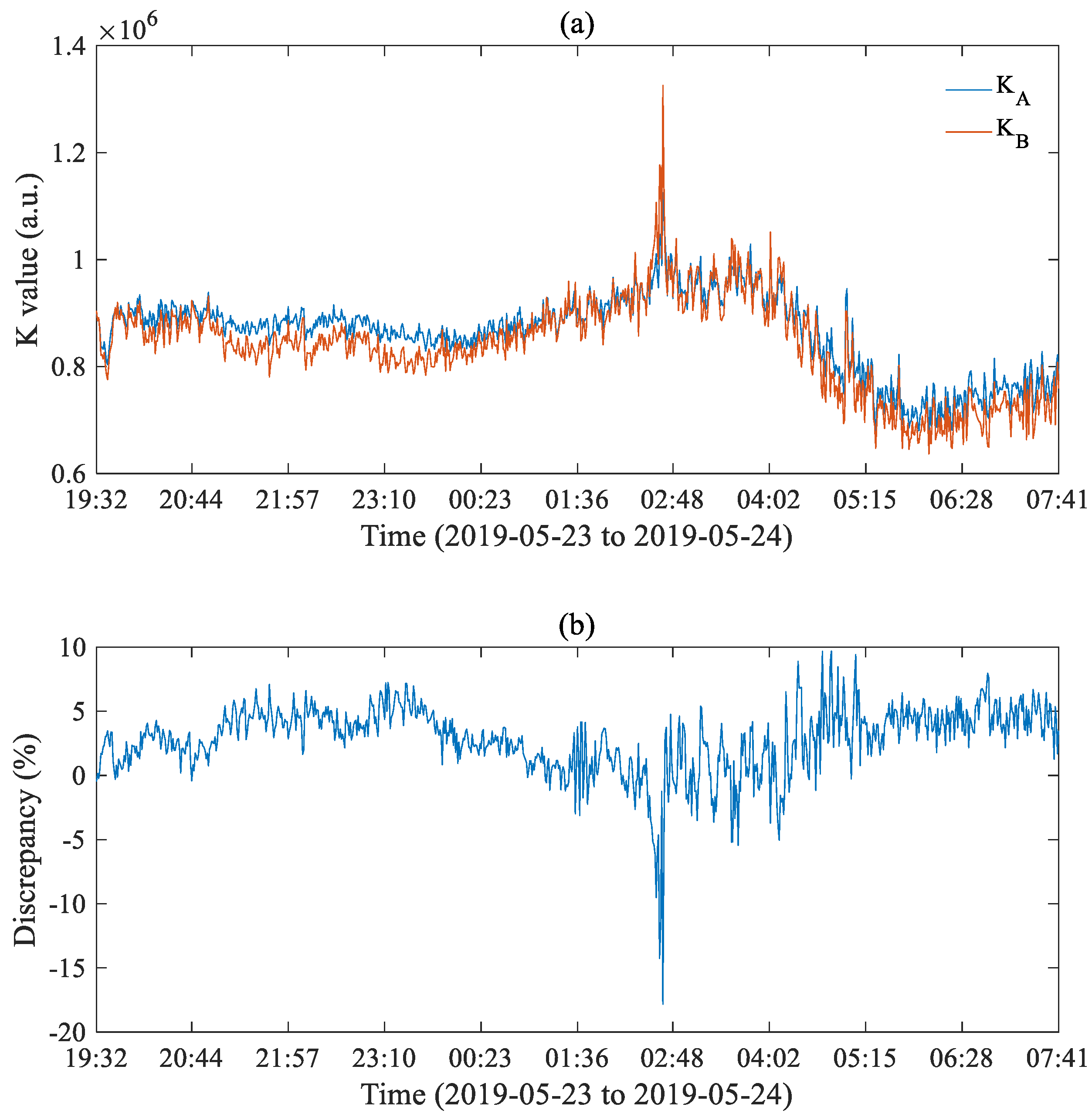
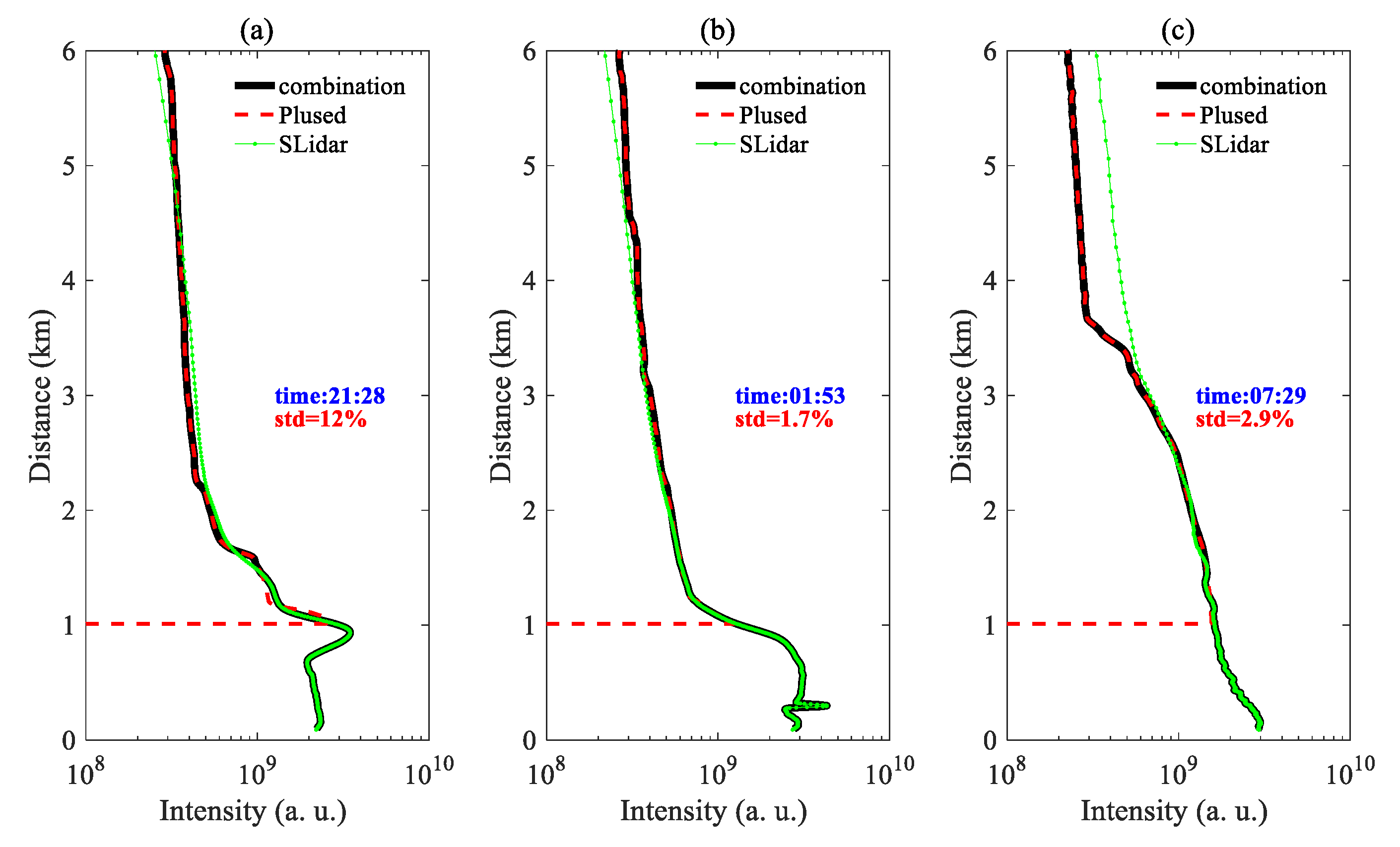
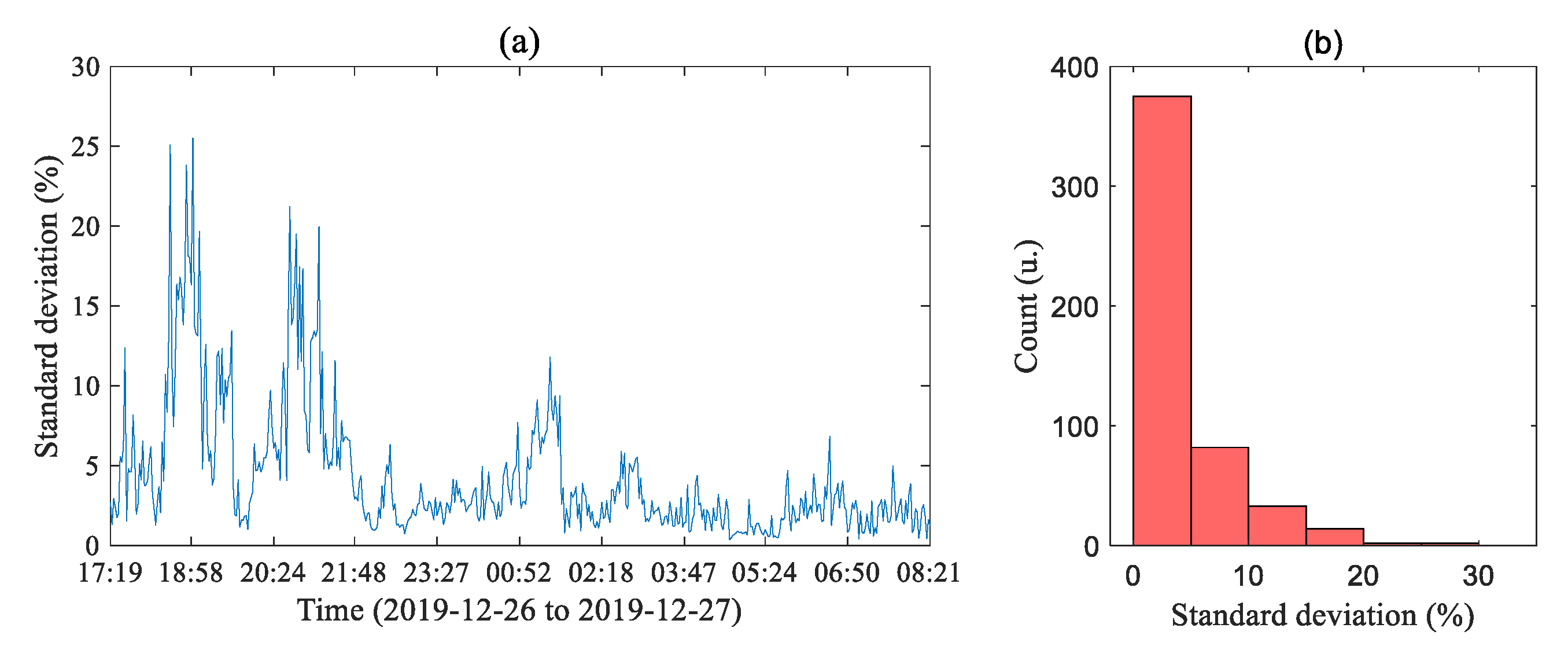
3.2. Horizontal Atmospheric Measurements under Homogeneous Atmospheric Conditions

As has been discussed earlier, the overlap factor may be calibrated by assuming a statistically homogeneous atmospheric condition in the boundary layer. Although the calibration procedure is not difficult and no additional instruments are required, the assumption of homogeneous atmospheric condition was often suspicious for vertical atmospheric measurements. Nevertheless, the atmosphere could be homogeneous in a relatively short region, e.g., several hundred meters (or a few kilometers), on a near horizontal measurement path. Under this circumstance, the overlap factor could be readily calibrated through linear fitting on the log-scale lidar curve measured by the pulsed lidar system, which can be utilized for validating the overlap factor obtained from the SLidar system. Thus, near-horizontal atmospheric measurements have also been performed in June 2019 with the pulsed lidar system and the SLidar system. Each lidar curve has been averaged for about 50 s. During horizontal measurements, the alignment of the pulsed lidar system has changed compared to the measurement performed in slant direction, leading to a larger blind range of around 1000 m. The maps of the backscattering intensities measured by the two systems are shown in Figure 3. Although atmospheric backscattering signal may be observed in 1000 m in Figure 3b, the overlap factor was less than one in this region, as will be discussed later.

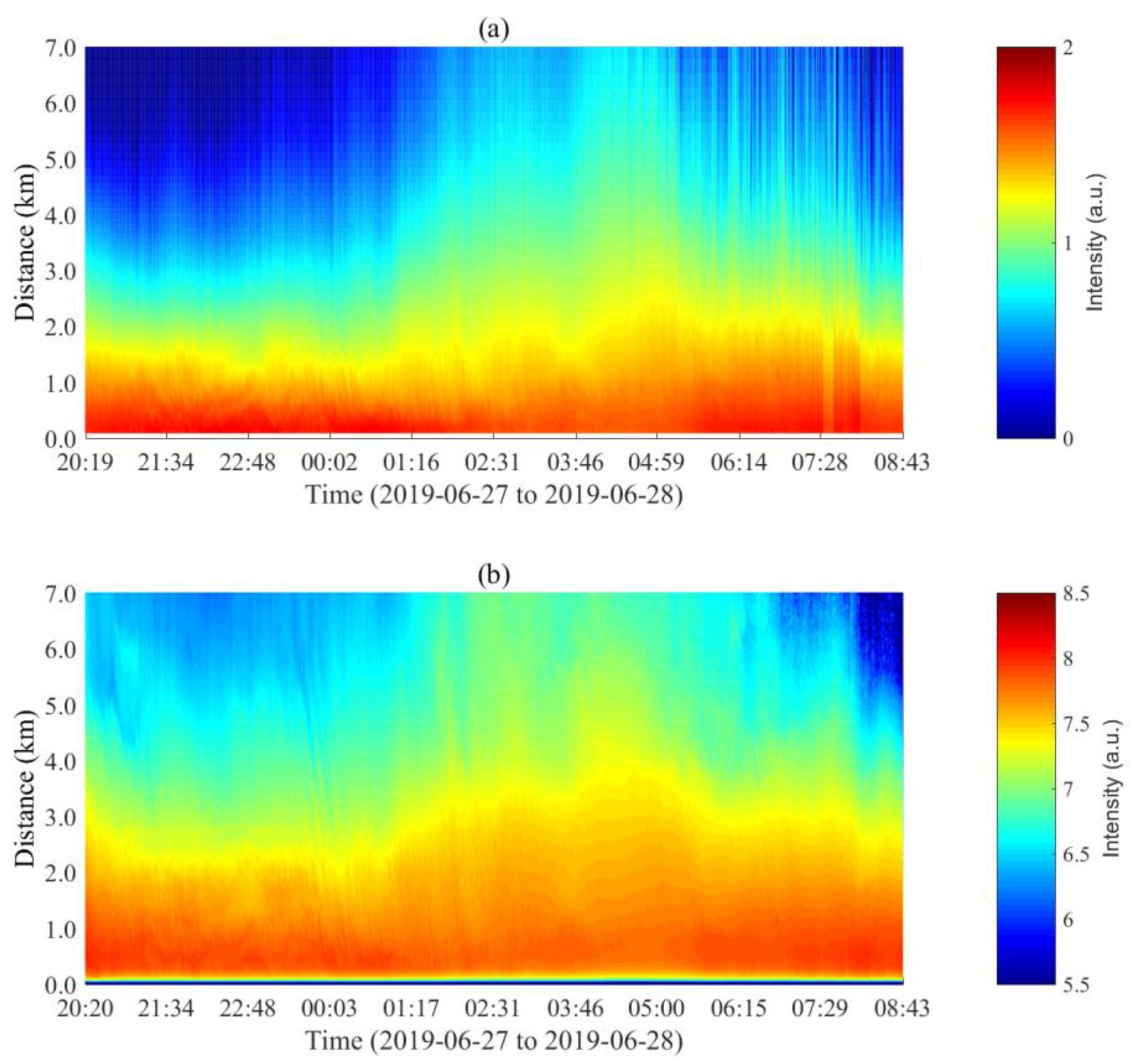
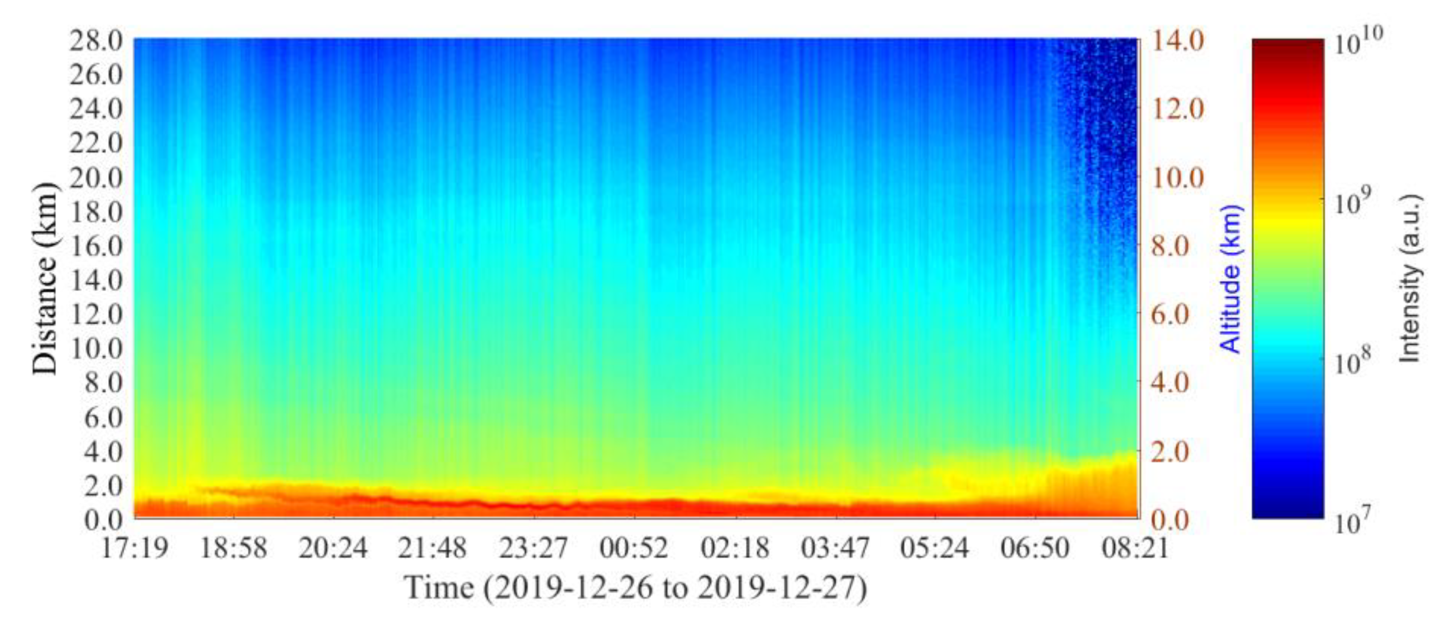
3.3. Far-Range Atmospheric Measurements

The conventional pulsed lidar technique can measure atmospheric aerosol structure up to tens of kilometers by employing high-power pulsed lasers and large receiving aperture with a diameter in the order of meter. When the system performance is optimized for far range detection, the lidar signal in the near range is either unavailable or has a very low quality due to geometrical compressions, insufficient size of the PMT detect, signal saturation and PMT gating time, etc. Nevertheless, the SLidar technique has a sub-meter range resolution in the near range and a short blind range less than 100 m without any calibrations. Thus, a combination measurement employing the pulsed lidar and the SLidar cannot only achieve a far detection range but also a short blind range.

In this work, a combination measurement campaign, employing collocated pulsed lidar system and SLidar system, has been carried out in December 2019 to extend the measurement range of the pulsed lidar system. The performance of the pulsed lidar system was optimized for long distance measurement. The PMT voltage was gated on at around 1 km distance. The pulsed lidar system can then measure the atmospheric backscattering signal up to 28 km during nighttime and 11 km during daytime, with a signal averaging time of 100 s and a threshold signal-to-noise ratio (SNR) of 10. As shown in Figure 4a, the blind range of the pulsed lidar measurements was about 1 km, while the SLidar system can measure near ground atmospheric structures up to 90 m, where atmospheric turbulence can be clearly observed between 500–1000 m (250–500 m in altitude). A measurement range covering from the near ground at around 90 m up to 28 km can then be achieved by gluing the lidar curves measured by the two systems.

4. Discussion

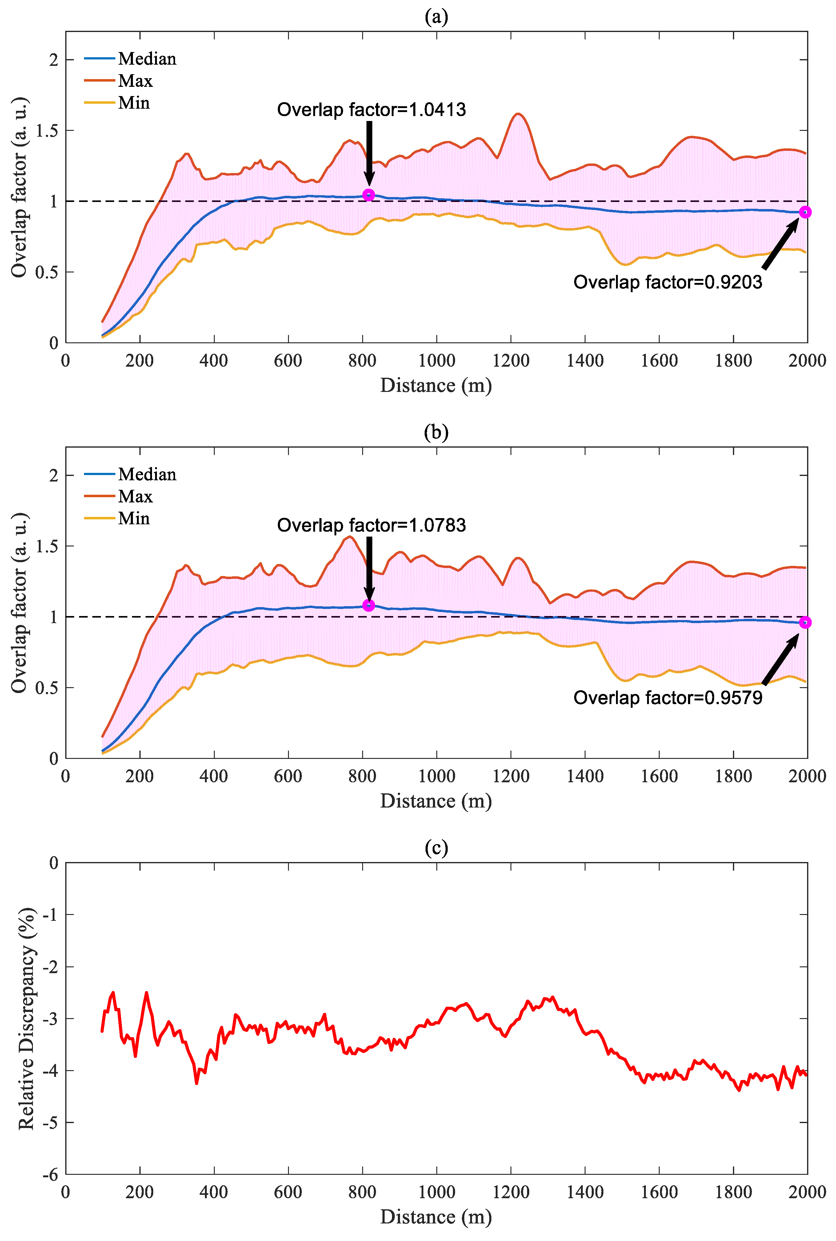
4.1. Studies on the Overlap Factor

According to above discussion, the system constant K should be pre-determined before the retrieval of the overlap factor. Owing to the varying range resolution, the SLidar technique can detect small spatial variation in the near range (particularly below 500 m), and it could also smooth the lidar curves around and beyond 2 km. In order to evaluate the performance of employing lidar curves in different measurement regions for the overlap factor calibration, the system constant has been estimated in two regions, namely the region A and the region B. The region A was defined as 500–1500 m, considering a blind range of 500 m of the pulsed lidar system and the range resolution of the SLidar system. The region B was defined as 1050–1500 m, where the range resolution of the SLidar system (6 m at 1000 m, and 14 m at 1500 m) was slightly worse but still comparable to that of the present pulsed lidar system. The corresponding system constants were denoted as K_A and K_B, respectively. Since the lidar curves were recorded by different computers, the evaluation of the system constant was performed for lidar curves with closest recording times. Meanwhile, the lidar curves measured by the SLidar system have been interpolated with an equal range interval of 7.5 m for comparison studies.

As can be seen in Figure 5a, the system constant has shown a clear temporal variation, indicating substantial drifting of the system parameters, e.g., the emitted laser power. However, the values of K_A and K_B were still rather close to each other. The relative discrepancy between K_A and K_B, namely (K_A − K_B)/K_A, was generally less than 10% as shown in Figure 5b, apart from the lidar curves measured at around 02:30. The suddenly increased system constant as well as the discrepancy could be due to the appearing of the aerosol load beyond 1 km, resulting in substantial heterogeneity of the aerosol distribution in the measurement volume, as can be seen from the inset of Figure 2a.

Overlap factors were evaluated in different atmospheric conditions according to Equation (1) using the system constants obtained in the two regions, as shown in Figure 6. The system constants calibrated in the region of 500–1500 m and 1050–1500 m were referred to as K_A and K_B, respectively. The lidar signal measured by the SLidar system has been multiplied by the system constant K_A. As can be seen, the overlap factor has also shown clear temporal variations. Moreover, the overlap factor in the region of 500–2000 m did not equal to 1; it instead fluctuated around 1. The fluctuation may reach up to 20% around 2000 m, as shown in Figure 6e. This indicated that the atmospheric backscattering signals measured by the pulsed lidar system and the SLidar system were not fully identical. A main reason for the discrepancies between the lidar curves was that the pulsed lidar system and the SLidar system did not exactly measure the same volume, in spite that they were very close to each other (6 m away in horizontal direction). The atmospheric heterogeneity can introduce large discrepancies on the lidar curves, as shown in Figure 6e,f. On the other hand, the difference in range resolution between the SLidar technique and the pulsed lidar technique could also influence the calibration of the overlap factor, particularly in the near range. As can be seen in Figure 6e, a small dip was observed in the overlap factor. Moreover, Simeonov et al. have shown that the spatial uniformity of the PMT could have significant influence on the lidar signal particularly for the near range lidar curves [54].

Statistical analysis on the overlap factor has been performed by investigating the overlap factor retrieved during the whole measurement period. The statistical maximum, minimum and median values of the overlap factor, evaluated from lidar curves recorded during the whole measurement period, are shown in Figure 7a,b. It can be found out that the overlap factor was less than one for a measurement distance less than 500 m. The maximum and the minimum boundary of the overlap factor indicated the fluctuations of the lidar signals measured by the two systems, due to atmospheric heterogeneity, and varying range resolution of the SLidar technique, etc. Nevertheless, the influence of the atmospheric heterogeneity can be mitigated in the median value of the overlap factor. In the region between 500–2000 m, the deviation of the median overlap factor to one was between −8% and 4% for the system constant calibrated in the region A, while it varied between −4% and 8% for the system constant calibrated in the region B. The relative discrepancy between the median overlap factors was also less than 5%, as shown in Figure 7c, implying a promising result of employing both regions A and B for the calibration of the system constant and thus the overlap factor.

Joint measurements using the pulsed lidar system and the SLidar system have been carried out on a near-horizontal measurement geometry. Figure 8a,d shows lidar curves recorded in the morning at around 05:00 and 08:30 on 28th June 2019, respectively, which were statistical median values of 20 lidar curves recorded in about 17 min (50 s for each lidar curve). As can be seen, the lidar curves measured by both systems were nearly straight lines in the region of 1–3.0 km, implying a relatively homogeneous atmospheric condition. A linear fitting on the log-scale pulsed lidar curve in the region of 1–3.0 km has been performed. As can be seen from Figure 8a,d, the lidar curve measured by the SLidar system generally agreed with the linear fitting in the region of 0.1–1.0 km. Thus, the overlap factor of the pulsed lidar system is obtained by dividing the pulsed lidar curve with the corresponding fitting curve (dashed curve), referred to as the fitting overlap factor. According to Equations (1)–(3), the instant overlap factor could also be obtained by dividing the lidar curve measured by the pulsed lidar system with the lidar curve measured by the SLidar system with the system constant calibrated in the region of 1.05–1.5 km. The statistical values of the overlap factor have also been evaluated from the experimental curves recorded during the whole measurement period (from 27 June to 28 June).

As shown in Figure 8b,d, the overlap factors evaluated from different approaches agreed quite well, in spite that the maximum and the minimum value of the overlap factor varied quite a lot due to atmospheric heterogeneity. The discrepancy between the median overlap factor (the instant overlap factor) and the fitting overlap factor was generally less than 10% for most measurement ranges. The relatively larger discrepancy between the instance overlap factor and the fitting overlap factor in the near region could be mainly due to the fact that spatial variation still existed, where the SLidar technique had very high range resolution. Moreover, statistical analysis on horizontal comparison measurements performed from 20:30 on 25 June to 08:49 on 26 June has also revealed that the median overlap factor and the fitting overlap factor were also in good agreement, with the discrepancy generally less than 10%. This promising result successfully demonstrated a great potential of employing the far range (1050–1500 m) lidar signal for the calibration of the system constant and the overlap factor, which was particularly useful when the lidar signal below 1000 m was poor or unavailable.

4.2. Atmospheric Remote Sensing with a Large Measurement Range

As has been discussed in Section 4.1, the system constant can also be calibrated in the region between 1.0 and 1.5 km by comparing lidar curves measured by the SLidar system and the pulsed lidar system. A lidar curve, consisting of the lidar signal measured by the SLidar system in the region below 1.05 km and the lidar signal measured by the pulsed lidar system beyond 1.05 km, can be obtained by gluing the lidar curves in the region of 1.05–1.5 km. The standard deviation between the lidar curves in the gluing region (1.05–1.5 km) was calculated by

$$std=\frac{{\displaystyle {\sum }_{1050}^{1500}{\left[\left(z^2{P}_{\mathrm{p}}(z)-K{P}_{\mathrm{s}}(z)\right)/\left(z^2{P}_{\mathrm{p}}(z)\right)\right]}^2}}{N-1}\times 100\%$$

(4)

Figure 9 shows the glued lidar curves and the corresponding standard deviations under different atmospheric conditions. The standard deviation generally increased, when large atmospheric variation in vertical direction appeared. Statistical analysis on the standard deviation has also been performed. As shown in Figure 10a, the standard deviation was generally less than 25%, with a mean value of 4%. The relatively larger standard deviation mainly occurred for the lidar curves with large spatial variations. The lidar curves measured during the early morning also had a rather small standard deviation, although the SNR deteriorated due to the increasing of the sunlight background. In summary, most glued lidar curves (90% of the measurements) had a standard deviation less than 10%, as indicated by Figure 10b. The temporal and spatial distribution of the glued atmospheric backscattering signal, covering the range from 90 m to 28 km, is shown in Figure 11.

The aerosol extinction coefficient can then be obtained according to the Fernald algorithm with the lidar ratio empirically determined to be 50 sr [55,56,57]. For nighttime measurements, the boundary value of the aerosol extinction coefficient was estimated in the clean layer, i.e., 28 km in this study (14 km in altitude), where the aerosol load was assumed negligible. During daytime measurements (early morning), the SNR of the far-range lidar signal deteriorated, the measurement range was limited to about 11 km (5.5 km in altitude). The clean layer assumption was not reliable in this case. Thus, the boundary value of the aerosol extinction coefficient was then estimated according to the slope method by finding a homogeneous region in the region below 11 km with the Douglas-Peucker algorithm [58]. The ambient temperature and the relative humidity were recorded by an air-pollution monitor (FairSense A108). The temperature profile was evaluated according to the model of the U.S. Standard Atmosphere. The map of the retrieved aerosol extinction coefficient is shown in Figure 12. As can be seen, the aerosol load was mainly concentrated in the low altitude below 2 km (4 km in distance). The near-ground atmospheric aerosol variation can also be well resolved from the extinction profile, as shown in Figure 12b. Beyond 4 km (2 km in altitude), the aerosol extinction coefficient was generally less than 0.03 km⁻¹.

In order to validate the measurement result, the aerosol extinction coefficient retrieved in the near ground (below 200 m distance, 100 m in altitude) was evaluated for comparison studies with the PM10 concentration measured by a pollution monitoring station located at 2.5 km away from the lidar system (Qixianling Station). As shown in Figure 13, the median aerosol extinction coefficients at different altitudes have shown similar temporal variations with the PM10 concentration from 17:00 on 26th December to about 07:00 On 27th December. In the early morning on 27th December (07:00–08:00), the aerosol extinction coefficient quickly decreased possibly due to the growth of the boundary layer driven by sunlight heating, in spite that the relative humidity also increased. However, the PM10 concentration was continuously increasing. Moreover, the PM10 concentrations reported by other pollution monitoring stations, which were several kilometers away from the lidar systems, also increased continuously. The inverse relationship between the aerosol extinction coefficient in 50–100 m altitude and the near ground PM10 concentration implied that the PM10 concentration also had a large spatial variation even in the near surface. On the other hand, the PM10 concentration measured by the Qixianling national station started to decrease after 09:00 on 27 December. This phenomenon further confirmed that the monitoring of the near ground aerosol distribution was of great significance for understanding atmospheric chemistry and environmental monitoring. SLidar systems with even shorter blind range (e.g., 30 m or even 10 m) and all-day measurement capability were highly demanded for future atmospheric aerosol monitoring applications.

5. Conclusions

As a powerful active remote sensing tool, lidar is capable of measuring atmospheric aerosol profile up to tens of kilometers. Nevertheless, the prevailing pulsed lidar techniques face a significant challenge in the retrieval of the near surface aerosol profile, which is of great importance for meteorological applications and environmental monitoring. In this work, the SLidar technique, featuring of short blind range, low cost and low maintenance, has been employed to overcome the challenge of the conventional pulsed lidar technique. The overlap factor of the pulsed lidar system can be experimentally calibrated by using a collocated SLidar system. The system constant, retrieved by comparing lidar curves in the region of 500–1500 m (region A) and 1050–1500 m (region B), was in good agreement with each other and has been successfully utilized for the retrieval of the overlap factor. The calibrated median overlap factor in the region of 500–2000 m varied between −8%–4% for the system constant calibrated in the region A and −4%–8% for the system constant calibrated in the region B. Horizontal comparison measurements have also been conducted to validate the reliability of the retrieved overlap factor. It has been found out that the median overlap factor evaluated by the presented method agreed very well with the overlap factor obtained by the linear fitting approach with the assumption of homogeneous atmospheric condition, with a discrepancy less than 10%. The promising result has shown a great potential of employing a collocated SLidar system to calibrate the overlap factor of the conventional pulsed lidar system. Moreover, SLidar systems operating at 375 nm, and 1064 nm, etc., can also be implemented for calibrating the overlap factor of the pulsed lidar system operating at various wavelengths.

Motivated by the promising result, a joint measurement campaign has been carried out by employing the pulsed lidar system and the SLidar system. A measurement range of up to 28 km (SNR ≥ 10) has been achieved during the nighttime by gluing the lidar signals measured by the two systems. The maximum measurement range during daytime (11 km) can be greatly improved by changing the broadband filter (10 nm) into a narrow band interference filter, e.g., 0.5 nm, which has been widely utilized in conventional pulsed lidar systems. The aerosol extinction profile in the near surface beyond 90 m can be well resolved owing to the sub-meter range resolution of the SLidar technique. The aerosol extinction coefficient in the low altitude (50–100 m) was generally in good agreement with the PM10 concentration measured by a pollution monitoring station. Nevertheless, an inverse relationship between the aerosol extinction coefficient in 50–100 m altitude and the near ground PM10 concentration has also been observed in the early morning after sunrise. This phenomenon further demonstrated that SLidar systems with even shorter blind range (e.g., 30 m or even 10 m) and all-day measurement capability were highly demanded for future atmospheric applications. The blind range of the SLidar system could be reduced by employing a receiver with a shorter focal length or an image sensor with a larger area. The daytime performance of the SLidar technique can be further enhanced for all-day measurements by improving the geometrical coupling efficiency of the 520-nm laser beam through the collimation lens [59], as well as using narrowband filters or CMOS cameras with larger quantum efficiencies, etc.

References

1. Mamouri, R.E.; Papayannis, A.; Amiridis, V.; Muller, D.; Kokkalis, P.; Rapsomanikis, S.; Karageorgos, E.T.; Tsaknakis, G.; Nenes, A.; Kazadzis, S.; et al. Multi-wavelength Raman lidar, sun photometric and aircraft measurements in combination with inversion models for the estimation of the aerosol optical and physico-chemical properties over Athens, Greece. Atmos. Meas. Tech. 2012, 5, 1793–1808. [Google Scholar] [CrossRef]
2. Marchant, C.C.; Wilkerson, T.D.; Bingham, G.E.; Zavyalov, V.V.; Andersen, J.M.; Wright, C.B.; Cornelsen, S.S.; Martin, R.S.; Silva, P.J.; Hatfield, J.L. Aglite lidar: A portable elastic lidar system for investigating aerosol and wind motions at or around agricultural production facilities. J. Appl. Remote Sens. 2009, 3, 033511. [Google Scholar] [CrossRef]
3. Pappalardo, G.; Amodeo, A.; Apituley, A.; Comeron, A.; Freudenthaler, V.; Linne, H.; Ansmann, A.; Bosenberg, J.; D’Amico, G.; Mattis, I.; et al. EARLINET: Towards an advanced sustainable European aerosol lidar network. Atmos. Meas. Tech. 2014, 7, 2389–2409. [Google Scholar] [CrossRef] [Green Version]
4. Kulla, B.S.; Ritter, C. Water vapor calibration: Using a Raman lidar and radiosoundings to obtain highly resolved water vapor profiles. Remote Sens. 2019, 11, 616. [Google Scholar] [CrossRef] [Green Version]
5. Shiina, T. LED mini lidar for atmospheric application. Sensors 2019, 19, 569. [Google Scholar] [CrossRef] [PubMed] [Green Version]
6. Banakh, V.A.; Smalikho, I.N. Lidar studies of wind turbulence in the stable atmospheric boundary layer. Remote Sens. 2018, 10, 1219. [Google Scholar] [CrossRef] [Green Version]
7. Hildebrand, J.; Baumgarten, G.; Fiedler, J.; Lubken, F.J. Winds and temperatures of the Arctic middle atmosphere during January measured by Doppler lidar. Atmos. Chem. Phys. 2017, 17, 13345–13359. [Google Scholar] [CrossRef] [Green Version]
8. Caicedo, V.; Rappengluck, B.; Lefer, B.; Morris, G.; Toledo, D.; Delgado, R. Comparison of aerosol lidar retrieval methods for boundary layer height detection using ceilometer aerosol backscatter data. Atmos. Meas. Tech. 2017, 10, 1609–1622. [Google Scholar] [CrossRef] [Green Version]
9. Baars, H.; Seifert, P.; Engelmann, R.; Wandinger, U. Target categorization of aerosol and clouds by continuous multiwavelength-polarization lidar measurements. Atmos. Meas. Tech. 2017, 10, 3175–3201. [Google Scholar] [CrossRef] [Green Version]
10. Parracino, S.; Richetta, M.; Gelfusa, M.; Malizia, A.; Bellecci, C.; De Leo, L.; Perrimezzi, C.; Fin, A.; Forin, M.; Giappicucci, F.; et al. Real-time vehicle emissions monitoring using a compact LiDAR system and conventional instruments: First results of an experimental campaign in a suburban area in southern Italy. Opt. Eng. 2016, 55, 103107. [Google Scholar] [CrossRef]
11. Wang, J.; Zhang, L.; Huang, J.P.; Cao, X.J.; Liu, R.J.; Zhou, B.; Wang, H.B.; Huang, Z.W.; Bi, J.R.; Zhou, T.; et al. Macrophysical and optical properties of mid-latitude cirrus clouds over a semi-arid area observed by micro-pulse lidar. J. Quant. Spectrosc. Rad. Transf. 2013, 122, 3–12. [Google Scholar] [CrossRef]
12. Sakai, T.; Nagai, T.; Izumi, T.; Yoshida, S.; Shoji, Y. Automated compact mobile Raman lidar for water vapor measurement: Instrument description and validation by comparison with radiosonde, GNSS, and high-resolution objective analysis. Atmos. Meas. Tech. 2019, 12, 313–326. [Google Scholar] [CrossRef] [Green Version]
13. Liu, L.P.; Ruan, Z.; Zheng, J.F.; Gao, W.H. Comparing and merging observation data from Ka-band cloud radar, C-Band frequency-modulated continuous wave radar and Ceilometer systems. Remote Sens. 2017, 9, 1282. [Google Scholar] [CrossRef] [Green Version]
14. Papayannis, A.; Chourdakis, G. The EOLE Project: A multiwavelength laser remote sensing (lidar) system for ozone and aerosol measurements in the troposphere and the lower stratosphere. Part II: Aerosol measurements over Athens, Greece. Int. J. Remote Sens. 2002, 23, 179–196. [Google Scholar] [CrossRef]
15. Baars, H.; Kanitz, T.; Engelmann, R.; Althausen, D.; Heese, B.; Komppula, M.; Preissler, J.; Tesche, M.; Ansmann, A.; Wandinger, U.; et al. An overview of the first decade of Polly(NET): An emerging network of automated Raman-polarization lidars for continuous aerosol profiling. Atmos. Chem. Phys. 2016, 16, 5111–5137. [Google Scholar] [CrossRef] [Green Version]
16. Sicard, M.; Molero, F.; Guerrero-Rascado, J.L.; Pedros, R.; Exposito, F.J.; Cordoba-Jabonero, C.; Bolarin, J.M.; Comeron, A.; Rocadenbosch, F.; Pujadas, M.; et al. Aerosol lidar intercomparison in the framework of SPALINET-The Spanish lidar network:methodology and results. IEEE Trans. Geosci. Remote Sens. 2009, 47, 3547–3559. [Google Scholar] [CrossRef] [Green Version]
17. Wandinger, U.; Freudenthaler, V.; Baars, H.; Amodeo, A.; Engelmann, R.; Mattis, I.; Gross, S.; Pappalardo, G.; Giunta, A.; D’Amico, G.; et al. EARLINET instrument intercomparison campaigns: Overview on strategy and results. Atmos. Meas. Tech. 2016, 9, 1001–1023. [Google Scholar] [CrossRef] [Green Version]
18. Adam, M.; Turp, M.; Horseman, A.; Ordonez, C.; Buxmann, J.; Sugier, J. From operational ceilometer network to operational lidar network. EPJ Web Conf. 2016, 119, 27007. [Google Scholar] [CrossRef] [Green Version]
19. Nishizawa, T.; Sugimoto, N.; Matsui, I.; Shimizu, A.; Higurashi, A.; Jin, Y. The Asian dust and aerosol lidar observation network (Ad-Net): Strategy and progress. EPJ Web Conf. 2016, 119, 19001. [Google Scholar] [CrossRef] [Green Version]
20. Halldorsson, T.; Langerholc, J. Geometrical form factors for the lidar function. Appl. Opt. 1978, 17, 240–244. [Google Scholar] [CrossRef]
21. Sassen, K.; Dodd, G.C. Lidar crossover function and misalignment effects. Appl. Opt. 1982, 21, 3162–3165. [Google Scholar] [CrossRef] [PubMed]
22. Ancellet, G.M.; Kavaya, M.J.; Menzies, R.T.; Brothers, A.M. Lidar telescope overlap function and effects of misalignment for unstable resonator transmitter and coherent receiver. Appl. Opt. 1986, 25, 2886. [Google Scholar] [CrossRef]
23. Pal, S. Monitoring depth of shallow atmospheric boundary layer to complement LiDAR measurements affected by partial overlap. Remote Sens. 2014, 6, 8468–8493. [Google Scholar] [CrossRef] [Green Version]
24. Stelmaszczyk, K.; Dell’Aglio, M.; Chudzynski, S.; Stacewicz, T.; Woste, L. Analytical function for lidar geometrical compression form-factor calculations. Appl. Opt. 2005, 44, 1323–1331. [Google Scholar] [CrossRef] [PubMed]
25. Berezhnyy, I. A combined diffraction and geometrical optics approach for lidar overlap function computation. Opt. Laser Eng. 2009, 47, 855–859. [Google Scholar] [CrossRef]
26. Gong, W.; Mao, F.Y.; Li, J. OFLID: Simple method of overlap factor calculation with laser intensity distribution for biaxial lidar. Opt. Commun. 2011, 284, 2966–2971. [Google Scholar] [CrossRef]
27. Kuze, H.; Kinjo, H.; Sakurada, Y.; Takeuchi, N. Field-of-view dependence of lidar signals by use of Newtonian and Cassegrainian telescopes. Appl. Opt. 1998, 37, 3128–3132. [Google Scholar] [CrossRef]
28. Povey, A.C.; Grainger, R.G.; Peters, D.M.; Agnew, J.L.; Rees, D. Estimation of a lidar’s overlap function and its calibration by nonlinear regression. Appl. Opt. 2012, 51, 5130–5143. [Google Scholar] [CrossRef]
29. Mao, F.; Gong, W.; Li, J. Geometrical form factor calculation using Monte Carlo integration for lidar. Opt. Laser Technol. 2012, 44, 907–912. [Google Scholar] [CrossRef]
30. Li, J.; Li, C.C.; Zhao, Y.M.; Li, J.; Chu, Y.Q. Geometrical constraint experimental determination of Raman lidar overlap profile. Appl. Opt. 2016, 55, 4924–4928. [Google Scholar] [CrossRef]
31. Sasano, Y.; Shimizu, H.; Takeuchi, N.; Okuda, M. Geometrical form-factor in the laser-radar equation—Experimental-determination. Appl. Opt. 1979, 18, 3908–3910. [Google Scholar] [CrossRef] [PubMed]
32. Dho, S.W.; Park, Y.J.; Kong, H.J. Experimental determination of a geometric form factor in a lidar equation for an inhomogeneous atmosphere. Appl. Opt. 1997, 36, 6009–6010. [Google Scholar] [CrossRef] [PubMed]
33. Wandinger, U.; Ansmann, A. Experimental determination of the lidar overlap profile with Raman lidar. Appl. Opt. 2002, 41, 511–514. [Google Scholar] [CrossRef]
34. Hu, S.X.; Wang, X.B.; Wu, Y.H.; Li, C.; Hu, H.L. Geometrical form factor determination with Raman backscattering signals. Opt. Lett. 2005, 30, 1879–1881. [Google Scholar] [CrossRef] [PubMed]
35. Hey, J.V.; Coupland, J.; Foo, M.H.; Richards, J.; Sandford, A. Determination of overlap in lidar systems. Appl. Opt. 2011, 50, 5791–5797. [Google Scholar]
36. Guerrero-Rascado, J.L.; Costa, M.J.; Bortoli, D.; Silva, A.M.; Lyamani, H.; Alados-Arboledas, L. Infrared lidar overlap function: An experimental determination. Opt. Express 2010, 18, 20350–20359. [Google Scholar] [CrossRef]
37. Hervo, M.; Poltera, Y.; Haefele, A. An empirical method to correct for temperature-dependent variations in the overlap function of CHM15k ceilometers. Atmos. Meas. Tech. 2016, 9, 2947–2959. [Google Scholar] [CrossRef] [Green Version]
38. Tsaknakis, G.; Papayannis, A.; Kokkalis, P.; Amiridis, V.; Kambezidis, H.D.; Mamouri, R.E.; Georgoussis, G.; Avdikos, G. Inter-comparison of lidar and ceilometer retrievals for aerosol and Planetary Boundary Layer profiling over Athens, Greece. Atmos. Meas. Tech. 2011, 4, 1261–1273. [Google Scholar] [CrossRef] [Green Version]
39. Meki, K.; Yamaguchi, K.; Li, X.; Saito, Y.; Kawahara, T.D.; Nomura, A. Range-resolved bistatic imaging lidar for the measurement of the lower atmosphere. Opt. Lett. 1996, 21, 1318–1320. [Google Scholar] [CrossRef]
40. Barnes, J.E.; Bronner, S.; Beck, R.; Parikh, N.C. Boundary layer scattering measurements with a charge-coupled device camera lidar. Appl. Opt. 2003, 42, 2647–2652. [Google Scholar] [CrossRef]
41. Tao, Z.M.; Liu, D.; Wang, Z.Z.; Ma, X.M.; Zhang, Q.Z.; Xie, C.B.; Bo, G.Y.; Hu, S.X.; Wang, Y.J. Measurements of aerosol phase function and vertical backscattering coefficient using a charge-coupled device side-scatter lidar. Opt. Express 2014, 22, 1127–1134. [Google Scholar] [CrossRef] [PubMed] [Green Version]
42. Mei, L.; Brydegaard, M. Atmospheric aerosol monitoring by an elastic Scheimpflug lidar system. Opt. Express 2015, 23, 247841. [Google Scholar] [CrossRef] [PubMed]
43. Mei, L.; Brydegaard, M. Continuous-wave differential absorption lidar. Laser Photon. Rev. 2015, 9, 629–636. [Google Scholar] [CrossRef]
44. Brydegaard, M.; Gebru, A.; Svanberg, S. Super resolution laser radar with blinking atmospheric particles—Application to interacting flying insects. PIER 2014, 147, 141–151. [Google Scholar] [CrossRef] [Green Version]
45. Mei, L.; Guan, P.; Yang, Y.; Kong, Z. Atmospheric extinction coefficient retrieval and validation for the single-band Mie-scattering Scheimpflug lidar technique. Opt. Express 2017, 25, A628–A638. [Google Scholar] [CrossRef]
46. Mei, L.; Guan, P. Development of an atmospheric polarization Scheimpflug lidar system based on a time-division multiplexing scheme. Opt. Lett. 2017, 42, 3562–3565. [Google Scholar] [CrossRef]
47. Zhao, G.; Malmqvist, E.; Torok, S.; Bengtsson, P.E.; Svanberg, S.; Bood, J.; Brydegaard, M. Particle profiling and classification by a dual-band continuous-wave lidar system. Appl. Opt. 2018, 57, 10164–10171. [Google Scholar] [CrossRef]
48. Lian, S.; Bian, Y.; Zhao, G.; Li, W.; Zhao, C. Dual CCD detection method to retrieve aerosol extinction coefficient profile. Opt. Express 2019, 27, A1529–A1543. [Google Scholar] [CrossRef]
49. Liu, Z.; Li, L.; Li, H.; Mei, L. Preliminary studies on atmospheric monitoring by employing a portable unmanned Mie-scattering Scheimpflug lidar system. Remote Sens. 2019, 11, 937. [Google Scholar] [CrossRef] [Green Version]
50. Wang, Z.Z.; Tao, Z.M.; Liu, D.; Wu, D.C.; Xie, C.B.; Wang, Y.J. New experimental method for lidar overlap factor using a CCD side-scatter technique. Opt. Lett. 2015, 40, 1749–1752. [Google Scholar] [CrossRef]
51. Matthais, V.; Freudenthaler, V.; Amodeo, A.; Balin, I.; Balis, D.; Bosenberg, J.; Chaikovsky, A.; Chourdakis, G.; Comeron, A.; Delaval, A.; et al. Aerosol lidar intercomparison in the framework of the EARLINET project. 1. Instruments. Appl. Opt. 2004, 43, 961–976. [Google Scholar] [CrossRef] [PubMed]
52. Strawbridge, K.B. Developing a portable, autonomous aerosol backscatter lidar for network or remote operations. Atmos. Meas. Tech. 2013, 6, 801–816. [Google Scholar] [CrossRef] [Green Version]
53. Mei, L.; Zhang, L.; Kong, Z.; Li, H. Noise modeling, evaluation and reduction for the atmospheric lidar technique employing an image sensor. Opt. Commun. 2018, 426, 463–470. [Google Scholar] [CrossRef]
54. Simeonov, V.; Larcheveque, G.; Quaglia, P.; van den Bergh, H.; Calpini, B. Influence of the photomultiplier tube spatial uniformity on lidar signals. Appl. Opt. 1999, 38, 5186–5190. [Google Scholar] [CrossRef]
55. Zhang, C.; Sun, L.; Chen, L. Retrieval and analysis of aerosol lidar ratio at several typical regions in China. Chin. J. Lasers 2013, 40, 0513002. [Google Scholar] [CrossRef]
56. Fernald, F.G. Analysis of atmospheric lidar observations: Some Comments. Appl. Opt. 1984, 23, 652–653. [Google Scholar] [CrossRef]
57. Böckmann, C.; Wandinger, U.; Ansmann, A.; Bösenberg, J.; Amiridis, V.; Boselli, A.; Delaval, A.; De Tomasi, F.; Frioud, M.; Grigorov, I.V.; et al. Aerosol lidar intercomparison in the framework of the EARLINET project. 2. Aerosol backscatter algorithms. Appl. Opt. 2004, 43, 977–989. [Google Scholar] [CrossRef]
58. Ebisch, K. A correction to the Douglas–Peucker line generalization algorithm. Comput. Geosci. 2002, 8, 995–997. [Google Scholar] [CrossRef]
59. Kong, K.; Guan, G.; Mei, L. A green-band Scheimpflug lidar system: Feasibility studies for atmospheric remote sensing. Opt. Sens. Imaging Technol. Appl. 2018, 10846, 108460P. [Google Scholar]
Figure 1. (a) Measurement geometry, (b) the picture of the pulsed lidar system, and (c) the picture of the Scheimpflug lidar system. The water-proofed SLidar system was placed on the rooftop of the building, while the pulsed lidar system was located inside a laboratory.
Remotesensing 12 01227 g001
Figure 2. Atmospheric backscattering signals measured by (a) the SLidar system and (b) the pulsed lidar system in May 2019 (Local time). The elevation angle of the two lidar systems was 30 degrees. The pulsed lidar system has been optimized for the detection of the near range lidar signal.
Remotesensing 12 01227 g002
Figure 3. Atmospheric backscattering signals measured by (a) the SLidar system and (b) the pulsed lidar system from 27 June 2019 to 28 June 2019 (Local time) on a near horizontal path.
Remotesensing 12 01227 g003
Figure 4. Atmospheric backscattering intensities measured by (a) the pulsed lidar system and (b) the SLidar system from 17:19 on 26th December to the early morning (after sunrise) on 27th December 2019 (Local time). The blind range of the pulsed lidar system was set to about 1.0 km by adjusting the gating time of the PMT in order to improve the SNR of the lidar curve in the far range.
Remotesensing 12 01227 g004
Figure 5. (a) Temporal distribution of the system constant calibrated in the region of 500–1500 m (region A) and 1050–1500 m (region B); (b) the discrepancy between the system constants calibrated in the regions of A and B.
Remotesensing 12 01227 g005
Figure 6. (a), (c) and (e): overlap factors of the pulsed lidar system, which were calibrated through simultaneous measurements employing the SLidar system and the pulsed lidar system. (b), (d), and (f): the lidar curves measured by the pulsed lidar system and the SLidar system, where the lidar signal measured by the SLidar system has been multiplied by the system constant KA. KA was referred to that the overlap factor was obtained by using the system constant KA (500–1500 m), while KB was referred to that the overlap factor was evaluated by using the system constant KB (1050–1500 m).
Remotesensing 12 01227 g006
Figure 7. (a) Overlap factor with the system constant calibrated in the region of 500–1500 m, (b) overlap factor with the system constant calibrated in the region of 1050–1500 m, and (c) the discrepancy between the overlap factors. The Median, Max (Maximum) and Min (Minimum) curves were evaluated from lidar curves recorded during the whole measurement period.
Remotesensing 12 01227 g007
Figure 8. (a) and (d): lidar curves measured by the SLidar system and the pulsed lidar system under a homogeneous atmospheric condition, as well as the linear fitting curve (dashed curve). (b) and (e): overlap factors obtained with different approaches. The statistical maximum, minimum and median curves were evaluated with the system factor calibrated in the region of 1050–1500 m, based on all lidar curves. (c) and (f): the discrepancy between the instant overlap factor and the fitting overlap factor (Discrepancy1) as well as the discrepancy between the median overlap factor and the fitting overlap factor (Discrepancy2).
Remotesensing 12 01227 g008
Figure 9. Combination of the lidar curves measured by the pulsed lidar system and the SLidar system at (a) 21:28, (b) 01:53, and (c) 07:29.
Remotesensing 12 01227 g009
Figure 10. (a) The standard deviation between the SLidar curve and the pulsed lidar curve in the region of 1050–1500 m, and (b) statistical distribution of the standard deviation. The lidar curve measured by the SLidar system has been multiplied with the system constant before the evaluation.
Remotesensing 12 01227 g010
Figure 11. Time-spatial map of the glued atmospheric backscattering lidar curve, which consists of the lidar signal measured by the SLidar system in the region below 1.05 km and the lidar signal measured by the pulsed lidar system beyond 1.05 km.
Remotesensing 12 01227 g011
Figure 12. (a) Time-spatial variation of the atmospheric aerosol extinction coefficient from the near ground up to 28 km (14 km in altitude), and (b) zoom in of the aerosol extinction coefficient within 3 km distance (1.5 km in altitude).
Remotesensing 12 01227 g012
Figure 13. Temporal variation of the near-ground mean aerosol extinction coefficient (mean alpha), the PM10 concentration, and the relative humidity.
Remotesensing 12 01227 g013