Article

Mapping of Maximum and Minimum Inundation Extents in the Amazon Basin 2014–2017 with ALOS-2 PALSAR-2 ScanSAR Time-Series Data

1
Department of Earth and Atmospheric Sciences, The City College of the City University of New York, New York, NY 10031, USA
2
Earth and Environmental Sciences Program, The Graduate Center, The City University of New York, New York, NY 10016, USA
3
solo Earth Observation (soloEO), Tokyo 104-0054, Japan
*
Author to whom correspondence should be addressed.
Submission received: 11 March 2020 / Revised: 14 April 2020 / Accepted: 14 April 2020 / Published: 22 April 2020
(This article belongs to the Section Environmental Remote Sensing)

1. Introduction

The Amazon Basin covers an area of approximately six million km2 and is a host to vast wetlands, complexes and biodiversity richness with the meandering of rivers creating a mosaic of habitats. River meandering and its effects on flood regimes and water and soil qualities result in varying distributions of species and habitat composition. The biotic interactions in river-floodplain systems within the basin are driven primarily by the seasonal flood pulse phenomenon [1,2]. This annual pulse moves from the west in the Andes eastward to the Amazon delta over the course of several months and results in large expanses of seasonally inundated and submerged vegetation, with the corresponding difference between high and low water levels commonly exceeding 15 m [3]. At the basin scale, the flood duration and extent play important roles in the land–atmosphere exchange of greenhouse gases and affect the Amazon’s carbon pool that originates from organic matter transported from upland and flooded forests [4].
Accurate and consistent geospatial datasets of inundation extent and dynamics across the Amazon Basin are needed to support study of this globally crucial tropical complex [2]. Such data records support characterizing seasonal inundation processes so that current state and future changes related to both natural and anthropogenic factors can be monitored, and associated impacts addressed. Satellite remote sensing instruments have the capacity to provide geospatial information over large, remote areas. Optical sensors are hindered by cloud cover and are unable to effectively observe inundation below vegetation canopies. Synthetic aperture radar (SAR) instruments observe the Earth’s surface in the microwave portion of the electromagnetic spectrum and are able to penetrate clouds and provide observations day and night, independent of solar illumination. While shorter wavelength microwaves (wavelength < 10 cm; e.g., X-band, C-band) are limited in their ability to penetrate closed canopy forest, the longer L-band SAR signal (~23.5 cm) on the other hand, can penetrate the vegetation canopy and interact with the vegetation structure and ground surface below. If the ground is covered by water, a strong “double-bounce” reflection on the smooth water surface and vertical tree trunks will occur and result in enhanced backscatter that will appear very bright in the resulting radar image, as observed already 40 years ago [5]. L-band SAR is currently the only spaceborne remote sensing system that can provide geospatially explicit mappings of inundation extents in forested wetlands.
Studies of wetlands inundation across the Amazon Basin have utilized dual season mosaics from JERS-1 SAR and wide-swath ScanSAR data from ALOS PALSAR [6,7,8] to generate basin-wide inundation maps [9,10,11,12]. PALSAR ScanSAR datasets have been employed to develop swath-by-swath time-series mappings of wetlands inundation throughout the Amazon Basin [12] and are an integral part of the NASA Earth System Data Record (ESDR) of inundated wetlands in distribution through NASA’s Alaska Satellite Facility DAAC [13]. Research using L-band SAR datasets has also emphasized regional studies, characterizing smaller watersheds within the Amazon Basin, such as the Jaú river basin [14], the Curuaí floodplain [15], Pacaya–Samiria National Park [16] and the Óbidos floodplain [3]. Beyond the Amazon Basin, L-band SAR have also been used for wetland inundation studies in the Pantanal [17], the Congo River basin [18] and Indonesia [19].
The objective of this study is to build upon past efforts with JERS-1 SAR and ALOS PALSAR, and now use ALOS-2 PALSAR-2 ScanSAR data to generate annual maximum and minimum inundation extent maps over the full Amazon Basin for the period spanning November 2014–October 2017. We employ contemporary PALSAR-2 datasets for comparisons of inter-annual variations in spatial extent and distribution and for comparisons with past results. The PALSAR-2 ScanSAR datasets have improved temporal fidelity and spatial resolution compared to JERS-1 SAR and PALSAR-1 ScanSAR; both of which have advanced the ability to study seasonal change with Synthetic Aperture Radar. PALSAR-2 ScanSAR data also have the advantage of dual-polarization (horizontal radar signal transmission and reception, HH, and horizontal transmission and vertical reception, HV) capability, with the HH channel responsive to forest inundation and the HV channel particularly sensitive to vegetation structure and biomass and thereby providing additional information for classifying inundation across vegetation communities.
Our analytical approach employs a decision tree classifier applied to sub-regions to wetlands and non-wetlands regions for both maximum and minimum inundation extents, which is applied to the entire basin. The results are corroborated with river gauge data to assess the temporal validity of the datasets. The datasets developed in this study extend those developed previously, thereby supporting assessment of inundation extent in the Amazon over a period spanning approximately two decades.

2. Materials and Methods

2.1. Description of Datasets

2.1.1. Satellite Data

The ALOS-2 PALSAR-2 imaging radar is operated by the Japan Aerospace Exploration Agency (JAXA). The SAR has a 14-day revisit cycle and a wide-swath (350 km) ScanSAR observation mode. PALSAR-2 observations are scheduled over the Amazon Basin every 42 days as part of JAXA’s PALSAR-2 systematic acquisition strategy [20,21]. PALSAR-2 operations commenced in August 2014, but consistent data are typically scarce for the initial few months of operations. The ScanSAR data used in this study are mosaic products generated within the framework of the ALOS Kyoto and Carbon (K&C) Initiative project [22]. The mosaics are provided in 1° × 1° tiles, in geographic latitude/longitude and a WGS84 geographic coordinate system with 1.6 arc second (~50 m) pixel spacing. They have been radiometrically terrain-corrected by JAXA using SRTM 1-arcsecond digital elevation model (DEM), and values are expressed as gamma-0 (linear amplitude) radar backscatter [8]. Figure 1 shows the HH (left) and HV-polarization composite images over the central Amazon Basin that has combined 25 1° × 1° tiles into 5° × 5° blocks that were used as basis for the computations in this study.

2.1.2. Ancillary Data

One arc second non-void Shuttle Radar Topography Mission (SRTM) digital elevation model [23], resampled to the 50 m resolution of the ScanSAR mosaics was used to mask out high elevation (non-floodplain) regions in the basin.
Global urban footprint (GUF) (spatial resolution 2.8 arcsec) data from the German Aerospace Center (DLR) were used to mask out towns and cities from the ScanSAR mosaics. That product was derived from TerraSAR-X/TanDEM-X data acquired between 2011 and 2012 by DLR [24].
The European Space Agency’s (ESA) GlobCover land cover classification map (v2.3) was derived from ENVISAT MERIS data from January 2005 to June 2006 and was available at 300 m resolution [25]. The GlobCover product was used to mask croplands and deforested areas. Additional manual masking was undertaken to remove residual deforestation and agriculture areas occurring after 2006.

2.1.3. River Basin Framework and Gauge Data

The Amazon Basin catchment system used in this study was developed by Venticinque et al. [26]. Basins of level 2 (BL2) depicted in Figure 2 below are defined as, “Delimiting tributary basins larger than 100,000 km2 whose main stems flow into the Amazon River main channel, as well as main stem polygons that consists of the open waters of the Amazon River, its floodplain and adjacent small tributary basins” [26]. A total of 25 BL2 catchments, listed in Section 3.1 below, have been used in this study.
River gauge data from the Brazilian National Water Agency (Agência Nacional de Águas, ANA) [27] were used to assess how well the ScanSAR data acquisitions captured the maximum and minimum flooding conditions across the basin during the three hydrological years covered in the study. Ten gauging stations were selected along the main Amazon river floodplain and in the major tributaries, presented in Figure 2 and Table 1. Stage height values in the table indicate the minimum and maximum river levels captured in the ALOS-2 PALSAR-2 data during each of the three years, given in meters above the all-time recorded minimum stage for each station. The figures in brackets indicate the difference between the station annual maximum/minimum measurements versus the corresponding maximum/minimum stage height captured in the PALSAR-2 data in the same period. The bracket values consequently provide a measure of how representative of the SAR data (and thus the classifications) are of the annual inundation extremes. Smaller values are thus preferred.

2.1.4. Other Inundation Datasets

Existing inundation datasets were used for comparison purposes, developed by Hess et al. [9,10], Chapman, et al. [12] and Jensen et al. [16].
The Hess inundation product (LBA-ECO LC-07) was derived from one pair of dual-season JERS-1 L-band HH-polarization SAR image mosaics, generated by the Jet Propulsion Laboratory as part of the Global Rain Forest Mapping project [6,7]. The low-water mosaic data was acquired September through November 1995, and the high-water mosaic May through August 1996. The resolution is 3 arc sec (~90 m) pixels. These HH-polarization mosaics span a cross-basin temporal compositing time of 1.5 months between the east and west of the Amazon Basin. The region covered in the LBA-ECO LC-07 map is below 500 m elevation above sea level. The Amazon Delta (sub-basin 2 in Figure 2 above) is only partially covered. A wetland mask was generated through segmentation of the SAR mosaics and clustering based on the mean L-band backscattering coefficient (σ0). Classes within the wetland areas were classified with a pixel-based parallelepiped classifier based on their dual season backscattering characteristics [10].
The basin-wide inundation product by Chapman et al. was derived from ALOS PALSAR ScanSAR time-series data acquired between late 2006 and mid 2010. The resolution of the PALSAR ScanSAR data is 100 m and the polarization is HH. The dataset is based on a multi-temporal image mosaic for the entire northern part of South America, derived from the average brightness of all the individual image segments in the time stack. The associated inundation classification was based on the multi-temporal averaged image and the ratios of pixel values from single ScanSAR images to the averaged image [12].
The product by Jensen et al. [16] covers an approximately 15,000 km2 region of the Pacaya-Samiria National Reserve in Peru. The classification was derived from dual-polarization (HH+HV) ALOS-2 PALSAR-2 ScanSAR data acquired between November 2014 and February 2018, and is thus partially contemporary with the PALSAR-2 ScanSAR data used in this study. The inundation map was derived using an object-based classification method applied to the radar backscatter time series.

2.2. Methodology

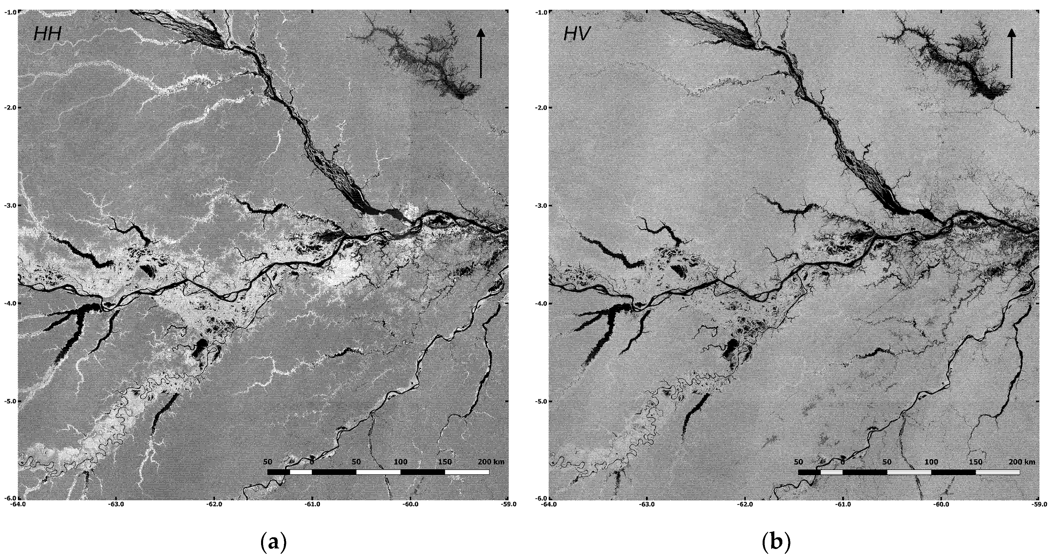
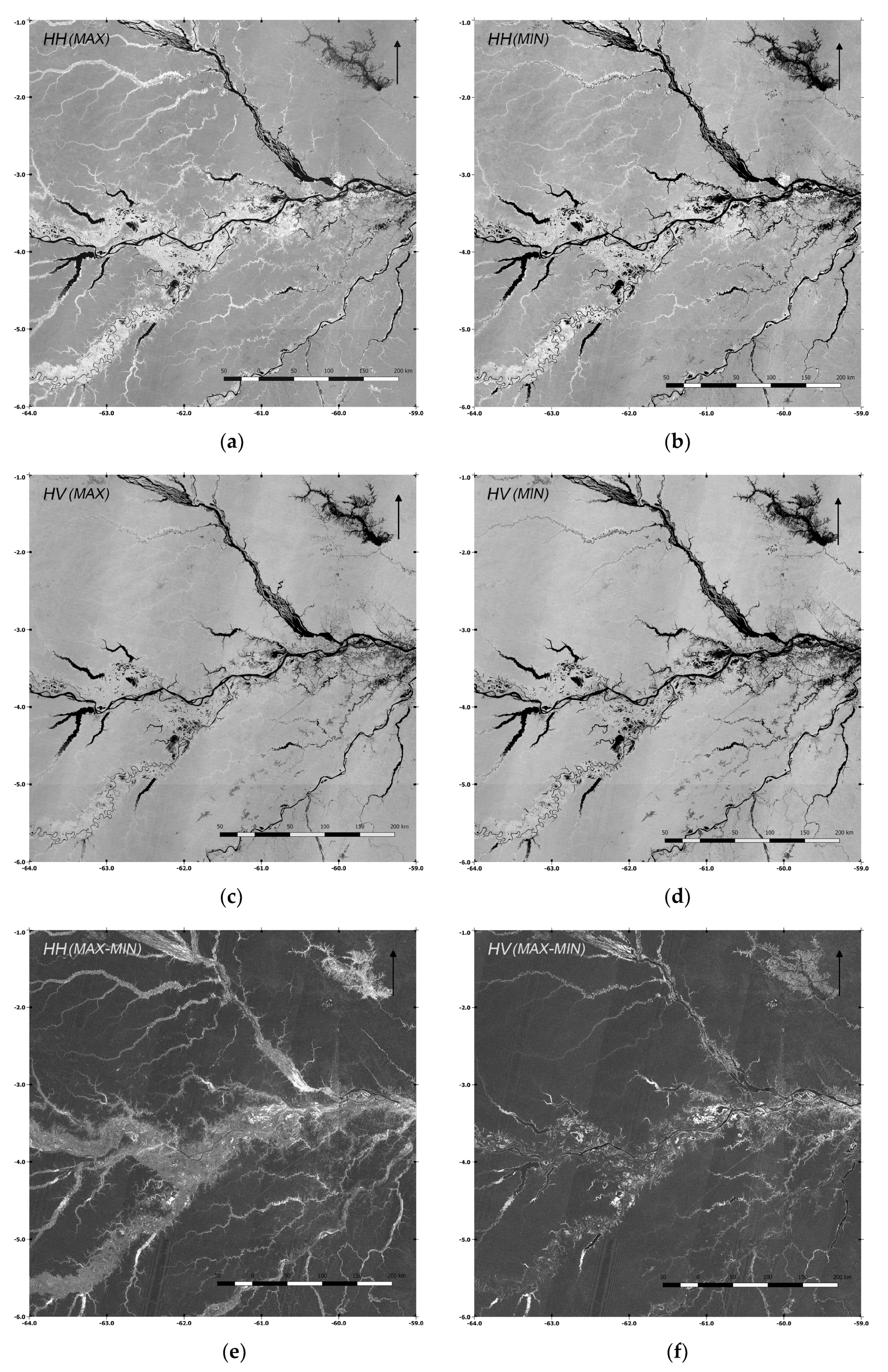
2.2.1. Generation of ALOS-2 PALSAR-2 Multi-Temporal Statistical Composite Imagery

Annual multi-temporal statistical composite imagery was produced from ALOS-2 PALSAR-2 ScanSAR time series to distinguish wetland from non-wetland areas. The composites generated covered three annual epochs: 2014/2015, 2015/2016 and 2016/2017, with each epoch starting in November and ending in October, in attempt to capture the beginning and end of the seasonal flood pulse across the entire basin for each annual flood season. The statistical composites created were: maximum HH and HV backscatter (MAX-HHYEAR and MAX-HVYEAR); minimum HH and HV backscatter (MIN-HHYEAR and MIN-HVYEAR) for each year; and the six corresponding difference images ((MAX−MIN)-HHYEAR and (MAX−MIN)-HVYEAR). Year = 14/15, 15/16 or 16/17).
Figure 3a,c show the maximum intensity images for HH-pol and HV-pol respectively, which represent the brightest pixels extracted across the 2016/2017 flood season time series. Figure 3b,d show the corresponding minimum intensity images for HH-pol and HV-pol respectively. Figure 3e,f show the MAX–MIN difference for HH-pol and HV-pol.
Bright areas in Figure 3e (HH-pol MAX-MIN difference) consequently represent areas of significant difference in HH backscatter between the maximum and minimum images. This can either indicate vegetation that becomes inundated during high water (low water: low HH backscatter; high water: high HH backscatter), or possible seasonal submergence of vegetation (low water: high HH backscatter; high water: low HH backscatter). This classification ambiguity can be resolved by using HV polarization data. As the HV polarized backscatter is sensitive to vegetation structure but not to inundation, bright areas in the HV-pol MAX–-MIN difference image in Figure 3f indicate areas also likely to be dominated by seasonally submerged vegetation (low water: high HV backscatter; high water: low HV backscatter). Inundated vegetation and seasonally submerged vegetation can thus be separated using both the HH and HV data.

2.2.2. Classification Algorithm

This study employs a decision tree method for classification. Building on methods developed by Martinez, et al. [3], vegetation and inundation classes were characterized based on knowledge of the L-band radar scattering behaviour of inundated vegetation. Four different classes were identified in the classifier (see Figure 4 and Figure 5):
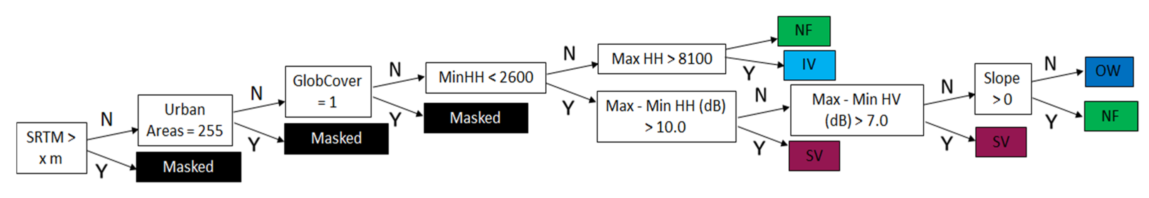
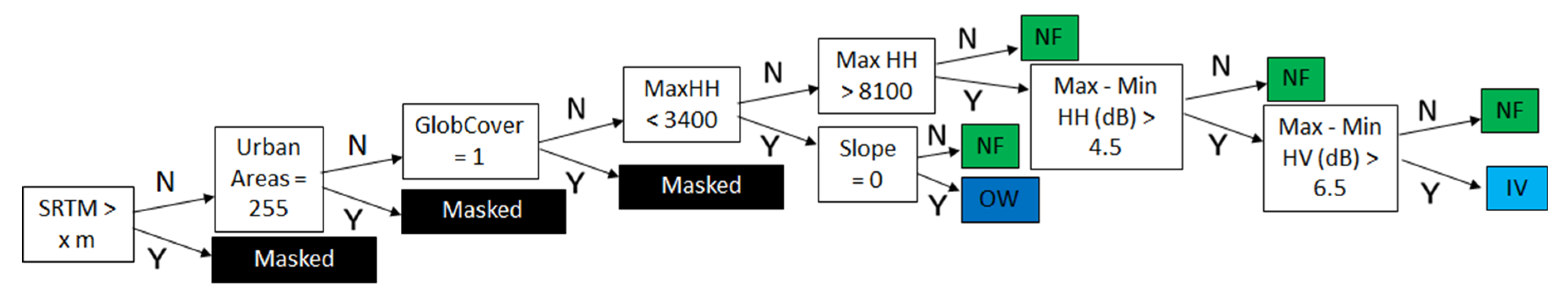
Inundated Vegetation (IV);
Seasonally Submerged Vegetation (SV);
Open Water (OW);
Non-Flooded Vegetation (NF).
The statistics for each class in the different statistical mosaics were extracted to determine optimal separation of the various classes. The range of the classes was examined over a ±1 sigma range to the mean DN or dB values. The thresholds applied in the classification were adjusted using the classification maps by Jensen et al. [16], Rosenqvist et al. [14], Hess, et al. [9,10] and Chapman et al. [12] to create thresholds suitable for application to all three years when used in the algorithm.
Seasonally submerged vegetation (SV) was defined as a region having a large difference in both the HH and HV backscatter between the maximum and minimum intensity images with the algorithm being optimized to be suitable across the entire basin.
As any changes in land cover occurring between data takes in the time series, such as deforestation or agriculture, display similar change signals in the difference images as the seasonal inundation classes, they were masked out to avoid misclassification. As all such areas could not be masked entirely with the ancillary data available; however (as the GlobCover and GUF datasets extended only to 2006 and 2012, respectively), residual areas were masked manually. For smaller regions of deforestation and agriculture, an elevation threshold was applied based on examination of algorithm performance, reducing the misclassified SV regions. Special care was taken to assure that IV classification was not compromised through this method of masking.

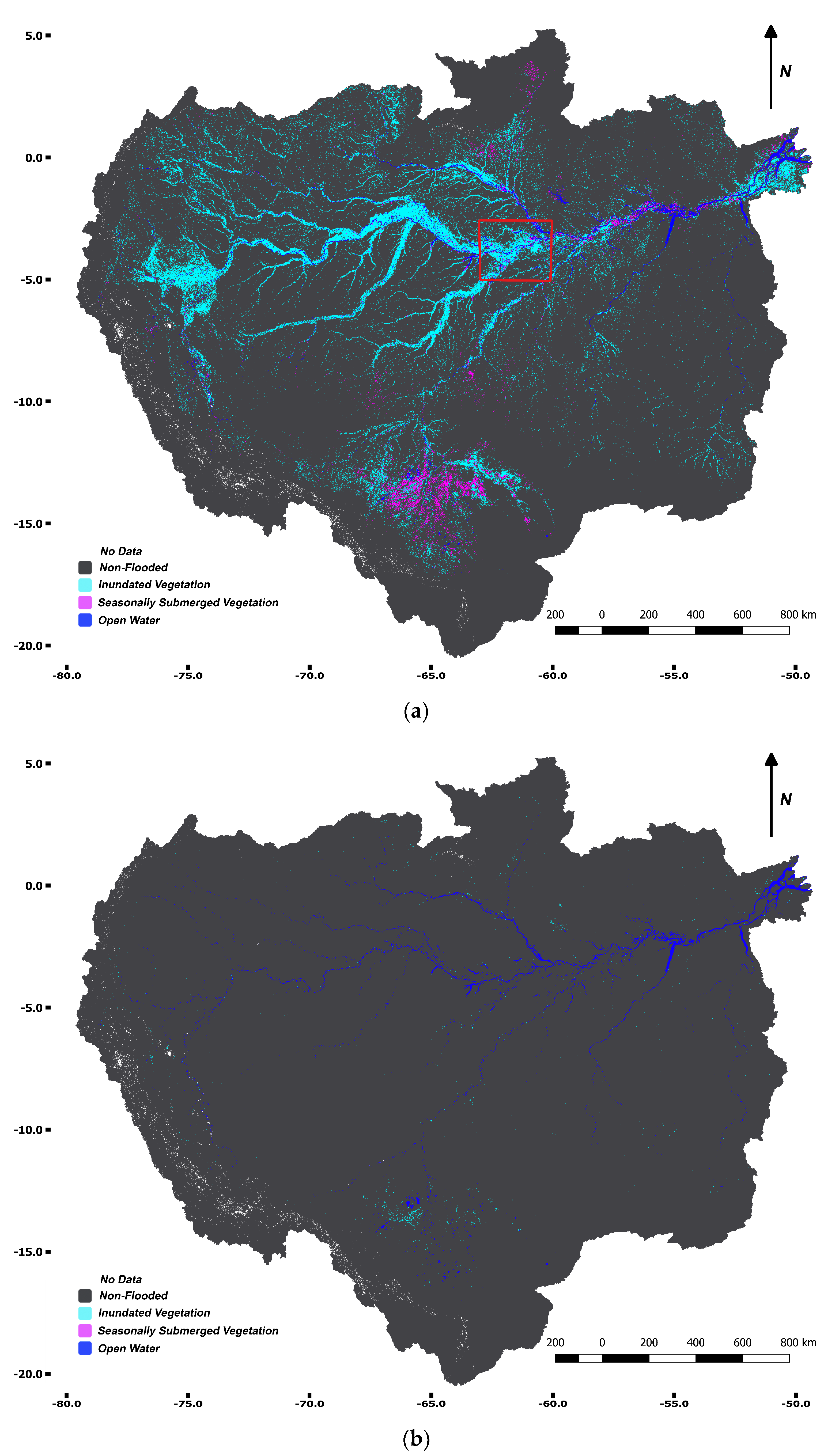
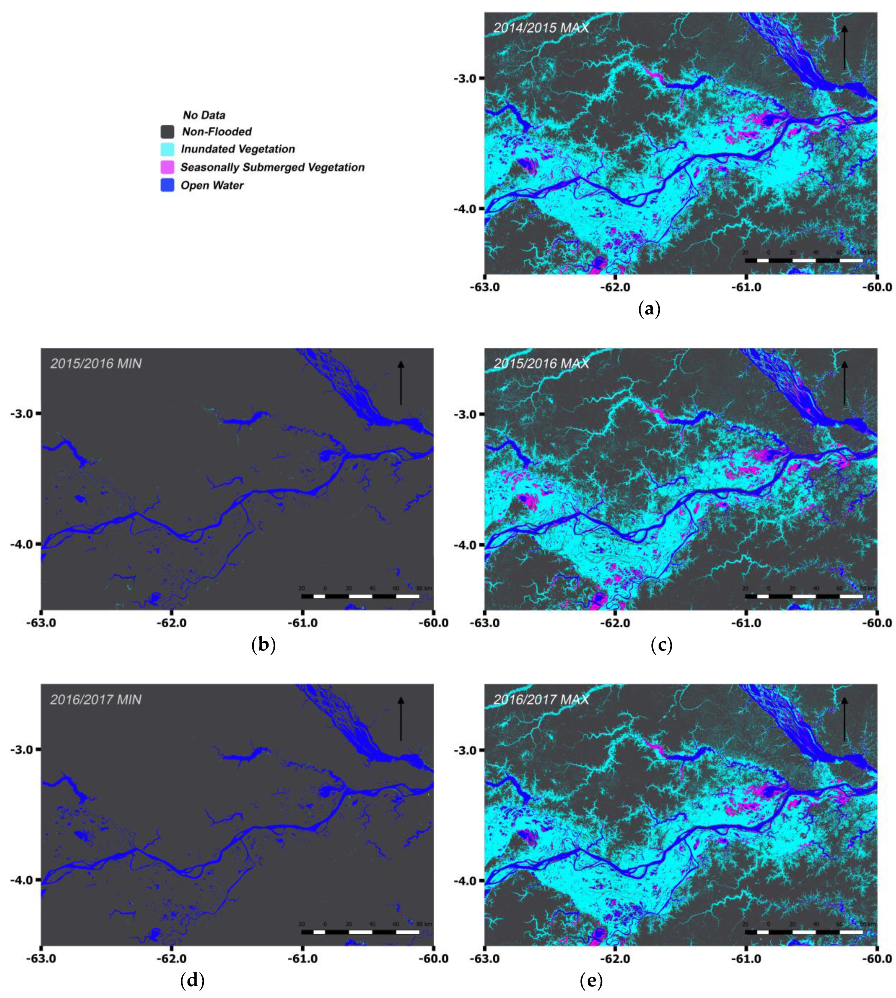
Maximum Inundation Extent Classification

Figure 4 shows the decision tree applied for classification of maximum inundation. The SRTM elevation threshold was adjusted within each sub-basin (Figure 2) to account for the differences in topography across the Amazon Basin. The MIN-HHYEAR (MinHH) image was used to separate OW and SV areas from other classes. as the largest area of open water is during the high-water season. The (MAX−MIN)-HVYEAR image was subsequently used to separate SV and OW. A slope image generated from the DEM was used in some sub-basins to separate the open water (zero slope) from bare ground/low vegetation, an approach also employed by Chapman et al. [12]. L-band HH-polarization is, as mentioned previously, highly sensitive to inundated vegetation as a result of the double bounce scattering effect, and the MAX-HHYEAR was thus used to separate the inundated vegetation from the non-flooded vegetation.

Minimum Inundation Extent Classification

The minimum inundation extent classification was limited to three classes: IV, OW and NF (as the seasonally submerged vegetation class, SV, by definition, was absent). The same statistical datasets and regions of interest (ROIs) used for the maximum inundation decision tree were used, and the thresholds were based on values extracted from the same ROIs as the maximum classification. The decision tree structure for classification of minimum inundation is presented in Figure 5.
The MAX-HHYEAR image reflects the minimum extent of open water, so it was used to separate OW regions. The (MAX−MIN)-HHYEAR image was used to distinguish NF from inundated or seasonally submerged areas. In the minimum inundation images, very small rivers, with widths similar to the ScanSAR pixel spacing (50 m) and smaller, could sometimes be misclassified as inundated due to the double-bounce scattering effect arising from trees along the banks of rivers that were not necessarily inundated. This classification artefact could not be corrected for.

3. Results

3.1. Classification

Figure 6a shows the full-basin maximum inundation extent classification map for the 2014/2015 hydrological year. Areas (pixels) classified as inundated (IV) or seasonally submerged (SV) vegetation have been identified as flooded in at least one of the (nine) acquisitions in the annual 2014/2015 time series stack. The map thus represents the maximum extent of flooding across the whole basin within the full hydrological year in question, regardless of the timing or duration of the flooding condition. The minimum inundation extent classification map for 2015/2016 (Figure 6b) consequently represents areas that have been identified as non-flooded (NF) in at least one acquisition in the November 2015–October 2016 time period. The total flooded area for the entire basin for the 2014/2015 maximum period was estimated to 528,741 km2, and the total flooded area for the 2015/2016 minimum period to 58,487 km2.
The classifications in Figure 6a,b above illustrate the vast extent of seasonal inundation in the Amazon Basin, annually flooding an area the size of Spain. The majority of the seasonally inundated varzea (white water) and igapò (black water) wetlands are located along the Amazon river main stem and its largest tributaries and in the sub-Andean wetlands in Peru. White water rivers include the Solimões, Madeira, Purus and Juruá rivers. They originate from the Andes and contain nutrient-rich sediments that result in the light-coloured water. Black water rivers have transparent water due to low volumes of suspended matter but are high in humic acids. Floodplains from black water rivers have a lower fertility than white water floodplains [2]. The largest areas of seasonally submerged vegetation (purple areas in the lower part of Figure 6a) occur in the Beni savannahs in the Bolivian part of the Madeira basin.
Figure 7 above shows the results for the three hydrological years for the central part of the Amazon/Solimões floodplain, indicated by the bounding box in Figure 6, with the Solimões and Purus river confluence in the central part of the images. Figures on the left are minimum inundation extent and figures on the right are the maximum inundation extent for each hydrological year.
Table 2 below presents the estimated areas of flooded, open water and submerged regions across the BL2 sub-basins for the years 2014–2017. The Amazon/Solimões floodplain (#3) had the largest percentage of inundated vegetation with respect to sub-basin area (29.1% in 2014/2015), followed by the Amazon Delta (#2) and Manacapuru (#13) basins that both had 20% inundation in the same year. The Amazon Delta (#2) also has the largest percentage of open water due to its proximity to the Atlantic Ocean. With the exception of the Bolivian savannahs, the percentage of submerged vegetation for each sub-basin is low, with an average of 0.8% for 2014/2015. In general, the 2015/2016 hydrological year exhibited less inundation across the basin than 2014/2015 and 2016/2017, with some exceptions being in the sub-basins north of the Amazon floodplain. Overall, the maximum inundation extent for the entire basin was 7% (412,824 sq. km) of the entire basin area in 2014/2015, 5.5% in 2015/2016 and 6% in 2016/2017. The percentage of submerged vegetation was 0.8–0.9%, and that of open water was 1% across all three years.
The minimum extent for 2014/2015 has been omitted in this study due to lack of consistent PALSAR-2 data for that period. For the following years, the minimum inundation extent for the entire basin was 0.1%, and the region of open water covered 0.9% of the basin.

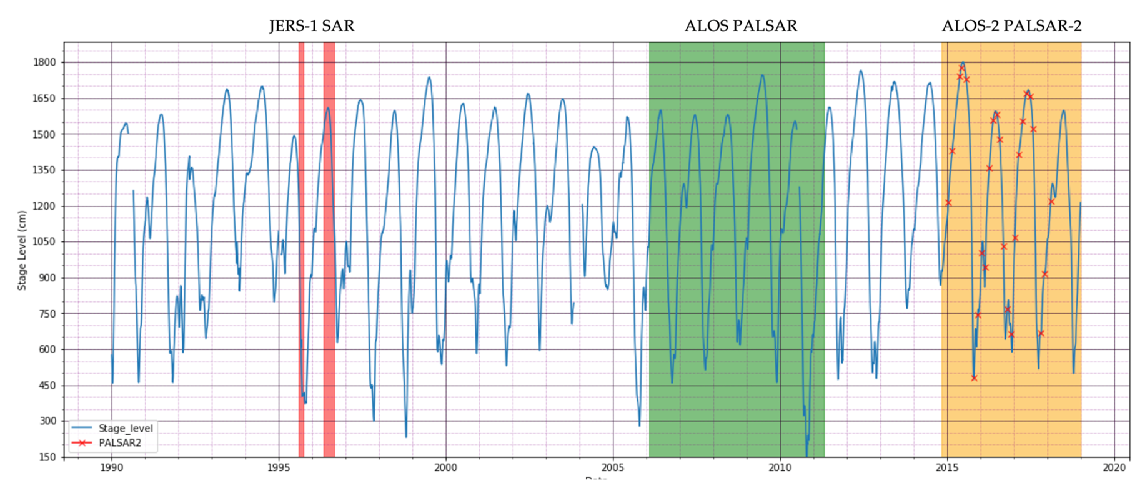
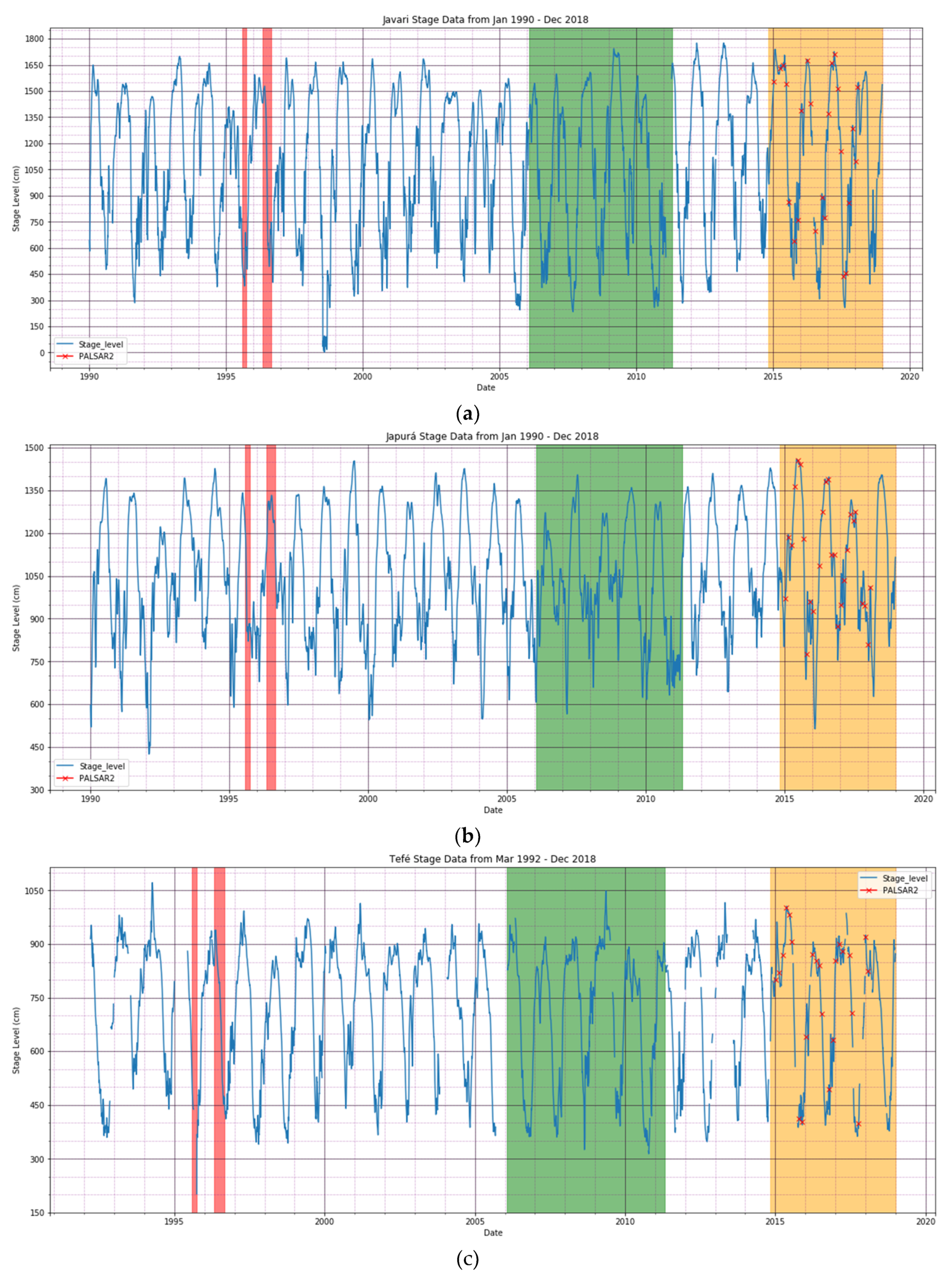
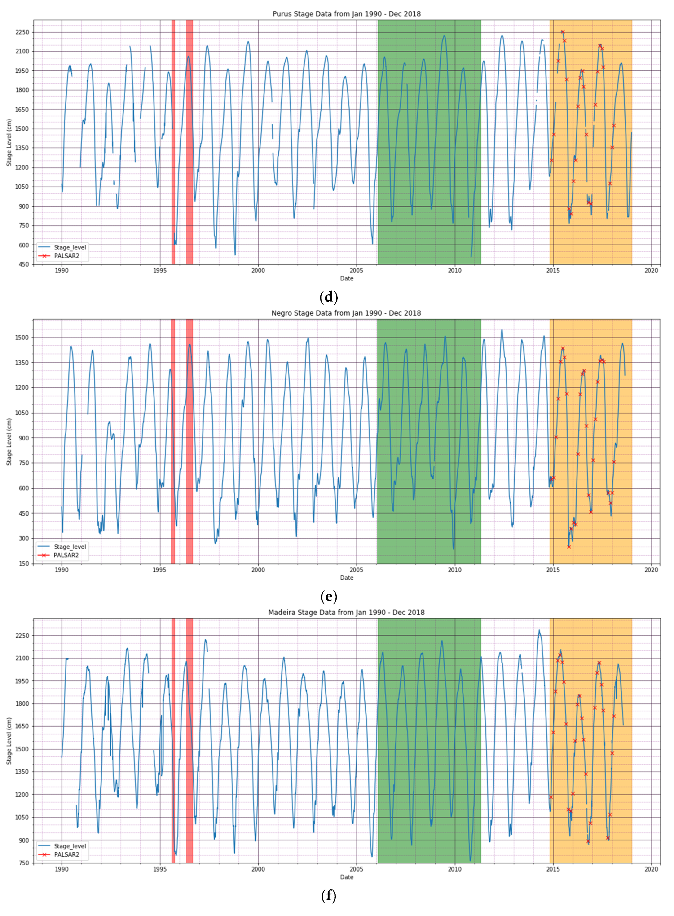
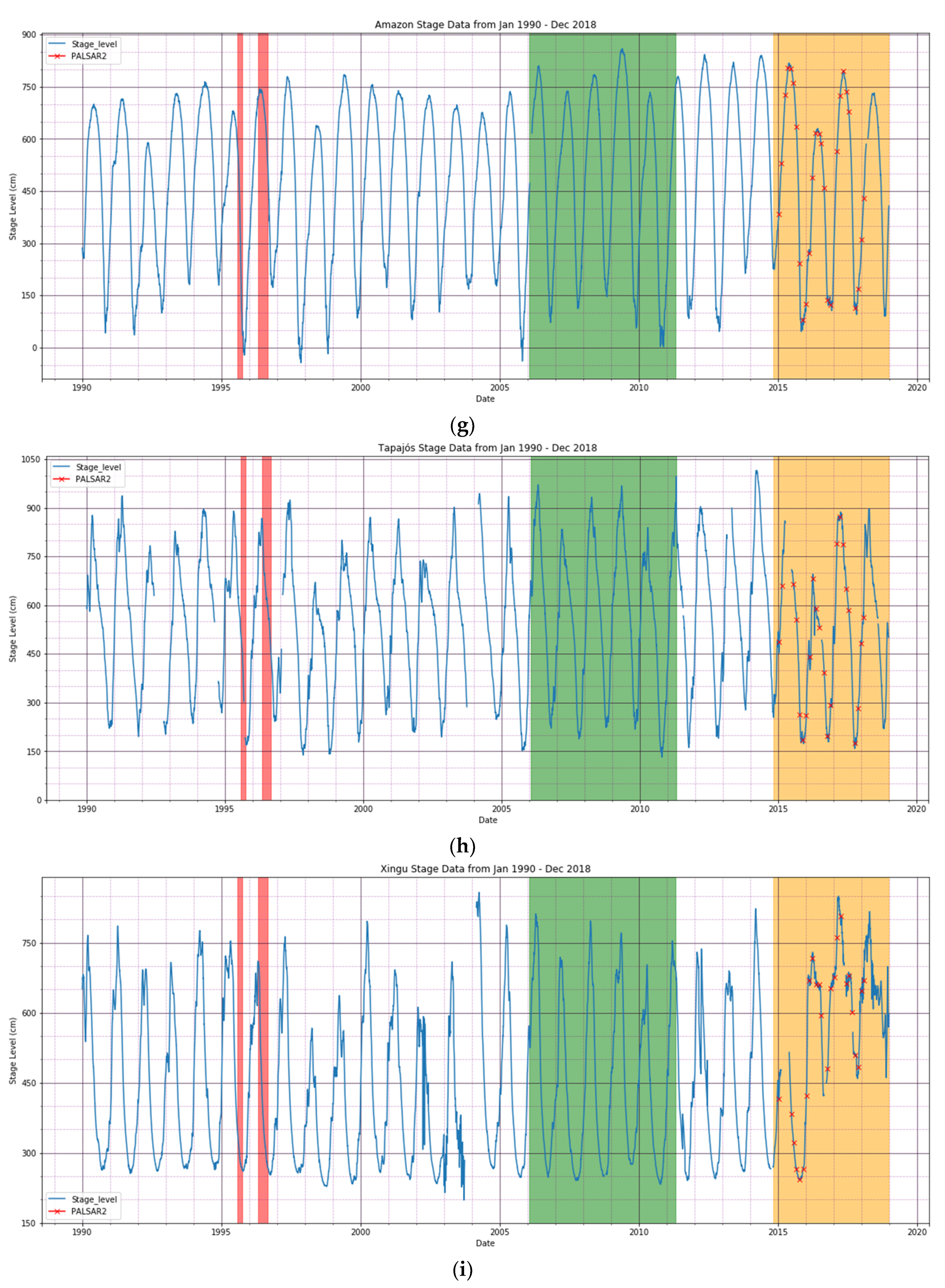
3.2. Temporal Representation of Annual Maximum and Minimum River Stages

In order to assess how accurately the inundation maps generated actually characterize the minimum and maximum inundation extents across the basin for each of the three hydrological years, we have assessed how well the PALSAR-2 acquisitions coincided with the high and low water extremes across the ten river gauge stations described above in Table 1 and Figure 2.
The diagram in Figure 8 below shows river height measurements since 1990 at the Itapeua gauge station (ANA code o-385) along the central part of the Solimões river, where water levels can differ more than 16 m between the high and low water seasons. The PALSAR-2 observation period is shown in yellow, with the acquisition dates for the ScanSAR data used in this study indicated with red crosses. Despite the rather coarse 42-day temporal repeat of the ScanSAR datatakes, the high-water extremes at this station have been captured within 6, 11 and 16 cm of the maximum levels recorded in 2015, 2016 and 2017, respectively. The low water extremes on the other hand, were captured less accurately, at 76 and 152 cm above the annual minimum levels recorded at Itapeua in 2015 and 2016.
Across the Amazon Basin, the differences between the annual extremes and the heights during the ScanSAR datatakes for each of the ten gauging stations are provided in Table 1 above (see figures in brackets). The corresponding stage height graphs for the other nine stations are given in Appendix A (Figure A1a–i).
The results indicate that the PALSAR-2 acquisitions provide a good representation of the high water extremes across the ten stations for all three years (two out of 28 datatakes within 50 cm of annual max), and fair representation of the low water the two years in question (14 out of 20 within 100 cm of the annual minimum).

4. Discussion: Comparison with Other Inundation Datasets

The lack of reference data on inundation extent is a major challenge associated with validation of wide-area inundation datasets such as the ones generated in this study. As standing water below a closed forest canopy cannot be detected by optical remote sensing or short wavelength (C-band, X-band) SAR sensors, and field measurements in situ only can provide point-wise or transect data, long-wavelength (L-band) SAR sensors remain the only means to provide geospatial information about forest inundation. It thus follows that the best we can do in terms of “proxy” validation is comparisons with other inundation datasets also generated by L-band SAR.

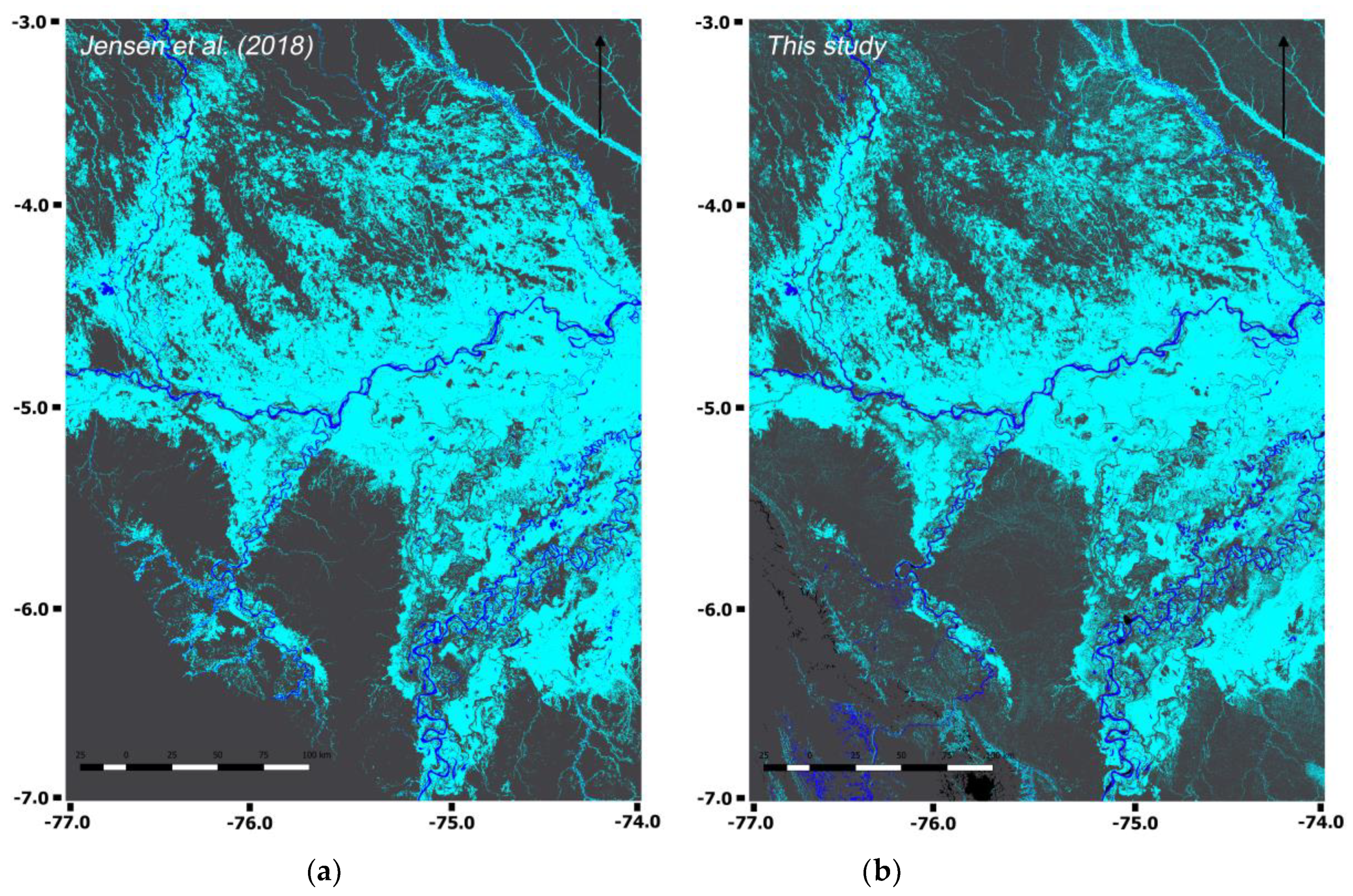
4.1. Local-Scale Comparison

A three-year maximum inundation extent map generated by Jensen et al. [16] over the Pacaya-Samiria National Reserve in Peru was used as proxy reference dataset to assess the robustness of the decision tree algorithm developed in this study for application across the entire Amazon Basin. The Jensen map was generated using PALSAR-2 ScanSAR time-series data that overlapped the data used in this study, spanning from November 2014 to February 2018, and accompanied by field validation in Peru.
To allow a more direct comparison with the Jensen map, a combined three-year maximum inundation extent image over the Pacaya-Samiria area was assembled from the three separate maximum inundation products generated in this study. The landcover classes were combined to represent only inundated vegetation, open water and non-flooded/masked/no data classes.
The two classified products are presented in Figure 9 and the corresponding confusion matrix in Table 3. The results suggest an overall agreement (86%) between the two classifications, with omissions and commissions in the inundated vegetation and open water classes in the order of 15–20%. The differences can be expected to be driven partly by the different classification algorithms and masking techniques used, but perhaps even more so due to the fact that the PALSAR-2 time series used for the two classifications differ slightly. The PALSAR-2 data used in this study end in October 2017, while the Jensen time series extends another four months until February 2018, thereby also comprising the start of the next high water season in the Pacaya-Samiria region, resulting in the fact that the two products cannot be assumed to represent identical inundation conditions.

4.2. Basin-Wide Comparison

4.2.1. Dataset Characteristics

The inundation maps generated by Hess et al. from JERS-1 SAR [9,10] and Chapman et al. from ALOS PALSAR [12] were used for a basin-wide comparison. Although the three datasets cover different time periods and use different class definitions, this presents an interesting opportunity to compare the classifications also at sub-basin scale across the 25 BL2 catchments defined by Venticinque et al. [26].
To accommodate a simple comparison between the datasets, the detailed and more numerous classes present in the JERS-1 classification by Hess et al. were combined to form the four main classes used in this study (i.e., IV, SV, OW and NF). As this study did not include macrophytes and did not distinguish between different vegetation types, as was carried out for the JERS-1 study; the macrophytes class in the JERS-1 study was therefore incorporated into the submerged vegetation class (SV), while the inundated shrub, woodland and forest classes were all combined into the inundated vegetation (IV) class.
Classes in the PALSAR-1 derived dataset by Chapman et al. included “occasionally flooded” and open water, and these were combined with the inundated vegetation (IV) and open water (OW) classes, respectively, for the maximum inundation extent. Similarly, occasionally flooded and occasionally open water classes defined in the PALSAR-1 dataset were associated with the non-flooded class (NF) in the minimum extent dataset.
It should be noted that the inundation figures for the JERS-1, PALSAR and PALSAR-2 products are not directly comparable, as each product represents a slightly different definition of inundation. The maps by Hess et al. are based on “snapshots” of the (September–December) 1995 low water and (May-Aug) 1996 high water extents, while the Chapman et al. product depicts the high water and low water averages during the 2006–2010 time period. The figures for this study used for this comparison, in turn represent the three-year combined maximum and minimum values.
As flood extents can vary significantly between years and between sub-basins across the Amazon, relative river gauge data from the ten ANA stations (in Table 1) are also provided in Table 4 and Table 5. For this study the stage values represent the water levels measured during actual PALSAR-2 acquisition dates, while for the Hess and Chapman maps (for which the exact SAR acquisition dates are not provided) the stage values indicate the station maximum and minimum readings for the respective acquisition periods, and thus only provide an approximate indication of the river levels during the JERS-1 and PALSAR acquisitions.

4.2.2. Observations

Table 4 below shows the high water/maximum estimates for the three products. The total area of the Amazon Basin used in this study is 5,954,414 km2, corresponding to the sum of the 25 BL2 sub-basins by Venticinque et al. [26].
An initial observation is that both this study and Chapman have mapped fewer inundated environments (IV, SV and OW) than that by Hess, despite the fact that maximum river heights measured during the PALSAR and PALSAR-2 observations along most gauging stations are similar or higher than the corresponding values during the JERS-1 observation period. The fractions of total flooding mapped by this study and Chapman et al. amount to 9.0% and 9.5%, respectively; compare that to 10.7% by Hess et al. The discrepancy is to the largest extent caused by the significantly different estimates in the (enormous) Madeira basin (#11), where the difference in total flooded area estimated by Chapman et al. and this study on one hand, and that by Hess et al. on the other, amounts to about 100,000 km2.
Excluding the Madeira basin (as well as the Amazon Delta (basin #2) which is only partially covered in the JERS-1 product), we note much closer correspondence between the three products, with total maximum flooded area (including IV, SV and OW) estimated at 414,000 km2, 441,000 km2 and 423,000 km2 for this study, Chapman et al. and Hess el al., respectively.
On a sub-basin level, we note that the Amazon/Solimões floodplain (Basin #3) has a greater percentage of inundated vegetation mapped by PALSAR-2 compared to the other datasets. This correlates well with the river stage data for Purus, Amazon and Solimões stations, where the maximum for 2015 is the highest among the four years gathered between PALSAR-2 and JERS-1. The station maximums among the three stations are also close in value with that of PALSAR-2, and the dates of the station maximum and PALSAR-2 acquisition dates for its maximum across the three years for Purus, Solimões and Amazon coincide very well. Basin #3 has a 10–20% lower inundation percentage for 2006–2011 compared to the other two decades.
The large Xingu basin (#25) shows very low (<1.5%) inundated vegetation regions for this study; while twice and three times greater by Chapman and by Hess, respectively Comparing this to the Xingu stage data, the maximum levels are lower for the sensors compared to the station’s values; and 2015 shows a very low stage level for the PALSAR-2 acquired date compared to the other years, but that is not reflected in the estimated inundation percentage in Table 4.
At the Negro station, the maximum levels for all sensors show a very close correspondence to the station level maximum. The maximum stage values for JERS-1 and the three years in this study are within 1 m of one another. The percentages of inundation in the Negro basin (#17) for the three years in this study range between 7.9 and 8.4%, and their similar inundation percentages correlate well with the similar stage values across the three years. The inundation percentage for JERS-1 is 11.0%, which is slightly higher than that from this study, despite the stage levels between the years being similar to one another.
Table 5 shows the low water/minimum estimates for the three products. We note an overall close correspondence between the PALSAR and PALSAR-2 classifications. This study’s “minimum extent” constitutes the lowest total flooded area estimate (1% or 57,000 km2), even though the PALSAR-2 datatakes did not manage to target the annual (2014–2017) minimum gauges very accurately. The Chapman study estimates the “average low water” at 1.6% (93,000 km2), mainly due to high estimates for Amazon/Solimões floodplain (and two of its small tributaries, #13 and #18). The JERS-1 “1995 low water” classification estimates total flooded areas at 4.8%.

5. Conclusions

This study has employed PALSAR-2 ScanSAR time series datasets along with ancillary data (SRTM, landcover maps) within a decision tree classification scheme to create three maximum and two minimum inundation extent datasets for the period 2014–2017 for the Amazon Basin. Comparisons with existing local and basin-wide inundation maps also generated by L-band SAR indicate comparable results for inundated areas during the maximum inundation conditions, and uniquely low estimates of minimum inundation extents. Although some available ancillary datasets may differ across regions, the general technique should be transferable to other flood pulse-dominated wetlands, albeit with corresponding adjustments made to the region-specific thresholds supporting implementation of the decision tree. In principle, this architecture should be applicable to other types of wetlands ecosystems, although some aspects of implementation need to be revisited.
Comparisons between the stage data across the basin and PALSAR-2 acquisition dates/periods show that the sensor has captured the nature of the maximum and minimum flooding across the basin but has not captured the precise maximum and minimum inundation levels that have been recorded in the stage data. Better accuracy of the inundation datasets for all sensors would have been possible with higher temporal fidelity in the SAR acquisition and in mosaic assembly. Some limitations included the lack of overlapping temporal ancillary data to effectively mask present urban, agriculture and deforested areas, and a lack of in situ data over multiple regions across the basin. Availability of these datasets would have helped create a more accurate inundation product.
Future work will involve the use of the inundation extent datasets from this study to generate inundation duration products over the entire basin. The inundation extent products will be used as a mask to delineate the areas of maximum and minimum inundation extents. We will be extending the time period of the inundation duration datasets to include ScanSAR data until 2018.

6. Data Access

The classification maps generated within this study are available for public download under a Creative Commons (CC BY 4.0) license at the NASA Earth System Data Record (ESDR) at the Alaska Satellite Facility Distributed Active Archive Center (DAAC) [13].

Author Contributions

Conceptualization, J.R. and A.R.; methodology, J.R. and K.J.; software, J.R. and K.J.; validation, J.R. and K.J.; formal analysis, J.R. and A.R.; data curation, J.R.; writing—original draft preparation, J.R.; writing—review and editing, A.R., K.M. and K.J.; visualization, J.R.; supervision, K.M. and A.R.; project administration, K.M.; funding acquisition, K.M. All authors have read and agreed to the published version of the manuscript.

Funding

This research was supported by funding from the NASA Making Earth Science Data Records for Use in Research Environments (MEaSUREs) program under grant number NNX11AQ39G, and from the NASA Biodiversity and Ecological Forecasting Program and NSF’s Dimensions of Biodiversity Program under grant DEB-1343578.

Acknowledgments

This research was undertaken in part within the framework of the ALOS Kyoto and Carbon Initiative. ALOS-2 PALSAR-2 ScanSAR mosaics were provided by JAXA EORC.

Conflicts of Interest

The authors declare no conflict of interest.

Appendix A

River Stage Data across the Amazon Basin (Source: Agência Nacional de Águas [27])
Figure A1. (a) River stages 1990–2018. Station o-326, Estirão do Repouso, Rio Javari (S4.341°/W70.906°); (b) 1990–2018. Station o-375, Acanaui, Rio Japurá (S1.821°/W66.600°); (c) 1992-2018. o-381, Estirão da Santa Cruz, Rio Tefé (S4.292°/W65.202°). (d) 1990–2018. o-437, Paricatuna, Rio Purus (S4.409°/W61.899°); (e) 1990–2018. o-497, Moura, Rio Negro (S1.457°/W61.635°); (f) 1990–2018. o-618, Borba, Rio Madeira (S4.389°/W59.599°). (g) 1990–2018. o-681, Óbidos, Rio Amazonas (S1.919°/W55.513°); (h) 1990–2018. o-733, Itaituba, Rio Tapajós (S4.276°/W55.982°); (i) 1990–2018. o-811, Altamira, Rio Xingu (S3.215°/W52.212°).
Remotesensing 12 01326 g0a1aRemotesensing 12 01326 g0a1bRemotesensing 12 01326 g0a1c

References

  1. Junk, W.J.; Bayley, P.B.; Sparks, R.E. The flood pulse concept in river-floodplain systems. Can. Spec. Publ. Fish. Aquat. Sci. 1989, 106, 110–127. [Google Scholar]
  2. Junk, W.J.; Piedade, M.T.; Wittmann, F.; Schöngart, J.; Parolin, P. Amazonian Floodplain Frests: Ecophysiology, Biodiversity and Sustainable Management; Springer Science & Business Media: Berlin, Germany, 2010; Volume 210. [Google Scholar]
  3. Martinez, J.; Le Toan, T. Mapping of flood dynamics and spatial distribution of vegetation in the Amazon floodplain using multitemporal SAR data. Remote Sens. Environ. 2007, 108, 209–223. [Google Scholar] [CrossRef]
  4. Richey, J.E.; Melack, J.M.; Aufdenkampe, A.K.; Ballester, V.M.; Hess, L.L. Outgassing from Amazonian rivers and wetlands as a large tropical source of atmospheric CO2. Nature 2002, 416, 617. [Google Scholar] [CrossRef] [PubMed]
  5. MacDonald, H.; Waite, W.; Demarcke, J. Use of Seasat Satellite Radar Imagery for the Detection of Standing Water Beneath Forest Vegetation; NASA: Washington, DC, USA, 1981. [Google Scholar]
  6. Rosenqvist, A.; Shimada, M.; Chapman, B.; Freeman, A.; De Grandi, G.; Saatchi, S.; Rauste, Y. The global rain forest mapping project-a review. Int. J. Remote Sens. 2000, 21, 1375–1387. [Google Scholar] [CrossRef]
  7. Freeman, A.; Chapman, B.; Siqueira, P. The JERS-1 Amazon Multi-season Mapping Study (JAMMS): Science objectives and implications for future missions. Int. J. Remote Sens. 2002, 23, 1447–1460. [Google Scholar] [CrossRef]
  8. Shimada, M.; Ohtaki, T. Generating large-scale high-quality SAR mosaic datasets: Application to PALSAR data for global monitoring. IEEE J. Sel. Top. Appl. Earth Obs. Remote Sens. 2010, 3, 637–656. [Google Scholar] [CrossRef]
  9. Hess, L.L.; Melack, J.M.; Novo, E.M.; Barbosa, C.C.; Gastil, M. Dual-season mapping of wetland inundation and vegetation for the central Amazon basin. Remote Sens. Environ. 2003, 87, 404–428. [Google Scholar] [CrossRef]
  10. Hess, L.L.; Melack, J.M.; Affonso, A.G.; Barbosa, C.; Gastil-Buhl, M.; Novo, E.M. Wetlands of the lowland Amazon basin: Extent, vegetative cover, and dual-season inundated area as mapped with JERS-1 synthetic aperture radar. Wetlands 2015, 35, 745–756. [Google Scholar] [CrossRef]
  11. Melack, J.M.; Hess, L.L. Remote Sensing of the Distribution and Extent of Wetlands in the Amazon Basin. In Amazonian Floodplain Forests; Springer: Berlin, Germany, 2010; pp. 43–59. [Google Scholar]
  12. Chapman, B.; McDonald, K.; Shimada, M.; Rosenqvist, A.; Schroeder, R.; Hess, L. Mapping regional inundation with spaceborne L-band SAR. Remote Sens. 2015, 7, 5440–5470. [Google Scholar] [CrossRef] [Green Version]
  13. NASA Earth System Data Record (ESDR) at the Alaska Satellite Facility Distributed Active Archive Center (DAAC). Available online: https://asf.alaska.edu/data-sets/derived-data-sets/wetlands-measures/ (accessed on 16 April 2020).
  14. Rosenqvist, A.; Forsberg, B.R.; Pimentel, T.; Rauste, Y.A.; Richey, J.E. The use of spaceborne radar data to model inundation patterns and trace gas emissions in the central Amazon floodplain. Int. J. Remote Sens. 2002, 23, 1303–1328. [Google Scholar] [CrossRef]
  15. Arnesen, A.S.; Silva, T.S.F.; Hess, L.L.; Novo, E.M.L.M.; Rudorff, C.M.; Chapman, B.D.; McDonald, K.C. Monitoring flood extent in the lower Amazon River floodplain using ALOS/PALSAR ScanSAR images. Remote Sens. Environ. 2013, 130, 51–61. [Google Scholar] [CrossRef]
  16. Jensen, K.; McDonald, K.; Podest, E.; Rodriguez-Alvarez, N.; Horna, V.; Steiner, N. Assessing L-band GNSS-reflectometry and imaging radar for detecting sub-canopy inundation dynamics in a tropical wetlands complex. Remote Sens. 2018, 10, 1431. [Google Scholar] [CrossRef] [Green Version]
  17. Evans, T.L.; Costa, M.; Telmer, K.; Silva, T.S.F. Using ALOS/PALSAR and RADARSAT-2 to Map Land Cover and Seasonal Inundation in the Brazilian Pantanal. IEEE J. Sel. Top. Appl. Earth Obs. Remote Sens. 2010, 3, 560–575. [Google Scholar] [CrossRef]
  18. Rosenqvist, A.; Birkett, C. Evaluation of the JERS-1 SAR mosaics for hydrological applications in the Congo River basin. Int. J. Remote Sens. 2002, 23, 1283–1302. [Google Scholar] [CrossRef]
  19. Hidayat, H.; Hoekman, D.H. Flood occurrence mapping of the middle Mahakam lowland area using satellite radar. Hydrol. Earth Syst. Sci. 2012, 16, 1805–1816. [Google Scholar] [CrossRef] [Green Version]
  20. ALOS-2 PALSAR-2 Basic Observation Scenatio website, Japan Aerospace Exploration Agency. Available online: www.eorc.jaxa.jp/ALOS-2/en/obs/pal2_obs_guide.htm (accessed on 16 April 2020).
  21. Rosenqvist, A.; Shimada, M.; Suzuki, S.; Ohgushi, F.; Tadono, T.; Watanabe, M.; Tsuzuku, K.; Watanabe, T.; Kamijo, S.; Aoki, E. Operational performance of the ALOS global systematic acquisition strategy and observation plans for ALOS-2 PALSAR-2. Remote Sens. Environ. 2014, 155, 3–12. [Google Scholar] [CrossRef]
  22. Rosenqvist, A.; Rebelo, L.M.; Costa, M. The ALOS Kyoto & Carbon Initiative: Enabling the mapping, monitoring and assessment of globally important wetlands. Wetl. Ecol. Manag. 2015, 23. [Google Scholar]
  23. Farr, T.G.; Kobrick, M. Shuttle Radar Topography Mission produces a wealth of data. Eostrans. Am. Geophys. Union 2000, 81, 583–585. [Google Scholar] [CrossRef]
  24. Esch, T.; Heldens, W.; Hirner, A.; Keil, M.; Marconcini, M.; Roth, A.; Zeidler, J.; Dech, S.; Strano, E. Breaking new ground in mapping human settlements from space–The Global Urban Footprint. Isprs J. Photogramm. Remote Sens. 2017, 134, 30–42. [Google Scholar] [CrossRef] [Green Version]
  25. Arino, O. GlobCover: ESA service for global land cover from MERIS. IEEE Int. Geosci. Remote Sens. Symp. (Igarss’07), Barc 2007, 2412–2415. [Google Scholar]
  26. Venticinque, E.; Forsberg, B.; Barthem, R.; Petry, P.; Hess, L.; Mercado, A.; Cañas, C.; Montoya, M.; Durigan, C.; Goulding, M. An explicit GIS-based river basin framework for aquatic ecosystem conservation in the Amazon. Earth Syst. Sci. Data 2016, 8, 651. [Google Scholar] [CrossRef] [Green Version]
  27. Hidroweb, Agência Nacional de Águas. Available online: http://www.snirh.gov.br/hidroweb/publico/apresentacao.jsf (accessed on 16 April 2020).
Figure 1. ALOS-2 PALSAR-2 ScanSAR 5° × 5° tile composite (PALSAR-2 cycle 27, July 2017) over the Central Amazon Basin. (a) HH-polarization. (b) HV-polarization (© JAXA).
Remotesensing 12 01326 g001
Figure 2. Amazon River basin catchment areas, basin level 2 (major tributary basins) as defined by Venticinque et al. [26] (Background: Google Earth).
Remotesensing 12 01326 g002
Figure 3. Statistical images derived from ALOS-2 PALSAR-2 ScanSAR cycles for the 2016/2017 flood season. (a) Maximum HH-pol backscatter image. Inundated vegetation can be seen as very bright pixels. (b) Minimum HH-pol image. (c) Maximum HV-pol image. (d) Minimum HV-pol image. (e) HH-pol difference (MAX–MIN) image. (f) HV-pol difference (MAX–MIN) image. Areas exhibiting large seasonal variations in backscatter appear bright in (e) and (f). (© JAXA).
Remotesensing 12 01326 g003
Figure 4. Decision tree applied to derive classification for maximum inundation. IV: inundated vegetation, SV: seasonally submerged vegetation, OW: open water, NF: non-flooded vegetation. The SRTM elevation threshold was adjusted for each sub-basin to account for variations in elevation and topography amongst the sub-basins. Ancillary data on urban areas and land cover were used to mask anthropogenic areas. The elevation and anthropogenic areas are all under the “masked” class.
Remotesensing 12 01326 g004
Figure 5. Decision tree for minimum inundation classification. IV: inundated vegetation, OW: open water, NF: non-flooded vegetation.
Remotesensing 12 01326 g005
Figure 6. (a) Full-basin maximum inundation extent for 2014/2015. Light blue: inundated vegetation; purple: submerged vegetation; blue: open water; grey: non-flooded; white: no data. The red box indicates the region shown in Figure 7. (b) Full basin minimum inundation extent classification for the hydrological year 2015/2016. Light blue: inundated vegetation; purple: submerged vegetation; blue: open water; grey: non-flooded; white: no data.
Remotesensing 12 01326 g006
Figure 7. Minimum and maximum inundation extents over three hydrological years covering the region in the bounding box in Figure 6. Light blue: inundated vegetation, blue: open water; purple: seasonally submerged vegetation; grey: non-flooded; white: no data. (a) 2014/2015, (b,c) 2015/2016 and (d,e) 2016/2017.
Remotesensing 12 01326 g007
Figure 8. River stages 1990–2018. Station o-385, Itapeua, Rio Solimões (S4.058°/W63.028°). Red, green and yellow fields indicate JERS-1 SAR, ALOS-PALSAR and ALOS-2 PALSAR-2 acquisition periods, respectively. Red crosses indicate PALSAR-2 acquisition dates and illustrate how well the annual maximum and minimum inundation levels around the gauge station were captured in the PALSAR-2 data.
Remotesensing 12 01326 g008
Figure 9. Classification images of Pacaya-Samiria. Light blue: inundated vegetation; blue: open water; grey: non-flooded/masked areas/no data. (a) Classification by Jensen et al. [16]. (b) Classification in this study.
Remotesensing 12 01326 g009
Table 1. River height gauging stations used to assess ScanSAR data representations of annual maximum and minimum flooding conditions across the basin. Values indicate the highest and lowest annual river stages recorded during the ALOS-2 PALSAR-2 acquisitions. Figures in brackets indicate the difference corresponding to the station maximum or minimum stage that same hydrological year. All values are in meters (Source: Agência Nacional de Águas, ANA).
ANA CodeStation NameBL2 Drainage Basin (basin# in Fig. 2)LatLon2014/20152015/20162016/2017
MaxMinMaxMinMax
o-326Est. do RepousoJavari (basin #8)−4.341−70.90613.18 (−1.87)4.63 (+3.90)14.42 (−0.04)2.04 (+1.81)14.77 (−0.15)
o-375AcanauiJapurá (#6)−1.821−66.60010.30 (−0.05)5.01 (+4.12)9.65 (−0.07)5.30 (+0.98)8.42 (−0.50)
o-381Est. da Santa CruzTefé (#21)−4.292−65.2026.88 (−0.04)1.80 (+1.01)5.58 (−0.34)0.84 (+0.36)5.66 (−1.06)
o-385ItapeuaSolimões Floodplain (#3)−4.058−63.02816.64 (−0.06)5.32 (+0.76)14.52 (−0.11)5.38 (+1.52)15.37 (−0.16)
o-437ParicatubaPurus (#19)−4.409−61.89917.46 (−0.03)4.10 (+0.87)14.38 (−0.14)5.68 (+2.75)16.35 (−0.11)
o-497MouraNegro (#17)−1.457−61.63512.00 (−0.01)1.60 (+1.11)10.66 (−0.03)2.78 (+0.81)11.28 (−0.29)
o-618BorbaMadeira (#11)−4.389−59.59913.58 (−0.35)1.31 (+0.21)10.88 (−0.07)1.55 (+0.20)13.07 (−0.07)
o-681ÓbidosAmazonas Floodplain (#3)−1.919−55.5138.48 (−0.14)1.69 (+0.22)6.61 (−0.13)1.57 (+0.18)8.39 (−0.01)
o-733ItaitubaTapajós (#20)−4.276−55.982N/A0.59 (+0.12)5.45 (−0.18)0.38 (+0.12)7.40 (−0.15)
o-811AltamiraXingu (#25)−3.215−52.212N/A2.23 (+0.57)5.18 (−0.13)2.84 (+0.22)6.08 (−0.43)
Table 2. Maximum and minimum inundation area estimates Nov. 2014 – Oct 2017 for Amazon basin tributary rivers, Basin Level 2 as per Venticinque et al. [26].
2014/20152015/20162016/2017
MAXMINMAXMINMAX
#Basin Name (BL2)Basin Area (sq. km)Inund. VegSubm. Veg.Open WaterTOTAL FloodedInund. VegOpen WaterTOTAL FloodedInund. VegSubm. Veg.Open WaterTOTAL FloodedInund. VegOpen WaterTOTAL FloodedInund. VegSubm. Veg.Open WaterTOTAL Flooded
1 Abacaxis 126,98576614191260934078108311605314475123870275611431199678433912718395
2Amazon Delta67,86813,8732186882024,8802618629889011,9012649855523,1041818601878213,4092695837324,478
3Amazonas/Solimões Floodplain255,04374,171813819,243101,55228516,14916,43459,00810,05117,07886,13718517,07117,25666,007767019,05992,736
4 Curuá-Una 30,670136931424322022337122124712112133411814466
5 Ica/Putumayo 118,24015,36120976316,3332763566215,60728375316,6421263564712,44825275513,454
6Japurá252,81018,653538147720,668661274134018,883679147021,031411270131115,658470146417,591
7 Jari 134,108328322587359510764172365326195400984561403833250874170
8 Javari 107,60551048218453701347604346136193467519416046191521694940
9 Juruá189,10118,082528126519,8753445849210,766420131812,5035146751813,702423142215,547
10 Jutaí89,1006104137298654011125135394715129143882111713849711872585416
11 Madeira 1,323,67963,05430,468640899,93028665767863332,01524,871651663,4034233578410,01739,97728,428646774,871
12 Madeirinha 37,0913588218581438713286300230519754430471631433032491825643996
13 Manacapuru 11,327235814231428141226527717031073082118527427919781093242410
14 Marañón 361,88536,803631204439,4774611092155333,924979201836,9213371131146835,476733204238,252
15 Napo 100,845992411449710,5351737739491431934899825938839784371434899069
16Natay16,721931533969213151173183112231151699311341039
17 Negro 716,10356,7954954646068,2097445565630959,7984269658470,6514205835625558,8062369699468,169
18 Piorini 840214814614516721105105106366110123901381381008231601191
19 Purus 368,24030,534192786633,32716668585219,697135884421,8989171881023,031118288525,098
20 Tapajós 494,41287452414112,888156401041665054039148968141412142625820230278849
21 Tefé-Urucu59,87839692771046529312954967270220610723980210201023285614311334132
22 Trombetas 149,9763545287529436144434479340139651743151845247030812415353857
23 Uatumā73,29522263101411394828336064231991944923885174244412213104811174378
24 Ucayali 353,92219,813930258123,3242951562185715,015892248818,3952621525178719,229908231722,454
25 Xingu 507,1086629325809213168240425723920125066426172242926015198025567754
Total (sq. km)5,954,414412,82452,87063,048528,741614552,34358,487327,87248,97459,436436,282639553,97260,367353,11848,07661,517462,711
Table 3. Confusion matrix of the two decision tree classifications over Pacaya-Samiria National Reserve by Jensen et al. (2018) and this study. Values are in km2.
This Study
Inund. Veg.Open WaterNon-flooded/No Data Total [sq. km]Comm. error
Jensen et al. (2018)Inundated Veg.45,62617310,38156,18119%
Open Water1592456525314022%
Non-flooded/No Data796947171,19279,63311%
Total [sq. km]53,755310182,098138,953
Omission error15%21%13%Overall agreement: 86%
Table 4. Comparison of Amazon Basin high water/maximum inundation maps 1996–2017 by Hess et al. [8,9], Chapman et al. [11] and this study.
JERS-1 SAR (Hess et. al. 2003 & 2015)ALOS PALSAR (Chapman et. al. 2015)ALOS-2 PALSAR-2 (This study)
1996 HIGH Water Extent2006-2010 AVERAGE HIGH Water Extent2014-2017 MAXIMUM Extent
#Basin Name (BL2)Basin Area (sq. km)1996 MAX Gauge (m)Inund. VegSubm. Veg.Open WaterTOTAL Flooded2006-2010 MAX Gauge (m)Inund. VegSubm. Veg.Open WaterTOTAL FloodedPALSAR-2 MAX Gauge (m)Inund. VegSubm. Veg.Open WaterTOTAL Flooded
1 Abacaxis 126,985 4.29%0.13%1.31%5.7% 5.32%N/A1.16%6.5% 6.03%0.37%1.00%7.4%
2Amazon Delta67,868 N/AN/AN/AN/A 24.28%N/A4.90%29.2% 20.44%3.22%13.00%36.7%
3 Amazonas/Solimões Floodplain255,043o-385: 14.78
o-681: 7.88
26.42%3.71%9.48%39.6%o-385: 16.14
o-681: 9.04
17.30%N/A9.22%26.5%o-385: 16.64
o-681: 8.48
29.08%3.94%7.55%40.6%
4 Curuá-Una 30,670 1.41%0.05%0.08%1.5% 2.93%N/A1.92%4.8% 1.10%0.40%0.05%1.6%
5 Ica/Putumayo 118,240 11.78%0.68%0.89%13.3% 10.78%N/A0.99%11.8% 13.20%0.24%0.65%14.1%
6Japurá252,8109.087.36%0.70%0.78%8.8%9.809.21%N/A2.92%12.1%10.307.47%0.27%0.58%8.3%
7 Jari 134,108 1.51%0.03%0.06%1.6% 4.98%N/A0.55%5.5% 2.86%0.19%0.07%3.1%
8 Javari 107,60513.613.15%0.26%0.06%3.5%15.093.89%N/A0.11%4.0%14.774.74%0.14%0.18%5.1%
9 Juruá189,101 6.44%0.75%0.29%7.5% 6.84%N/A0.38%7.2% 9.56%0.28%0.75%10.6%
10 Jutaí89,100 6.36%0.59%0.17%7.1% 7.74%N/A0.08%7.8% 6.85%0.21%0.34%7.4%
11 Madeira 1,323,67913.167.40%6.99%1.17%15.6%14.524.68%N/A3.45%8.1%13.584.76%2.30%0.49%7.6%
12 Madeirinha 37,091 8.86%0.22%1.22%10.3% 6.38%N/A0.87%7.3% 9.67%0.59%1.57%11.8%
13 Manacapuru 11,327 9.32%0.18%3.16%12.7% 9.23%N/A2.55%11.8% 20.82%1.25%2.86%24.9%
14 Marañón 361,885 7.92%0.98%0.34%9.2% 6.71%N/A1.06%7.8% 10.17%0.27%0.56%11.0%
15 Napo 100,845 6.19%0.69%0.75%7.6% 8.30%N/A0.90%9.2% 9.84%0.19%0.49%10.5%
16Natay16,721 4.56%0.39%0.05%5.0% 3.47%N/A0.09%3.6% 7.02%0.11%0.21%7.3%
17 Negro 716,10312.2110.98%0.40%1.37%12.8%12.7111.44%N/A1.42%12.9%12.008.35%0.69%0.98%10.0%
18 Piorini 8402 9.10%0.13%2.12%11.3% 8.83%N/A1.44%10.3% 17.63%0.79%1.90%20.3%
19 Purus 368,24015.526.02%0.58%0.44%7.0%17.145.95%N/A0.96%6.9%17.468.29%0.52%0.24%9.1%
20 Tapajós 494,4127.352.54%0.06%0.96%3.6%8.653.05%N/A3.57%6.6%7.401.77%0.00%0.84%2.6%
21 Tefé-Urucu59,8786.256.28%0.07%1.98%8.3%7.354.66%N/A1.79%6.5%6.886.63%0.46%1.89%9.0%
22 Trombetas 149,976 4.03%0.09%0.50%4.6% 3.57%N/A0.83%4.4% 2.36%0.26%0.36%3.0%
23 Uatumā73,295 6.54%0.31%0.82%7.7% 6.65%N/A1.77%8.4% 4.36%1.43%1.92%7.7%
24 Ucayali 353,922 4.38%0.64%0.49%5.5% 5.88%N/A4.23%10.1% 5.60%0.26%0.73%6.6%
25 Xingu 507,1085.115.17%0.07%0.66%5.9%6.133.63%N/A4.44%8.1%6.081.31%0.00%0.51%1.8%
Total5,954,414 7.43%2.04%1.22%10.7% 6.81%N/A2.73%9.5% 7.02%0.95%1.08%9.0%
437,553119,83672,047629,436 405,368N/A162,696568,064 418,21956,46464,016538,699
Table 5. Comparison of Amazon Basin low water/minimum inundation maps 1995–2017 by Hess et al. [8,9], Chapman et al. [11] and this study.
JERS-1 SAR (Hess et. al. 2003 & 2015)ALOS PALSAR (Chapman et. al. 2015)ALOS-2 PALSAR-2 (This Study)
1995 LOW Water Extent2006-2010 AVERAGE LOW Water Extent2014-2017 MINIMUM Extent
#Basin Name (BL2)Basin Area (sq. km)1995 MIN Gauge (m)Inund. VegSubm. Veg.Open WaterTOTAL Flooded2006-2010 MIN Gauge (m)Inund. VegSubm. Veg.Open WaterTOTAL FloodedPALSAR-2 MIN Gauge (m)Inund. VegSubm. Veg.Open WaterTOTAL Flooded
1 Abacaxis 126,985 1.43%0.04%1.12%2.6% 0.49%N/A0.88%1.4% 0.04%0.00%0.85%0.9%
2Amazon Delta67,868 N/AN/AN/AN/A 3.40%N/A0.41%3.8% 0.27%0.00%12.67%12.9%
3 Amazonas/Solimões Floodplain255,043o-385: 2.41
o-681: 0.66
8.13%2.30%7.34%17.8%o-385: 0.00
o-681: 0.46
3.16%N/A6.17%9.3%o-385: 3.46
o-681: 1.23
0.07%0.00%6.33%6.4%
4 Curuá-Una 30,670 0.36%0.00%0.06%0.4% 0.03%N/A0.06%0.1% 0.07%0.00%0.00%0.1%
5 Ica/Putumayo 118,240 4.98%0.38%0.89%6.2% 0.40%N/A0.60%1.0% 0.01%0.00%0.54%0.6%
6Japurá252,8101.643.59%0.41%0.75%4.8%1.410.46%N/A0.52%1.0%3.500.02%0.00%0.50%0.5%
7 Jari 134,108 0.66%0.02%0.03%0.7% 0.12%N/A0.03%0.1% 0.06%0.00%0.04%0.1%
8 Javari 107,6051.481.58%0.18%0.03%1.8%0.000.03%N/A0.01%0.0%2.040.01%0.00%0.04%0.1%
9 Juruá189,101 2.85%0.48%0.23%3.6% 0.51%N/A0.06%0.6% 0.02%0.00%0.24%0.3%
10 Jutaí89,100 2.61%0.39%0.16%3.2% 0.12%N/A0.05%0.2% 0.01%0.00%0.13%0.1%
11 Madeira 1,323,6790.361.91%2.75%0.77%5.4%0.000.59%N/A0.51%1.1%1.310.22%0.00%0.44%0.7%
12 Madeirinha 37,091 3.86%0.09%0.81%4.8% 1.56%N/A0.56%2.1% 0.04%0.00%0.77%0.8%
13 Manacapuru 11,327 4.51%0.09%2.01%6.6% 3.46%N/A2.04%5.5% 0.04%0.00%2.34%2.4%
14 Marañón 361,885 6.54%0.80%0.34%7.7% 1.33%N/A0.22%1.6% 0.09%0.00%0.30%0.4%
15 Napo 100,845 3.22%0.36%0.72%4.3% 0.61%N/A0.51%1.1% 0.01%0.00%0.37%0.4%
16Natay16,721 2.92%0.29%0.04%3.3% 0.06%N/A0.03%0.1% 0.01%0.00%0.08%0.1%
17 Negro 716,1031.383.71%0.09%0.93%4.7%0.002.19%N/A0.80%3.0%1.600.06%0.00%0.78%0.8%
18 Piorini 8402 3.88%0.08%1.36%5.3% 2.08%N/A1.15%3.2% 0.00%0.00%1.25%1.3%
19 Purus 368,2400.932.88%0.37%0.29%3.5%0.000.75%N/A0.19%0.9%3.320.02%0.00%0.19%0.2%
20 Tapajós 494,4120.370.87%0.01%0.93%1.8%0.000.13%N/A0.85%1.0%0.380.03%0.00%0.81%0.8%
21 Tefé-Urucu59,878N/A3.30%0.04%1.42%4.8%0.000.74%N/A1.50%2.2%0.840.00%0.00%1.59%1.6%
22 Trombetas 149,976 1.33%0.02%0.43%1.8% 0.10%N/A0.31%0.4% 0.01%0.00%0.29%0.3%
23 Uatumā73,295 3.65%0.24%0.74%4.6% 0.35%N/A1.10%1.4% 0.02%0.00%0.49%0.5%
24 Ucayali 353,922 2.88%0.44%0.44%3.8% 0.51%N/A0.52%1.0% 0.07%0.00%0.43%0.5%
25 Xingu 507,1080.622.50%0.02%0.56%3.1%0.340.27%N/A0.44%0.7%0.440.03%0.00%0.47%0.5%
Total5,954,414 2.95%0.89%0.94%4.8% 0.83%N/A0.76%1.6% 0.08%0.00%0.88%1.0%
175,81453,18856,018285,020 48,984N/A44,51093,494 4,982052,28757,270

