Tree, Shrub, and Grass Classification Using Only RGB Images

Abstract

In this work, a semantic segmentation-based deep learning method, DeepLabV3+, is applied to classify three vegetation land covers, which are tree, shrub, and grass using only three band color (RGB) images. DeepLabV3+’s detection performance has been studied on low and high resolution datasets that both contain tree, shrub, and grass and some other land cover types. The two datasets are heavily imbalanced where shrub pixels are much fewer than tree and grass pixels. A simple weighting strategy known as median frequency weighting was incorporated into DeepLabV3+ to mitigate the data imbalance issue, which originally used uniform weights. The tree, shrub, grass classification performances are compared when all land cover types are included in the classification and also when classification is limited to the three vegetation classes with both uniform and median frequency weights. Among the three vegetation types, shrub is found to be the most challenging one to classify correctly whereas correct classification accuracy was highest for tree. It is observed that even though the median frequency weighting did not improve the overall accuracy, it resulted in better classification accuracy for the underrepresented classes such as shrub in our case and it also significantly increased the average class accuracy. The classification performance and computation time comparison of DeepLabV3+ with two other pixel-based classification methods on sampled pixels of the three vegetation classes showed that DeepLabV3+ achieves significantly higher accuracy than these methods with a trade-off for longer model training time.

1. Introduction

Land cover classification has been used in change monitoring [1], construction surveying [2], agricultural management [3], digital terrain model (DTM) generation [4], and identifying emergency landing sites for UAVs during engine failures [5,6]. Some other uses of land cover classification are for biodiversity conservation [7], land-use [8], and urban planning [9].

Tree, shrub, and grass are three of the vegetation-type land covers and classification of them using remote sensing data has several important applications. For example, people have utilized shrub information for assessing the condition of grassland to determine whether a grassland has become unusable because of shrub encroachment or not [3]. In emergency landing of unmanned air vehicles (UAVs), it is critical to land on grassland rather than on trees or shrubs [5,6]. Removing tall vegetation from the digital surface model (DSM) such as trees and shrub is an important step in developing an accurate digital terrain model (DTM) [2]. Traditionally, normalized difference of vegetation index (NDVI) has been used for vegetation detection. However, NDVI cannot differentiate tree, shrub, and grass because of their similar spectral characteristics. Moreover, NDVI requires near infrared (NIR) band, which may not be available sometimes.

For accurate classification of these three vegetation land covers, the use of light detection and ranging (LiDAR) data with height information via the extracted digital terrain model (DTM) is highly beneficial to assist the classification process [3] since these three vegetation types differ with respect to their height. Nonetheless, LiDAR may help detecting tall trees, but it is still challenging to distinguish some shrubs from grass [10]. Moreover, NIR and LiDAR data may be expensive to acquire.

Other than the use of LiDAR for extracting height information in the form of DTM, there is also considerable interest in the remote sensing community to estimate DTMs using stereo images [11,12,13,14]. The DTM estimations from the stereo images could however be noisy at lower heights. Auxiliary methodologies that utilize spatial information of land covers together with their spectral information could be helpful to make these DTM estimations more accurate. In contrast to NIR and LiDAR data, RGB images can be easily obtained with low-cost color cameras. The cost issue is especially important for farmers who may have limited budget. In many agricultural monitoring applications, farmers like to simply use a low-cost drone with an onboard low cost color camera to fly over farmlands for agricultural condition monitoring.

There is an increasing interest in adapting deep learning methods for land cover classification after several breakthroughs have been achieved in a variety of computer vision tasks, including image classification, object detection and tracking, and semantic segmentation. In [7], a comparison of convolutional neural network (CNN)-based methods with the state-of-the-art object-based image analysis methods is provided for the detection of a protected plant from a shrub family, Ziziphus lotus shrubs, using high-resolution Google Earth TM images. The authors reported higher accuracies with the CNN-detectors compared to other investigated object-based image analysis methods. In [15], progressive cascaded convolutional neural networks are used for single tree detection with Google Earth imagery. In [16], Basu investigated deep belief networks, basic CNNs, and stacked denoising autoencoders on the SAT-6 remote sensing dataset, which includes barren land, trees, grassland, roads, buildings, and water bodies as land cover type. In [17], low-color descriptors and deep CNNs are evaluated on the University of California Merced Land Use dataset (UCM) with 21 classes. In [18], a comprehensive review on land cover classification and object detection approaches using high resolution imagery is provided. The authors evaluated the performances of deep learning models against traditional approaches and concluded that the deep learning-based methods provide an end-to-end solution and show better performance than the traditional pixel-based methods by utilizing both spatial and spectral information. A number of other works have also shown that semantic segmentation classification with deep learning methods at a pixel level are quite promising in land cover classification [19,20,21,22].

In this paper, we focused on three vegetation land cover (tree, shrub, and grass) classification using only RGB images. We used a semantic segmentation deep learning method, DeepLabV3+ [23], which has been proven to perform better than conventional deep learning methods such as Semantic Segmentation (SegNet) [24], Pyramid Scene Parsing Network (PSP) [25], and Fully Convolutional Networks (FCN) [26]. DeepLabV3+ uses color image as the only input and does not need any feature extraction process such as texture. In our experiments, we used the Slovenia dataset [27], which is a low resolution dataset (10 m per pixel) and a custom dataset from Oregon, US area. The land cover map of this area, which has 1 m per pixel resolution is in public domain [28] and we obtained the color image (~0.25 m/pixel) from Google Maps. Both Slovenia and Oregon datasets included these three vegetation types in addition to some other land cover types.

DeepLabV3+ is first applied to both to low and high resolution datasets using all land covers. In both datasets, the number of pixels representing some of the land covers are fewer in number in comparison to other land covers, making the two datasets heavily imbalanced. Using suggestions from the developers of DeepLabV3+, which are posted in their GitHub page [29], we extracted the number of pixels information for each of the land covers and then computed the median frequency weights [30] and we assigned these weights to land cover classes when training DeepLabV3+ models. For comparison purposes, we considered using both uniform weights and median frequency weights when training. With uniform weights, we noticed that the classification accuracies of the underrepresented classes such as shrub, had quite low classification accuracies. After the use of median frequency weights [30], the classification accuracies of the underrepresented classes were improved considerably. The trade-off for this was degradation in the accuracies of overrepresented classes such as tree. We then applied the same classification investigation on the two datasets but this time by including only the three vegetation classes (tree, shrub, and grass) and excluding all other land cover classes from the classification. In doing this, it is assumed that the three vegetation classes can be separated from other land covers. The objective of this investigation was to create a pure classification scenario that focuses only on these three vegetation classes by eliminating the impact of all other land covers’ misclassifications on these three vegetation classes’ accuracy and thus better assess DeepLabV3+’s classification performance. This investigation showed similar trends with respect to using median frequency weights. With uniform weights, shrub detection was very poor, which then significantly improved with median frequency weights. Moreover, when the vegetation-only classification results are compared with the classification results of all land covers, a considerable classification accuracy improvement had been observed in all three vegetation types. Other than these, this analysis also indicated that the highest correct classification accuracy corresponded to tree whereas shrub was the most difficult one to correctly classify.

The classification performance and computation time comparison of DeepLabV3+ with two other pixel-based machine learning classification methods, support vector machine [31] and random forest [32] showed that DeepLabV3+ generates more accurate classification results with a trade-off for longer model training time.

It should be emphasized that we only used RGB bands without any help from LiDAR, NIR bands, or stereo images and we still managed to get 78% average classification accuracy in Slovenia dataset and 79% average classification accuracy in Oregon dataset for trees, shrubs, and grass (vegetation-only classification). Compared to the results in [3] (even though the dataset used in that work was different from ours), the results in [3] attained only 53% for the combined class of trees and shrubs when Red+Green+NIR bands were used. This clearly shows that the standalone use of DeepLabV3+ with only RGB images for classifying trees, shrubs, and grass is effective to some extent. It is also low cost since low resolution color cameras can be used. Moreover, this can be considered as an auxiliary methodology to help making LiDAR-extracted or stereo-image extracted DTM estimations more accurate. The contributions of this paper are:

• Provided a comprehensive evaluation of a deep learning-based semantic segmentation method, DeepLabV3+, for the classification of three similar looking vegetation types, which are tree, shrub, and grass, using color images only with both low resolution and high resolution and outlined classification performance and computation time comparisons of DeepLabV3+ with two pixel-based classifiers.
• Discussed the data imbalance issue with DeepLabV3+ and demonstrated that the average class accuracy can be increased considerably in DeepLabV3+ using median frequency weights during model training in contrast to using uniform weights.
• Demonstrated that a higher classification accuracy can be achieved for each of the three vegetation types (tree, shrub, and grass) with DeepLabV3+ if the classification can be limited to the three green vegetation classes only rather than including all land covers that are present in the image datasets.
• Provided insights about which of these three vegetation types are more challenging to classify.

Our paper is organized as follows. Section 2 provides technical information about DeepLabV3+ and the datasets used in our experiments. Section 3 contains two case studies (8-class and 3-vegetation-only class) for Slovenia dataset and another two case studies (6-class and 3-vegetation-only class) for the Oregon dataset, and a performance and computation time comparison study of DeepLabV3+ with two pixel-based classifiers. Finally, Section 4 concludes the paper with some remarks.

2. Vegetation Classification Method and Data

2.1. Method

DeepLabV3+ [33] is a semantic segmentation method that provided very promising results in the PASCAL VOC-2012 data challenge [34]. For the PASCAL VOC-2012 dataset, DeepLabV3+ has currently the best ranking among several methods including SegNet [24], PSP [25], and FCN [26]. In a very recent study [35], which involves land cover type classification, it was reported that DeepLabV3+ performed better than PSP and SegNet.

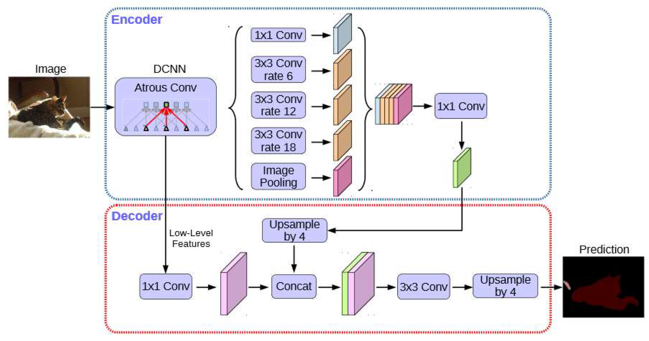
DeeplabV3+ uses the Atrous Spatial Pyramid Pooling (ASPP) mechanism which exploits the multi-scale contextual information to improve segmentation [23]. Atrous (which means holes) convolution has advantages over the standard convolution by providing responses at all image positions and while the number of filter parameters and the number of operations stay constant [23]. DeepLabV3+ has an encoder-decoder network structure. The encoder part of it consists of a set of processes that reduce the feature maps and capture semantic information and the decoder part of it recovers the spatial information and results in sharper segmentations. The block diagram of DeepLabV3+ can be seen in Figure 1.

2.1.1. Training with DeepLabV3+

A Windows 10 machine with a GPU card (RTX2070) and 16 GB memory is used for DeepLabv3+ model training and testing, which uses TensorFlow framework to run. For training a DeepLabV3+ model for any of the two datasets, the weights of a pre-trained model with the exception of the logit layer weights are used for initialization and these weights are fine-tuned with further training. These initial weights belong to a pre-trained model for the PASCAL VOC 2012 dataset (“deeplabv3_pascal_train_aug_2018_01_04.tar.gz”). Because the number of land covers in the two investigated training datasets is different from the number of classes in the PASCAL VOC-2012 dataset, the logit weights in the pre-trained model are excluded. The DeepLabV3+ training parameters used in this work can be seen in

Table 1. Training parameters used in DeepLabV3+.

Training parameter	Value
Learning policy	Poly
Base learning rate	0.0001
Learning rate decay factor	0.1
Learning rate decay step	2000
Learning power	0.9
Training number of steps	≥100,000
Momentum	0.9
Train batch size	2
Weight decay	0.00004
Train crop size	”513,513”
Last layer gradient multiplier	1
Upsample logits	True
Drop path keep prob.	1
tf_initial_checkpoint	deeplabv3_pascal_train_aug
initialize_last_layer	False
last_layers_contain_logits_only	True
slow_start_step	0
slow_start_learning_rate	1 × 10−4
fine_tune_batch_norm	False
min_scale_factor	0.5
max_scale_factor	2
scale_factor_step_size	0.25
atrous_rates	[6,12,18]
output_stride	16

. The training number of steps in DeepLabV3+ was set to 100,000 for both datasets.

2.2. Datasets Used for Training DeepLabV3+ Models

2.2.1. Slovenia Dataset

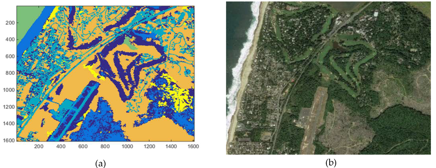
The Slovenia dataset [27] was collected by the Sentinel-2 satellite. It has a resolution of 10 m and 6 bands (L1C bands). Among these 6 bands, only the three-color image bands (RGB) are used in this investigation. In this dataset, there are originally 293 images with size of 1010 × 999. After excluding 91 images, which mostly consist of “no data” labels in their ground truth annotations, the remaining 202 images are partitioned into four non-overlapping images with size of 505 × 499. The total number of images in the modified dataset becomes 808 after this. Among these 808 images, 708 of them are randomly selected for training a DeepLabV3+ model, and 100 of them are left for testing. The eight land covers in the Slovenia dataset are: cultivated land, forest, grassland, shrub land, water, wetlands, artificial surface, and barren land. These satellite images are captured over the European country of Slovenia for the year of 2017. The Slovenia dataset contains all three vegetation types we are interested in (forest, shrub land, and grassland). An example color image from the Slovenia dataset and its ground truth annotation can be seen in Figure 2. White pixels correspond to unlabeled samples. In Figure 2b, red color is used to annotate forest, green color is used for grassland and yellow mustard color is used for shrub land annotation.

2.2.2. Oregon Dataset

The commercial company, EarthDefine, [36] provides sample land cover maps that are publicly accessible. One of these sample land cover maps containing the three vegetation types (tree, shrub and grass) is used as the second dataset in this work. Other than the tree, shrub and grass, there are three other land covers, which are bare land, impervious and water. The land cover map belongs to an area in Gleneden Beach, Oregon. The land cover map together with its reconstructed color image using the image tiles downloaded via Google Maps API [37] can be seen in Figure 3. In the land cover map, yellow color is used for shrub, dark blue color is used for grass, and orange color is used for tree annotation.

The land cover map is a single band image in geotiff format. According to the information that accompanied the sample land cover map [28], the Oregon land cover map is a high resolution (1 m) land cover data product and it is derived from 1 m, 4 band color infrared imagery flown between 5 June 2016 and 11 August 2016 as part of the National Agriculture Imagery Program (NAIP). The website also mentions that LiDAR data flown between 2009 and 2012 was used to aid the classification process [28]. Google Map API is used to retrieve corresponding the high-resolution color image tiles at an image resolution close to 25 cm for the same area of the land cover map. The procedure in [4] is used to retrieve the color image tiles from Google Maps and to reconstruct the corresponding color image. To register the reconstructed color image to the land cover map, a GDAL tool [4] is used that warps the land cover map into the same WGS84 model of the reconstructed color image. For DeepLabV3+ application, the color image and the land cover map are partitioned into 404 image patches of size 512 × 512. All these 404 image tiles contain at least one type of vegetation type or more. Among these 404 image patches, 304 of them are randomly selected for training and 100 of them are randomly selected for testing. Because the land cover map has a data collection time of 2016 and the color image data collection time is 2019, it is likely that there could be some discrepancies between the land cover map and the color image.

3. Vegetation Classification Results

3.1. Forest-Grassland-Shrub Classification in Slovenia Dataset with Eight Classes

In this investigation, all eight land covers in Slovenia dataset are used, of which three of the land covers are forest (tree), shrub land (shrub), and grassland (grass). Two DeepLabV3+ models are trained for two cases: (a) Uniform weights for the 8 classes in model training, (b) median frequency weights for the 8 classes.

The number of pixels for each land cover, which is denoted by “pixel count,” its frequency and the median frequency balancing weights for the Slovenia dataset can be seen in

Table 2. Pixel numbers for each class and the computed median frequency class weights used in DeepLabV3+ training (Slovenia 8-class).

	Cultivated Land	Forest	Grassland	Shrub Land	Water	Wetlands	Artificial Surface	Bare Land
Pixel Count	22,027,446	1.14 × 108	35,172,713	7,186,382	1,285,398	115,238	10,689,454	1,189,780
Frequency	0.1192	0.5942	0.1838	0.0375	0.0070	0.0022	0.0558	0.0242
Weights	0.3918	0.0786	0.2541	1.2437	6.6455	21.4237	0.8361	1.9334

. To provide a physical sense of pixel count values to area, it is worth mentioning that 10,000 pixels correspond to an area of 1 km² in the Slovenia dataset. In Table 2, the term frequency represents the number of pixels of the class divided by the total number of pixels in images that had an instance of that class [30]. The median frequency balancing weight of class C is then computed by median frequency divided by the frequency of class C [30]. In Table 2, the median frequency balancing weights are denoted by the “weights” row. From Table 2, it can be noticed that the number of pixels for some of the classes such as Wetlands and Water and their corresponding frequency are quite low in number. A significant imbalance can be seen between shrub land and other vegetation classes (grassland and forest). After median frequency weighting, the Water and Wetlands have heavier weighting.

The confusion matrix for the uniform weights and median frequency weight cases can be seen in

Table 3. Confusion matrix with uniform weights (Slovenia—8 classes).

	Cultivated Land	Forest	Grassland	Shrub Land	Water	Wetlands	Artificial Surface	Bare Land
Cultivated Land	1,807,364	90,850	931,365	5676	5207	0	117,708	0
Forest	30,394	12,821,508	299,710	29,455	13,244	0	31,234	864
Grassland	614,857	512,343	3,304,042	26,335	9551	0	181,282	1585
Shrub land	57,773	402,058	280,887	85,051	10,690	0	39,455	24,269
Water	13,113	30,500	28,924	3476	76,374	0	15,258	0
Wetlands	162	3443	4086	189	139	0	267	0
Artificial Surface	119,005	143,645	345,149	7845	10,636	0	761,973	1
Bare land	13	12,678	4968	20,947	268	0	573	35,527

and

Table 4. Confusion matrix with median frequency class weights (Slovenia—8 classes).

	Cultivated Land	Forest	Grassland	Shrub Land	Water	Wetlands	Artificial Surface	Bare Land
Cultivated Land	1,953,238	19,478	487,144	149,709	61,131	2282	285,188	0
Forest	93,435	10,808,853	349,884	1,593,515	229,474	18,139	126,762	6347
Grassland	933,246	196,031	2,210,529	608,756	158,336	12,963	524,870	5264
Shrub land	61,029	122,016	109,380	430,463	65,617	3692	71,298	36,688
Water	9122	3667	6399	6840	131,225	561	9831	0
Wetlands	543	1298	2072	2211	774	611	777	0
Artificial Surface	122,403	52,069	140,862	95,020	89,631	3188	885,050	31
Bare land	0	1846	2113	25,618	1513	0	223	43,661

, respectively. The class accuracy for each land cover, averaged class accuracy for eight classes, averaged class accuracy for three vegetation classes, overall accuracy and the kappa metric values [38] can be seen in

Table 5. Accuracy (uniform and median weights, Slovenia—8 classes).

	Cultivated Land	Forest	Grass Land	Shrub Land	Water	Wet Lands	Artificial Surface	Bare Land	Average (8classes)	Average (3vegcls)	Overall Accuracy	Kappa
Uniform	0.6110	0.9694	0.7105	0.0945	0.4556	0.0000	0.5489	0.4739	0.4830	0.5915	0.8082	0.6798
Median	0.6603	0.8172	0.4754	0.4782	0.7828	0.0737	0.6375	0.5823	0.5634	0.5903	0.7044	0.5610

. Intersection over union (IoU) values for each land cover and mean IoU (mIoU) can be seen in

Table 6. Intersection over union (IoU) (uniform and median weights, Slovenia—8 classes).

	Cultivated Land	Forest	Grass Land	Shrub Land	Water	Wetlands	Artificial Surface	Bare Land	mIoU
IoU (Uniform)	0.4764	0.8890	0.5048	0.0856	0.3513	0.0000	0.4295	0.3494	0.3858
IoU (Median)	0.4675	0.7934	0.3846	0.1273	0.1695	0.0124	0.3677	0.4675	0.3346

. IoU is defined as the intersection area over the union of the area [39]. With respect to the three vegetation classifications, using uniform weights, shrub land classification accuracy is extremely poor with a value of 0.0945 and from the confusion matrix in Table 3, it is noticed that the shrub land pixels are misclassified mostly as forest or grassland. This observation indicates the challenges using only RGB color images especially when the training data is heavily imbalanced. In many classifiers including the deep learning ones when the dataset is heavily imbalanced, the error from the overrepresented classes contributes much more to the loss value than the error contribution from the underrepresented classes. This makes the deep learning method’s loss function to be biased toward the overrepresented classes resulting in poor classification performance for the underrepresented classes such as shrub in this case.

With the use of median frequency weights when training a DeepLabV3+ model, the shrub land class accuracy increased significantly from 0.0945 to 0.4782 and the average eight-class accuracy also increased considerably from 0.4830 to 0.5634. The overall accuracy (eight classes) is found to be 0.8082 with uniform weights and was reduced to 0.7044 with median frequency weights. The decrease in the overall accuracy with median frequency weights is understandable since even though using median frequency weights helps to improve the classification accuracy of underrepresented classes, the trade-off comes as a reduction in the classification accuracy values of the overrepresented classes which then results in the reduction in overall accuracy. With respect to kappa and mIoU measures, both have lower values when median frequency weights are used. Even though the average accuracy for the eight classes is significantly improved, with respect to the three vegetation classes, the average accuracy stayed the same with median frequency weights in comparison to uniform weights.

3.2. Forest-Grassland-Shrub Classification in Slovenia Dataset with Three Vegetation Classes

The same investigation is applied by including only the three vegetation classes (forest, shrub, and grass) and excluding all other land cover types from the classification. This investigation assumes that the three vegetation classes can be separated from other land covers. The objective of this investigation was to create a pure classification scenario that includes the three vegetation classes only to eliminate the impact of all other land covers’ misclassifications on the three vegetation classes’ accuracy. Similarly, two DeepLabV3+ models are trained with uniform and median frequency weights. All other non-vegetation classes (cultivated land, water, wetlands, artificial surface, and bare land) are excluded by labeling them as ignore during training of DeepLabV3+ models. The pixel counts for each of the three vegetation classes, class frequency, and the median frequency balancing weights for the three classes can be seen in

Table 7. Pixel numbers for the three classes, class frequency and median frequency class weights used in DeepLabV3+ training (Slovenia—3 classes).

	Forest	Grassland	Shrub Land
Pixel Count	1.14 × 108	35,172,713	7,186,382
Frequency	0.7286	0.2253	0.0460
Weights	0.3093	1.0000	4.8944

. It can be noticed that forest has the highest pixel count followed by grassland. The shrub land has the lowest number of pixels among the three vegetation classes.

Table 8. Confusion matrices for uniform and median frequency class weights (Slovenia—3 classes).

	Uniform Weights			Median Frequency Class Weights
	Forest	Grassland	Shrub Land	Forest	Grassland	Shrub Land
Forest	12,854,713	321,868	49,828	11,276,673	305,569	1,644,167
Grassland	512,527	4,087,228	50,240	134,329	3,703,555	812,111
Shrub land	409,089	347,316	143,778	111,943	165,749	622,491

,

Table 9. Accuracy (uniform and median weights, Slovenia—3 classes).

	Forest	Grassland	Shrub Land	Average	Overall Accuracy	Kappa
Uniform weights	0.9719	0.8790	0.1597	0.6702	0.9099	0.7855
Median weights	0.8526	0.7965	0.6915	0.7802	0.8310	0.6651

and

Table 10. IoU (uniform and median weights, Slovenia—3 classes).

	Forest	Grassland	Shrub Land	mIoU
Uniform weights	0.9086	0.7684	0.1437	0.6069
Median weights	0.8370	0.7232	0.1855	0.5819

correspond to the confusion matrix, accuracy, and IoU-related measures for the three vegetation-class-only results with uniform and median frequency weights. It can be noticed from Table 9 that with median frequency weights, the correct classification accuracy of shrub land, which was very poor with uniform weights, significantly improved from 0.1597 to 0.6915. When uniform weights are used, most of the shrub land pixels were mostly misclassified as forest according to the confusion matrix. The average classification accuracies also improved from 0.6702 to 0.7802 with median frequency weights. The overall accuracy values were reduced from 0.9099 to 0.8310 since forest and grassland accuracy values dropped with the use of median frequency weights as a trade-off to the significant accuracy improvement in shrub land classification. Similar patterns are observed with the IoU measure.

Table 11. Vegetation class accuracy comparisons for three and eight class models in DeepLabV3+.

	Forest	Grassland	Shrub Land	Average Accuracy
Uniform, (Slovenia—8 classes)	0.9694	0.7105	0.0945	0.5915
Uniform, (Slovenia—3 veg. classes only)	0.9719	0.8790	0.1597	0.6702
Median, (Slovenia—8 classes)	0.8172	0.4754	0.4782	0.5903
Median, (Slovenia—3 veg. classes only)	0.8526	0.7965	0.6915	0.7802

shows the three vegetation classification accuracy comparisons with three and eight class DeepLabV3+ models. From Table 11, it can be noticed that classification accuracies for all three vegetation types (forest, grass, and shrub) improve with the three-vegetation-class classification only in comparison to including all land covers in an 8-class classification. Even though using median frequency weights results in some reduction in the classification accuracies of forest and grassland, in return, the classification accuracy of shrub land gets a significant boost. From Table 11, it can be also noticed that among the three vegetation classes, shrub land has the lowest correct classification accuracy whereas forest has the highest. This finding about the classification difficulty ranking of these three vegetation types makes sense from a visual perspective, since among them forest and grass land have more easily distinguishable spatial features relative to shrub and form the two opposite sides of the visualization range and shrub stays somewhere between forest and grass land in this range. The confusion matrices support this by revealing that shrub land is misclassified as tree or grass by large amounts whereas the misclassification ratio is smallest in forest followed by grass land.

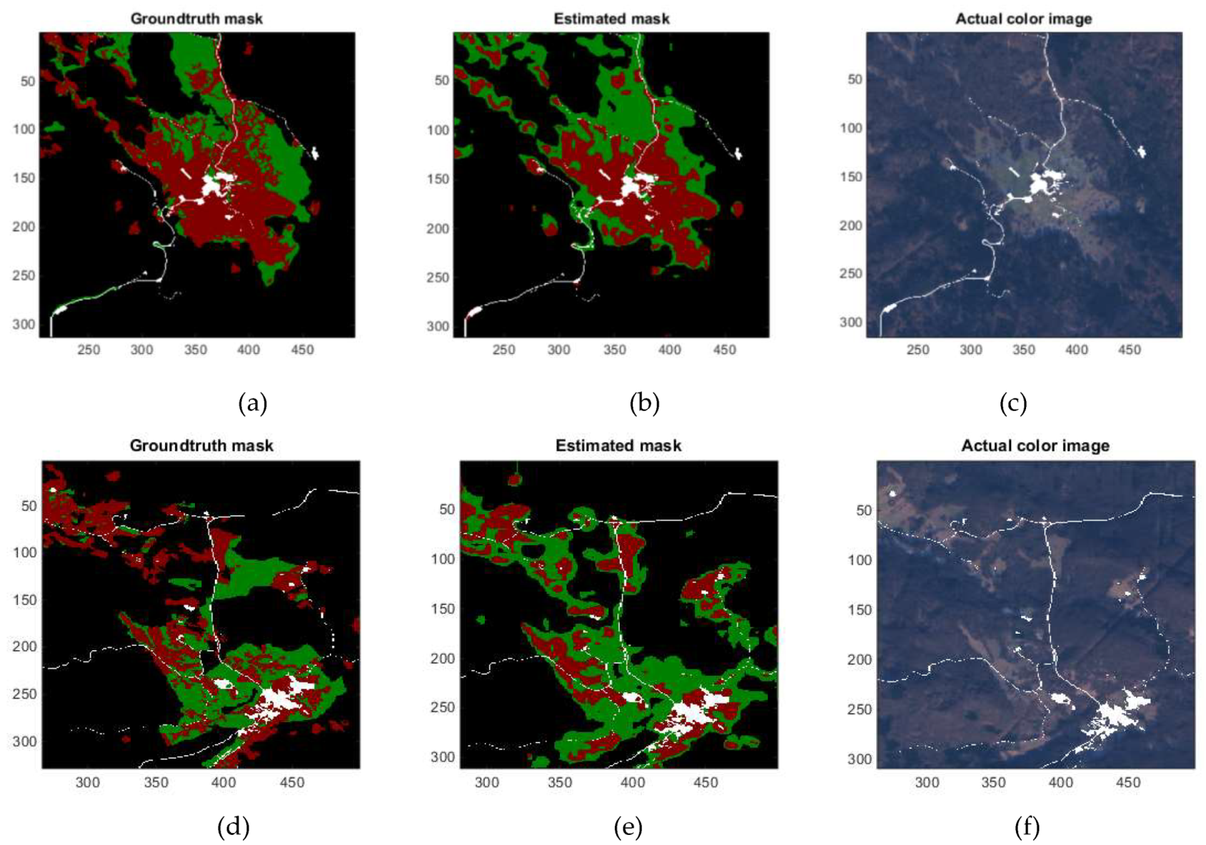
We provided screenshots of two images in the Slovenia test dataset (three-vegetation class DeepLabv3+ model trained using median frequency weights). We included the color images together with the estimated and ground truth land cover maps. In the land cover maps in Figure 4, black color corresponds to forest, red color corresponds to grassland, green color corresponds to shrub land, and white color corresponds to ignore class which corresponds to the pixel locations that are excluded from DeepLabV3+ model training. Even though color images look very challenging for classification due to low resolution, DeepLabV3+ is found to perform considerably well.

3.3. Tree-Grass-Shrub Classification in Oregon Dataset with Six Land Cover Types

In this investigation, all six land covers of Oregon dataset are used in the classification, three of which are tree, grass, and shrub.

Table 12. Pixel numbers for each class and the computed median frequency class weights used in DeepLabV3+ training (Oregon—6 classes).

	Tree	Shrub	Grass	Bare	Impervious	Water
Pixel Count	40,196,934	3,531,951	21,257,350	10,390,934	16,691,487	350,309
Frequency	0.4777	0.0666	0.2376	0.1309	0.2636	0.1114
Weights	0.3857	2.7669	0.7755	1.4076	0.6991	1.6543

shows the pixel counts for each land cover and the corresponding median frequency weight values used for DeepLabv3+ model training. Considering the ~25 cm image resolution, an area of 1 km² corresponds to about 16 million pixels in the Oregon dataset.

Table 13. Confusion matrix with uniform weights (Oregon—6 classes).

	Tree	Shrub	Grass	Bare	Impervious	Water
Tree	10,176,979	26,739	420,678	14,881	390,883	0
Shrub	278,319	500,512	194,788	6451	30,835	0
Grass	642,276	163,119	4,043,947	298,527	237,164	711
Bare	36,687	12,655	393,307	1,502,801	42,893	0
Impervious	529,003	2173	154,265	18,337	2,821,653	0
Water	6340	0	40,766	3020	0	66,076

and

Table 14. Confusion matrix (with median frequency class weights, Oregon—6 classes).

	Tree	Shrub	Grass	Bare	Impervious	Water
Tree	9,716,493	41,448	617,935	37,610	615,087	1587
Shrub	208,148	634,776	135,480	9258	23,243	0
Grass	513,603	215,910	3,957,360	423,519	267,767	7585
Bare	25,499	20,973	259,716	1,641,949	40,206	0
Impervious	414,228	18,684	188,444	20,350	2,883,725	0
Water	5014	0	26,883	0	0	84,305

correspond to the resultant confusion matrices with uniform and median frequency weights, respectively.

Table 15. Accuracy (uniform and median weights, Oregon—6 classes).

	Tree	Shrub	Grass	Bare	Imp.	Water	Average (6 Classes)	Average (3 veg Classes)	Overall Accuracy	Kappa (6 Classes)
Uniform	0.9227	0.4951	0.7509	0.7558	0.8004	0.5686	0.7156	0.7229	0.8289	0.7458
Median	0.8809	0.6279	0.7348	0.8258	0.8180	0.7255	0.7688	0.7479	0.8205	0.7386

and

Table 16. IoU (uniform and median weights, Oregon—6 classes).

	Tree	Shrub	Grass	Bare	Imp.	Water	mIoU
IoU (uniform weights)	0.8127	0.4117	0.6137	0.6451	0.6675	0.5652	0.6193
IoU (median weights)	0.7967	0.4853	0.5983	0.6623	0.6449	0.6724	0.6433

show the accuracy-and IoU-related measures. With the use of median frequency weights, the shrub classification accuracy increased significantly from 0.4951 to 0.6279 and the average classification accuracy increased from 0.7156 to 0.7688. Similar trends that were observed in the Slovenia dataset with respect to shrub and average classification accuracy were also observed in this dataset. Different from Slovenia dataset results, there are almost no changes in the overall accuracy and kappa values when switching from uniform weights to median frequency weights. An increase in mIoU value is also observed with median frequency weights.

3.4. Tree-Grass-Shrub Classification in Oregon Dataset with Three Land Cover Types

Only the three vegetation classes (tree, shrub, and grass) are included in the classification.

Table 17. Pixel numbers for the three classes, class frequency and median frequency class weights used in DeepLabV3+ training (Oregon—3 class).

	Tree	Shrub	Grass
Pixel Count	40,202,025	3,533,766	21,267,871
Frequency	0.6612	0.1018	0.3427
Weights	0.5183	3.3657	1.000

shows the pixel counts for the three vegetation classes and median frequency weights

Table 18. Confusion matrices for uniform and median frequency class weights (Oregon—3 classes).

	Uniform Weights			Median Frequency Class Weights
	Tree	Shrub	Grass	Tree	Shrub	Grass
Tree	10,505,813	31,198	494,456	10,241,835	62,228	727,404
Shrub	288,384	551,809	171,122	260,426	598,451	152,438
Grass	807,860	153,182	4,427,040	603,966	220,577	4,563,539

,

Table 19. Accuracy (uniform and median weights) and Kappa values (Oregon—3 classes).

	Tree	Shrub	Grass	Average (3 Classes)	Overall Accuracy	Kappa
Uniform weights	0.9523	0.5456	0.8216	0.7732	0.8883	0.7703
Median weights	0.9284	0.5918	0.8470	0.7890	0.8837	0.7662

and

Table 20. IoU and mean IoU (mIoU) values (uniform and median weights, Oregon—3 classes).

	Tree	Shrub	Grass	mIoU
Uniform weights	0.8663	0.4615	0.7313	0.6864
Median weights	0.8610	0.4624	0.7281	0.6838

correspond to the confusion matrices, accuracy-, and IoU-related measures with uniform and median frequency weights. Here, tree is the overrepresented class and shrub is the underrepresented class. It is worth mentioning that relatively there are more shrub pixels in the Oregon dataset in comparison to Slovenia dataset. With median frequency weights, considerable improvements can be seen mainly in shrub classification accuracy, increasing from 0.5456 to 0.5918, followed by an improvement in grass classification accuracy, from 0.8216 to 0.8470. Tree classification accuracy, however, drops from 0.9523 to 0.9284 as was expected since it is the overrepresented class. Overall, the average classification accuracy improves by about 1.6%, from 0.7732 to 0.7890. The improvement in average classification accuracy after switching to median frequency weights is not as significant as the improvement that was observed in the Slovenia dataset, since there are relatively more shrub pixels in the Oregon dataset and since Oregon dataset is a higher resolution dataset relatively better classifications for shrub are observed with uniform weights in comparison to the Slovenia dataset where shrub is severely underrepresented.

Table 21. Vegetation class accuracy for six and three-class models in DeepLabV3+.

	Tree	Grass	Shrub	Average Accuracy
Uniform, (Oregon—6 classes)	0.9227	0.7509	0.4951	0.7229
Uniform, (Oregon—3 veg. classes only)	0.9523	0.8216	0.5456	0.7732
Median, (Oregon—6 classes)	0.8809	0.7348	0.6279	0.7479
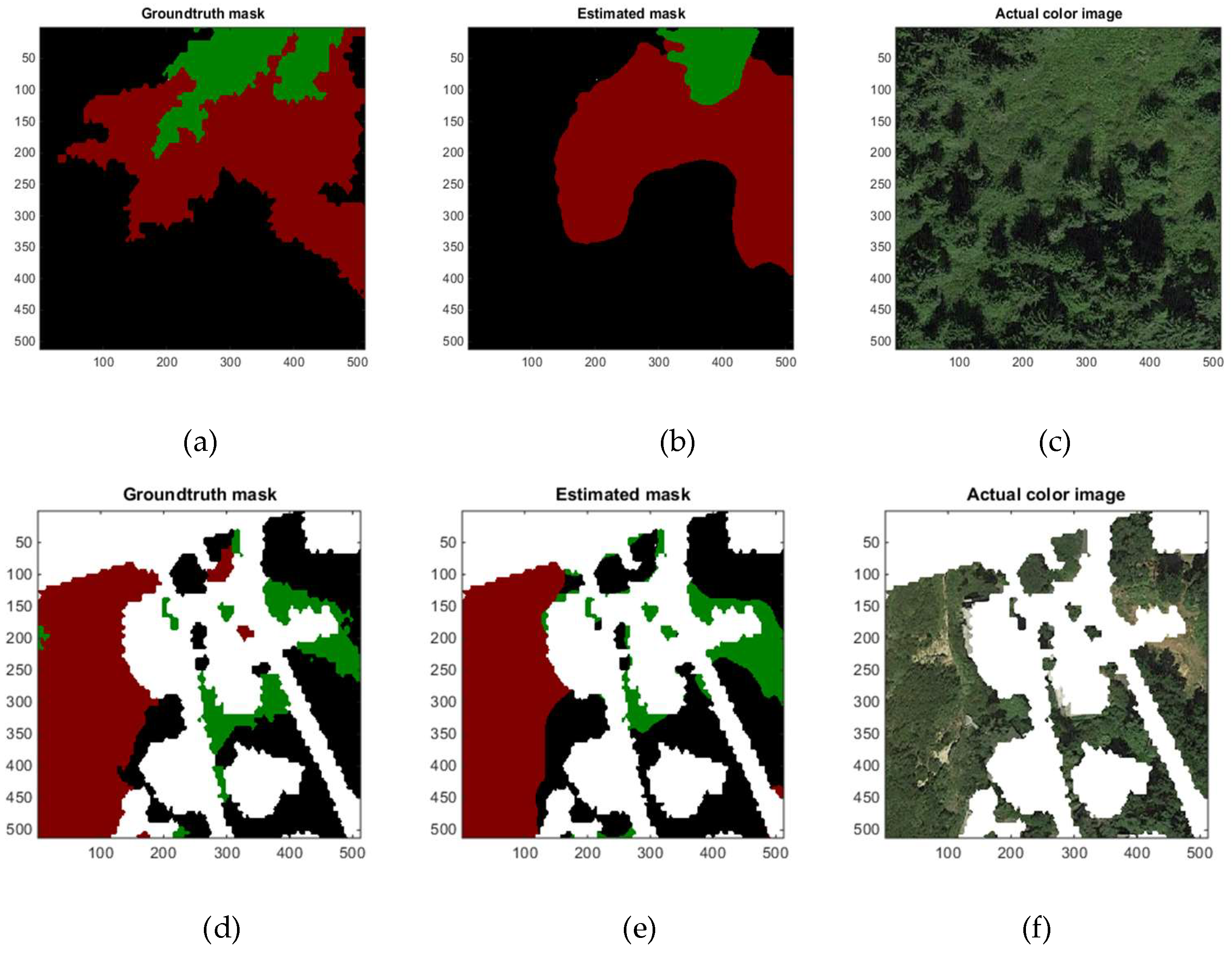
Median, (Oregon—3 veg. classes only)	0.9284	0.8470	0.5918	0.7890

shows the three vegetation classification accuracy comparisons with both three and six class models in DeepLabV3+. From Table 21, it can be seen that classification accuracies for all three vegetation types (tree, grass, and shrub) improve with the three-vegetation-only classification in comparison to including all land covers. The only exception was shrub with median frequency weights. Even though using median frequency weights results in some reduction in the classification accuracies of tree, in return, the classification accuracy of shrub and grass improves. Similar to the Slovenia dataset, among the three vegetation classes, shrub is found to have the lowest correct classification accuracy whereas tree has the highest correct classification accuracy. Sample screenshots from two image samples of Oregon test dataset (three-vegetation class DeepLabv3+ model trained using median frequency weights) can be seen in Figure 5.

3.5. Sampled Pixels Investigation for Comparison of DeepLabv3+ with Pixel-Based Classifiers

The classification performance and computation time comparison of DeepLabV3+ with two pixel-based classification methods are conducted on sampled pixel sets from the three vegetation classes. These two classifiers are support vector machine (SVM) [31] and random forest (RF) [32]. The features used with the two classifiers are the RGB values (for baseline), GLCM, and Gabor texture features extracted from batch images of size 21 × 21, and a combined set of GLCM and Gabor texture features. This investigation is to assess DeepLabV3+’s performance with respect to two well-known pixel-based classification methods. Both Slovenia and Oregon datasets are used in the investigation.

Using the ground truth land cover maps, separate maps for each of the three vegetation types are generated. An erosion morphology operator is applied to these maps with a square structuring element of size 21. From each of the eroded individual land cover maps of the training data set, ~100,000 pixels for each vegetation type (~300,000 total) are randomly selected from the Slovenia dataset. Using these pixel locations, the batch images of size 21 × 21 are identified where the selected pixel is in the center of the identified batch image. This process enabled selecting homogeneous land cover pixels for the three vegetation types which can then be used for training the pixel-based classifier models. By using equal number of pixels from each vegetation type when forming training data, it is aimed to exclude the data imbalance effects from the classification analyses. In addition to training separate models using GLCM features, Gabor features and combined GLCM/Gabor texture features, we also trained SVM and RG models using RGB values of the selected pixels for baseline.

GLCM texture features (total of 17 features) and Gabor textures features (total of 28 features) are extracted from the batch images for the ~300,000 pixels locations [5]. Using these extracted training features, ~100,000 for each vegetation type (~300,000 total), SVM and RF models are trained for Slovenia and Oregon datasets separately. Regarding test data, we randomly selected ~26,000 pixel locations from each of the three vegetation types (~78,000 total) to form the test data in Slovenia dataset. We randomly picked 400,000 pixel locations from each of the three vegetation types (1,200,000 total) to form the test data in Oregon dataset. We needed to use less number of pixels in the Slovenia test data since there were not that many homogenous shrub image patches in the Slovenia test data.

For SVM we used LibSVM tool [40] with C-SVM classification with the RBF (radial basis function) kernel. For optimal SVM parameters (g and c), LibSVM’s parameter selection tool is used. This tool uses cross validation (CV) technique to estimate the accuracy of each parameter combination in the specified range. When using this tool, five-fold cross validation is applied. For c parameter, we scanned the a range of c as: c_range = 2^{-5,-3,-1,1,3,5,7,9,11,13,15} and for g parameter, we scanned a range of g as: g_range = 2^{3,1,-1,-3,-5,-7,-9,-11,-13,-15}. For RF, we used the Matlab source codes in [41]. We set the number of trees, ntree, to 500 after trial and error to find the highest classification and let the other RF parameter, mtry, to be automatically identified based on the total number of features. For technical information about RF and its parameters (ntree and mtry), one can refer to [41].

Table 22. Accuracy and kappa values for sampled pixels investigation in Slovenia dataset.

	Accuracy (Forest)	Accuracy (Grassland)	Accuracy (Shrub Land)	Average Accuracy	Kappa
DeepLabv3+ (median weights)	0.9610	0.9297	0.8770	0.9226	0.8839
SVM (RGB) (c = 2048, g = 2)	0.8538	0.8246	0.6161	0.7648	0.6474
SVM (GLCM) (c = 32, g = 2)	0.8994	0.7981	0.6151	0.7709	0.6564
SVM (Gabor) (c = 8, g = 2)	0.9684	0.0945	0.7244	0.5958	0.3935
SVM (GLCM/Gabor) (c = 32, g = 2)	0.9409	0.5609	0.6448	0.7155	0.5733
Random Forest (RGB) (ntree = 500, mtry = 1)	0.8154	0.8133	0.6569	0.7618	0.6428
Random Forest (GLCM) (ntree = 500, mtry = 4)	0.8800	0.7706	0.6521	0.7675	0.6513
Random Forest (Gabor) (ntree = 500, mtry = 5)	0.9904	0.0604	0.6393	0.5634	0.3449
Random Forest (GLCM/Gabor) (ntree = 500, mtry = 6)	0.9622	0.6576	0.6429	0.7542	0.6314

shows the three vegetation class accuracies, average classification accuracy and kappa values for DeepLabV3+, and the two pixel-based classifiers for the Slovenia dataset. The two pixel-based classifiers use RGB pixel values (for baseline), GLCM features, Gabor features and combined GLCM/Gabor features. For DeepLabV3+, the segmentation estimations of DeepLabV3+ for the randomly selected pixel locations are simply retrieved from the previously generated results with median frequency weights and used in generating the performance measures.

Table 23. IoU and mIoU values for sampled pixels investigation in Slovenia dataset.

	IoU (Forest)	IoU (Grassland)	IoU (Shrub Land)	mIoU
DeepLabv3+ (median weights)	0.8811	0.8887	0.8006	0.8568
SVM(RGB) (c = 2048, g = 2)	0.6512	0.7022	0.5051	0.6195
SVM(GLCM) (c = 32, g = 2)	0.6404	0.6905	0.5459	0.6256
SVM(Gabor) (c = 8, g = 2)	0.4854	0.0919	0.6090	0.3954
SVM(GLCM/Gabor) (c = 32, g = 2)	0.5699	0.5233	0.5705	0.5545
Random Forest (RGB) (ntree = 500, mtry = 4)	0.6392	0.6995	0.5148	0.6178
Random Forest (GLCM) (ntree = 500, mtry = 4)	0.6243	0.6832	0.5621	0.6232
Random Forest (Gabor) (ntree = 500, mtry = 5)	0.4559	0.0600	0.5649	0.3603
Random Forest (GLCM/Gabor) (ntree = 500, mtry = 6)	0.6103	0.6238	0.5811	0.6051

shows the IoU measures for each of the three vegetation class and mIoU. Similarly

Table 24. Accuracy and kappa values for sampled pixels investigation in Oregon dataset.

	Accuracy (Tree)	Accuracy (Grass)	Accuracy (Shrub)	Average Accuracy	Kappa
DeepLabv3+ (median weights)	0.9629	0.9111	0.7157	0.8632	0.7948
SVM(RGB) (c = 2048, g = 8)	0.7632	0.4520	0.7210	0.6364	0.4546
SVM (GLCM) (c = 512, g = 2)	0.8076	0.6814	0.7670	0.7520	0.6280
SVM (Gabor) (c = 8, g = 2)	0.9067	0.7523	0.4036	0.6875	0.5313
SVM (GLCM/Gabor) (c = 8, g = 0.5)	0.9337	0.8686	0.6939	0.8321	0.7481
Random Forest (RGB) (ntree = 500, mtry = 1)	0.7394	0.5136	0.6758	0.6430	0.4644
Random Forest (GLCM) (ntree = 500, mtry = 4)	0.8165	0.7140	0.7364	0.7556	0.6334
Random Forest (Gabor) (ntree = 500, mtry = 5)	0.9416	0.7147	0.3472	0.6678	0.5018
Random Forest (GLCM/Gabor) (ntree = 500, mtry = 6)	0.9242	0.8486	0.7151	0.8293	0.7440

and

Table 25. IoU and mIoU values for sampled pixels investigation in Oregon dataset.

	IoU (Tree)	IoU (Grass)	IoU (Shrub)	mIoU
DeepLabv3+ (median weights)	0.7480	0.8400	0.6892	0.7591
SVM(RGB) (c = 2048, g = 8)	0.5481	0.4001	0.4456	0.4646
SVM(GLCM) (c = 512, g = 2)	0.6246	0.6520	0.5455	0.6074
SVM(Gabor) (c = 8, g = 2)	0.5577	0.6143	0.3713	0.5145
SVM(GLCM/Gabor) (c = 8, g = 0.5)	0.7045	0.8252	0.6163	0.7153
Random Forest (RGB) (ntree = 500, mtry = 1)	0.5471	0.4336	0.4403	0.4737
Random Forest (GLCM) (ntree = 500, mtry = 4)	0.6240	0.6618	0.5472	0.6110
Random Forest (Gabor) (ntree = 500, mtry = 5)	0.5350	0.6252	0.3176	0.4926
Random Forest (GLCM/Gabor) (ntree = 500, mtry = 6)	0.7013	0.8217	0.6156	0.7129

correspond to the accuracy and IoU-related measures for the Oregon dataset. From the results, it can be seen that in both datasets DeepLabV3+ performs significantly better than the two pixel-based classifiers.

Table 26. Approximate computation times of the three classification methods for three-class Slovenia dataset.

	Data	Training	Testing	Comments
DeepLabv3+ (median weights)	All pixels in 808 images each with size 499 × 505 (178,412,460 pixels for 708 training images and 25,199,500 test image pixels)	15 h 22 mins 40 s (100,000 epoch training of 708 images with size 499 × 505)	36 s (for 100 test images of size 499 × 505)	DeepLabv3′s pascal model is used as the initial checkpoint in training. RTX2070 GPU is used.
SVM (GLCM, 17 features, c = 32, g = 2)	Sampled pixels (300,000 training pixels and 78,107 test pixels for three vegetation classes) from 808 images	1 h 14 min 55 s	2 min 5 secs	PC with Intel i7-9700K CPU, 16GB RAM, and Win10 operating system
Random Forest (GLCM, 17 features, ntrees = 500, mtry = 4)	Sampled pixels (300,000 training pixels and 78,107 test pixels for three vegetation classes) from 808 images	10 min 21 secs	4.58 sec	PC with Intel i7-9700K CPU, 16GB RAM, and Win10 operating system

shows the comparison of DeepLabV3+ with these two classifiers with respect to computation time (model training and testing). Slovenia dataset is used for computation time comparison and GLCM features (total 17 features) are used in the two pixel-based classifiers. It can be seen that DeepLabV3+ has the longest model training time but its test time is less than SVM. RF is the fastest method both in training and testing times while providing classification accuracy close to SVM. Overall, the results showed that DeepLabV3+ provides more accurate classification results than these two pixel-based classifiers with a trade-off for a longer model training time.

3.6. Discusssion

Even though height data in the form of DTM could add significant capability to classify the three similar looking vegetation land covers (tree, shrub, and grass), obtaining height data via LiDAR could be costly and DTM estimates from LiDAR for lower heights may also not be highly accurate. DTM estimation via stereo images could be an alternative to LiDAR but this also has its own challenges in terms of noisy DTM estimations especially at lower heights. The use of NIR band helps detecting vegetation when used with Red band via NDVI index but faces setbacks when it comes to classifying vegetation land covers with similar spectral characteristics such as tree, shrub, and grass. As an example, in [3], together with Red, Green, NIR band images, LiDAR were also used for land cover classification and different from our work, the authors combined trees and shrubs into a single class which is relatively a less challenging problem than ours since in our case tree, shrub, and grass are set as three separate classes. In [3], it is reported that if only RG and NIR data were used, the classification accuracy of “trees and shrubs” was only 52.9%. With LiDAR, the authors stated that the classification performance was improved to 89.7%. We achieved ~59.0% average classification accuracy for the three vegetation classes in the 8-class case and 78.0% for the three-class vegetation-only case in the low-resolution Slovenia dataset. In the high-resolution Oregon dataset, we achieved ~74.8% average classification accuracy for the three vegetation classes in the 6-class case and ~78.9% for the three-class vegetation-only case. Considering that only RGB color bands were used without LiDAR or NIR bands and that each of these three vegetation types has its own class, the classification results with DeepLabV3+ using median frequency weights are found quite remarkable.

4. Conclusions

Without using NIR and LiDAR, it is challenging to correctly classify trees, shrubs, and grass. In some cases, even the use of NIR and LiDAR may not provide highly accurate results and it is important to utilize auxiliary methods which could be used as supportive information to increase the confidence of the classification decisions using LiDAR data. In this paper, we report some new results using a semantic segmentation based deep learning method to tackle the above challenging problem using only RGB images.

We provided a comprehensive evaluation of DeepLabV3+ for classification of three similar looking vegetation types, which are tree, shrub, and grass, using color images only with both low resolution and high resolution datasets. The data imbalance issue with DeepLabV3+ is discussed and it is demonstrated that the average class accuracy can be increased considerably in DeepLabV3+ using median frequency weights during model training in contrast to using uniform weights. It is observed from both datasets that higher tree, grass, and shrub classification accuracy can be achieved with DeepLabV3+ if the classification can be limited to these three vegetation classes only rather than including all other land cover types that are present in the color image datasets. In both Slovenia and Oregon datasets, it is observed that the highest classification accuracy corresponds to “tree” type whereas “shrub” type is found the most challenging to classify accurately. In addition, the performance of DeepLabV3+ is compared with two state-of-the-art machine learning classification algorithms (SVM and random forests) which use RGB pixel values, GLCM and Gabor texture features, and combination of the two sets of texture features. It is observed that DeepLabV3+ outperforms both SVM and random forests. Being a semantic segmentation-based method, DeepLabV3+ has advantages over pixel-based classifiers by utilizing both spectral (via RGB bands only) and spatial information.

Future research directions include customization of DeepLabV3+ framework to accept more than three channels (adding NIR band to three color bands) and utilization of digital terrain model (DTM) in the form of using LiDAR sensor data or in the form estimating DTM through stereo satellite images to further improve the classification accuracy of tree, grass, and shrub.

References

- Tan, K.; Zhang, Y.; Wang, X.; Chen, Y. Object-based change detection using multiple classifiers and multi-scale uncertainty analysis. Remote Sens. 2019, 11, 359. [Google Scholar] [CrossRef] [Green Version]
- Skarlatos, D.; Vlachos, M. Vegetation removal from UAV derived DSMS, using combination of RGB and NIR imagery. In Proceedings of the ISPRS Annals of Photogrammetry, Remote Sensing and Spatial Information Sciences, Riva del Garda, Italy, 4–7 June 2018; Volume IV-2, pp. 255–262. [Google Scholar]
- Hellesen, T.; Matikainen, L. An object-based approach for mapping shrub and tree cover on grassland habitats by use of LiDAR and CIR orthoimages. Remote Sens. 2013, 5, 558–583. [Google Scholar] [CrossRef] [Green Version]
- Gonçalves-Seco, L.; Miranda, D.; Crecente, R.; Farto, J. Digital terrain model generation using airborne LiDAR in a forested area Galicia, Spain. In Proceedings of the 7th International Symposium on Spatial Accuracy Assessment in Natural Resources and Environmental Sciences, Lisbon, Portugal, 5–7 July 2006. [Google Scholar]
- Ayhan, B.; Kwan, C. A Comparative Study of Two Approaches for UAV Emergency Landing Site Surface Type Estimation. In Proceedings of the 44th Annual Conference of the IEEE Industrial Electronics Society, Washington, DC, USA, 21–23 October 2018. [Google Scholar]
- Ayhan, B.; Kwan, C.; Budavari, B.; Larkin, J.; Gribben, D. Semi-automated emergency landing site selection approach for UAVs. IEEE Trans. Aerospace Electron. Syst. 2019, 55, 1892–1906. [Google Scholar] [CrossRef]
- Guirado, E.; Tabik, S.; Alcaraz-Segura, D.; Cabello, J.; Herrera, F. Deep-learning versus OBIA for scattered shrub detection with Google earth imagery: Ziziphus Lotus as case study. Remote Sens. 2017, 9, 1220. [Google Scholar] [CrossRef] [Green Version]
- Lindgren, D. Land Use Planning and Remote Sensing; Taylor & Francis: Milton, UK, 1984; Volume 2. [Google Scholar]
- Yang, L.; Wu, X.; Praun, E.; Ma, X. Tree detection from aerial imagery. In Proceedings of the 17th ACM SIGSPATIAL International Conference on Advances in Geographic Information Systems, Seattle, DC, USA, 3–6 November 2009; pp. 131–137. [Google Scholar]
- Riano, D.; Chuvieco, E.; Ustin, S.L.; Salas, J.; Rodríguez-Perez, J.R.; Ribeiro, L.M.; Fernandez, H. Estimation of shrub height for fuel-type mapping combining airborne LiDAR and simultaneous color infrared ortho imaging. Int. J. Wildland Fire 2007, 16, 341–348. [Google Scholar] [CrossRef] [Green Version]
- The Ames Stereo Pipeline, NASA’s Open Source Automated Stereogrammetry Software, Version 2.6.2. Available online: https://github.com/NeoGeographyToolkit/StereoPipeline/releases/download/v2.6.2/asp_book.pdf (accessed on 1 April 2020).
- De Franchis, C.; Meinhardt-Llopis, E.; Michel, J.; Morel, J.M.; Facciolo, G. An automatic and modular stereo pipeline for pushbroom images. In Proceedings of the ISPRS Annals of the Photogrammetry, Remote Sensing and Spatial Information Sciences, Zurich, Switzerland, 18–20 September 2014; Volume II, pp. 49–56. [Google Scholar]
- Qin, R. RPC stereo processor (RSP)–a software package for digital surface model and orthophoto generation from satellite stereo imagery. In Proceedings of the ISPRS Annals of the Photogrammetry, Remote Sensing and Spatial Information Sciences, Prague, Czech Republic, 11–19 July 2016; Volume 3, p. 77. [Google Scholar]
- IARPA Challenge. Available online: https://www.iarpa.gov/challenges/3dchallenge.html (accessed on 1 April 2020).
- Dong, T.; Shen, Y.; Zhang, J.; Ye, Y.; Fan, J. Progressive cascaded convolutional neural networks for single tree detection with google earth imagery. Remote Sens. 2019, 11, 1786. [Google Scholar] [CrossRef] [Green Version]
- Basu, S.; Ganguly, S.; Mukhopadhyay, S.; DiBiano, R.; Karki, M.; Nemani, R. Deepsat: A learning framework for satellite imagery. In Proceedings of the 23rd SIGSPATIAL International Conference on Advances in Geographic Information Systems, Seattle, DC, USA, 3–6 November 2015; pp. 1–10. [Google Scholar]
- Penatti, O.A.; Nogueira, K.; Dos Santos, J.A. Do deep features generalize from everyday objects to remote sensing and aerial scenes domains? In Proceedings of the IEEE Conference on Computer Vision and Pattern Recognition Workshops 2015, Boston, MA, USA, 7–12 June 2015; pp. 44–51. [Google Scholar]
- Zhang, X.; Han, L.; Han, L.; Zhu, L. How well do deep learning-based methods for land cover classification and object detection perform on high resolution remote sensing imagery? Remote Sens. 2020, 12, 417. [Google Scholar] [CrossRef] [Green Version]
- Audebert, N.; Saux, B.L.; Lefevre, S. Semantic Segmentation of earth observation data using multimodal and multi-scale deep networks. arXiv 2016, arXiv:1609.06846. [Google Scholar]
- Huang, B.; Zhao, B.; Song, Y. Urban land-use mapping using a deep convolutional neural network with high spatial resolution multispectral remote sensing imagery. Remote Sens. Environ. 2018, 214, 73–86. [Google Scholar] [CrossRef]
- Kemker, R.; Salvaggio, C.; Kanan, C. Algorithms for semantic segmentation of multispectral remote sensing imagery using deep learning. ISPRS J. Photogramm. Remote Sens. 2018, 145, 60–77. [Google Scholar] [CrossRef] [Green Version]
- Zheng, C.; Wang, L. Semantic segmentation of remote sensing imagery using object-based markov random field model with regional penalties. IEEE J. Sel. Top. Appl. Earth Obs. Remote Sens. 2015, 8, 1924–1935. [Google Scholar] [CrossRef]
- Chen, L.-C.; Papandreou, G.; Kokkinos, K.; Murphy, K.; Yuille, A.L. Deeplab: Semantic image segmentation with deep convolutional nets, atrous convolution, and fully connected crfs. IEEE Trans. Pattern Anal. Mach. Intell. 2017, 40, 834–848. [Google Scholar] [CrossRef] [PubMed]
- Vijay, B.; Kendall, A.; Cipolla, R. Segnet: A deep convolutional encoder-decoder architecture for image segmentation. IEEE Trans. Pattern Anal. Mach. Intell. 2017, 39, 2481–2495. [Google Scholar]
- Zhao, H.; Shi, J.; Qi, X.; Wang, X.; Jia, J. Pyramid scene parsing network. In Proceedings of the IEEE Conference on Computer Vision and Pattern Recognition, Honolulu, HI, USA, 21–26 July 2017. [Google Scholar]
- Zhou, B.; Zhao, H.; Puig, X.; Fidler, S.; Barriuso, A.; Torralba, A. Scene parsing through ade20k dataset. In Proceedings of the IEEE Conference on Computer Vision and Pattern Recognition, Honolulu, HI, USA, 21–26 July 2017; pp. 633–641. [Google Scholar]
- Example dataset of EOPatches for Slovenia 2017. Available online: http://eo-learn.sentinel-hub.com/ (accessed on 10 December 2019).
- SpatialCover Land Cover Oregon. Available online: http://www.earthdefine.com/spatialcover_landcover/oregon_2016/ (accessed on 1 April 2020).
- DeepLabV3+. Available online: https://github.com/tensorflow/models/issues/3730#issuecomment-387100419 (accessed on 10 December 2019).
- Matlab Help Center, ‘countEachLabel’, Count Occurrence of Pixel or Box Labels. Available online: https://www.mathworks.com/help/vision/ref/pixellabelimagedatastore.counteachlabel.html (accessed on 10 December 2019).
- Scholkopf, B.; Smola, A.J. Learning with Kernels: Support Vector Machines, Regularization, Optimization, and Beyond; MIT Press: Cambridge, MA, USA, 2001. [Google Scholar]
- Liaw, A.; Wiener, M. Classification and regression by random Forest. R News 2002, 2, 18–22. [Google Scholar]
- Chen, L.C.; Zhu, Y.; Papandreou, G.; Schroff, F.; Adam, H. Encoder-decoder with atrous separable convolution for semantic image segmentation. In Proceedings of the European Conference on Computer Vision (ECCV), Munich, Germany, 8–14 September 2018; pp. 801–818. [Google Scholar]
- PASCAL VOC Challenge Performance Evaluation, Segmentation Results: VOC2012 Beta. Available online: http://host.robots.ox.ac.uk:8080/leaderboard/displaylb.php?cls=mean&challengeid=11&compid=6&submid (accessed on 1 April 2020).
- Du, Z.; Yang, J.; Ou, C.; Zhang, T. Smallholder crop area mapped with a semantic segmentation deep learning method. Remote Sens. 2019, 11, 888. [Google Scholar] [CrossRef] [Green Version]
- EarthDefine. Available online: http://www.earthdefine.com/ (accessed on 1 April 2020).
- Google Maps Platform. Available online: https://developers.google.com/maps/documentation (accessed on 1 April 2020).
- Cardillo, G. Cohen’s Kappa: Compute the Cohen’s Kappa Ratio on a 2 × 2 Matrix. Available online: https://www.github.com/dnafinder/Cohen (accessed on 22 April 2020).
- Available online: https://www.pyimagesearch.com/2016/11/07/intersection-over-union-iou-for-object-detection/ (accessed on 10 December 2019).
- Chang, C.C.; Lin, C.J. LIBSVM: A library for support vector machines. ACM Trans. Intell. Syst. Technol. TIST 2011, 2, 1–27. [Google Scholar] [CrossRef]
- Liaw, A.; Wiener, M. Classification and Regression Based on a Forest of Trees Using Random Inputs. R Package. Available online: https://cran.r-project.org/web/packages/randomForest/index.html (accessed on 1 April 2020).
Figure 1.
Block diagram of DeepLabV3+ [33].
Figure 2.
Sample image from Slovenia dataset and its annotation. (a) Color image (eopatch-10 × 4_21); (b) ground truth mask (eopatch-10 × 4_21).
Figure 3.
Land cover map for Oregon Gleneden Beach [28] and its color image counterpart reconstructed using Google Maps API. (a) Land cover map (orange: tree, yellow: shrub, dark blue: grass); (b) color image.
Figure 4.
Demonstrations of vegetation class annotations from two samples in Slovenia test set (black color corresponds to forest, red color corresponds to grassland, green color corresponds to shrub land, and white color corresponds to ignore class in land cover map annotations). (a) Groundtruth land cover map for test image no: 15; (b) estimated land cover map for test image no: 15; (c) color image for test image no: 15; (d) groundtruth land cover map for test image no: 19; (e) estimated land cover map for test image no: 19; (f) color image for test image no: 19.
Figure 5.
Demonstrations of vegetation class annotations from two samples in Oregon test set (black color corresponds to forest, red color corresponds to grassland, green color corresponds to shrub land, and white color corresponds to ignore class in land cover map annotations). (a) Groundtruth land cover map for test image no: 13; (b) estimated land cover map for test image no: 13; (c) color image for test image no: 13; (d) groundtruth land cover map for test image no: 79; (e) estimated land cover map for test image no: 79; (f) color image for test image no: 79.