Prediction of Wheat Grain Protein by Coupling Multisource Remote Sensing Imagery and ECMWF Data

Abstract

Industrialization production with high quality and effect on winter is an important measure for accelerating the shift from increasing agricultural production to improving quality in terms of grain protein content (GPC). Remote sensing technology achieved the GPC prediction. However, large deviations in interannual expansion and regional transfer still exist. The present experiment was carried out in wheat producing areas of Beijing (BJ), Renqiu (RQ), Quzhou, and Jinzhou in Hebei Province. First, the spectral consistency of Landsat 8 Operational Land Imager (LS8) and RapidEye (RE) was compared with Sentinel-2 (S2) satellites at the same ground point in the same period. The GPC prediction model was constructed by coupling the vegetation index with the meteorological data obtained by the European Center for Medium-range Weather Forecasts using hierarchical linear model (HLM) method. The prediction and spatial expansion of regional GPC were validated. Results were as follows: (1) Spectral information calculated from S2 imagery were highly consistent with LS8 (R² = 1.00) and RE (R² = 0.99) imagery, which could be jointly used for GPC modeling. (2) The predicted GPC by using the HLM method (R² = 0.524) demonstrated higher accuracy than the empirical linear model (R² = 0.286) and showed higher improvements across inter-annual and regional scales. (3) The GPC prediction results of the verification samples in RQ, BJ, Xiaotangshan (XTS) in 2018, and XTS in 2019 were ideal with root mean square errors of 0.61%, 1.13%, 0.91%, and 0.38%, and relative root mean square error of 4.11%, 6.83%, 6.41%, and 2.58%, respectively. This study has great application potential for regional and inter-annual quality prediction.

1. Introduction

The market demand for wheat quality is receiving increasing attention because of the continuous improvement of the living standards of people. Grain protein content (GPC) is an important standard of wheat quality and directly restricts the utilization and commercial value of wheat [1]. Monitoring and forecasting GPC are of great significance for guiding farmers and enterprises in wheat harvesting and cultivation [2]. The laboratory detection and analytical method are accurate; however, their destructive multipoint sampling is time consuming and labor intensive, their detection cost is high, and their representativeness is poor [3]. The remote sensing (RS) technology with certain advantages, such as real-time, fast, and non-destructive, had been widely used in the acquisition of crop production information. Researchers had realized the instantaneous and large-scale monitoring of wheat growth status and environment through RS data.

Many studies on RS monitoring of GPC have been demonstrated in the past decade and directly or indirectly constructed a series of models [4,5]. In the early stages of the GPC monitoring development, researchers attempted to construct an empirical model between RS information and GPC directly. Hansen et al. [6] screened sensitive bands to construct a partial least square model for yield and protein content, which could estimate yield effectively. Such authors proved that determining the protein content through spectral reflectance was difficult. Li et al. [7] and Xue et al. [3] pointed out that the canopy ratio vegetation index (RVI) at flowering stage could predict the GPC of wheat at maturity. Rodrigues et al. [8] constructed normalized difference spectral index and ratio spectral index based on any combination of two wavebands, and successfully predicted GPC. Zhou et al. [9] showed that GPC monitoring model based on normalized difference vegetation index (NDVI) and difference vegetation index (DVI) at booting stage of rice had better accuracy. Pettersson et al. [10] used three variables, namely, apparent soil conductivity, canopy vegetation index (transformed chlorophyll absorption in reflectance index (TCARI)/optimized soil adjusted vegetation index), and thermal stress during the filling stage, to establish a multivariate linear model of barley yield and quality with good accuracy. Zhang et al. [11] established the GPC monitoring model of winter wheat by using the continuous projection algorithm + support vector machine, with good accuracy and root mean square error (RMSE) of 0.3587. Another way was to find intermediate variables to indirectly predict GPC. The researchers found that nitrogen is closely related to protein. It was a feasible and effective way to predict GPC indirectly by retrieving nitrogen from remote sensing information. Zhao et al. [12] built a prediction model of GPC based on the RVI of winter wheat flowering period and plant nitrogen content as the intermediate bridge, and optimized the model by using the reinforcement coefficient. Cox et al. [13] and Liu et al. [14] indirectly constructed a GPC monitoring model by searching for nitrogen-related intermediate variables, such as nitrogen nutrient index (NNI) and leaf nitrogen content (LNC), associated with the close relationship between GPC and nitrogen uptake and transport in the early crop stage. Li et al. [7] established the GPC model by coupling good spectral parameters with LNC and began the grain protein prediction. Huang et al. [15] used total nitrogen content as a link parameter between spectral characteristics and GPC. Chen et al. [16] introduced NNI, which reflected the nitrogen nutrition status and estimated the protein content of crops based on NNI and RS parameters. Although these models and methods had successfully monitored GPC via RS, most of them were mainly empirical and semi-empirical models, and the application was difficult to appropriate for new regions or inter-annual. In recent years, researchers had realized GPC monitoring by coupling RS and crop growth model, which has strong mechanisms. Orlando et al. [17] realized GPC monitoring at field scale by using RS data and CERES-wheat model. However, grain protein exhibited an extremely complex trait, which was affected by both environmental conditions and genotype [18]. Limitations in GPC monitoring at inter-annual expansion and spatial transfer by only using RS information are observed.

Various researchers attempted to correct the GPC monitoring model by considering environmental factors to solve the problem of poor inter-annual expansion and spatial transfer of GPC. Guasconi et al. [19] and Orlandini et al. [20] proved the feasibility of using effective temperature and precipitation from November to June and NDVI to monitor large-scale grain protein. They emphasized that GPC is inversely proportional to precipitation and directly proportional to temperature. Li et al. [21] established a GPC prediction model by combining the effects of temperature and soil conditions on the formation of GPC during wheat grain filling. Li et al. [22] considered the effect of temperature on grain nitrogen transport in the simplified model of nitrogen transport mechanism coupled with the remote sensing inversion model of LNC and realized GPC prediction. These models and methods considered the impact of environmental factors on GPC, and improved the problem of poor interannual expansion and spatial transfer. However, the model was relatively simple and was constructed by the independent variables of a multilinear regression model along with several environmental factors.

Wheat quality is mainly the result of the cross action of genotype, environmental factors, and management conditions [19]. With regard to environmental data selection, the European Center for Medium-range Weather Forecasts (ECMWF) was developed rapidly and was the main reference tool for front-line weather forecasters. Researchers had conducted extensive work on the research and analysis of ECMWF [23,24]. Alpert et al. [25] used the ECMWF data to conduct climate analysis of Mediterranean cyclones. Wang et al. [26] proved the reliability of ECMWF for rainfall forecast in Guang’An area of China. However, the application of ECMWF in the field of RS quality prediction was rare. In the selection of key growth stages, many models were based on the data of flowering or filling stages [5,27]. Li et al. [28] screened standardized leaf area index determining index and Modified chlorophyll absorption ratio index/Modification of the triangle vegetation index 2 combined with meteorological data at flowering stage and successfully predicted yield and GPC. Pettersson et al. [29] used TCARI to predict GPC at seeding time in Sweden. Song et al. [30] analyzed the correlation between GPC and green normalized difference vegetation index (GNDVI) calculated from QuickBird data of the flag leaf stage of winter wheat. These authors also constructed a GNDVI model for GPC monitoring. At present, the selection of high-quality wheat varieties in foreign countries is concentrated on high-gluten and low-gluten wheat. By contrast, domestic high-quality wheat improvement had better characteristics and more advantages in medium-strong gluten. Researchers conducted substantial research on gluten in agriculture. Li et al. [31] analyzed the relationship between glutenin macropolyer contents and high-molecular weight glutenin subunits with gluten content in wheat for different practical uses. Guo et al. [32] discussed the differences of qualitative characteristics of three gluten wheat cultivars under different environments. Around the application of agricultural RS, the feasibility study on inversing GPC by correlating RS and gluten data needs further exploration.

The above-mentioned conventional linear regression model could only analyze problems that involve one layer of data; moreover, the hierarchical linear model (HLM) could effectively solve the problem wherein the traditional linear model has certain limitations in the analysis of multilayer data [33]. HLM had been widely used in many fields with nesting problems (e.g., society, life, and earth science). Wallach et al. [34] developed HLM based on nonlinear response functions to optimize the fertilizer strategy. Li et al. [1] estimated GPC by using the HLM that considered the environmental variations yielded higher accuracy (R² = 0.58 and root mean square error (RMSE) = 1.21%) than the linear model (R² = 0.13 and RMSE = 1.73%).

The effective utilization of multisource RS data is a current research focus. Shan et al. [35] realized the dynamic monitoring of the ecological environmental quality of land consolidation using multisource RS data. Ma et al. [36] completed the monitoring and evaluation of the cultivated land quality supported by multisource RS. Satellites used in agricultural RS included Landsat, RapidEye, and Sentinel imageries. These satellites could complement one another to a certain extent and improve the spatial and temporal continuity of data. Researchers had successfully applied multiple satellite sensors in the monitoring leaf area index, plant nitrogen, and yield at different locations [37,38]; however, they had hardly tested the consistency of these data. Consequently, whether the pre-processed multisource satellite data could be used for the simultaneous inversion of agronomic parameters remains to be further verified.

In summary, considering the interaction between genotype and environment, few multilayer nested models that integrate multisource RS data for GPC interaction were available. This study focused on the following issues based on the ground and multisource satellite data of different years and regions: (1) The consistency of data from different satellite sensors was discussed; (2) wheat GPC prediction based on HLM was constructed by considering the interaction among environmental, genotype, and RS monitoring; and (3) the wheat quality classification with GPC was mapped at regional scale.

2. Materials and Methods

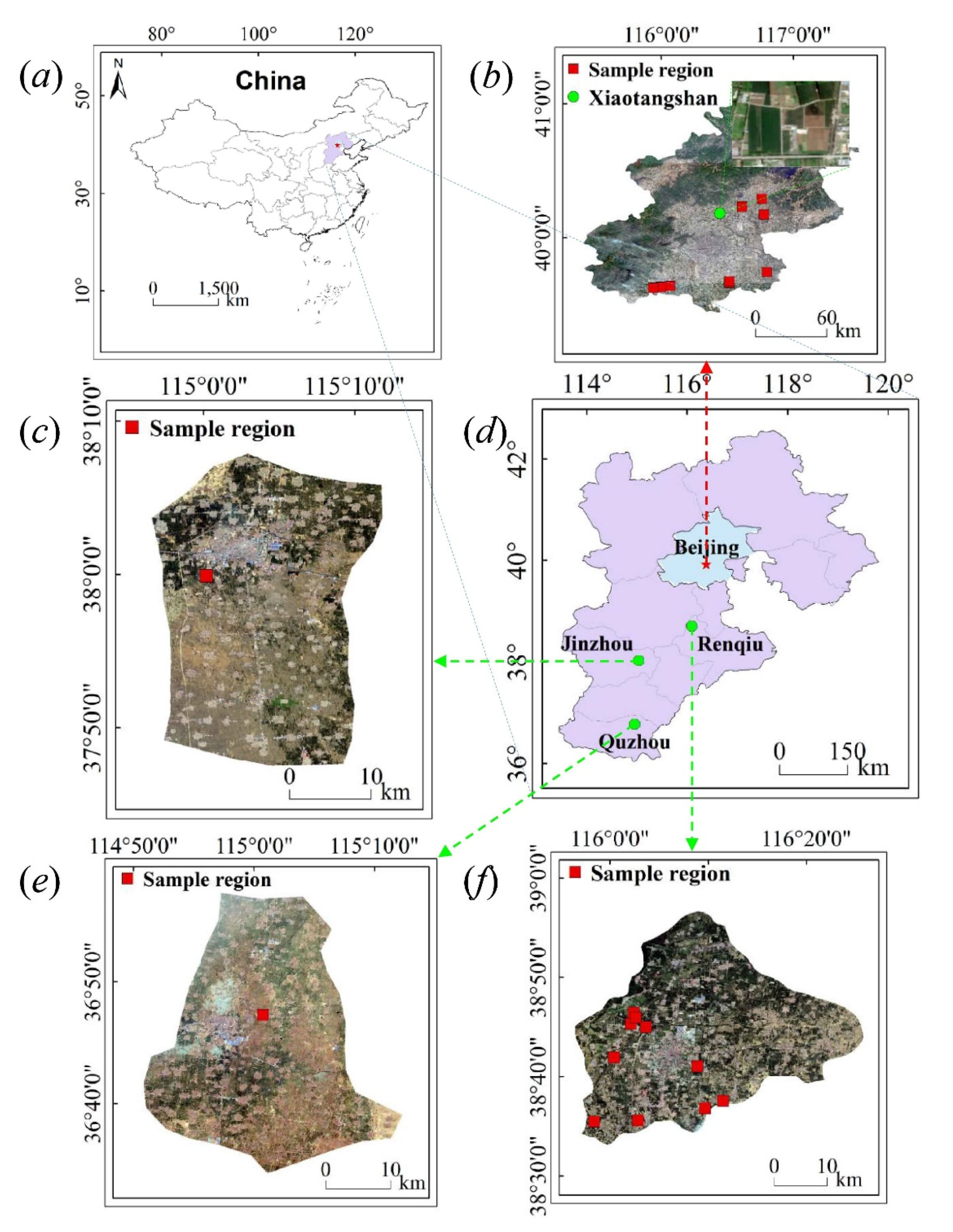
2.1. Research Area

The research areas are located in Xiaotangshan National Precision Agriculture Demonstration base in Changping District and suburbs of Beijing (BJ: 40°10′31″–40°11′18″N, 116°26′10″–116°27′05″E, altitude of 36 m), Renqiu (RQ: 38°33′–38°57′N, 115°56′–116°26′E, altitude of 4.5–11 m), Jinzhou (JZ: 37°47′30″–38°09′30″N, 114°58′20″–115°12′30″, altitude of 35–45 m), and Quzhou (QZ: 36°35′43″–36°57′N, 114°50′22.3″–115°13′27.4″E, altitude of 35–45 m) of Hebei Province (Figure 1). These areas are located in the north of the North China Plain, with a typical warm temperate monsoon climate, with obvious changes in the four seasons. There is strong evapotranspiration in spring, high temperature and frequent waterlogging in summer, and dry, windy, and cold winter. The annual average temperature and rainfall in BJ, RQ, JZ, and QZ are 11.8 °C and 550.3 mm, 12.1 °C and 557.4 mm, 12.5 °C and 554.6 mm, and 13.1 °C and 556.2 mm, respectively.

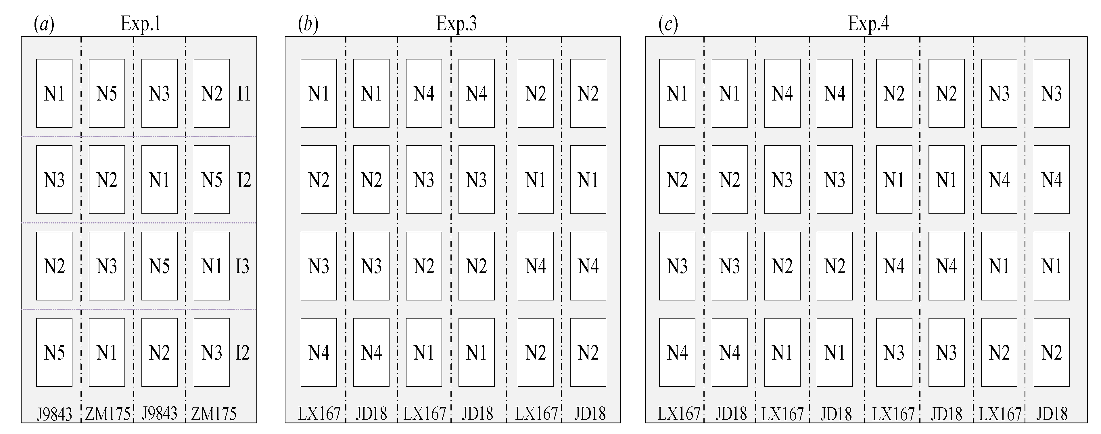
2.2. Experimental Design

A total of experiments was carried out at different regions and years. The experimental (Exp.) variables included different cultivars, irrigation rates, and application levels of nitrogen fertilizer (

Table 1. Summary of the experiment (Exp.) in this study.

Exp.	Antithesis	Site	Image	Cultivar	Application	Sample
Exp.1	2014.05.05	Xiaotangshan	RapidEye	J9843 1	Modeling	16
				ZM175 2
Exp.2	2015.05.18	Xiaotangshan	Landsat-8	— 1	Modeling	26
Exp.3	2017.05.16	Xiaotangshan	RapidEye	LX167 1	Modeling	24
				JD18 2
Exp.4	2018.05.08	Xiaotangshan	RapidEye	LX167 1	Modeling	31
				JD18 2
Exp.5	2018.05.08	Xiaotangshan	Sentinel-2	unknown 1	Validation	10
Exp.6	2019.05.13	Xiaotangshan	Sentinel-2	unknown 2	Validation	15
Exp.7	2018.05.08	Beijing	Sentinel-2	unknown 2	Validation	9
Exp.8	2018.05.08	Jinzhou	Sentinel-2	unknown 2	Modeling	6
Exp.9	2018.05.08	Quzhou	Sentinel-2	unknown 2	Modeling	6
Exp.10	2018.05.08	Renqiu	Sentinel-2	unknown 2	Validation	10

¹ and ² represent strong and medium gluten, respectively; the gluten information of unknown cultivar areas was provided by local seed departments and extension stations.

). Other field practices include weed and pest management, phosphate and potassium fertilizer, which were followed with local management procedures.

Exp. 1 was designed in Xiaotangshan (XTS) from 2013–2014 as an orthogonal design with two wheat cultivars (J9843 and ZM175), three irrigation rates (0, 146, and 292 mm), and four nitrogen fertilizer application rates (0, 90, 180, and 360 kg/hm²). A total of 16 plots were designed for modeling in this experiment (Figure 2a). The image data used in wheat flowering period were RapidEye (RE) satellite data.

Exp. 2 was designed with 26 samples for modeling in XTS during 2014–2015. The wheat variety was Jingdong22, and the amount of fertilizer applied was 90 kg/hm². The image data used in wheat flowering period were Landsat 8 Operational Land Imager (LS8) satellite data.

Exp. 3 was a completely randomized experiment designed in XTS during 2016–2017 for modeling with two wheat varieties (LX167 and JD18), four nitrogen fertilizer applications (0, 90, 180, and 270 kg/hm²), and three repetitions (Figure 2b). The image data used in wheat flowering period was RE satellite data.

Exp. 4 was a completely randomized experiment designed in XTS during 2017–2018 for modeling with two wheat varieties (LX167 and JD18), four nitrogen fertilizer applications (0, 90, 180, and 270 kg/hm²), and four repetitions (Figure 2c). The image data for the flowering period of wheat were the RE satellite data, which was used for consistency testing in addition to modeling.

Exp. 5 and 6 were designed in XTS during 2017–2018 and 2018–2019, respectively. The above-mentioned experiments were designed with 10 and 15 sample collection areas, and the image data were all Sentinel-2 (S2). S2 image data of both experiments were used for verification, and Exp. 5 was also used for consistency test with RE image data of Exp. 4.

Exp. 7–10 was designed during 2017–2018 in BJ, JZ, QZ, and RQ. The above-mentioned experiments were designed with 9, 6, 6, and 10 sample collection areas, and the image data were all S2. Exp. 8 and 9 were used for modeling, Exp. 7 and 10 were used for validation.

2.3. Data Acquisition

2.3.1. Satellite Image Preprocessing

Three RS satellite imageries, including S2, LS8, and RE, were used in this study (

Table 2. Overview of satellite information.

Name	Track Height (km)	Revisit Cycle (d)	Sensor	Band Number	Band Range (μm)	Spatial Resolution (m)
S2	786	5	Multispectral Imager (MSI)	13	0.4~2.4	10 (4 bands) 20 (6 bands) 60 (3 bands)
LS8	705	16	Operational Land Imager (OLI)	9	0.4~1.4	30 (Multispectral) 15 (Panchromatic)
			Thermal Infrared Sensor (TIRS)	2	10.6~12.5	100
RE	630	1	Push-broom Multispectral Imager	5	0.4~0.9	5

). A total of 12 images were collected, and a total of 10 images were used in Exp.1–10. The acquisition time was consistent with the antithesis in Table 1. Two more are S2 and LS8 on 28 April 2018 for conformance testing, and the spectral reflectance of the images for modeling and verification was extracted on the basis of the ground GPS coordinate information (Table 1). We collected the same day imaging data of different satellites in the same area, and extract the spectral reflectance of ground objects after geographical registration to test the spectral consistency of different satellites. In this study, S2 and LS8 images of XTS were acquired on 28 April 2018, and S2 and RE images of XTS were acquired on 8 May 2018. We obtained the wheat planting areas of BJ (11,270 ha) and RQ City (22,000 ha) from the National Bureau of Statistics to verify the accuracy of the wheat classification map.

S2 satellite is a multispectral RS imaging mission in the Global Environment and Safety Monitoring System (GMES) launched on 23 June 2015 and 7 March 2017, respectively. The single-star revisit period is 10 days, and the A/B double-star shortened the revisit period to 5 days. S2 images in this study were L1C level products downloaded from the ESA website (https://scihub.copernicus.eu/). Radiation calibration and atmospheric correction were performed using Sen2cor (http://link.zhihu.com/?target=http%3A//step.esa.int/main/third-party-plugins-2/sen2cor/), which is a L2A level data processing plug-in released by the ESA.

The LS8 satellite was successfully launched by NASA on 11 February 2013. LS8 data in this study were obtained from the USGS website (http://glovis.usgs.gov/). The imagery data were LIT products and geometrically corrected by terrain data. The image data were radiometrically calibrated and atmospherically corrected using ENVI 5.3 (Harris Geospatial, Broomfield, CO, USA) to use the spectral information.

The German RE satellite was launched on 29 August 2008 and consists of five Earth observation satellites. The five satellites are evenly distributed in a sun-synchronous orbit. RE 3A products were downloaded in this study. These products have been orthorectified, and the geographical accuracy of these products can reach 1–2 pixels. Image pre-processing was only atmospherically corrected in ENVI 5.3.

Supervised classification of winter wheat in BJ and RQ City was carried out using the 2017 Winter S2 image. The preprocessed images of the wheat flowering period in the two cities were masked with the classified images. Subsequently, the classified S2 and meteorological data for spatial verification were stacked. The above-mentioned operations were all implemented by ENVI 5.3.

2.3.2. Meteorological Data

The meteorological data of each experimental area were obtained from the ECMWF (http://www.ecmwf.int/). ECMWF provides global scale raster meteorological data with resolutions of 1°, 0.5°, 0.25°, and 0.125°. The ERA-Interim data at 0.125° resolution of the meteorological data was used in this work. Such data mainly included the daily rainfall, solar radiation, and minimum and maximum temperatures. The duration of the downloaded meteorological data is one month (30 days) before the imaging time of the image data selected for the flowering period of each growing season. For example, the imaging time of the S2 image used in the flowering period in 2018 is 8th May, and the time period of meteorological data is 8 April to 8 May 2018. The meteorological data were applied to the model in the form of total rainfall, total solar radiation, and accumulated temperature over this period. The main reason for choosing this period is that the time from stem growth to flowering of wheat in the study area is about one month (regardless of year), and the time of one month is practical in order to acquire meteorological data for regional applications. In this study, Python 3.7 (Python Software Foundation, Inc., Portland, USA) was used to download the meteorological data. MATLAB 2014 (MathWorks, Inc., Natick, USA) was used to read and standardized such data. ArcGIS 10.2 (Esri, Inc., Redlands, CA, USA) was used to add coordinate information and projections to raster meteorological data and for resampling.

2.3.3. Grain Protein Content (GPC)

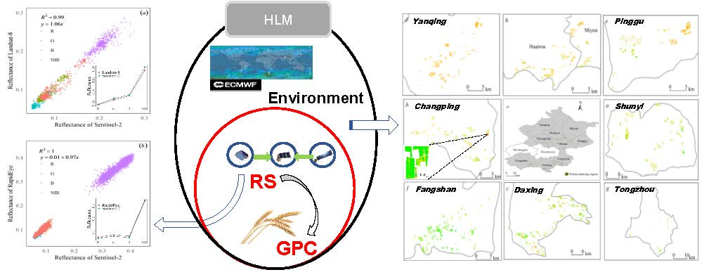
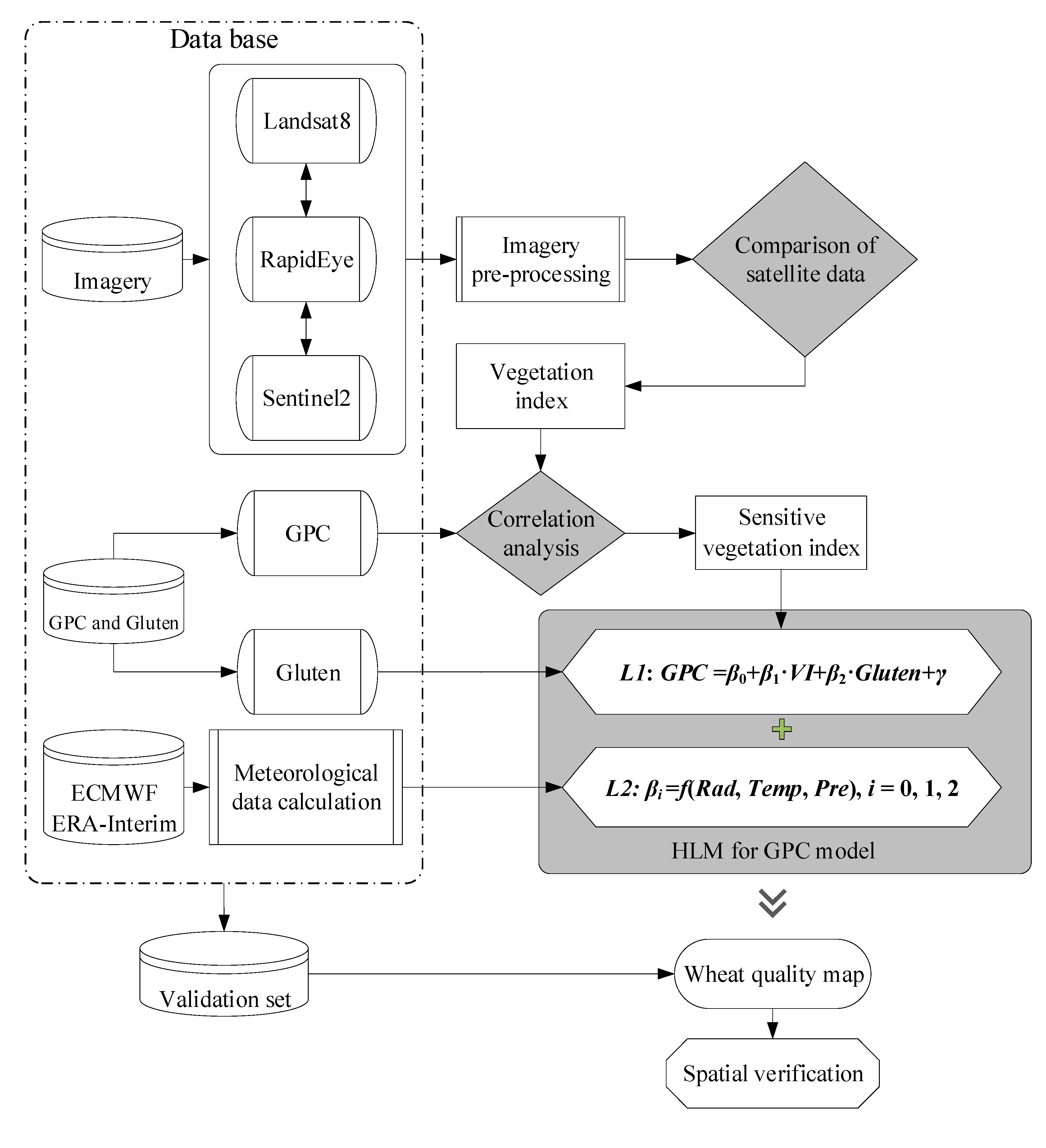
At harvest, 1 m² of the winter wheat was collected using the diagonal sampling method to measure the yield and grain quality. Each sample was at least 2 m away from the field edge to avoid the edge effect. After weighing by electronic, the GPC was measured with an Infratec TM 1241 near-infrared grain analyzer (FOSS A/S, Hillerød, Denmark).

2.4. Method

The illustrated methodology of the GPC prediction is general in Figure 3. The detailed steps are presented as follows:

(1)

Data pre-processing: The LS8, RE, and S2 RS image data were preprocessed (e.g., radiation calibration and atmospheric correction). The spectral information that corresponds to the ground point was extracted. Accumulated temperature, cumulative rainfall, and light intensity were calculated from the meteorological data.

(2)

Consistency analysis: The consistency of the spectral information of the preprocessed LS8 and RE with S2 was compared.

(3)

Vegetation index (VI) selection: The sensitive VI with GPC was calculated and screened from the RS images as the first input parameter of HLM.

(4)

GPC prediction by HLM method: The selected VI and gluten type were used as the first input parameters, and the meteorological data were used as the second input parameter to construct the HLM for predicting GPC;

(5)

GPC map and validation: The validation set was used to validate the HLM in space. The GPC in BJ, XTS, and RQ City in 2018 was predicted, and the thematic map of wheat quality prediction was created.

2.4.1. Vegetation index (VI)

Previous studies indicated that 10 vegetation indices with high correlation with protein were selected (

Table 3. Summary of vegetation index (VI) listed in this study. R, G, B, and NIR represent the reflectance of the satellite in the red, green, blue, and near infrared bands, respectively.

VI	Full Name	Formulation	Reference
DVI	Difference VI	$\mathrm{DVI}=\mathrm{NIR}-\mathrm{R}$	[39]
EVI	Enhanced VI	$\mathrm{EVI}=2.5\frac{\left(\mathrm{NIR}-\mathrm{R}\right)}{\left(\mathrm{NIR}+6\mathrm{R}-7.5\mathrm{B}+1\right)}$	[40]
GNDVI	Green normalized difference VI	$\mathrm{GNDVI}=\frac{\mathrm{NIR}-\mathrm{G}}{\mathrm{NIR}+\mathrm{G}}$	[41]
GRVI	Green ratio VI	$\mathrm{GRVI}=\frac{\mathrm{NIR}}{\mathrm{G}}$	[42]
IPVI	Infrared percentage VI	$\mathrm{IPVI}=\frac{\mathrm{NIR}}{\mathrm{NIR}+\mathrm{R}}$	[43]
MSR	Modified simple ratio	$\mathrm{MSR}=\frac{\left(\frac{\mathrm{NIR}}{\mathrm{R}}\right)-1}{\left(\sqrt{\frac{\mathrm{NIR}}{\mathrm{R}}}\right)+1}$	[44]
NDVI	Normalized difference VI	$\mathrm{NDVI}=\frac{\mathrm{NIR}-\mathrm{R}}{\mathrm{NIR}+\mathrm{R}}$	[45]
OSAVI	Optimized soil adjusted VI	$\mathrm{OSAVI}=\frac{\left(\mathrm{NIR}-\mathrm{R}\right)}{\left(\mathrm{NIR}+\mathrm{R}+0.16\right)}$	[46]
SAVI	Soil adjusted VI	$\mathrm{SAVI}=\frac{1.5\left(\mathrm{NIR}-\mathrm{R}\right)}{\left(\mathrm{NIR}+\mathrm{R}+0.5\right)}$	[47]
VARI	Visible atmospherically resistant index	$\mathrm{VARI}=\frac{\mathrm{G}-\mathrm{R}}{\mathrm{G}+\mathrm{R}-\mathrm{B}}$	[48]

). The correlation between each VI and GPC was analyzed. Subsequently, the optimal VI was selected to create the GPC model.

2.4.2. Hierarchical Linear Model (HLM)

The HLM is a least square regression analysis that considers data nested structures (e.g., the students are embedded in classes). However, the HLM can layer and comprehensively analyze the non-independent data, as well as the relationships between the data inside and outside the layer compared with the general least squares regression analysis, within a layer. At present, HLM has been extensive used in the field of education [49], economics [50], and agriculture [1].

The influence of environmental factors (layer 2 model) between regions and growth years on the grain quality will cause difference between RS information and grain quality model (layer 1 model, L1) considering the construction of regional and interannual GPC model. Therefore, HLM is feasible for the prediction and modeling of grain quality. In this study, the layer 1 model is constructed on the basis of the GPC, VI, and grain gluten type. The layer 2 model (L2) is constructed on the basis of the model coefficients in the L1 and the meteorological data, such as temperature (T), precipitation (Pre), radiation quantity (Rad) as follows:

$${L1:\mathrm{GPC}}_{\mathrm{ij}}{=\beta }_{0\mathrm{j}}{+\beta }_{1\mathrm{j}}\times \left({\mathrm{Glu}}_{\mathrm{ij}}\right){+\beta }_{2\mathrm{j}}\times \left({\mathrm{VI}}_{\mathrm{ij}}\right){+r}_{\mathrm{ij}}$$

(1)

where GPC_ij is the GPC; Glu and VI_ij represent the gluten type of winter wheat (the value of strong, medium strong, and weak gluten were 1, 2, and 3 in this study, respectively), and VI, respectively; β_0j, β_1j, and β_2j correspond to the intercept, the coefficients of gluten type, and VI, respectively; r_ij represents the random error; and i is the individual sample size.

$${L2:\beta }_{\mathrm{pj}}{=\gamma }_{\mathrm{p}0}{+\gamma }_{\mathrm{p}1}{\times Rad}_{\mathrm{j}}{+\gamma }_{\mathrm{p}2}{\times Pre}_{\mathrm{j}}{+\gamma }_{\mathrm{p}3}{\times T}_{\mathrm{j}}{+\mu }_{\mathrm{pj}}$$

(2)

where β_pj represents the intercept and the coefficients of gluten type and VI in the first layer; γ_p0 is the intercept of the second layer model; γ_p1, γ_p2, and γ_p3 are the model coefficients of total radiation, total precipitation, and accumulated temperature in this model, respectively; μ_pj represents the random error; p is the number of coefficient terms of L1, corresponding to 0, 1, and 2 in this study; and j is the individual sample size. The models of the winter wheat grain protein were developed by HLM 7.03 Student (www.ssicentral.com/hlm/student.html) software.

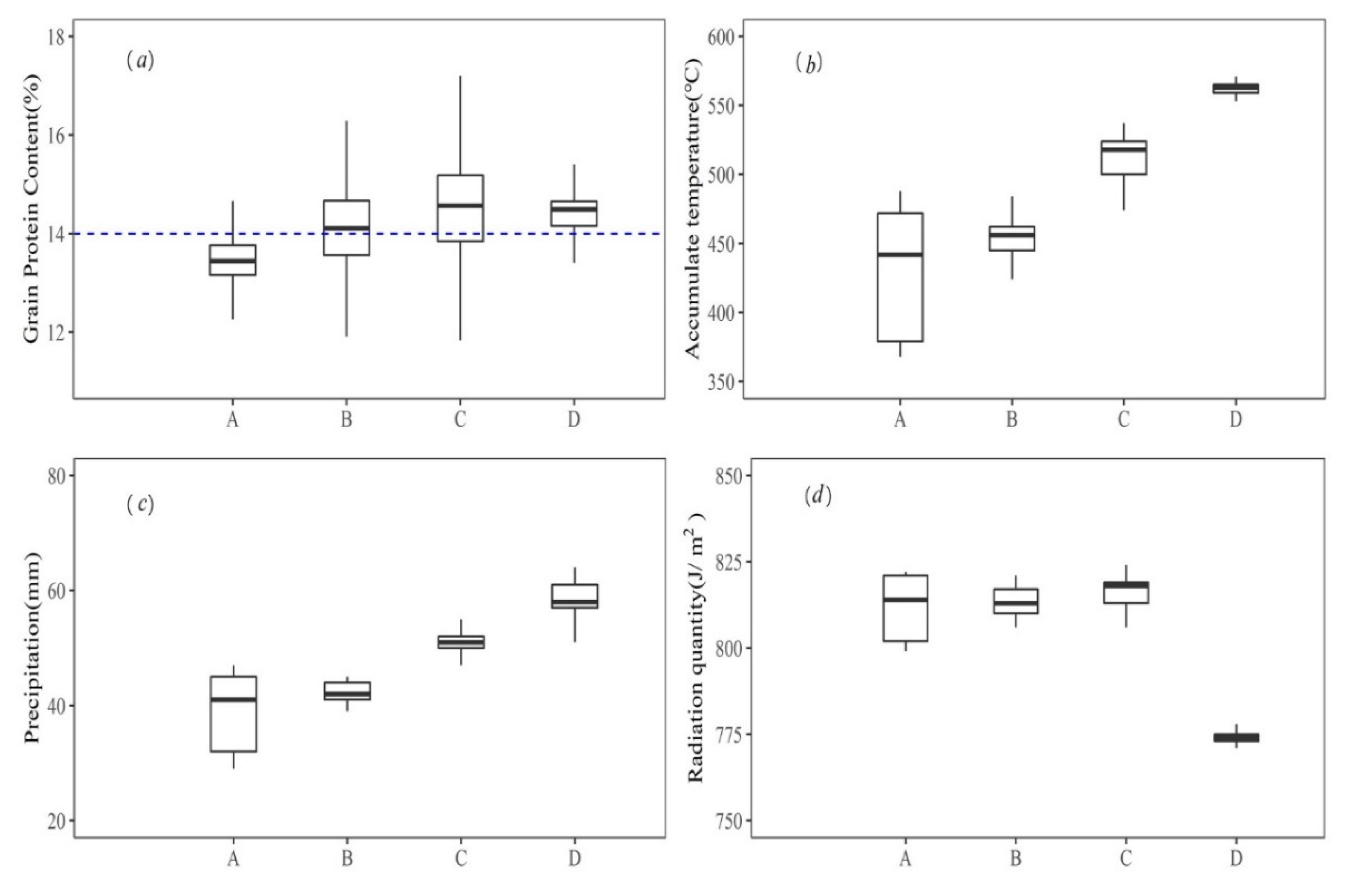
2.4.3. Classification Standard of Gluten

The national standard for high quality strong-gluten wheat (GB/T 17892-1999) (https://gb-standards.com/GB_standard/GB-T%2017892-1999.html) is adopted in this study. This standard specifies the definition, classification, quality index, inspection method, inspection rules, packaging, transportation, and storage requirements of wheat. The gluten types were classified as weak gluten (GPC ≤ 12%), medium gluten (12% < GPC ≤ 14%), strong gluten of the 2nd grade (14% < GPC ≤ 15%), and strong gluten of the 1st grade (15% < GPC) according to the standard of GPC in this study.

2.4.4. Statistical Analysis

In this study, the coefficient (R²), RMSE and relative root mean square error (rRMSE) were determined to verify the reliability and accuracy of the model [51]. The optimal VI based model is also established. Confusion matrix [52] and the accuracy indexes (ACC) are used to evaluate the effectiveness of GPC classification results.

$$\mathrm{RMSE}=\sqrt{\frac{1}{n}{\displaystyle \sum }_{i=1}^n{\left(Y_i{-Y}_i^{\text{’}}\right)}^2}$$

(3)

$$\mathrm{rRMSE}=\sqrt{\frac{1}{n}{\displaystyle \sum }_{i=1}^n{\left(\frac{Y_i{-Y}_i^{\text{’}}}{Y_i}\right)}^2}\times 100\%$$

(4)

$$\mathrm{ACC}=\frac{a_{ii}}{n}\ast 100\%$$

(5)

where n is the number of observations; Y_i and Y’_i are the ith measured and simulated data, respectively; ACC is the accuracy, it can directly reflect the correct proportion of classification, and the calculation is simple; $a_{ii}$ is the sum of correctly classified samples; n is the sample size; the degree of model fit is high when R² value is close to 1; the model prediction ability is strong, the stability is good, and the reliability is high when the RMSE and rRMSE value is small.

3. Results and Analysis

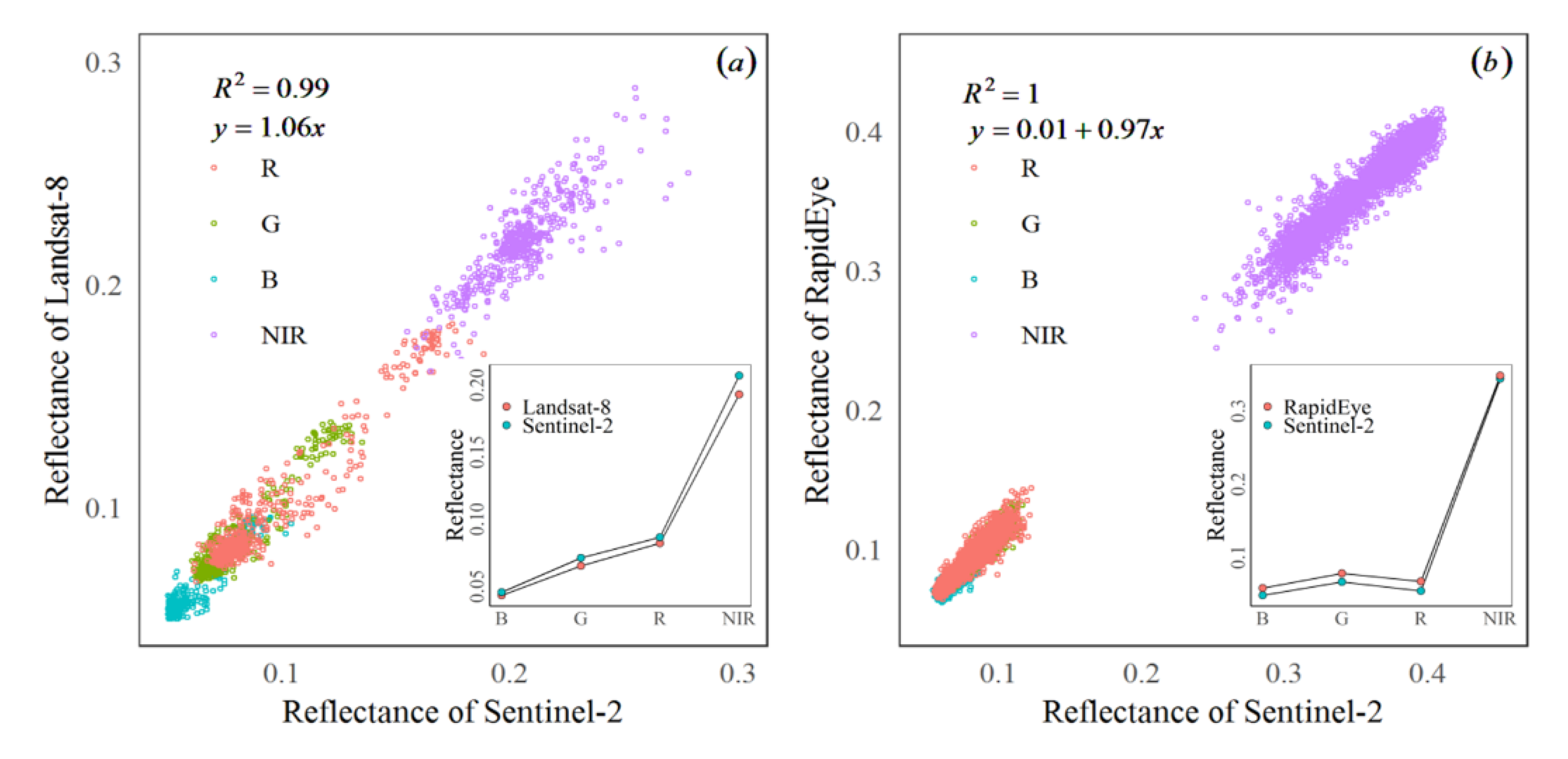
3.1. Spectral Consistency among Sentinel-2 (S2), Landsat 8 (LS8), and RapidEye (RE)

The spectral reflectance of different satellites in the same area and on the same day is extracted to verify the feasibility of multi-source remote sensing satellite complementation. The S2 and LS8 data, and the S2 and RE data were compared, respectively, to validate the data consistently among different sensors (Figure 4). Based on S2 imagery on 28 April 2018, LS8 imagery was georegistered. The S2 and LS8 imagery were resampled to 30 m resolution, the band reflectivity of 447 pixels was extracted for comparison, and the R² value was 0.99. Based on S2 imagery collected from 8 May 2018, RE imagery was georegistered. The S2 and RE imagery was resampled to 10 m resolution. The band reflectivity of 4165 pixels was extracted for comparison, and the R² value was 1.00. The average reflectivity of the four bands of the two groups of images was calculated and compared individually. The results show minimal difference between the two groups. The high consistency between S2 and LS8/RE demonstrated that these multisources could be used to construct a GPC model directly.

3.2. Screening of VI

The results showed that the selected VI and GPC were positively correlated (

Table 4. Correlation between VI and grain protein content (GPC) (n = 109).

VI	GPC	VI	GPC
DVI	0.46 **	MSR	0.42 **
EVI	0.48 **	NDVI	0.43 **
GNDVI	0.40 **	OSAVI	0.44 **
GRVI	0.40 **	SAVI	0.41 **
IPVI	0.43 **	VARI	0.39 **

** indicates extremely significant correlation (p < 0.01).

). The correlation reached a significant level (p < 0.01). EVI (r = 0.48) has the highest correlation, followed by DVI (r = 0.46), OSAVI (r = 0.44), VARI (r = 0.39). VARI (r = 0.39) has the worst correlation. Therefore, EVI was selected as an independent variable to participate in the construction of the winter wheat grain protein model.

3.3. GPC Predicting Model Based on HLM

The accuracy of the use of EVI to construct linear regression model (LR) for GPC was poor, with R² of 0.286, RMSE values of 1.11%, and rRMSE values of 8.63% (Figure 5b). Serious overestimates of the predicted GPC in winter wheat were shown during the 2014 and 2015 growing seasons. By contrast, the predicted GPC in the 2017 and 2018 growth seasons was underestimated. The model was insufficiently stable, and its performance greatly varied among different years and regions. The selected EVI and gluten data were considered the first layer information in HLM for GPC. Meteorological factors were considered the second layer information in HLM for GPC (

Table 5. Parameters of the hierarchical linear model for predicting GPC.

Fixed Effect	γp0	γp1	γp2	γp3
For intercept (β0j)	165.022	0.092	−0.223	−0.224
For Glu (β1j)	−45.730	−0.043	0.074	0.067
For VI (β2j)	−128.380	−0.007	0.157	0.220

). The parameters in Table 5 correspond to the parameters in Equations (1) and (2), and γ_p1, γ_p2, and γ_p3 explain the contribution of Rad, Pre, and T, respectively. β_0j, β_1j, and β_2j explain the influence of meteorological data on slope and intercept of gluten and VI. The GPC model based on the HLM method had better performance, with R² of 0.524, RMSE of 1.00%, and rRMSE of 8.12% (Figure 5a), than GPC model by LR method. Minimal difference was observed between the measured and the predicted values. The predicted results were reliable, especially the corrected accuracy interannual and regional scales.

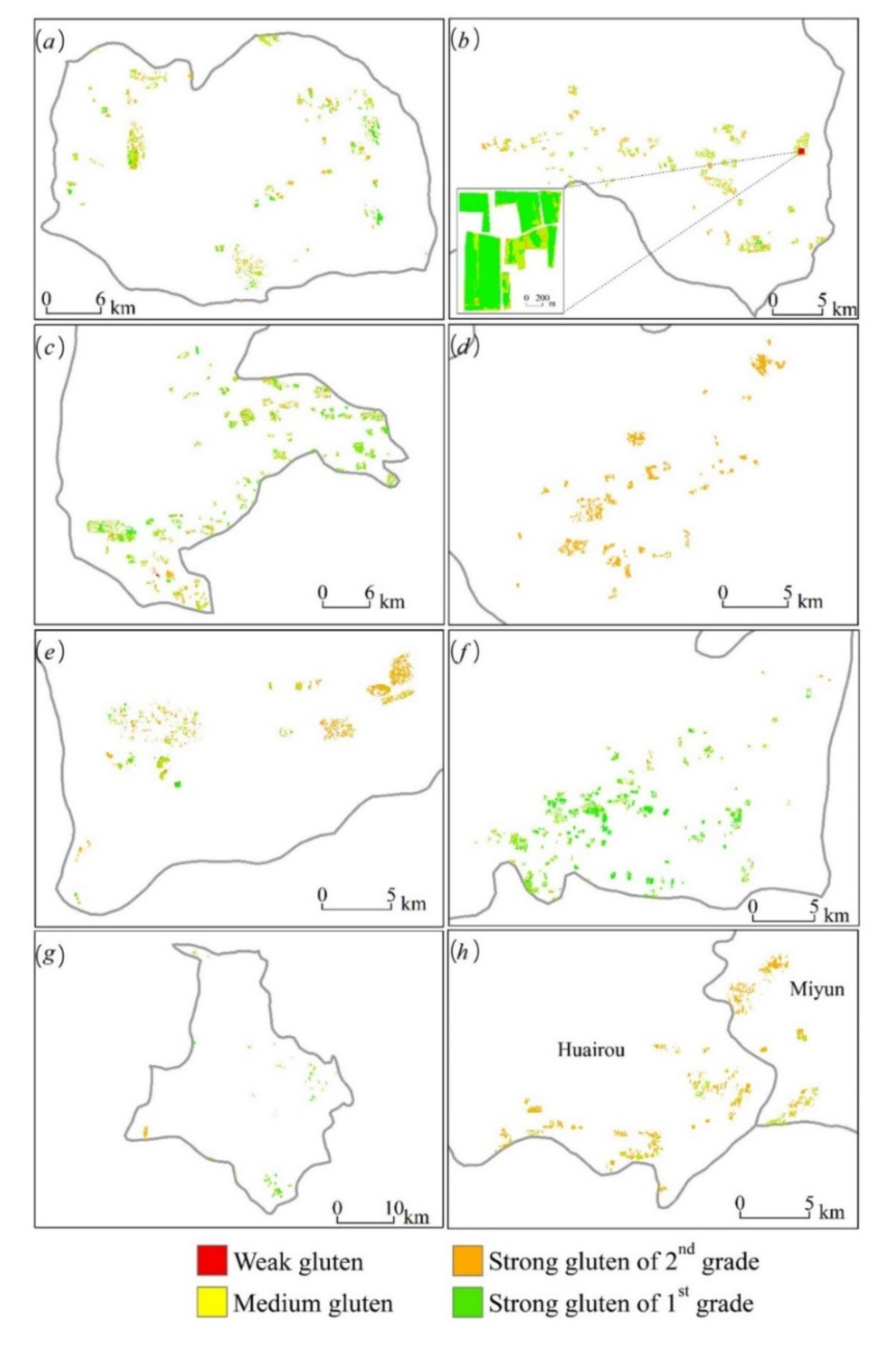
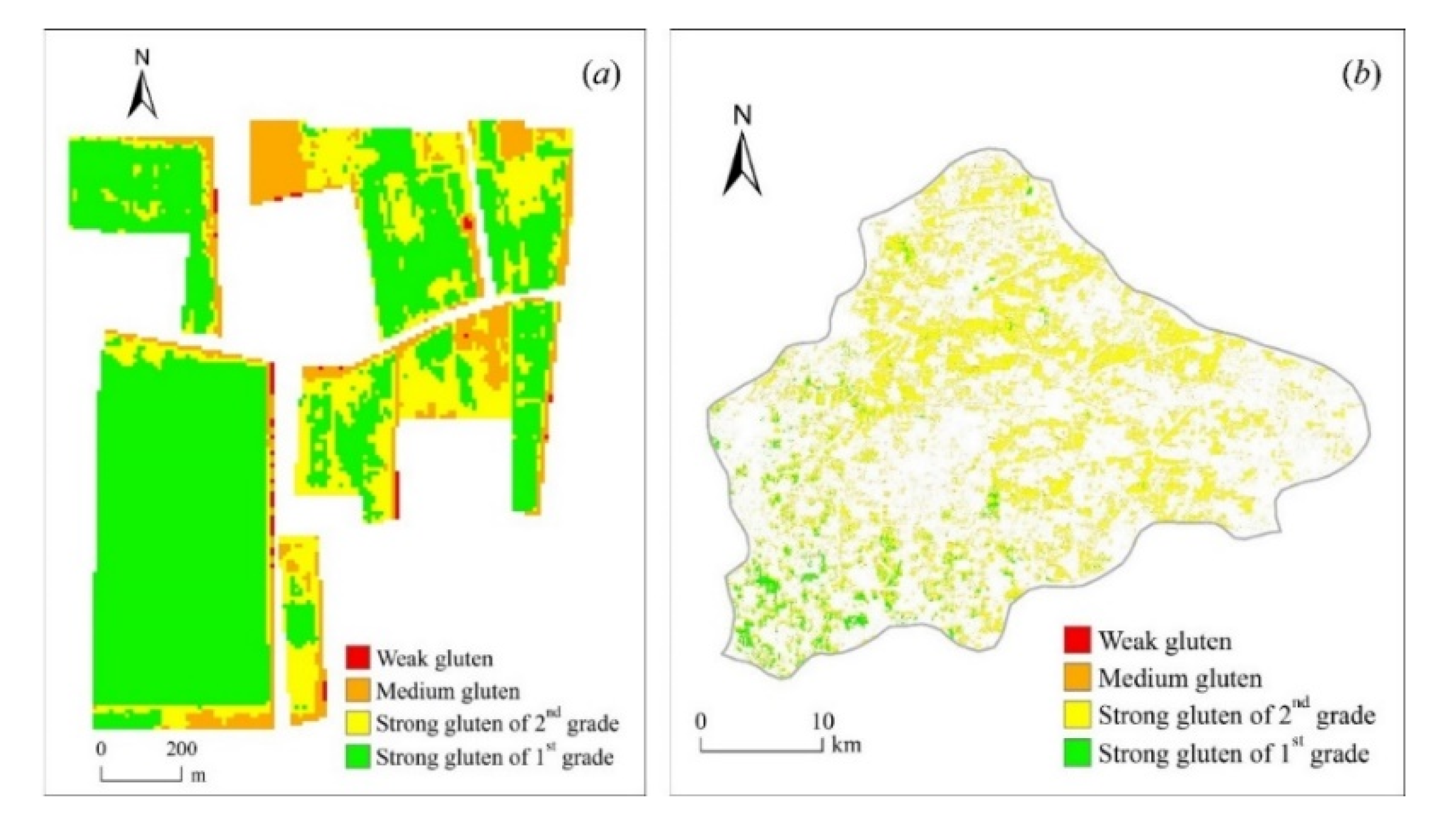
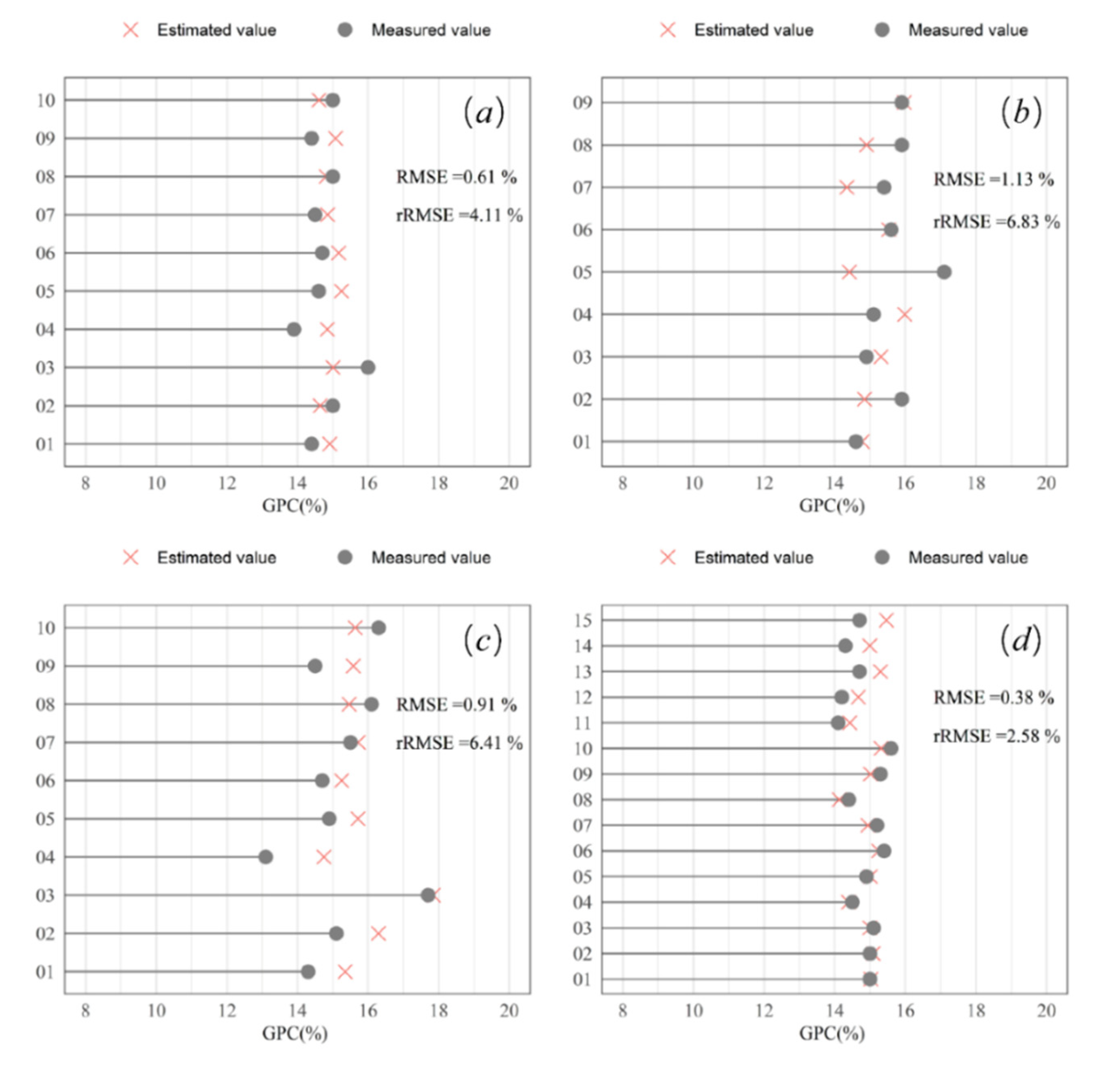
3.4. GPC Validation and Map

Figure 6 exhibits a wheat classification map based on winter S2 data. The planting areas of wheat in the statistical classification map were 12,448.44 ha in BJ City (Figure 6a) and 23,902.49 ha in RQ City (Figure 6b). These data were similar to those provided by the National Bureau of Statistics (11,270 and 22,000 ha). This finding showed that our classification was reliable. The figures and statistical data revealed that the wheat planting area in BJ was relatively small, mainly concentrated in Shunyi, Changping, Daxing, and Pinggu District, a small number of areas in Yanqing, Fangshan, and Tongzhou, and in the southern areas of Huairou and Miyun. The wheat planting in RQ City is relatively uniform. This work aims to integrate meteorological data for achieving regional GPC inversion.

The GPC at the flowering stage in 2018 and 2019 was predicted by using the constructed GPC monitoring model by HLM according to the fusion data of S2 satellite and raster meteorological data of winter wheat producing areas (Figure 7 and Figure 8). The gluten types were classified as weak gluten (GPC ≤ 12%), medium gluten (12% < GPC ≤ 14%), strong gluten of the 2nd grade (14% < GPC ≤ 15%), and strong gluten of the 1st grade (15% < GPC) according to the national standard for high quality strong-gluten wheat (GB/T 17892-1999). The image exhibits that the medium and strong gluten were dominant in both places. The area ratio of different gluten wheat in the image was counted (

Table 6. Statistics of wheat area with different gluten types.

Gluten	Weak Gluten	Medium Gluten	Strong Gluten of 2nd Grade	Strong Gluten of 1nd Grade
2018Beijing	0.71%	46.35%	34.47%	18.47%
2018Xiaotangshan	0%	3.40%	19.48%	77.12%
2019Xiaotangshan	0.72%	12.60%	25.20%	61.48%
2018Renqiu	0%	19.62%	72.56%	7.83%

Note: 2018Beijing indicates Beijing in 2018, other similar.

), and relatively small amount of weak gluten wheat was found in both places. The area ratio of medium gluten wheat in BJ was 46.35%, followed by strong gluten of the 2nd grade and 1st grade occupying an area of 34.47% and 18.47%, respectively. During 2017–2018, XTS, as the experimental base, was dominated by high quality strong gluten of the 1st grade wheat with an area ratio of 77.12%, followed by strong gluten of 2nd grade and medium gluten with an area of 19.48% and 3.40%, respectively. During 2018–2019, XTS was dominated by high quality strong gluten of the 1st grade wheat with an area ratio of 61.48%, followed by strong gluten of 2nd grade and medium gluten with an area of 25.20% and 12.60%, respectively. RQ City was dominated by strong gluten of 2nd grade wheat, occupying an area of 72.56%, followed by medium gluten occupying an area of 19.62%. The strong gluten level-1 was less, with an area of 7.83%.

The S2 data of 44 points in RQ (10 points), BJ (9 points), XTS (10 points) in 2018, and XTS (15 points) in 2019 were used as verification sets. The predicted result was slightly different from the measured result, with RMSE values for RQ, BJ, XTS in 2018, and XTS in 2019 of 0.61%, 1.13%, 0.91%, and 0.38% and rRMSE values of 4.11%, 6.83%, 6.41%, and 2.58%, respectively (Figure 9). The results show that the HLM coupling environmental factors and gluten was reliable, based on the S2 image data. Large-scale wheat quality prediction could be carried out in the BJ–Tianjin–Hebei region. A technical basis for the wide range application of RS technology in predicting GPC on a spatial scale could be provided.

4. Discussion

Due to the first launch of S2 satellite in June 2015, the data of this study in 2015 cannot be used. Even after 2016, there would be insufficient data sources due to the long revisit cycle of a single satellite. For example, in a certain year, the flowering period in the suburb of Beijing is in the early May, and the S2 satellite in this area has no image in this period. Therefore, we tried to make up for this problem by complementing multiple satellites. Another advantage of introducing multi-source satellites was the ability to verify that our model can be unified for different sensors. If different satellite spectra were consistent, it was proved that our models can be used universally among different satellites. If the spectra were not consistent, new models needed to be established according to applied satellites. Due to different satellite sensors and different space scales, we must consider the problem of spectral consistency. We had explored the consistency test of multi-source satellite imageries, S2, LS8, and RE to enrich the RS data sources. Li et al. [53] attempted to study the potential of multispectral data for estimating biomass of non-photosynthetic vegetation. LS8 and S2 images were simultaneously used, but they were not tested for consistency. The study results showed that the differences between the aforementioned were small, and their spectral reflectance was highly consistent. This finding proved that the image data of the three imageries could participate in the model construction without correction processing. However, due to the cost, we did not analyze whether the band information between other satellites or sensors (e.g., high score satellite series and resource satellite series) was consistent. Further research will consider the consistency among other satellites, aviation platforms, and terrestrial platforms. By doing so, the RS image data will be further enriched, and a sufficient range of data sources in the application of regional GPC prediction will be ensured.

Researchers have carried out countless research in the field scale on GPC monitoring and proposed a series of methods and models. Hansen et al. [6] and Wang et al. [54] selected sensitive bands with high correlation with GPC to construct the model in the early stage. The model performance was poor because of the uncertainty of single band reflectance. Song et al. [55] showed that the best model for GPC prediction was index model, but R² was only 0.426 and 0.494. The follow-up researchers mostly used the VI to create models for effectively avoiding this uncertainty and predict GPC [9,56]. Feng et al. used multiple vegetation index to build GPC prediction model, in which the linear model constructed by modified normalized difference705 (mND705) has the highest precision with R² and RMSE values of 0.616 and 1.019%. However, this was based on the high-resolution ground hyperspectral data in precision agriculture. Similar accuracy based on satellite and field data was achieved in this study. The use of RS data only was insufficient for GPC prediction and would lead to the above-mentioned problem. This phenomenon was because of genotypes accounting for 95% and environmental factors accounting for 5% of the grain protein contribution [19]. The inherent basis of wheat quality characteristics depended on genotypes, which had different connotations, evaluation indicators, and suitable ecological regions with various product uses [57]. The genotype and environmental factors, namely variety information and meteorological data, were fully considered in this study. The GPC monitoring model was constructed by correlating RS data, species, and meteorological data with HLM. The HLM can effectively improve the GPC prediction accuracy by comparing the HLM and LR model constructed from RS data only. This conclusion was consistent with that of Wang et al. [2]. The GPC empirical model using RS data and environmental factors was more precise than the use of RS data or environmental factors alone. The HLM also effectively corrected inter-annual and inter-regional deviations. This outcome is attributed to this study regarding RS data, species, and meteorological data as two-layer nested structure data and decomposition of the total variance of GPC data by using the HLM. In this way, the interaction of different varieties and environments on GPC was considered, which played a key role in inter-annual and inter-regional deviation correction. Li et al. [28] also considered the influence of environment and gluten on GPC prediction, but mainly focused on the field scale and confirmed the HLM method for quality prediction interannual scales. This study was demonstrated at regional scales with some different results in the following aspects: (i) remote sensing data sources are different. We used the multi-source remote sensing satellite data (not the ground hyperspectral data), and analyzed the consistency of different remote sensing satellites to achieve the regional prediction of GPC; (ii) meteorological data are different. We used the grid meteorological data (not the data of a point), which provided the basis for large-scale GPC prediction; (iii) different experiments. We not only designed the plot experiment, but also conducted the random sampling experiment in the field, so it is more popularized. (iv) quality map is more useful to joint practical production.

However, there were still cases of gluten misclassification, e.g., weak gluten grains with high GPC value may be predicted as strong gluten of 2nd grade, and vice versa. We must point that GPC prediction during growing period is a rough classification to guide harvest. According to the standard of rough classification, we combined the strong gluten of 2nd grade and strong gluten of 1st grade into the strong gluten, and used the confusion matrix (

Table 7. Rough classification monitoring results (n = 153).

	Weak Gluten M	Medium Gluten M	Strong Gluten M
Weak Gluten E	2	1	0
Medium Gluten E	11	24	8
Strong Gluten E	2	16	89

^M,^E indicates measurement and estimation respectively.

) to evaluate the accuracy. The overall classification accuracy (ACC = 0.75) shows that the model can achieve positive classification results. However, due to the imbalance of the data set, there were limited samples of weak gluten in the modeling set, resulting in a large number of samples of weak gluten that were misclassified. A further study to balance the data set will improve this situation. Compared to the traditional non-classified harvest, GPC prediction and classification could improve the harvest grain quality, and even the misclassification has little percentage on the large proportion in one gluten type. Due to the sample size and GPC classification threshold (only 1% of the strong gluten of 2nd grade and strong gluten of 1st grade), a small number of misclassifications in the classification process caused a large deviation, which made it difficult to classify the strong gluten of 2nd grade and strong gluten of 1st grade. In addition, this study was based on the prediction of flowering stage, and the influence of other factors in the filling stage will also cause classification deviation. In spite of this, it can still have an important guiding significance for harvest classification. Sampling inspection during storage was necessary. Only the type of gluten needed to be determined at the fuzzy boundary of strong gluten wheat, which greatly reduced the workload of random inspection.

Feng et al. [58] indicated that the optimal prediction period was the flowering stage. The meteorological data only used the empirically selected accumulated temperature, solar radiation, and rainfall one month before the flowering period. Although the data achieved good results, it may be insufficient. This issue is attributed to the impact of HLM supported by various information and meteorological data on the prediction of the optimal growth stage and the VI in different GPC growth stages. The meteorological data not only included temperature, solar radiation, and rainfall. The following work will also consider other growth periods as the origin and analyze the types and time bucket sensitivity of the accumulated meteorological data before and after the origin. Such work will consider the phenological factors to establish a full-time GPC monitoring model. In addition, latitude, topography, and soil information need to be considered.

In terms of variety information, RQ and BJ, which were commonly planted medium-gluten varieties, were compared. The monitoring results in RQ City were mainly strong-gluten wheat (Figure 10a). The monitoring results in BJ show that medium and strong gluten were distributed. The northern mountain area of BJ was dominated by medium gluten (Figure 10a). The middle and strong gluten evenly distributed in the gentle zone in the middle (Figure 10a), and the strong gluten was mainly distributed in the south (Figure 10a). This difference was due to the varying meteorological factors in the four regions. This conclusion once again verified the accuracy of the starting point of our study. Such notion indicated that the response of varieties to diverse environments was vary. We calculated the meteorological data for the four regions (Figure 10b–d). The difference of accumulated temperature was the greatest in the four regions, and those of precipitation and radiation quantity were relatively stable. Figure 10a shows that the wheat GPC was high when the temperature was also high. This finding was consistent with the agronomic conclusions of Guasconi et al. [19]. Figure 10c shows that the precipitation and GPC were high when the latitude was also high. However, previous studies [20] showed that GPC was inversely proportional to precipitation, which was inconsistent with our statistics. This similarity may be due to the small precipitation gradient difference in each region. Moreover, the interaction between temperature and precipitation affects the results. Therefore, the relationship between single climatic factors and GPC should be investigated, and the adverse effects between various factors cannot be ignored. Figure 10d shows that the radiation quantity of the three areas in BJ is the same, while that of RQ is low. The effect of radiation quantity on the difference of GPC cannot be verified.

The genotype and environmental interaction should be fully considered in various selection and field management. Various promoters should extend the different genotypes to their suitable ecological areas in the future. The varieties used in this study were mainly strong gluten and medium-strong gluten, and the weak gluten was seldom used. The modeling set was insufficiently diversified in the gluten. Additional weak gluten wheat varieties will be considered to participate in the modeling in the future. The wheat gluten in our model was derived from the known variety information. However, the variety information was difficult to obtain in the actual regional prediction. Therefore, the variety information from the seed departments and their extension stations should be obtained to create the wheat variety flow direction and distribution map in the regional application.

5. Conclusions

In this study, a GPC monitoring model based on HLM was established by combining gluten, meteorological data, and multisource RS images. The poor interannual expansion and regional transfer of the traditional models were corrected effectively. The major study conclusions are presented as follows: (1) LS8, RE, and S2 had high consistency in spectral information and could be combined for RS modeling; (2) The GPC prediction model based on HLM (R² = 0.524, RMSE = 1.00% and rRMSE = 8.12%) was better than the traditional linear model (R² = 0.286, RMSE = 1.11% and rRMSE = 8.63%). In combination with the meteorological data and gluten, the problem of spatiotemporal deviation was effectively corrected. (3) The GPC regional prediction of wheat in BJ and RQ was realized by using the model and S2 data. These results show that the potential of HLM in predicting GPC of winter wheat on the interannual and regional scales can provide technical reference for GPC prediction in global or regional scale.

References

1. Li, Z.; Wang, J.; Liu, C.; Song, X.; Xu, X.; Li, Z. Predicting Grain Protein Content in Winter Wheat Using Hyperspectral and Meteorological Factor. In Proceedings of the 2018 7th International Conference on Agro-geoinformatics (Agro-geoinformatics), Hangzhou, China, 6 August 2018; pp. 1–4. [Google Scholar]
2. Wang, D.; Zhang, D.; Li, Y.; Qin, Q.; Wang, J.; Fan, W.; Chen, S. Monitoring wheat quality based on HJ1A/B remote sensing data and ecological factors. Infrared Laser Eng. 2013, 42, 780–786. [Google Scholar]
3. Xue, L.-H.; Zhu, Y.; Zhang, X.; Cao, W. Predicting Wheat Grain Quality with Canopy Reflectance Spectra. Acta Agron. Sin. 2004, 30, 1036–1041. [Google Scholar]
4. Jin, X.; Xu, X.; Feng, H.; Song, X.; Wang, Q.; Wang, J.; Guo, W. Estimation of grain protein content in winter wheat by using three methods with hyperspectral data. Int. J. Agric. Biol. 2014, 16. [Google Scholar]
5. Liu, L.; Wang, J.; Bao, Y.; Huang, W.; Ma, Z.; Zhao, C. Predicting winter wheat condition, grain yield and protein content using multi-temporal EnviSat-ASAR and Landsat TM satellite images. Int. J. Remote Sens. 2006, 27, 737–753. [Google Scholar] [CrossRef]
6. Hansen, P.M.; Jorgensen, J.R.; Thomsen, A. Predicting grain yield and protein content in winter wheat and spring barley using repeated canopy reflectance measurements and partial least squares regression. J. Agric. Sci. -Camb. 2003, 139, 61–66. [Google Scholar] [CrossRef]
7. Li, Y.; Zhu, Y.; Tian, Y.; You, X.; Zhou, D.; Cao, W. Relationship of grain protein content and relevant quality traits to canopy reflectance spectra in wheat. Sci. Agric. Sin. 2005, 38, 1332–1338. [Google Scholar]
8. Rodrigues, F.A.; Gerald, B.; Pierre, B.D.; Ortiz-Monasterio, J.I.; Schulthess, U.; Zarco-Tejada, P.J.; Taylor, J.A.; Gérard, B. Multi-Temporal and Spectral Analysis of High-Resolution Hyperspectral Airborne Imagery for Precision Agriculture: Assessment of Wheat Grain Yield and Grain Protein Content. Remote Sens. 2018, 10, 930. [Google Scholar] [CrossRef] [Green Version]
9. Zhou, D.; Zhu, Y.; Yao, X.; Tian, Y.; Cao, W. Estimating Grain Protein Content with Canopy Spectral Reflectance in Rice. Acta Agron. Sin. 2007, 33, 1219–1225. [Google Scholar]
10. Pettersson, C.G.; Söderström, M.; Eckersten, H. Canopy reflectance, thermal stress, and apparent soil electrical conductivity as predictors of within-field variability in grain yield and grain protein of malting barley. Precis. Agric. 2006, 7, 343–359. [Google Scholar] [CrossRef]
11. Zhang, S.; Feng, M.; Yang, W.; Wang, C.; Sun, H.; Jia, X.; Wu, G. Detection of grain content in winter wheat based on near infrared spectroscopy. Chin. J. Ecol. 2018, 37, 1276–1281. [Google Scholar]
12. Zhao, C.; Li, Z.; Yang, G.; Duan, D.; Zhao, Y.; Yang, W. Remote Sensing Prediction of Grain Protein Content in Winter Wheat Based on Gluten Type Correction Coefficient. J. Triticeae Crop. 2020, 1–8. [Google Scholar]
13. Cox, M.C.; Qualset, C.O.; Rains, D.W. Genetic Variation for Nitrogen Assimilation and Translocation in Wheat. II. Nitrogen Assimilation in Relation to Grain Yield and Protein. Crop. Sci. 1985, 25, 737–740. [Google Scholar] [CrossRef]
14. Liu, D.Y.; Wu, J.X.; Ren, W.J.; Wu, J.X.; Yang, W.Y. Effects of nitrogen strategies on nitrogen uptake, utilization and grain quality of broadcasted rice under no-tillage with high standing-stubbles. Plant. Nutr. Fertil. Sci. 2009, 15, 514–521. [Google Scholar]
15. Huang, W.; Wang, J.; Liu, L.; Wang, Z.; Tan, C.; Song, X.; Wang, J. Study on grain quality forecasting method and indicators by using hyperspectral data in wheat. Proc. Spie Int. Soc. Opt. Eng. 2005, 5655, 291–300. [Google Scholar]
16. Chen, P.F.; Wang, J.S.; Pan, P.; Xu, Y.Y.; Yao, L. Remote detection of wheat grain protein content using nitrogen nutrition index. Trans. Chin. Soc. Agric. Eng. 2011, 9, 261–265. [Google Scholar]
17. Orlando, F.; Marta, A.D.; Mancini, M.; Motha, R.; Qu, J.J.; Orlandini, S. Integration of Remote Sensing and Crop Modeling for the Early Assessment of Durum Wheat Harvest at the Field Scale. Crop. Sci. 2015, 55, 1280. [Google Scholar] [CrossRef]
18. Cao, W.; Guo, W.; Wang, L. Physiological Ecology and Optimizing Technology of Wheat Quality; China Agriculture Press: Beijing, China, 2005. [Google Scholar]
19. Guasconi, F.; Dalla, M.A.; Grifoni, D.; Mancini, M.; Orlando, F.; Orlandini, S. Influence of climate on durum wheat production and use of remote sensing and weather data to predict quality and quantity of harvests. Ital. J. Agrometeorol. 2011, 16, 21–28. [Google Scholar]
20. Orlandini, S.; Mancini, M.; Grifoni, D.; Orlando, F.; Marta, A.D.; Capecchi, V. Integration of meteo-climatic and remote sensing information for the analysis of durum wheat quality in Val d’Orcia (Tuscany, Italy). Q. J. Hung. Meteorol. Serv. 2011, 115, 233–245. [Google Scholar]
21. Li, W.G.; Wang, J.H.; Zhao, C.J.; Liu, L.Y.; Song, X.Y.; Tong, Q.X. A model for predicting protein content in winter wheat grain based on Land-Sat TM image and nitrogen accumulation. J. Remote Sens. 2008, 12, 506–514. [Google Scholar]
22. Li, Z.; Xu, X.; Jing, X.; Zhang, J.; Song, X.; Song, S.; Yang, G.; Wang, J. Remote sensing prediction of winter wheat protein content based on nitrogen translocation and GRA-PLS method. Sci. Agric. Sin. 2014, 47, 3780–3790. [Google Scholar]
23. Li, M.; Observatory, S.M. Study of the Objective Probability Forecast Method for Short-Term Heavy Rain Based on ECMWF Fine-Mesh Model. J. Trop. Meteorol. 2017, 33. [Google Scholar]
24. Zhang, H.-L.; Wu, N.-G.; Tian, S.-Y.; Lin, F.-N. Verification and Analysis of Statistics of Rainfall Ensemble Forecast by ECMWF in Guangdong Province. Guangdong Meteorol. 2017, 3–8. [Google Scholar]
25. Alpert, P.; Neeman, B.U.; Shay-El, Y. Climatological analysis of Mediterranean cyclones using ECMWF data. Tellus A Dyn. Meteorol. Oceanogr. 1990, 42, 65–77. [Google Scholar] [CrossRef] [Green Version]
26. Wang, P. Verification and analysis on the rainstorm forecast performance of ECMWF high resolution numerical model in Guang’ an. Mid-Low Latit. Mt. Meteorol. 2018. [Google Scholar]
27. Huang, W.; Song, X.; Lamb, D.W.; Wang, Z.; Niu, Z.; Liu, L.; Wang, J. Estimation of winter wheat grain crude protein content from in situ reflectance and advanced spaceborne thermal emission and reflection radiometer image. J. Appl. Remote Sens. 2008, 2, 1220–1230. [Google Scholar] [CrossRef]
28. Li, Z.; James, T.; Hao, Y.; Raffaele, C.; Xiuliang, J.; Zhenhong, L.; Xiaoyu, S.; Guijun, Y. A hierarchical interannual wheat yield and grain protein prediction model using spectral vegetative indices and meteorological data. Field Crop. Res. 2020, 248. [Google Scholar] [CrossRef]
29. Pettersson, C.G.; Eckersten, H. Prediction of grain protein in spring malting barley grown in northern Europe. Eur. J. Agron. 2007, 27, 205–214. [Google Scholar] [CrossRef]
30. Song, X.; Wang, J.; Huang, W. Winter wheat growth and grain protein uniformity monitoring through remotely sensed data. Proc. Spie Int. Soc. Opt. Eng. 2010, 7824. [Google Scholar]
31. Li, C.; Zhang, R.; Guo, W.; Zhu, X.; Peng, Y. Relationship between HMW-GS and GMP Contents with Gluten Content in Wheat for Different End Use. J. Chin. Cereals Oils Assoc. 2009. [Google Scholar]
32. Guo, T.; Zhang, X.; Fan, S.; Zhu, Y.; Wang, C.; Ma, D. Effects of different environments on qualitative characters of three gluten wheat cultivars. Chin. J. Appl. Ecol. 2003, 14, 917. [Google Scholar]
33. Wilson, A.M.; Silander, J.A.; Gelfand, A.; Glenn, J.H. Scaling up: Linking field data and remote sensing with a hierarchical model. Int. J. Geogr. Inf. Sci. 2011, 25, 509–521. [Google Scholar] [CrossRef]
34. Wallach, D. Regional Optimization of Fertilization Using a Hierarchical Linear Model. Biometrics 1995, 51, 338–346. [Google Scholar] [CrossRef]
35. Shan, W.; Jin, X.; Meng, X.; Yang, X.; Xu, Z.; Gu, Z.; Zhou, Y. Dynamical monitoring of ecological environment quality of land consolidation based on multi-source remote sensing data. Trans. Chin. Soc. Agric. Eng. 2019, 35, 234–242. [Google Scholar]
36. Ma, J.; Zhang, C.; Lu, Y.; Gao, L.; Yun, W.; Zhu, D.; Chen, W.; Wang, H. Monitoring and evaluation of cultivated land quality supported by multi-source remote sensing. China Agric. Inform. 2018, 30, 18–26. [Google Scholar]
37. Zhao, J.; Li, J.; Liu, Q.; Fan, W.; Zeng, Y.; Xu, B.; Yin, G. Leaf area index inversion combining with HJ-1/CCD and Landsat 8/OLI data in the middle reach of the Heihe River basin. J. Remote Sens. 2015, 19, 733–749. [Google Scholar]
38. Ouyang, L.; Mao, D.; Wang, Z.; Li, H.; Man, W.; Jia, M.; Liu, M.; Zhang, N.; Liu, H. Analysis crops planting structure and yield based on GF-1 and Landsat8 OLI images. Trans. Chin. Soc. Agric. Eng. 2017, 33, 147–156. [Google Scholar]
39. Tucker, C.J. Red and photographic infrared linear combinations for monitoring vegetation. Remote Sens. Environ. 1979, 8, 127–150. [Google Scholar] [CrossRef] [Green Version]
40. Huete, A.; Didan, K.; Miura, T.; Rodriguez, E.P.; Gao, X.; Ferreira, L.G. Overview of the radiometric and biophysical performance of the MODIS vegetation indices. Remote Sens. Environ. 2002, 83, 195–213. [Google Scholar] [CrossRef]
41. Gitelson, A.A.; Merzlyak, M.N. Remote sensing of chlorophyll concentration in higher plant leaves. Adv. Space Res. 1998, 22, 689–692. [Google Scholar] [CrossRef]
42. Sripada, R.P.; Heiniger, R.W.; White, J.G.; Meijer, A.D. Aerial color infrared photography for determining early in-season nitrogen requirements in corn. Agron. J. 2006, 98, 968–977. [Google Scholar] [CrossRef]
43. Crippen, R.E. Calculating the vegetation index faster. Remote Sens. Environ. 1990, 34, 71–73. [Google Scholar] [CrossRef]
44. Chen, J.M. Evaluation of vegetation indices and a modified simple ratio for boreal applications. Can. J. Remote Sens. 1996, 22, 229–242. [Google Scholar] [CrossRef]
45. Rouse, J.W.; Haas, R.H.; Schell, J.A.; Deering, D.W. Monitoring vegetation systems in the Great Plains with ERTS. NASA Spec. Publ. 1974, 351, 309. [Google Scholar]
46. Rondeaux, G.; Steven, M.; Baret, F. Optimization of soil-adjusted vegetation indices. Remote Sens. Environ. 1996, 55, 95–107. [Google Scholar] [CrossRef]
47. Huete, A.R. A soil-adjusted vegetation index (SAVI). Remote Sens. Environ. 1988, 25, 295–309. [Google Scholar] [CrossRef]
48. Gitelson, A.A.; Stark, R.; Grits, U.; Rundquist, D.; Kaufman, Y.; Derry, D. Vegetation and soil lines in visible spectral space: A concept and technique for remote estimation of vegetation fraction. Int. J. Remote Sens. 2002, 23, 2537–2562. [Google Scholar] [CrossRef]
49. Lin, T.J.; Wu, W.; Yu, W.X.; Wang, J. Citizen’s Satisfaction with Public Education Service in China: A Quantitative Analysis via Hierarchical Linear Model. Fudan Educ. Forum 2011, 9, 54–58. [Google Scholar]
50. Qiao, R.-L.; Chen, L.-H. Impact of “Replacement of Business Tax by VAT” on Cash-cash Flow Sensitivities- The Test Based on Hierarchical Linear Model. East. China Econ. Manag. 2016, 30, 163–169. [Google Scholar]
51. Marshall, M.; Thenkabail, P. Developing in situ non-destructive estimates of crop biomass to address issues of scale in remote sensing. Remote Sens. 2015, 7, 808–835. [Google Scholar] [CrossRef] [Green Version]
52. Ahmad, A. Classification Simulation of RazakSAT Satellite. Procedia Eng. 2013, 53, 472–482. [Google Scholar] [CrossRef] [Green Version]
53. Li, Z.; Guo, X. Non-photosynthetic vegetation biomass estimation in semiarid Canadian mixed grasslands using ground hyperspectral data, Landsat 8 OLI, and Sentinel-2 images. Int. J. Remote Sens. 2018, 1–21. [Google Scholar] [CrossRef]
54. Wang, J.; Huang, W.; Zhao, C.; Yang, M.; Wang, Z. The Inversion of Leaf Biochemical Components and Grain Quality Indicators of Winter Wheat with Spectral Reflectance. J. Remote Sens. 2003, 7. [Google Scholar]
55. Song, X.; Wang, J.; Yang, G.; Cui, B.; Chang, H. Winter Wheat GPC Estimation Based on Leaf and Canopy Chlorophyll Parameters. Spectrosc. Spectr. Anal. 2014, 34. [Google Scholar]
56. Tian, Y.; Zhu, Y.; Cao, W.; Fan, X.; Liu, X. Monitoring Protein and Starch Accumulation in Wheat Grains with Leaf SPAD and Canopy Spectral Reflectance. Agric. Sci. China 2003, 2, 1205–1211. [Google Scholar]
57. Cao, G.C.; Wang, S.Z. Wheat Ecology of Quality; China Science and Technology Press: Beijing, China, 1994. [Google Scholar]
58. Feng, W.; Yao, X.; Tian, Y.; Zhu, Y.; Liu, X.; Cao, W. Predicting grain protein content with canopy hyperspectral remote sensing in wheat. Acta Agron. Sin. 2007, 33, 1935–1942. [Google Scholar]
Figure 1. Location of study area: (a) China; (b) Beijing ang Xiaotangshan; (c) Jinzhou; (d) Hebei and Beijing; (e) Quzhou; (f) Renqiu.
Remotesensing 12 01349 g001
Figure 2. Plots experiments of cultivar, nitrogen and irrigation were designed in Xiaotangshan farm: (a) Exp.1; (b) Exp.3; (c) Exp.4. N1, N2, N3, N4, and N5 indicating five nitrogen fertilizer gradients of 0, 90, 180, 270, and 360 kg/hm2, respectively. I1, I2, and I3 indicating irrigation gradients of 0, 146, and 292 mm, respectively.
Remotesensing 12 01349 g002
Figure 3. Flowchart of wheat grain protein content (GPC).
Remotesensing 12 01349 g003
Figure 4. Comparison of spectral reflectance between Sentinel-2 and Landsat-8 (a) and between Sentinel-2 and RapidEye (b). R, G, B, and NIR represent red, green, blue, and near infrared bands, respectively.
Remotesensing 12 01349 g004
Figure 5. GPC predicting model of winter wheat based on hierarchical linear model (HLM) and linear regression (LR): (a) HLM; (b) LR. N is the sample size. 2014XTS is the GPC of wheat grown in Xiaotangshan in 2014, 2018JZ is the GPC of wheat grown in Jinzhou in 2018, 2018QZ is the GPC of wheat grown in Quzhou in 2018, and so on.
Remotesensing 12 01349 g005
Figure 6. Classification map of winter wheat in Beijing City and Renqiu City: (a) Beijing City; (b) Renqiu City. No wheat was planted in the white administrative area.
Remotesensing 12 01349 g006
Figure 7. GPC spatial distribution maps of various districts of Beijing in 2018: (a) Shunyi; (b) Changping; (c) Daxing; (d) Yanqing; (e) Pinggu; (f) Fangshan; (g) Tongzhou; (h) Huairou, and Miyun. The extended map of b is the GPC monitoring map of Xiaotangshan.
Remotesensing 12 01349 g007
Figure 8. GPC spatial distribution maps of Xiaotangshan and Renqiu: (a) Xiaotangshan in 2019; (b) Renqiu in 2018.
Remotesensing 12 01349 g008
Figure 9. Spatial verification point diagram of GPC in Beijing, Xiaotangshan, and Renqiu City: (a) Renqiu in 2018; (b) Beijing in 2018; (c) Xiaotangshan in 2018; (d) Xiaotangshan in 2019.
Remotesensing 12 01349 g009
Figure 10. Statistical box map of grain protein content and meteorological data: (a) grain protein content; (b) accumulate temperature; (c) precipitation; (d) radiation quantity. A denotes four districts, namely, Yanqing, Pinggu, Miyun, and Huairou, in the northern mountainous area of Beijing; B denotes two districts, namely, Changping and Shunyi, with relatively flat topography in central Beijing; C denotes three districts, namely, Fangshan, Daxing, and Tongzhou, in the south of Beijing; and D denotes Renqiu City.
Remotesensing 12 01349 g010