Intensity Thresholding and Deep Learning Based Lane Marking Extraction and Lane Width Estimation from Mobile Light Detection and Ranging (LiDAR) Point Clouds

Abstract

Lane markings are one of the essential elements of road information, which is useful for a wide range of transportation applications. Several studies have been conducted to extract lane markings through intensity thresholding of Light Detection and Ranging (LiDAR) point clouds acquired by mobile mapping systems (MMS). This paper proposes an intensity thresholding strategy using unsupervised intensity normalization and a deep learning strategy using automatically labeled training data for lane marking extraction. For comparative evaluation, original intensity thresholding and deep learning using manually established labels strategies are also implemented. A pavement surface-based assessment of lane marking extraction by the four strategies is conducted in asphalt and concrete pavement areas covered by MMS equipped with multiple LiDAR scanners. Additionally, the extracted lane markings are used for lane width estimation and reporting lane marking gaps along various highways. The normalized intensity thresholding leads to a better lane marking extraction with an F1-score of 78.9% in comparison to the original intensity thresholding with an F1-score of 72.3%. On the other hand, the deep learning model trained with automatically generated labels achieves a higher F1-score of 85.9% than the one trained on manually established labels with an F1-score of 75.1%. In concrete pavement area, the normalized intensity thresholding and both deep learning strategies obtain better lane marking extraction (i.e., lane markings along longer segments of the highway have been extracted) than the original intensity thresholding approach. For the lane width results, more estimates are observed, especially in areas with poor edge lane marking, using the two deep learning models when compared with the intensity thresholding strategies due to the higher recall rates for the former. The outcome of the proposed strategies is used to develop a framework for reporting lane marking gap regions, which can be subsequently visualized in RGB imagery to identify their cause.

1. Introduction

Reliable identification of lane markings—including dash lines, edge lines, arrows, and crosswalk markings—is important for autonomous driving and driver assistance systems (ADAS) applications. Lane markings with high reflectivity on roadways can guide drivers and control traffic activities. Furthermore, an accurate lane marking inventory is the foundation for various transportation applications, such as the development of detailed high definition (HD) maps, lane guidance, roadway maintenance, and road network optimization. Thus, lane marking extraction has become an essential process for many transportation applications.

Table 1. Existing lane marking extraction strategies and their advantages and shortcomings.

Strategy	Pros	Cons	Example References
Imagery-based	Inexpensive data collection compared to LiDAR Color information is available	Images affected by weather and lighting conditions Occlusions due to surrounding environment	[1,2]
LiDAR (intensity image)	Intensity not affected by adverse weather and lighting conditions Minimal occlusions Less expensive computation compared to LiDAR point cloud	Multiple range and incident angle dependent thresholds required Prior knowledge required: ○ About intensity distribution ○ For choosing the size of structuring element for morphological operations ○ For choosing intensity image cell size Sparse, low-intensity lane markings are often missed Target-based intensity calibration may be required	[5,6,7,8,9,10]
LiDAR (point cloud)	Intensity not affected by adverse weather and lighting conditions Minimal occlusions	Point cloud processing is computationally expensive Target-based intensity calibration may be required Sparse, low-intensity lane markings are often missed	[11,12,13]
LiDAR (learning-based for intensity image)	Overcome image color variation due to bad weather and lighting conditions Detections in sparse point density regions	A large number of training samples required	[14,15]

provides a summary of recent lane marking extraction strategies based on different sensing modalities while listing their merits and shortcomings.

Several studies have been proposed to extract lane markings from imagery acquired by terrestrial and airborne platforms. Hernandez et al. [1] extracted lane markings using vehicle-based imagery. First, lane markings were extracted using edge and color information. The lane marking parameters were then calculated using linear fitting. Jung et al. [2] also detected lane markings from vehicle-based imagery. They first generated spatiotemporal imagery by accumulating the pixels on a horizontal scanline along a time axis for each frame. The lane markings were finally detected using the Hough Transform. For airborne platforms, Azimi et al. [3] proposed an Aerial LaneNet, a fully convolutional neural network (CNN) [4], for detecting lane markings in aerial imagery. However, lane markings in imagery could be occluded by vehicles and other human-made features. Image-based approaches are also affected by weather and lighting conditions. In addition, the size and resolution of available imagery limit the ability to detect all lane markings.

Recently [5,6,7,8,9,10,11,12,13,14,15], there has been an increasing interest in using LiDAR-based Mobile Mapping Systems (MMS), which can collect three-dimensional (3D) point cloud data for transportation applications. This trend is motivated by the fact that LiDAR sensors can operate under different lighting and weather conditions. Moreover, these sensors can deliver 360-degree surround perception that eliminates the occlusion problem. Several researchers, thus, have resorted to LiDAR-based MMS point clouds for lane marking extraction. The generic workflow involves extracting road surface point clouds from the original ones followed by intensity-based differentiation of lane marking points from non-lane marking points.

Lane marking extraction approaches from LiDAR data can be categorized into two groups: (1) two-dimensional (2D) rasterized intensity image-driven detection and (2) 3D point cloud-driven extraction. For detecting lane markings from rasterized images, Guan et al. [5] generated georeferenced intensity images from road surface point clouds using an Inverse Distance Weighting (IDW) strategy. After that, lane markings were extracted from the intensity images through multiple scanning-distance-based thresholds. Finally, Otsu’s thresholding and morphological closing were used to refine the extracted lane markings. Kumar et al. [6] at first generated two raster images based on intensity and range values. Then, a threshold, which is based on the range and cross-slope values, was used for extracting lane markings. Finally, morphological operations were utilized to complete the lane markings and remove false positives. Soilán et al. [7] extracted potential lane markings from rasterized images by modeling the intensity distribution using a Gaussian Mixture Model. They first extracted the road surface from the original point cloud. Two classes are hypothesized—a pavement class with low-intensity values and a greater fraction of points and another lane markings class with high-intensity values and a smaller number of points. Each point is assigned to the class with maximum posterior probability. The points belonging to low-intensity class were removed, which ensures that minimal data was processed to generate intensity images. Finally, Otsu’s thresholding and area-based filtering were applied to intensity images for lane marking extraction. Cheng et al. [8] also applied an Otsu’s thresholding strategy for lane marking extraction. They first corrected the intensity values in the original point cloud using a scan angle rank to eliminate intensity variation caused by varying incidence angles. Based on their assumption of a planar ground surface, the scan angle rank recorded by their LiDAR-based MMS is considered very close to the incident angle. Next, a road surface point cloud segmented from the corrected point cloud was used to generate intensity images. Then, a large-size, high-pass enhancement was applied to remove gradual variation of intensity in these images. Finally, an Otsu’s threshold was applied to extract lane markings. Ghallabi et al. [9] presented another intensity-image-based lane marking detection strategy. They chose a cell size of 15 cm, which is based on the width of lane markings, for generating the intensity images. The lane markings were then detected using Hough transform where the lines were parametrized by the polar representation (γ, θ)—with γ representing the distance between the vehicle and the lane marking and θ representing the vehicle’s heading relative to the lane marking. In their approach, certain constraints were imposed to eliminate false lane marking detections. A detection was considered valid if the parametrized lines are approximately parallel to the driving direction. Thereafter, among the detected lines, a line that has a maximum number of the other lines parallel to it is defined as the reference line in order to remove all the lines that are not parallel to it. Finally, a line fusion was performed if the remaining lines lie within a certain distance threshold from each other. Jung et al. [10] proposed an “inpainting” algorithm to fill holes in the intensity image caused by the high speed of the MMS. They used the Laplace equation to fill the center pixel (the hole in an intensity image to be painted) based on a weighted average of neighboring pixels. In the next step, the inpainted intensity image was assumed to have a bimodal intensity distribution with two classes being lane markings and non-lane markings. Then, an iterative Expectation-Maximization algorithm was applied to extract potential lane markings. In order to deal with over-segmentation problems arising from worn-out lane markings, they further proposed a line association strategy. Line parameters such as orientation and distance from the origin were computed for each lane marking followed by grouping lane markings that show similar topology according to these parameters. Finally, remaining false positives were removed using a filter based on the Dip test statistic [16].

For directly extracting lane markings from point clouds, Yu et al. [11] at first divided the road surface point cloud into multiple blocks across the driving direction. Subsequently, an intensity threshold was determined using Otsu’s thresholding strategy for extracting lane markings. Finally, for eliminating false positives, a spatial density filter was applied to remove points with a lower spatial density in comparison to lane marking points. Yan et al. [12] separated the LiDAR point cloud into scan lines since there are a smaller number of points in a scan line for processing. They then applied an intensity-based filter to remove non-lane marking points while preserving lane marking edge points. Finally, all points falling between the edge points were extracted as lane marking points. Jeong et al. [13] proposed an intensity calibration procedure for lane marking extraction before applying Otsu’s thresholding strategy. They assumed that if the incident angle and the scanning distance for two surfaces were similar, then the ratio of their intensity values would be similar to the ratio of their reflectance. Accordingly, a calibrated intensity value was calculated by taking a product of a constant value of reference reflectance and the ratio of uncalibrated intensity to reference intensity.

Recently, there is a growing interest in extracting lane markings from LiDAR-based MMS point clouds using learning-based approaches, such as machine learning and deep learning. He et al. [14] presented a lane marking detection algorithm based on CNN. The intensity values were normalized using their mean and standard deviation. Then, they were re-scaled to the [0, 255] range in order to generate intensity images. They selected 2729 intensity images, which have been manually labeled, to train the CNN model for detecting lane markings. Wen et al. [15] also developed a deep learning-based lane marking detection strategy. They at first rasterized the intensity values of the road surface point cloud into intensity images. Two different U-net models [17] were then trained with 3000 images along a highway and urban areas and 1000 images covering an underground garage (all manually labeled). In spite of their promise, the bottleneck of learning-based approaches is the generation of sufficient training and validation data.

In summary, the majority of existing approaches aim at extracting lane markings using an appropriate intensity threshold combined with intensity calibration and/or outlier removal strategies. However, these strategies require prior knowledge or assumptions regarding road surface intensity distribution to determine the thresholds and eliminate false positives. Most of the above studies have only been tested or evaluated in small areas and have not been investigated to check whether they can cope with complex road geometry. On the other hand, recently proposed learning-based approaches can more effectively solve the problem of intensity variation, eliminating the need for multiple thresholds. However, such approaches require a lot of manually labeled training images. Further, to the best of the authors’ knowledge, no study has been conducted that analyzes lane marking extraction performance in the context of the nature of pavement surface (asphalt and concrete). This paper addresses these challenges by introducing two strategies for lane marking extraction (intensity thresholding-based and deep learning-based approaches). The main contributions of this research can be summarized as follows:

• A lane marking extraction strategy is developed by thresholding normalized intensity values from multi-beam spinning LiDAR. The intensity normalization can be applied in any environment without the need for reference targets.
• For the deep learning strategy, an automated labeling procedure is developed, which can generate a large number of training samples in order to detect lane markings from LiDAR intensity images. In addition, a refinement strategy for the predictions has been developed to deliver corresponding LiDAR points for the extracted lane markings.
• In order to compare the performance of the proposed lane marking extraction strategies, state of the art approaches based on original intensity thresholding (i.e., without intensity normalization) [18] and deep learning using manually established labels [15] are also implemented.
• It is hypothesized that the performance of the lane extraction procedure depends to a high degree on the pavement type. Therefore, a pavement surface-based evaluation of the lane marking extraction strategies in asphalt and concrete areas is conducted.
• Lane markings are extracted using the above four strategies from LiDAR-based MMS point clouds, collected on two-lane highways with a total length of 67 miles, which have different road geometry, such as turning lane, merging lane, and intersection areas. Additionally, this dataset can serve as a benchmark for performance evaluation of lane marking extraction algorithms.
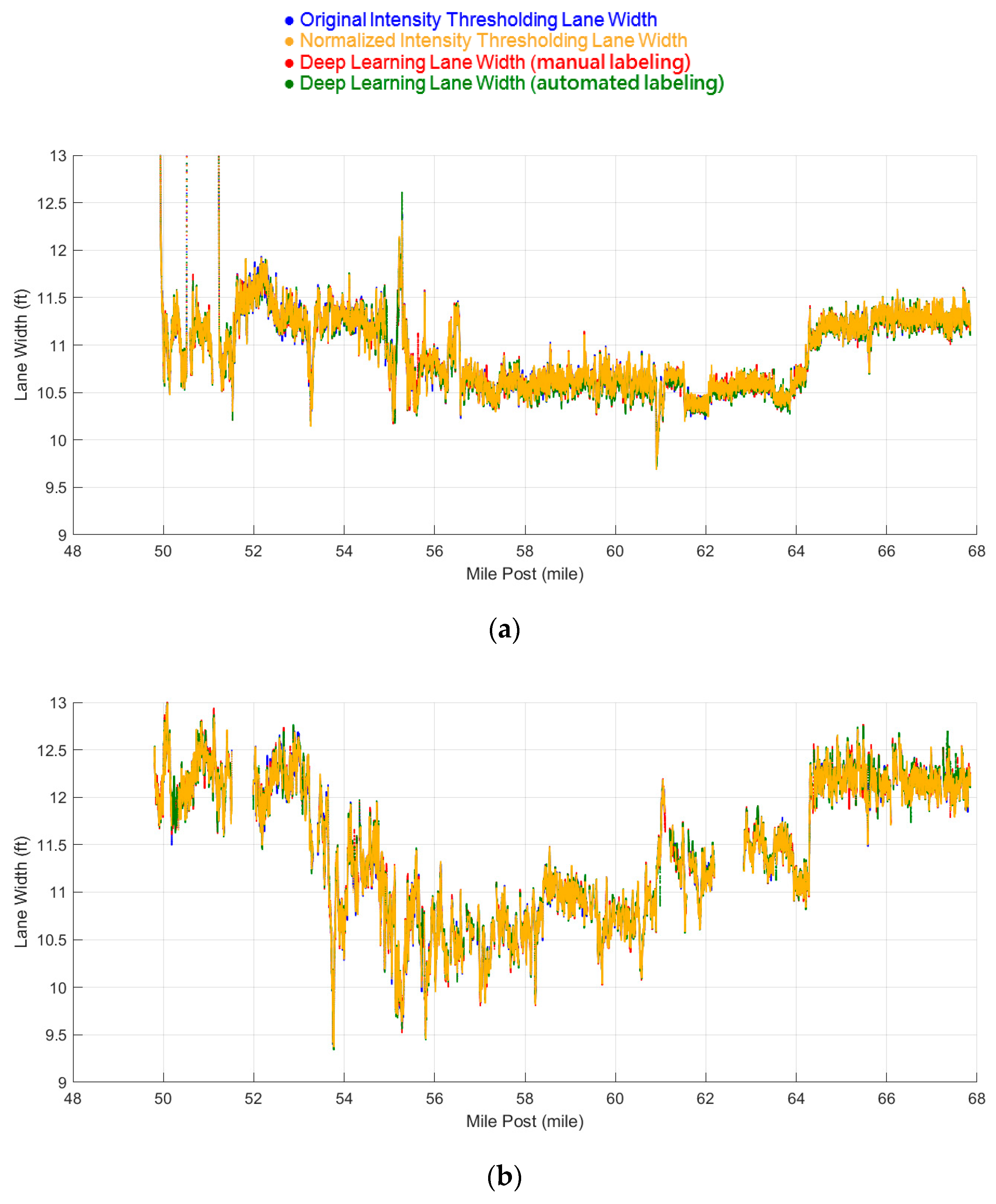
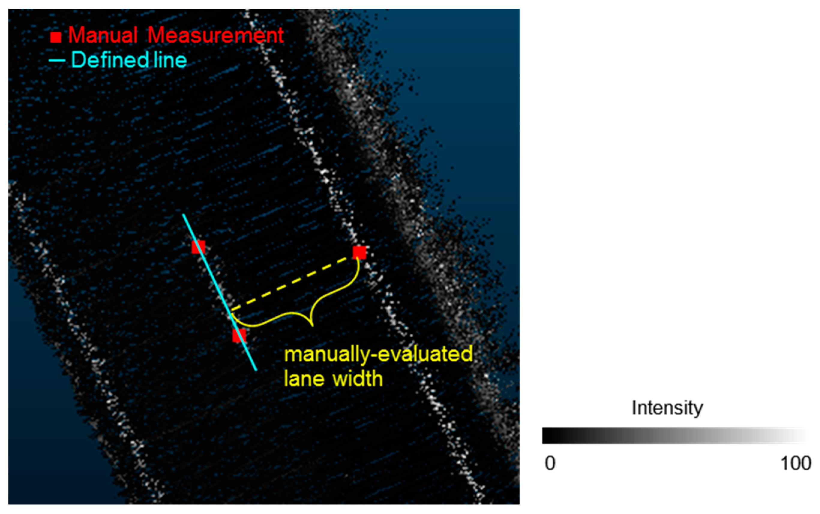
• As a further evaluation of the performance of different lane marking extraction strategies, lane width estimates are derived for each strategy across the different datasets. These estimates have been compared to manually derived ones.
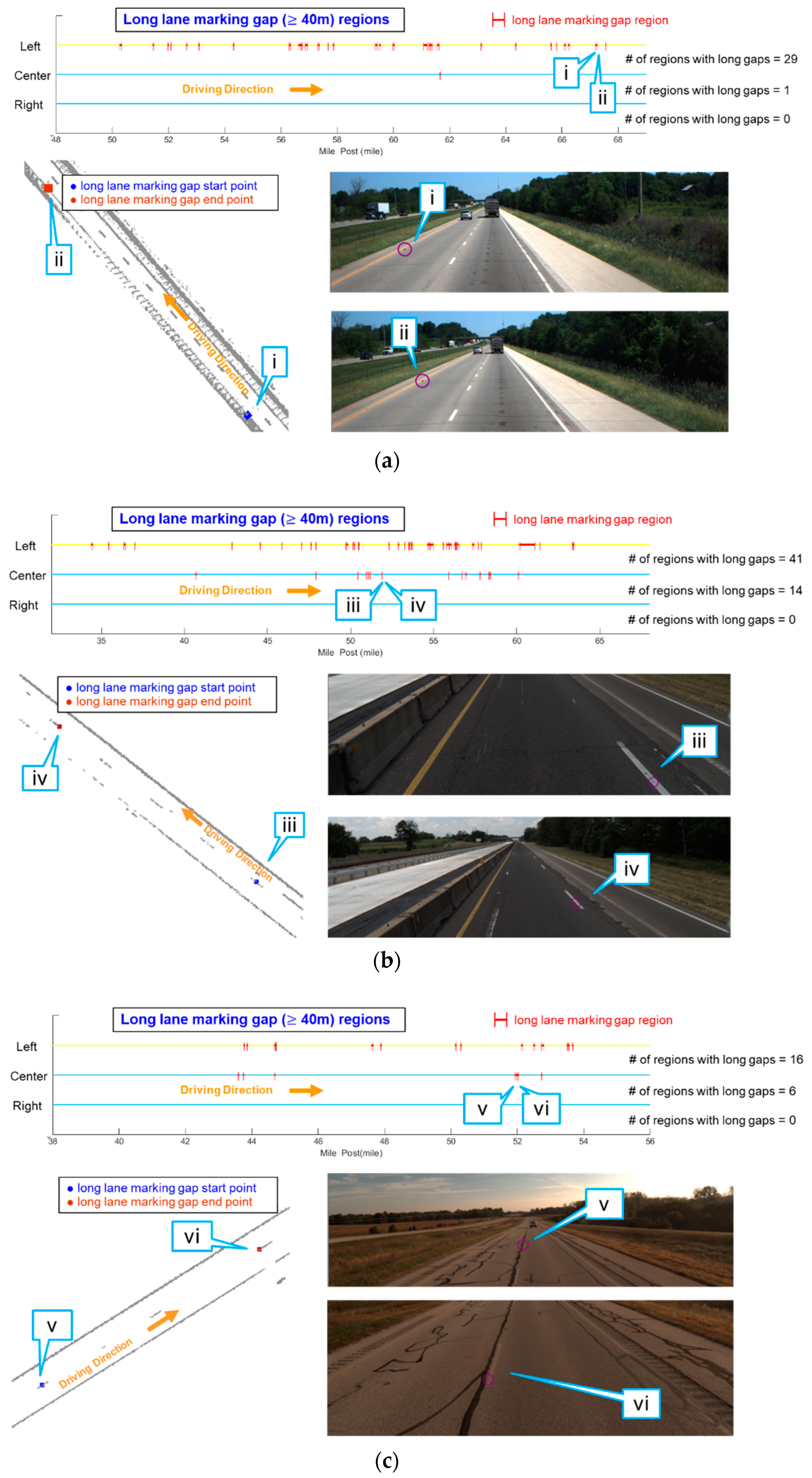
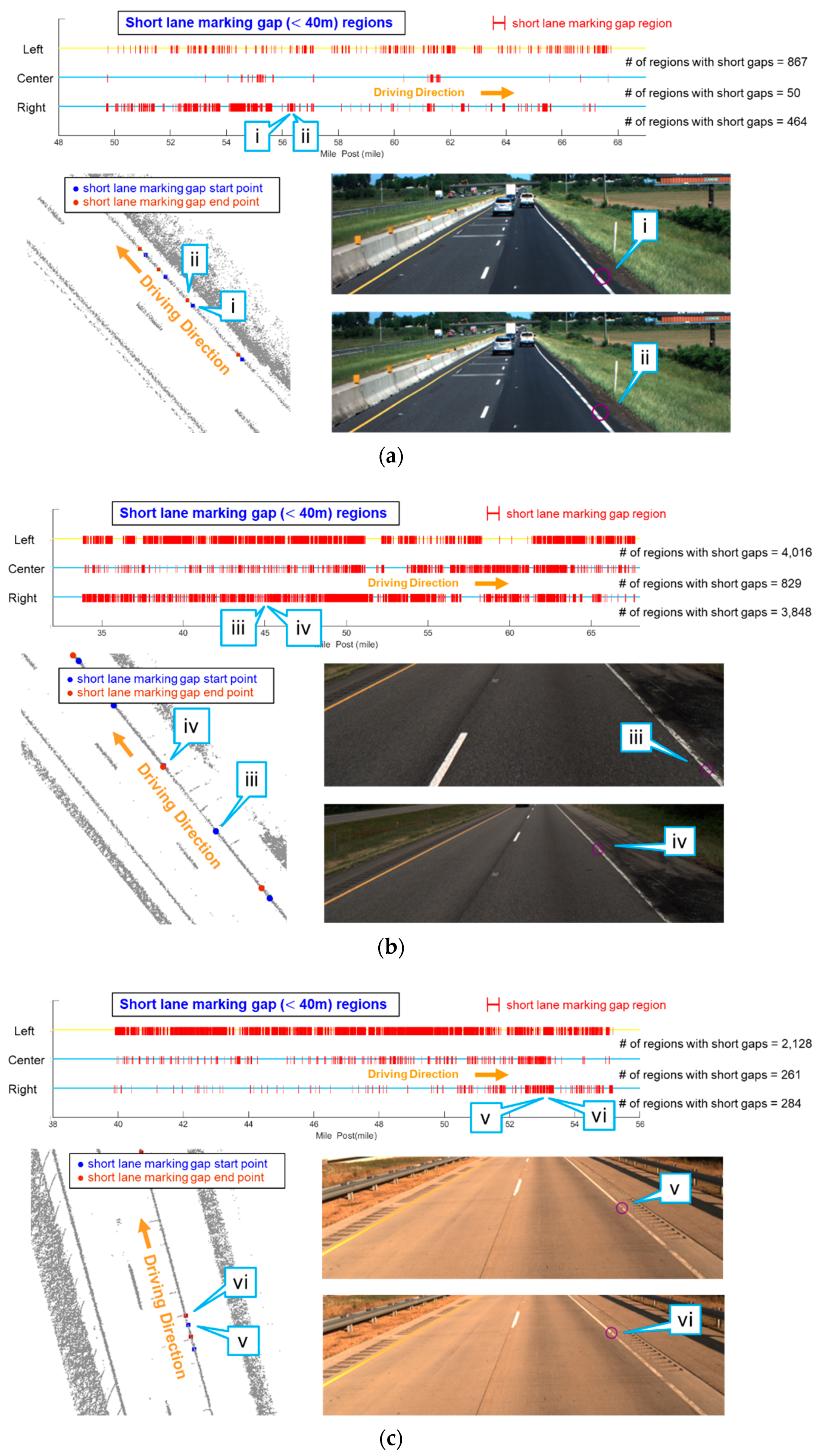
• Derived lane marking from the proposed strategies can be utilized to report lane marking gap regions. This reporting mechanism is quite valuable for departments of transportation (DOT) as it can be used to prioritize maintenance operations and gauge their infrastructure readiness for autonomous driving

The remainder of this paper is organized as follows: Section 2 introduces the LiDAR-based MMS used in this research. Section 3 describes the LiDAR-based MMS point cloud data collected from different test sites. Then, the four lane marking extraction strategies, lane width estimation procedure, and lane marking gap reporting algorithm are described in Section 4, followed by Section 5 that discusses the lane marking extraction results and subsequent lane width estimation. Finally, concluding remarks regarding the different strategies and potential directions for future research are summarized in Section 6.

2. Mobile LiDAR System Used in This Research

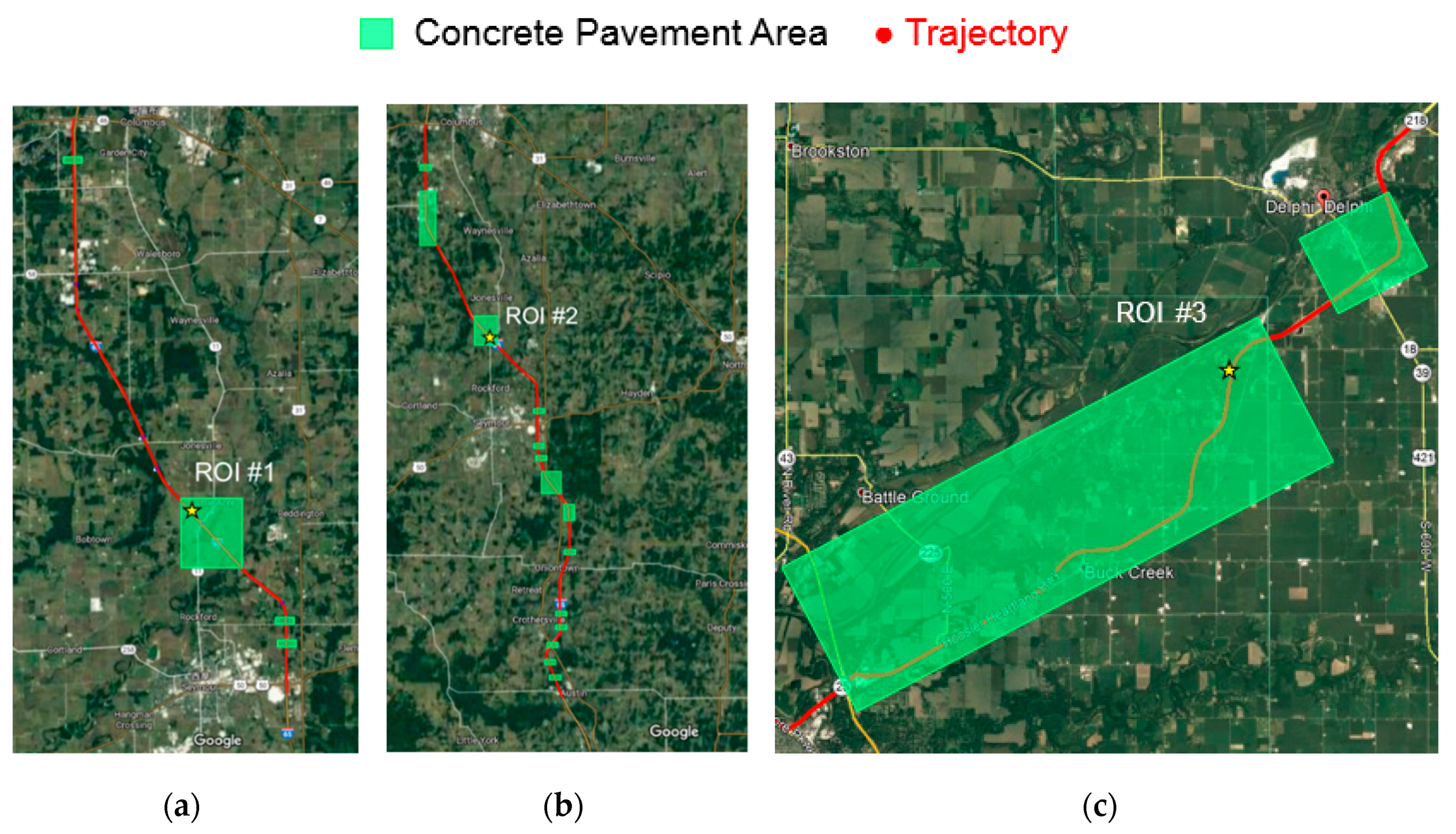
The 3D point cloud datasets used in this research were captured by a wheel-based MMS—Purdue Wheel-based Mobile Mapping System-High Accuracy (PWMMS-HA). Four 3D LiDAR scanners are mounted on the PWMMS-HA (as shown in Figure 1): three Velodyne HDL-32E and one Velodyne VLP-16 Puck Hi-Res. The HDL-32E scanner has 32 radially oriented laser rangefinders that are aligned vertically from +10.67° to –30.67° making up a total vertical field of view (FOV) of 41.34°. The HDL-32E can capture around 700,000 points per second with a maximum range of 100 m (at an accuracy of ± 2 cm) [19]. The VLP-16 scanner, on the other hand, consists of 16 radially oriented laser rangefinders from −10° to +10° (i.e., 20° vertical FOV). The VLP-16 can capture around 300,000 points per second with a maximum range of 100 m (at an accuracy of ± 3 cm) [20]. All four LiDAR scanners can rotate to achieve a 360° horizontal FOV. In addition, three FLIR Grasshopper3 9.1MP GigE cameras (two forward-facing and one rear-facing) are also mounted on the PWMMS-HA. All the cameras are synchronized to capture RGB imagery with a maximum resolution of 9.1 MP at a rate of 1 frame per second per camera. The LiDAR and imaging sensors are georeferenced by an Applanix Position and Orientation System for Land Vehicles (POSLV) 220 Global Navigation Satellite System (GNSS)/Inertial Measurement Unit (IMU) navigation system. The GNSS collection rate is 20 Hz, and the IMU measurement rate is 200 Hz. After GNSS/inertial navigation system (INS) post-processing, the attitude accuracy is ±0.020°, and the positional accuracy is ±2 cm [21]. The expected accuracy of the derived point cloud while considering the LiDAR and navigation system specifications is roughly 2–4 cm at a range of 30 m. This accuracy is estimated using the LiDAR Error Propagation calculator developed by Habib et al. [22].

In order to reconstruct geo-referenced and well-registered point clouds from the different LiDAR scanners, a system calibration procedure [23] is used for estimating the mounting parameters between the onboard LiDAR scanners and GNSS/IMU unit. Another simultaneous LiDAR-camera calibration [24] is also conducted to estimate the mounting parameters of the onboard cameras for the registration of LiDAR point clouds with imagery. Thus, forward and backward projection between the reconstructed point cloud and RGB imagery can be established using the estimated cameras’ mounting parameters and trajectory information. This projection will facilitate the analysis of the performance of the different lane marking extraction strategies. Just as an example, Figure 2 illustrates corresponding image and LiDAR point cloud where the red dot in the latter is projected onto the corresponding image (displayed as an empty magenta circle). Hereafter, a red dot will be used to represent a location in the LiDAR point cloud, while an empty magenta circle will be used to show the same location in RGB imagery.

3. Datasets

Three datasets are utilized in this research to evaluate the performance of different lane marking extraction strategies. These datasets were acquired over two highways (the first two on an interstate highway with the third one covering rural highway). The collection date, used sensor, length, average local point spacing (LPS) [25], average driving speeds, and main pavement type of each dataset are listed in

Table 2. Description of the three LiDAR-based mobile mapping systems (MMS) point clouds.

Road Segment	Collection Date	Used Sensors	Length	Average LPS	Average Speed	Pavement
Dataset 1	2018/05/24	HDL32E-F 1 HDL32E-L 1 HDL32E-R 1	18.04 mile	3.11 cm	45.62 mph	Asphalt mainly
Dataset 2	2019/07/19	HDL32E-F 1 HDL32E-L 1 HDL32E-R 1 VLP16	33.87 mile	3.19 cm	47.42 mph	Asphalt mainly
Dataset 3	2019/10/05	HDL32E-F 1 HDL32E-L 1 HDL32E-R 1 VLP16	15.29 mile	3.16 cm	47.70 mph	Concrete mainly

¹ HDL32E-F, HDL32E-L, and HDL32E-R denote different LiDAR sensors of the same model. LPS = local point spacing.

. The datasets include both concrete pavement and asphalt pavement areas. In dataset 1, as shown in Figure 3a, approximately 2.49 mile-long point cloud was collected along concrete pavement area, and 15.55 mile-long point cloud was collected in asphalt pavement area. For dataset 2, as shown in Figure 3b, around 6.28 of the total 33.87 mile-long point cloud covers concrete pavement area. Finally, only 2.23 of the total 15.29 mile-long point cloud in dataset 3 was collected in asphalt pavement area, as shown in Figure 3c.

4. Methodology

The proposed framework for lane marking extraction is illustrated in Figure 4. First, the road surface is identified from the LiDAR point cloud. Lane markings are directly extracted from the road surface point cloud using the original and normalized intensity thresholding strategies. For the two deep learning approaches, the road surface point cloud is rasterized into intensity images. Two U-net models are trained on manually established and automatically generated labels. The automatically generated labels are based on lane markings extracted through the normalized intensity thresholding strategy. For evaluating the performance of different strategies, obtained lane markings are compared with manually labeled ones. In addition, the extracted lane markings are utilized to derive lane width estimates using an adapted strategy of the one proposed by Ravi et al. [18]. As a further quantitative evaluation, these lane width estimates are also compared to manually derived values. Finally, the lane markings are also analyzed for reporting lane marking gaps.

4.1. Lane Marking Extraction Approaches

In this section, different lane marking extraction strategies are described. We collectively refer to the original and normalized intensity thresholding strategies as “intensity thresholding approaches.” The deep learning strategies using manually derived and automatically established labels are denoted as “deep learning approaches.” As mentioned earlier, the lane marking extraction procedure starts with the identification of the point cloud pertaining to the road surface. In this research, the road surface identification is based on the GNSS/INS trajectory as well as a rough estimate of the IMU height above the road surface. For more details regarding this procedure, interested readers can refer to Ravi et al. [18].

4.1.1. Intensity Thresholding Approaches

Original Intensity Thresholding Strategy

Using the original intensity values, one can use a single threshold (Th_I)—e.g., the one defined by 5th percentile intensity value [18]—to extract hypothesized lane markings from the road surface point cloud, as shown in Figure 5. However, in concrete pavement area, simple thresholding would result in hypothesized lane markings with significant false positives (hereafter referred to as “noise”). This scenario is shown in Figure 6 where more noise is observed since lane markings and pavements have similar high-intensity values in concrete pavement regions. Therefore, such low intensity contrast will negatively affect the performance of a simple thresholding strategy.

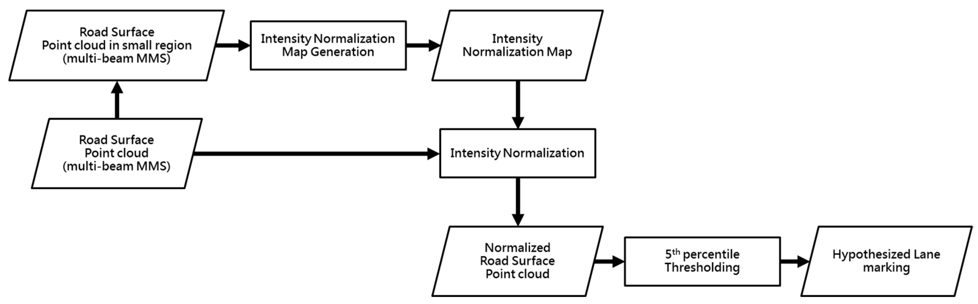
Normalized Intensity Thresholding Strategy

In order to solve the low contrast issue, which is more pronounced in concrete pavement area, this research adopts an intensity normalization strategy for an MMS with one or more multi-beam LiDAR scanners. The normalization process is based on the assumption that intensity values across laser beams should be similar for the same objects [26,27]. In this strategy, the normalized counterpart of an intensity value observed by a particular beam is the conditional expectation of intensity readings by other beams for the same areas where that beam observed the given intensity value. This normalization is applied to each multi-beam LiDAR scanner mounted on the MMS to obtain corresponding normalized intensity values of all laser beams for that scanner. Figure 7 illustrates an overview of the normalized intensity thresholding strategy for a multi-beam LiDAR-based MMS.

First, for a given dataset, a small section is randomly chosen from the road surface point cloud captured by the MMS for the intensity normalization map generation. In case that the small point cloud is captured by more than one scanner, the LiDAR data should be split according to the used scanner. Subsequently, the intensity normalization approach proposed by Levinson and Thrun [26,27] is applied to the small road surface point cloud from each LiDAR scanner. The adopted approach proceeds according to the following steps:

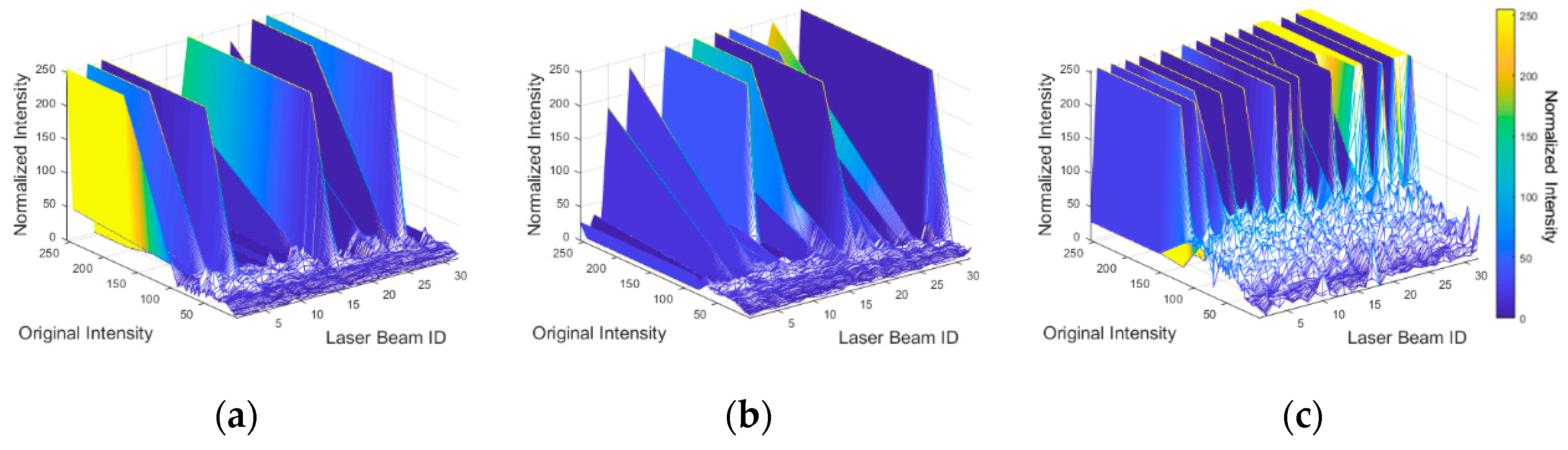
• The small road surface point cloud is gridded into cells. Each cell stores the list of points that lie within its bounding box. For each point, only the intensity value and laser beam ID are stored.
• In order to compute the normalized intensity value of a laser beam j that recorded an intensity value a, we seek all cells that contain the pair (j, a) in the raster grid. The average intensity is computed over these cells while excluding intensity values recorded by laser beam j. The normalized intensity of (j, a) is the resulting average. The original and normalized intensity values are stored in a lookup table (LUT) for the scanner/dataset in question.
• For the intensity values that are not observed in the small road surface point cloud, their normalized counterpart can be calculated by interpolation, using the normalized values associated with the observed intensities.

One should note that, in this research, the small road surface point cloud is randomly selected in concrete pavement area, which exhibits higher minimum and maximum intensity values. Using asphalt pavement regions, with the majority of the intensity values of lower magnitude, might map high-intensity values of both lane markings and concrete pavements to a similar value. This defeats the purpose of increasing intensity contrast between lane markings and pavement surface. In addition, it is assumed that the map generated from the small road surface point cloud of concrete pavements would not negatively affect the intensity contrast between lane markings and asphalt pavement. The performance metrics for lane marking extraction in dataset 2 (asphalt dominant) further validate this assumption, as will be reported in Section 5.1.2.

The choice of the cell size for generating the intensity normalization map was not addressed by Levinson and Thrun [26,27]. The cell size plays a key role—i.e., large cell size might cause more than one type of object surface being located in a single cell, while within a small cell, the laser beams could be too sparse for evaluating a reliable average intensity value. In this research, the cell size is based on the LPS of the point cloud [25]. Prior to intensity normalization, the LPS is evaluated for the small road surface point cloud captured by each scanner. The cell size is determined using a multiplication factor threshold (Th_MF) of the respective LPSs. Since a change in the driving speed from one dataset to another could lead to differences in LPSs, the intensity normalization maps should be generated for each dataset. The intensity values captured by a given scanner are then normalized using the respective LUT for the dataset in question. Finally, hypothesized lane markings can be extracted from the normalized road surface point cloud using the 5th percentile intensity threshold.

4.1.2. Deep Learning Approaches

In this research, two U-net models [17] are trained using manually established and automatically-generated labels. Figure 8 illustrates an overview of the proposed deep learning-based lane marking extraction and U-net model training framework. The first step in this process is to generate intensity images through a 3D-to-2D mapping process. Extracting lane markings from the intensity images is a binary classification task where each pixel is labeled as either belonging to a lane marking or not. This classification task is performed by training a U-net model to identify lane marking pixels in the intensity images. The following subsections describe intensity image generation and labeling, U-net model training, and refinement of U-net predictions.

Intensity Image Generation and Labeling

For generating an intensity image, it is crucial to choose a cell size that can maintain the lane marking details in the derived image as well as reduce computations. The cell size selection should consider both the width of mapped roads as well as the LPS of available data. The width of surveyed highway roads in this research ranges from 12 to 16 m in different regions of the three datasets (i.e., covering two-lane highways including shoulder width). Therefore, the road surface point cloud is partitioned into blocks of length 12.8 m along the driving direction—Figure 9. Further, the LPS analysis of the datasets suggests a point density equivalent to a cell size of approximately 5 cm. Therefore, an image size fixed at 256 × 256 (for U-net input), with a 5 cm cell size, ensures minimal resizing along the length and width of the block while maintaining the level of detail in the point cloud. After partitioning, an intensity enhancement is applied to each point cloud block by choosing a threshold (Th_EN)—e.g., 5^th intensity percentile. Intensity values greater than this threshold are set to 255, while lower intensity values are maintained.

When generating intensity images, the pixel values are derived from the enhanced intensity within the point cloud block. For each cell, its pixel value is defined by taking an average of the intensity values of points falling in it. A second level of enhancement is applied to the generated intensity images—e.g., using a 5th intensity percentile threshold. The two-step enhancement (in the point cloud block and intensity image) helps in amplifying the pixel values corresponding to lane markings and facilitates easier inference from the intensity image by the U-net model. For the following discussion, we hereafter refer to the enhanced image as an “intensity image.” An original road surface point cloud and corresponding intensity image are shown in Figure 10. For U-net training, some intensity images are utilized to establish labels manually for the first U-net model (referred to as “U-net model 1” in Figure 8). For the second U-net model (referred to as “U-net model 2” in Figure 8), labels are generated automatically using lane markings obtained from the normalized intensity thresholding after noise removal according to the following steps:

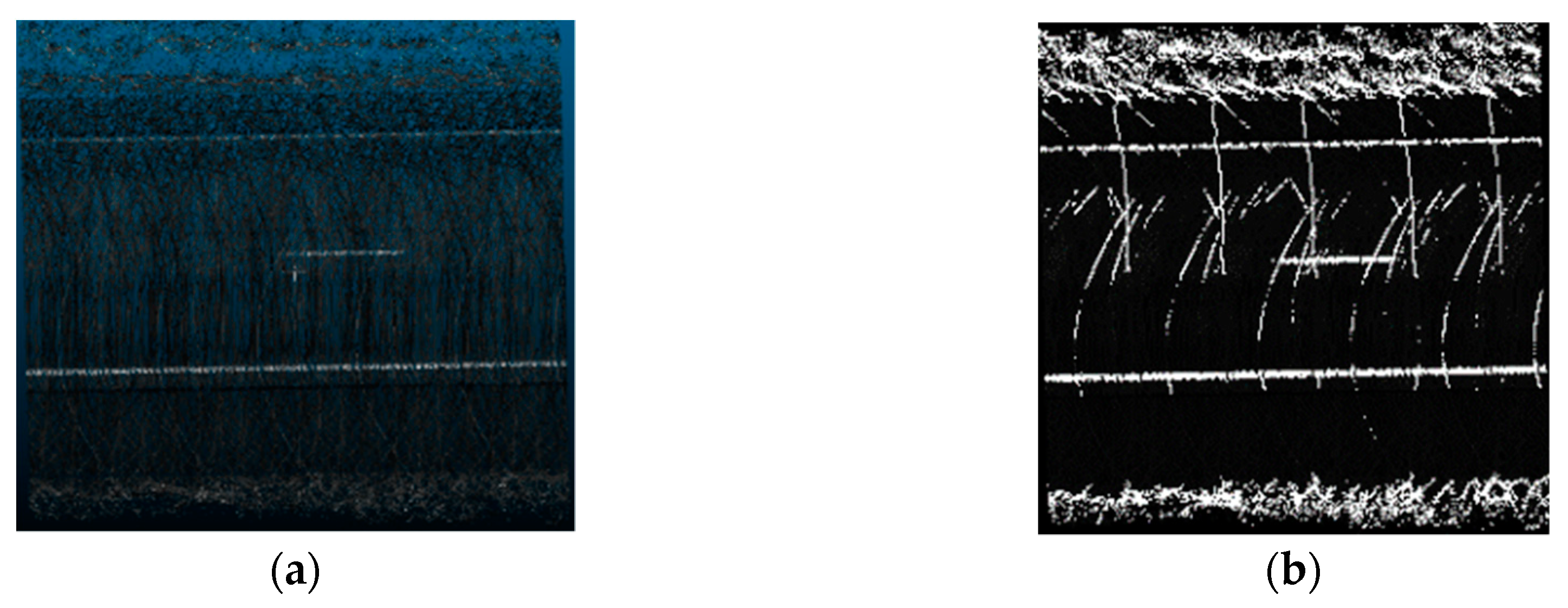
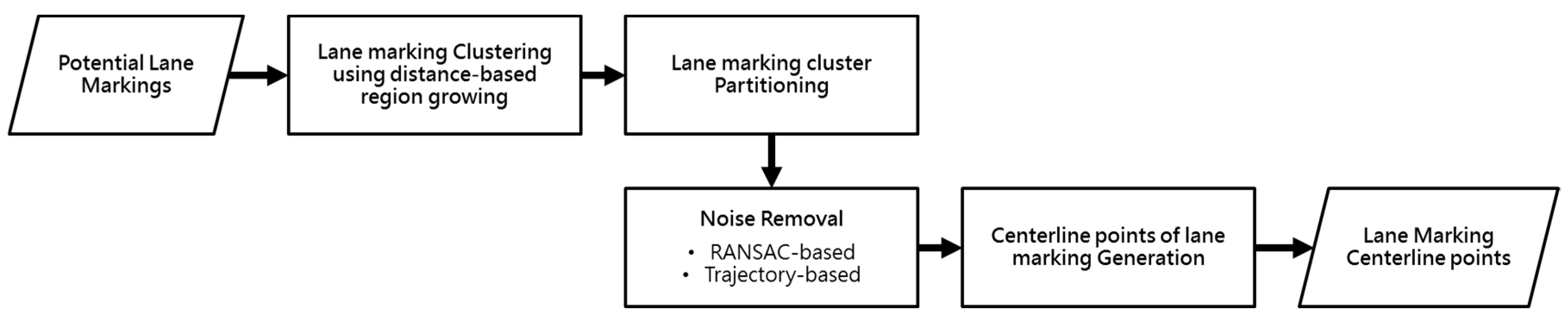
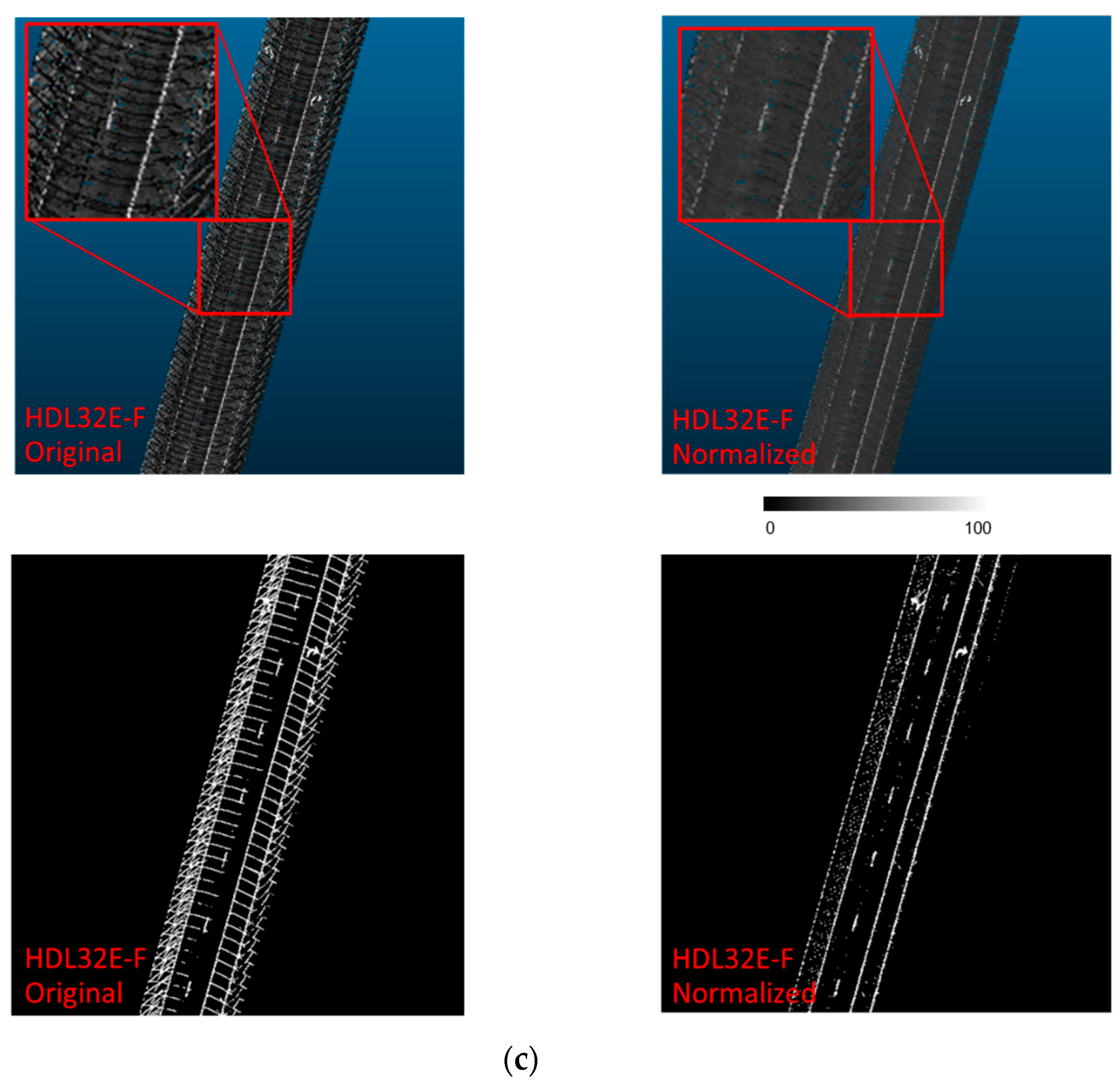
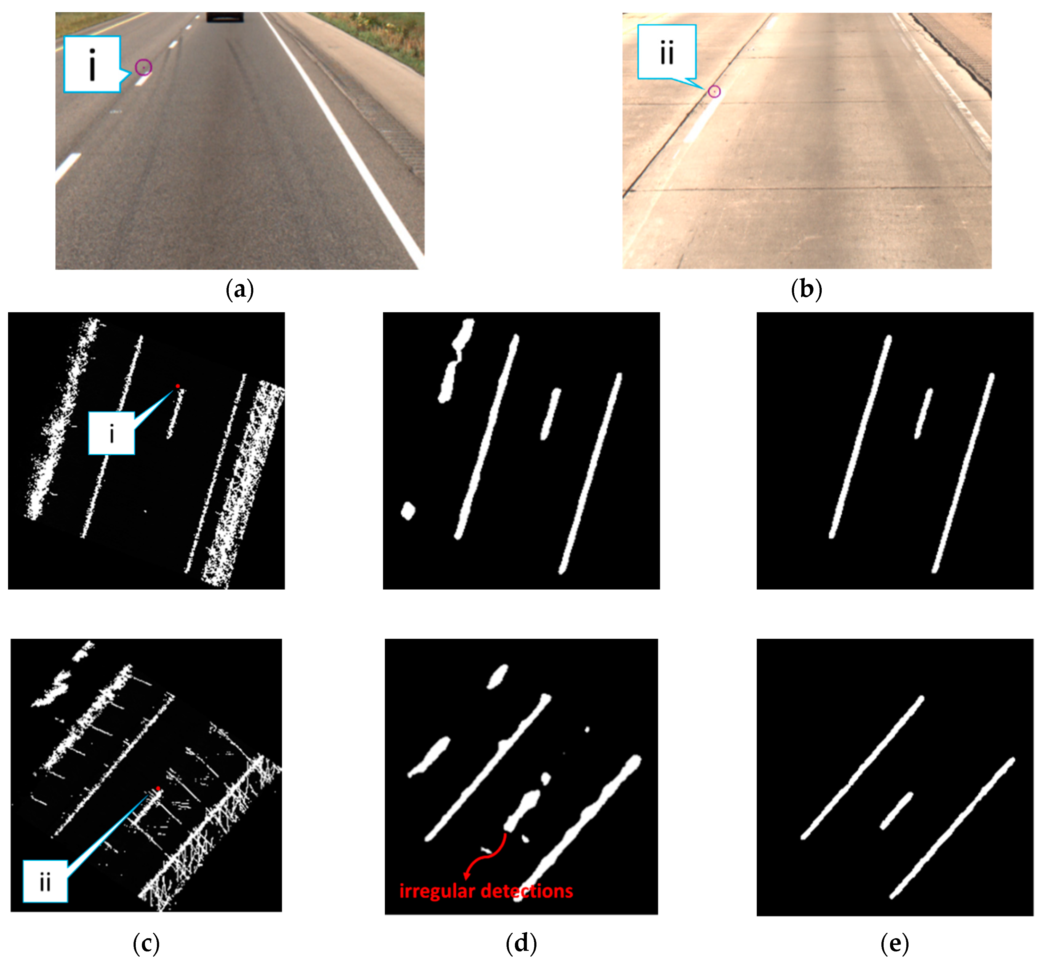
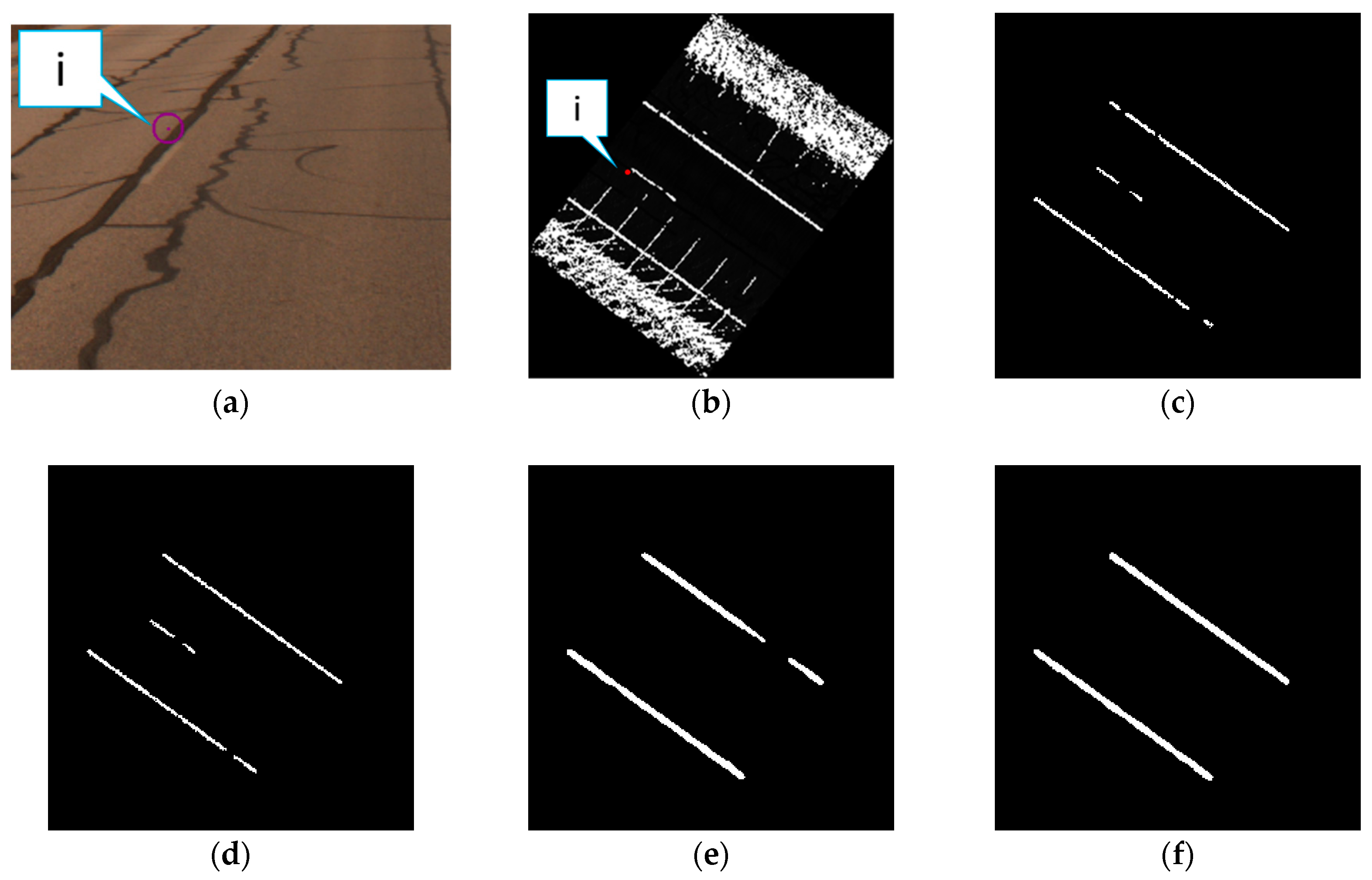
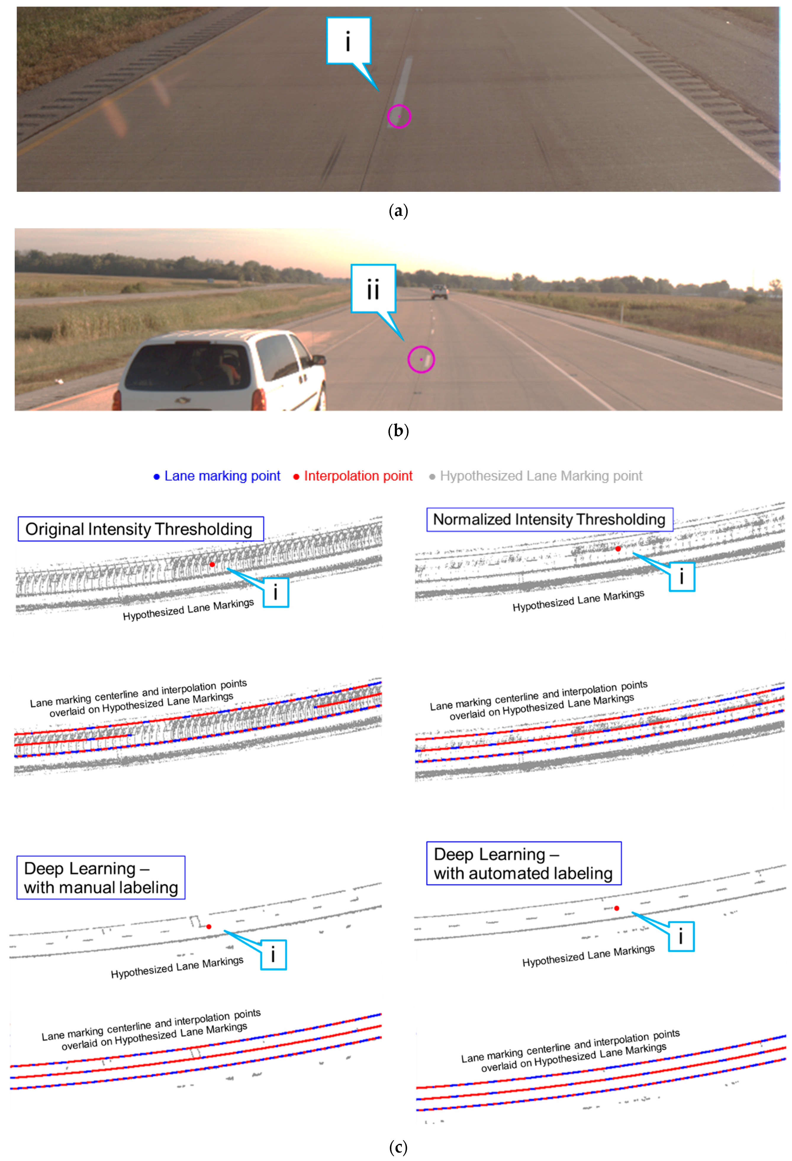
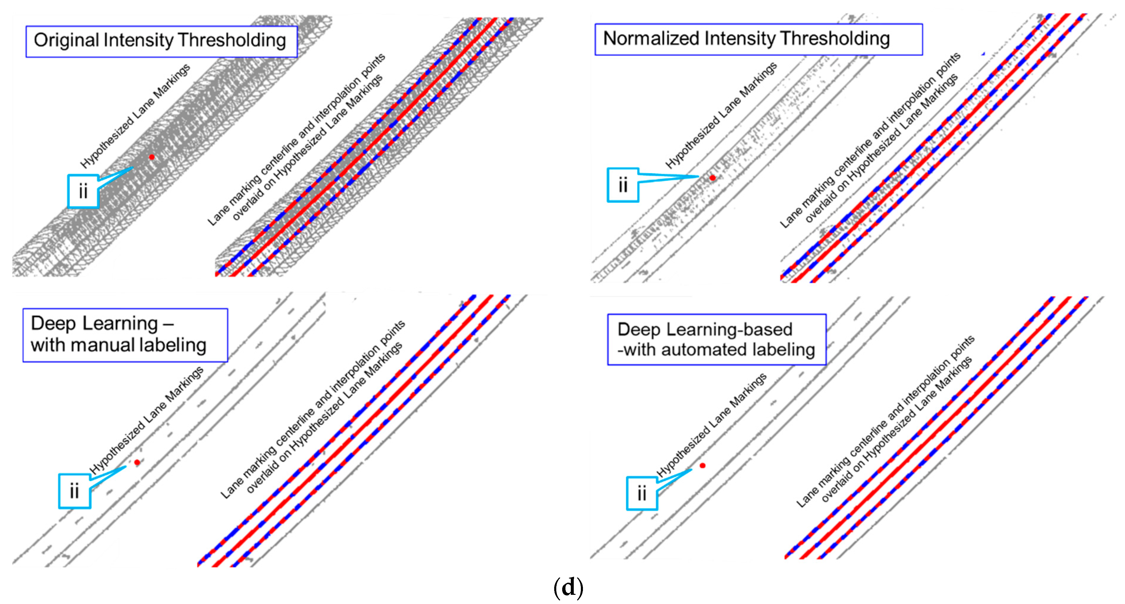
• The noise removal strategy proposed by Ravi et al. [18] (the details of which are described in Section 4.2) is applied to the hypothesized lane markings. Figure 11a,b illustrate the outcome from the normalized intensity thresholding strategy before and after noise removal.
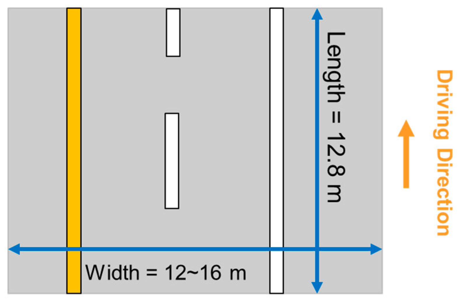
• The point cloud after noise removal, as shown in Figure 11b, is then divided into 12.8 m-long blocks for converting into images with a pixel size and image size of 5cm and 256 × 256, respectively.
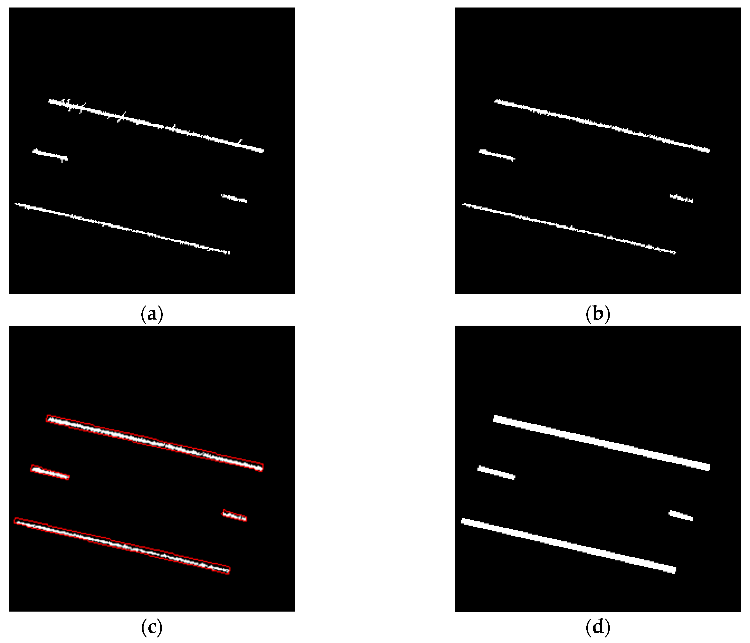
• To ensure better spatial structure for the markings, a bounding box is created around each lane marking in the resulting intensity image, as shown in Figure 11c. Thereafter, all pixels falling within the bounding box are labeled as lane marking pixels. The resultant image, as shown in Figure 11d, serves as a labeled image for the training of U-net model 2.

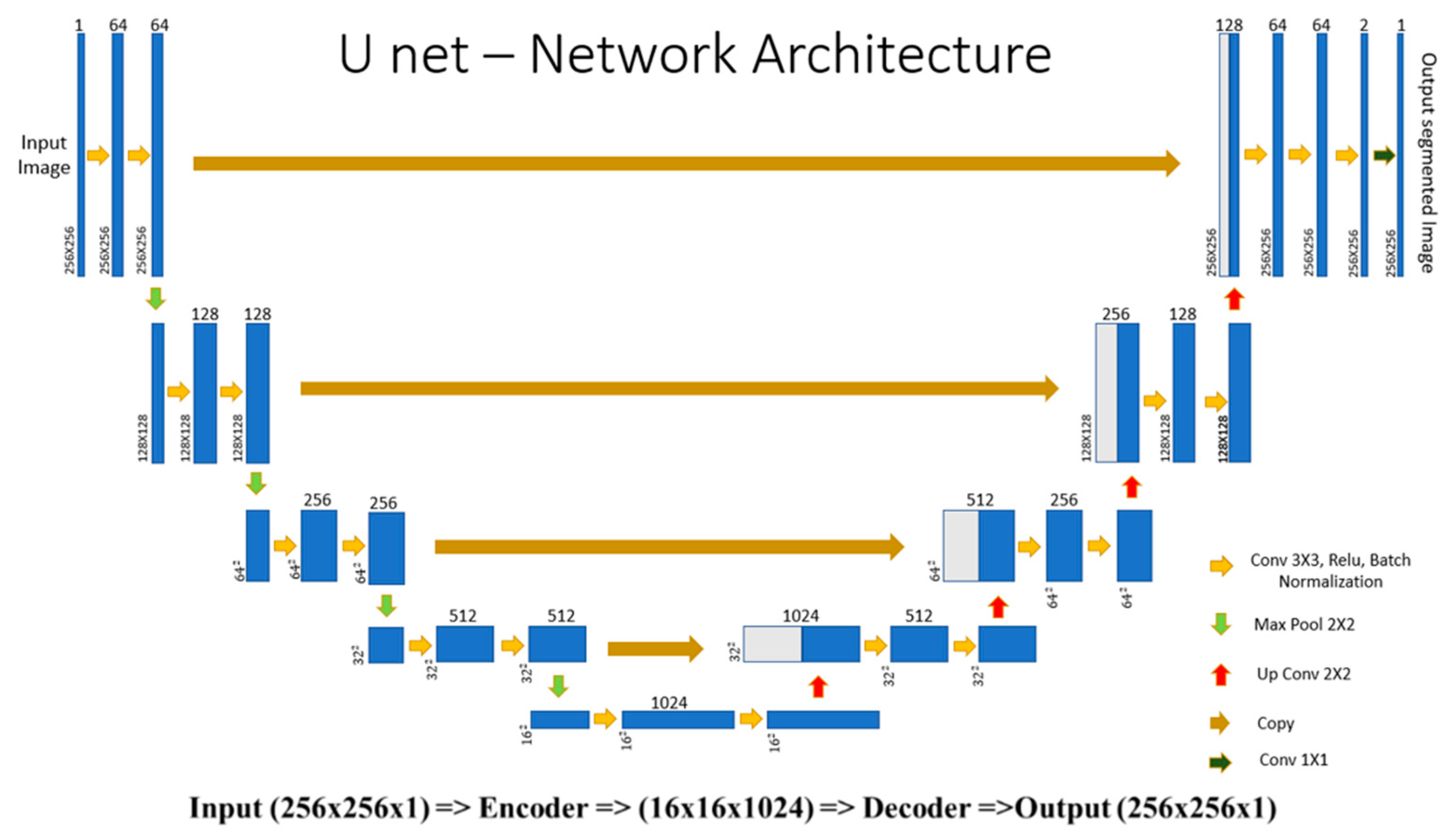
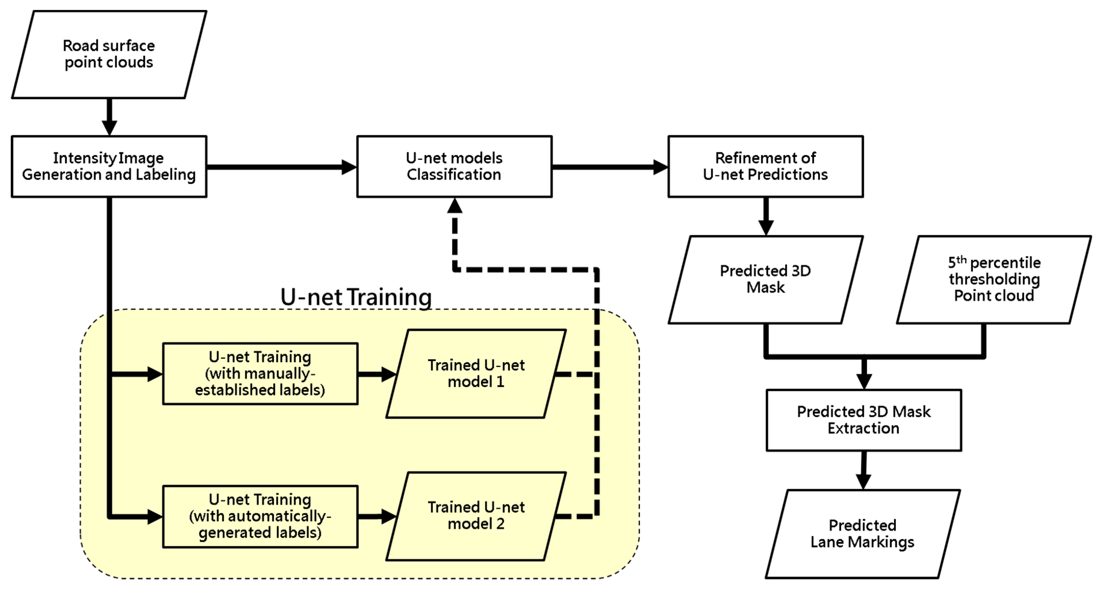
U-Net Model Training

U-net is a fully CNN proposed by Ronneberger et al. [17] for biomedical image segmentation. The adopted network architecture is shown in Figure 12. In our implementation, batch normalization [28] is incorporated since it helps the U-net model to train faster by reducing the internal covariate shift and allowing higher learning rates. Considering the disparity in the number of pixels between lane marking and non-lane marking classes, this research chose a loss function based on the dice coefficient, which measures the degree of overlap between two classes. The dice coefficient [29] is defined as in Equation (1), where y_true and y_pred represent the ground truth and predicted pixels for the lane markings. Each pixel takes a value of either 0 or 1 depending on whether it belongs to non-lane marking or lane marking class, respectively. The dice coefficient value ranges from 0 to 1, where perfect overlap gives a value of 1. Minimizing this loss function leads to the maximization of the Dice coefficient and hence the degree of overlap between the ground truth and predicted lane markings. In order to evaluate the performance of all strategies, precision, recall, and F1-score—represented by Equations (2)–(4) where TP, FP, and FN are the true positives, false positives, and false negatives, respectively—are used. Precision signifies how accurate the positive predictions are whereas recall indicates how well the true lane markings are detected. F1-score, which is used to quantify the overall performance, is a harmonic mean of precision and recall.

$$Dice coefficient=\frac{2{\sum }_{pixels}{\gamma }_{true}{\gamma }_{pred}}{{\sum }_{pixels}{\gamma }_{true}+{\sum }_{pixels}{\gamma }_{pred}}$$

(1)

$$Precision=\frac{\mathrm{TP}}{TP+FP}$$

(2)

$$Recall=\frac{\mathrm{TP}}{\mathrm{TP}+\mathrm{FN}}$$

(3)

$$F_1-\mathrm{score}=2\times \frac{\mathrm{Precision}\times \mathrm{Recall}}{Precision+Recall}$$

(4)

Refinement of U-Net Predictions

After detection by the trained U-net model, predicted 2D lane marking images are projected back to 3D to derive lane marking points. Due to the raster nature of the images, the derived 3D points will be regularly spaced at a 5 cm interval. In order to derive lane markings with a point density similar to that of the original road surface point cloud, the back-projected 3D points are used to generate 2D masks. First, a square buffer cell with a 5cm side length is created around each projected point along the XY-plane. All neighboring cells are then merged to form mask regions, as shown in Figure 13a. As a refinement of the predicted lane markings, mask regions with areas smaller than a pre-defined threshold (Th_area) are removed. The value of Th_area is based on the cell size of the intensity image and minimum area of a dash lane marking. Finally, the original points—whose intensity is within the 5th percentile intensity value—falling within the remaining mask regions are extracted as the final lane marking predictions, as shown in Figure 13b,c.

4.2. Lane Width Estimation Approach

To evaluate the performance of various lane marking extraction strategies, the lane width estimation approach proposed by Ravi et al. [18] is used after its adaptation to handle derived lane markings from intensity thresholding and deep learning strategies. Since predicted markings using either intensity thresholding or deep learning strategies might have false positives, these lane markings should be manipulated to produce their centerline points while removing potential outliers. The used strategy has four main steps, shown in Figure 14: (1) clustering lane markings through a distance-based region growing, (2) partitioning lane marking clusters, (3) noise removal, and (4) generating centerline points for each lane marking cluster. An example illustrating the different steps is shown in Figure 15.

First, a distance-based region growing is applied to the hypothesized lane marking points. If the distance between two lane marking points is less than a distance threshold (Th_dist), they are grouped into the same cluster. This Th_dist is defined based on LPS analysis of the road surface point cloud. After clustering, a minimum point threshold (Th_pt) is used to remove a cluster with fewer points. The Th_pt is determined based on the evaluated LPS and minimum area of a dash lane marking. In this work, Th_pt is only applied to lane marking clusters obtained from the intensity thresholding approaches. For such approaches, the Th_dist and Th_pt thresholds are sequentially used for clustering lane marking points and removing small clusters. For derived lane markings from deep learning approaches, Th_dist is only used for clustering the lane marking points since small area lane marking regions have been already removed through the Th_area threshold during the refinement of the U-net predictions.

Subsequently, all lane marking clusters are partitioned into 3-m-long segments, which is the length of a dash lane marking segment [30]. This partitioning is necessary to represent curved lane markings as polylines. After the partitioning, Random Sample Consensus (RANSAC) and trajectory-based strategies are applied to the lane marking segments for noise removal. First, a best-fitting line for each segment is estimated using the RANSAC algorithm [31]. Based on the fitted line parameters, outlier points within the segment are removed, as shown in Figure 15b. Second, an entire segment which is not parallel to the driving direction is removed, as shown in Figure 15c. Collectively, the RANSAC-based strategy removes outlier points within a hypothesized lane marking segment, while the trajectory-based strategy removes an entire segment that does not represent a lane marking (as indicated by its orientation relative to the system trajectory). Finally, the points in the remaining segments are projected onto the corresponding centerlines.

Once centerline points of the lane markings are generated, the next step is to cluster them into right-side and left-side groups for a given lane, as shown in Figure 16a. The basic concept of the adopted centerline clustering algorithm is to start with a segment at the beginning of a road surface and using its direction as a reference. The reference segment is augmented with the next centerline segment along its direction. The centerline segment, which has been augmented last to a group, is then used to define the new reference direction, and the process is repeated. Then, a linear interpolation is conducted for filling the gap between two successive centerline segments in a given group, as shown in Figure 16b. Two thresholds, defining the minimum and maximum bounds for conducting the interpolation, are used. For the minimum bound, we use Th_dist—which was previously used for the distance-based region growing. Therefore, for clustered centerline points that are farther apart than Th_dist, we carry out linear interpolation between them. To avoid linear interpolation on curved road segments, we define a maximum distance threshold, denoted as Th_miss. For centerline points that are farther apart more than Th_miss, a region of missing lane marking is assumed and reported. In this research, Th_miss is set to 40 m, which is equivalent to the extent of three missing dash lane markings along road surface. One should note that Th_miss is determined based on the minimum radius of curvature for designing highways [32]. With a design speed of 70 mph and chord of length 40 m, the corresponding arc obtained by the minimum curvature (2040 ft) is about 40.01 m. The difference between Th_miss and the corresponding arc is 1 cm, which is within the noise level of the MMS. However, Th_miss should be revised accordingly when the minimum curvature changes due to a decline in design speed on suburban or urban roads.

Table 3. Recommended values of Th_miss at different design speeds.

Design Speed	Minimum Radius of Curvature	Recommended Thmiss	Length of arc
30 mph	231 ft	10 m	10.01 m
40 mph	485 ft	20 m	20.02 m
50 mph	833 ft	25 m	25.01 m
60 mph	1330 ft	35 m	35.01 m
70 mph	2040 ft	40 m	40.01 m

lists the recommended values of Th_miss for adjustment at different design speeds. Finally, all points, including original lane marking centerline points and interpolated points, are down-sampled to space the points at an interval of Th_dist. Thereafter, the down-sampled points from the above steps are utilized for deriving lane width estimates (i.e., a lane width estimate is derived at an interval of Th_dist except in areas with missing lane markings where the center line points on either side of the lane are farther apart than Th_miss).

4.3. Lane Marking Gap Reporting

As mentioned previously in Section 4.2, for lane width estimation, 3-m-long lane marking segments are generated through the strategy proposed by Ravi et al. [18]. Gaps between these segments correspond to areas with worn-out/missing lane markings and/or road intersections. While an interpolation is conducted to fill the gaps for lane width estimation, interpolated segments can be analyzed to provide a report as to whether these gaps are caused by worn-out/missing lane markings or intersections. Moreover, these reported regions and the corresponding RGB imagery visualization can be utilized for lane markings inspection, which could replace in-situ inspection. In this research, lane markings are solely defined based on intensity returns from the road surface (i.e., other highway information is not incorporated to check if a gap is a result of an intersection or low-intensity returns from lane markings). Thus, the gaps between the lane marking segments are categorized into two classes—long lane marking gap regions and short lane marking gap regions. According to the Federal Highway Administration (FHWA) [30], dash lane markings encompass 9-m gaps, and the overall width of a two-lane intersection on highways is designed to be 102–120 ft (31.1–36.6 m). Based on this information, an algorithm is proposed for automatically reporting gaps along lane markings. Starting with the previously generated 3-m-long segments corresponding to the dash and edge lane markings, gaps longer than Th_miss (which is used for avoiding interpolation in Section 4.2 and is slightly larger than the overall width of a two-lane intersection) are identified as long lane marking gap regions. Remaining gaps (less than Th_miss) are reported as short lane marking gap regions based on two cases, as shown in Figure 17: (1) when a gap between consecutive dash lane marking segments is greater than a dash-line gap threshold (Th_dash), as shown in Figure 17a, and (2) when a gap between consecutive edge lane marking segments is greater than the distance threshold (Th_dist) as shown in Figure 17b. Th_dash is defined as 10 m since it is slightly larger than the standard length of a gap between two successive dash lines (9 m), and Th_dist is set to 20 cm, which is used for the distance-based region growing—as discussed in Section 4.2. One should note that the lane marking segments derived from the normalized intensity thresholding strategy and U-net model 2 are used to report lane marking gap areas. More specifically, lane markings extracted from the former are utilized to report gaps along edge lane markings while the results obtained from the latter help in the identification of the gaps along dash lane markings. This framework, based on results that will be illustrated in Section 5.2, ensures that areas with lane marking gaps are not underestimated.

5. Experimental Results and Discussion

In this research, the three datasets were surveyed on two-lane highways (datasets 1 and 2 are on an interstate highway while dataset 3 is on a rural highway). The PWMMS-HA can capture point clouds for both driving and non-driving lanes, hereafter called “lane 1” and “lane 2”, respectively. Road surface point clouds covering lanes 1 and 2 were used for lane marking extraction and lane width estimation. The thresholds used for lane marking extraction through the different strategies, lane width derivation, and reporting lane marking gap regions are shown in

Table 4. Thresholds used for lane marking extraction and lane width derivation.

Threshold	Description	Used for	Value
ThI	Percentile intensity threshold for lane marking extraction from point clouds	Intensity thresholding approaches	5%
ThMF	LPS multiplication factor for cell size definition (generating intensity normalization maps)	Normalized intensity thresholding	4
ThEN	Percentile intensity threshold for intensity enhancement	Deep learning approaches	5%
Thdist	Distance threshold for a distance-based region growing	Lane width estimation approach	20 cm
Thpt	Minimum point threshold for cluster removal (intensity thresholding approaches)	Lane width estimation approach	30 pts
Tharea	Minimum area threshold for 2D mask removal (deep learning approaches)	Lane width estimation approach	50 cm2
Thmiss	Missing lane marking threshold for reporting a missing lane marking region	Lane width estimation approach	40 m
Thdash	Distance threshold for reporting short lane marking gaps of dash lines	Short lane marking gaps reporting	10 m

. The values of these thresholds are kept the same across all datasets.

5.1. Lane Marking Extraction Results

5.1.1. Intensity Thresholding Approaches

In this research, small road surface point clouds in ROIs 1, 2, and 3, as shown in Figure 3, were randomly selected in concrete pavement areas to generate the intensity normalization maps for each dataset. The number of the sensors, driving speeds, and map generation cell sizes of these small point clouds in these ROIs are listed in

Table 5. Data acquisition specifications, extent of point cloud regions, and cell size for HDL32E and VLP16 LiDAR units for intensity normalization map generation for the three datasets.

ROI	1	2	3
Length of Dataset (m)	29,032.57 (18.04 mile)	54,508.48 (33.87 mile)	24,606.87 (15.29 mile)
# of sensors	3	4	4
Mean. speed (mph)	49.39	48.44	64.85
Max. speed (mph)	52.99	59.84	74.58
Min. speed (mph)	45.58	44.38	55.43
Length of ROI (m)	155	190	155
Cell Size of HDL32E sensors (m)	0.12	0.12	0.25
Cell Size of VLP16 sensor (m)	0.20	0.20	0.30

. According to the number of sensors used for the different datasets in Table 5, the total number of the intensity normalization maps generated for datasets 1, 2, and 3 are 3, 4, and 4, respectively. As mentioned previously, a cell size for generating the map is chosen based on the LPS of the small point cloud, which is affected by the driving speed and the number of beams of a LiDAR sensor. Thus, for the same LiDAR sensor, the cell size is relatively large in ROI 3 because of faster driving speed, as shown in Table 5. In addition, for the same ROI, the cell size of VLP16 is slightly larger due to the fewer laser beams.

Just as an example, Figure 18 shows the intensity normalization maps for one of the HDL32E LiDAR units in ROIs 1, 2, and 3. For the same LiDAR unit, samples of road surface point clouds with the original and normalized intensity values, and corresponding hypothesized lane markings in these ROIs are illustrated in Figure 19. As can be seen in Figure 18, the intensity normalization map for ROI 3 is significantly different from those for ROIs 1 and 2. This difference is attributed to the fact that datasets 1 and 2 were acquired on the same interstate highway, while dataset 3 was collected on a rural highway. For interstate highways, pavement material more resistant to wear and tear is used when compared to that for rural highways [33]. As expected, properties of the pavement surface strongly influence the original intensity values of the road point cloud and subsequently the corresponding intensity normalization map. Another evidence supporting the impact of pavement surface on intensity values can be seen in Figure 19, where the original intensity values in ROI 3 are significantly higher than those for ROIs 1 and 2. Once the intensity values of road surface point clouds were normalized, the hypothesized lane markings were extracted using a 5th percentile intensity threshold (Th_I). For performance comparison, the original point cloud was also utilized to extract hypothesized lane markings using the same threshold. It is apparent that hypothesized lane markings with less noise were extracted from the normalized point cloud, as shown in Figure 19.

5.1.2. Evaluation of Different Lane Marking Extraction Strategies

For training the U-net models, a total of 400 manually labeled intensity images and 1183 automatically labeled intensity images are used. Another 104 manually labeled images and 238 automatically labeled images are used for validation—which is part of the training process. The training and validation images are derived from datasets 1 and 3. The training images have been also augmented during each training epoch using: a) rotation of the image in the range from 0° to 180° in a clockwise direction, b) zooming in and out by resizing image between 80% (zoom in) to 120% (zoom out) of its original size, and c) horizontal flip. Additionally, a test dataset of 174 images is also curated from dataset 2 for performance evaluation of both intensity thresholding and deep learning approaches. Specifically, for the former, lane marking point cloud is converted to intensity image for subsequent performance evaluation. The experimental settings for training the U-net models are listed in

Table 6. Experimental settings for training the U-net models.

Experimental Setting	Description	Associated Values
Learning rate	Step size by which gradient of the loss function is scaled to update the network weights	8 × 10−4
Batch size	Number of training examples fed to the network for a single update of the network weights	8
Epoch	One cycle (forward and backward pass) where the network has seen all training examples once constitutes an epoch.	100
Early stopping	The training is stopped when validation loss does not improve from the current lowest value for a certain number of consecutive epochs called patience. This helps in preventing overfitting to training data.	Patience: 15
Decay of learning rate	The learning rate is also decayed by a factor of 10 when validation loss does not improve from the current lowest value for patience number of consecutive epochs.	Patience: 5 Decay factor: 10

. An Adam optimizer is used to update the network’s weights. Finally, the U-net models are trained on the Google Colaboratory platform that provides K80 GPU access. In machine and deep learning applications, a loss value quantifies the difference between ground truth and prediction. A high loss value indicates poor prediction and vice versa. Figure 20 shows the training loss (calculated on training data) and validation loss (calculated on validation data) plots for U-net models 1 and 2. The plots show the loss values at each epoch of the training process (i.e., training and validation loss values are evaluated for each training epoch). While training data helps the model to optimize its weights for the given classification task, it is the performance on validation data that indicates if the model performs well on unseen data. The plots indicate that U-net model 2 achieves the lowest validation loss of 0.118, while model 1 achieves 0.173 loss value. This can be attributed to the larger training samples for U-net model 2, which helps it to learn varied scenarios.

Table 7. Performance metrics for the lane marking extraction strategies in dataset 2.

Lane Marking Extraction Strategies	Precision	Recall	F1-Score
Original intensity thresholding	84.1%	63.5%	72.3%
Normalized intensity thresholding	83.9%	74.4%	78.9%
Deep learning with manual labeling	60.5%	98.9%	75.1%
Deep learning with automated labeling	84.0%	87.9%	85.9%

presents the performance metrics for the state of the art strategies (original intensity thresholding and deep learning with manual labeling) and proposed approaches (normalized intensity thresholding and deep learning with automated labeling).

Comparing the deep learning approaches, U-net model 1 shows high recall but poor precision rate resulting in a low F1-score. This means that false-positive detection for model 1 is significant (i.e., the model cannot distinguish well between lane markings and high-intensity outliers). On the other hand, U-net model 2 shows large, comparable precision and recall values leading to a much higher F1-score than model 1. This better performance can be explained by 2.5 times more training samples in U-net model 2 in comparison to U-net model 1. Larger training data helps U-net model 2 to learn a variety of scenarios and enables it to lower its false-positive rate in comparison to model 1. Samples of original intensity images and corresponding images with predicted lane markings derived from the deep learning strategies are displayed in Figure 21. As far as the shape of the detected lane markings is concerned, U-net model 1 tends to obtain irregular detections, especially when the lane marking is surrounded by high-intensity outliers, as shown in Figure 21d. On the other hand, U-net model 2 is capable of extracting the regular structure of lane markings, as shown in Figure 21e.

Figure 22 and Figure 23 depict samples of original intensity images and corresponding images with predicted lane markings obtained from the four different strategies in yellow edge lane marking and worn-out dash lane marking areas, respectively (both samples are over asphalt pavement). In these figures, one can observe that the deep learning approaches show much higher recall (i.e., most of the true lane markings have been identified), while the intensity thresholding ones show higher precision (i.e., a lower percentage of false positives). This is expected since the lane markings extracted by the intensity thresholding were processed through the noise removal strategy that removes a significant number of lane marking outliers. However, during the noise removal procedure, some true lane markings could be wrongly eliminated, especially for yellow lane markings where point density is low. This results in a lower recall rate for the intensity thresholding approaches. The deep learning approaches, in contrast, can extract lane markings in such cases. This can be explained by the fact that they detect lane markings based on both content and context (intensity as well as point density and location of points), while the intensity thresholding approaches rely on content alone (intensity and point density), as shown in Figure 22. However, the deep learning approaches miss worn-out dash lane markings in some areas, as shown in Figure 23e,f. This is because of the training data bias where the point density of dash lane markings is usually high because of a small scanner-to-object distance for these markings. Since worn-out dash lane markings have low point density, missing detection could be expected from deep learning approaches. One should note that the argument of context does not hold here (contrary to edge lane markings) since dash lane markings have a smaller length. In contrast, the intensity thresholding approaches can extract these lane markings if their properties satisfy the criteria specified by the Th_pt and Th_dist thresholds during the noise removal strategies, as shown in Figure 23c,d. By utilizing the respective shortcomings of the intensity and deep learning approaches in areas of low point density, a conservative estimate of lane marking gap regions is reported along with their locations, which can be visually inspected through RGB imagery. Thus, based on results illustrated in Figure 22 and Figure 23, lane markings from normalized intensity thresholding strategy are analyzed to identify gaps along edge lines while lane markings extracted through U-net model 2 are utilized to report gaps along dash lines in Section 5.3.

5.1.3. Comparison Between Asphalt and Concrete Pavement Areas

In addition to the condition of the lane marking, the nature of the pavement surface plays a critical role in lane marking extraction. As mentioned previously, while asphalt pavements have low reflectivity, concrete pavements produce high-intensity values, which are close to those for lane markings. Figure 24 illustrates typical intensity images for asphalt and concrete pavement regions in dataset 3. Low intensity contrast between lane markings and its surrounding concrete pavement leads to high noise in the original intensity thresholding strategy. For the same regions in Figure 24, the predicted lane marking images derived from all strategies are presented in Figure 25 and Figure 26. In asphalt pavement area, all the strategies lead to complete extraction of lane markings, as shown in Figure 25. However, in concrete pavement area, the original intensity thresholding cannot completely extract edge lane markings, as shown in Figure 26b, but the normalized intensity thresholding strategy and deep learning approaches avoid this problem. These three strategies eliminate high noise in concrete pavement area while extracting all lane markings.

The length of the road segments where lane markings have been extracted are also compared in dataset 3 with dominant concrete pavement. Figure 27 shows the results of the length comparison. As mentioned previously, road surface point clouds covering two-lane highways were used for lane marking extraction. Thus, all the datasets contain dash center lines and solid edge lines on either side of the center dash lines, hereafter respectively called “center, left, and right lane markings,” as shown in Figure 27a. The length of the lane markings (center, left, and right lane markings) obtained from all strategies are evaluated for both asphalt and concrete pavement areas in dataset 3. One should note that in dataset 3, the driving lane was maintained throughout the data collection campaign and was bounded by the center and right lane markings. Dataset 3 is 15.29 mile (24.61 km) long and the total length of the different lane markings extracted in asphalt and concrete pavement areas are tabulated in Figure 27b,c, respectively. As shown in Figure 27b,c, the percentages of the extracted lane markings indicate gaps, which could be caused by, (1) missing/worn-out lane markings and/or road intersections or (2) shortcomings of the strategies themselves. Following are the findings of the analysis:

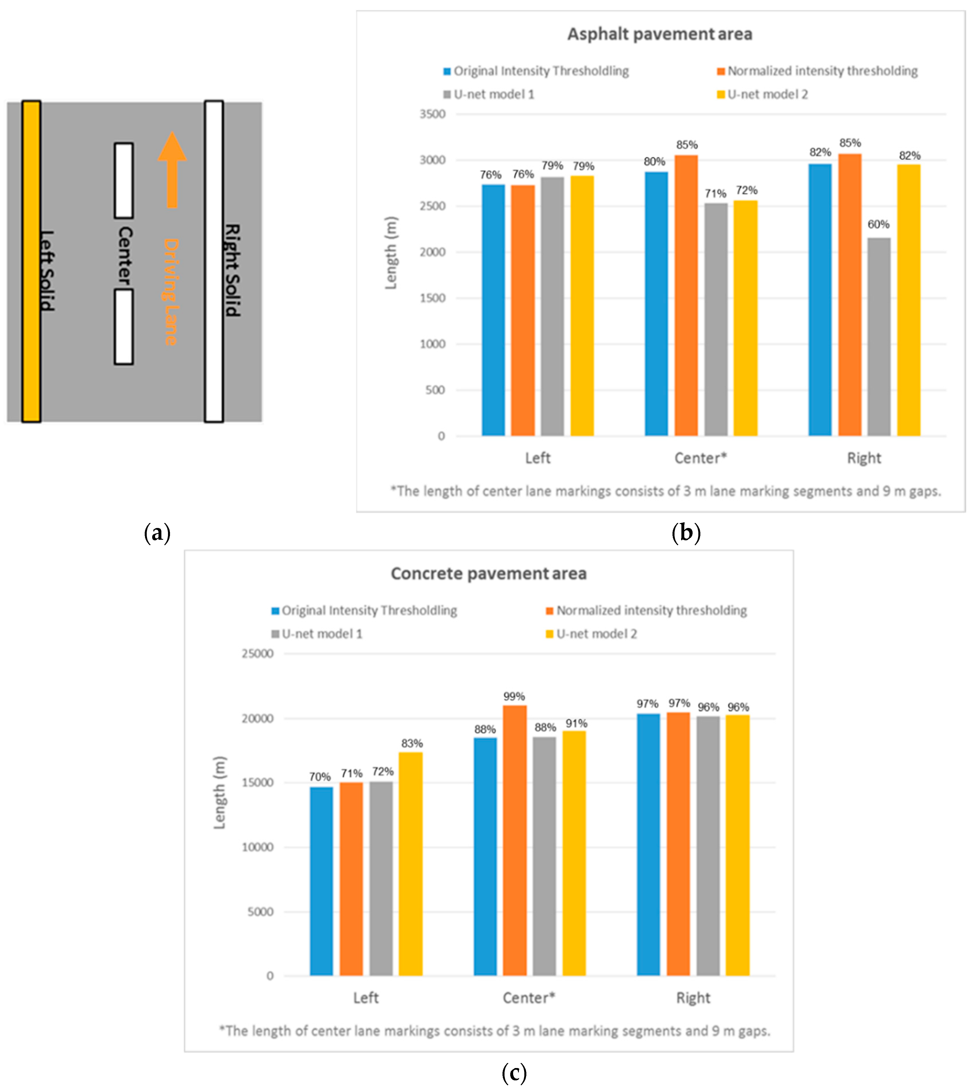
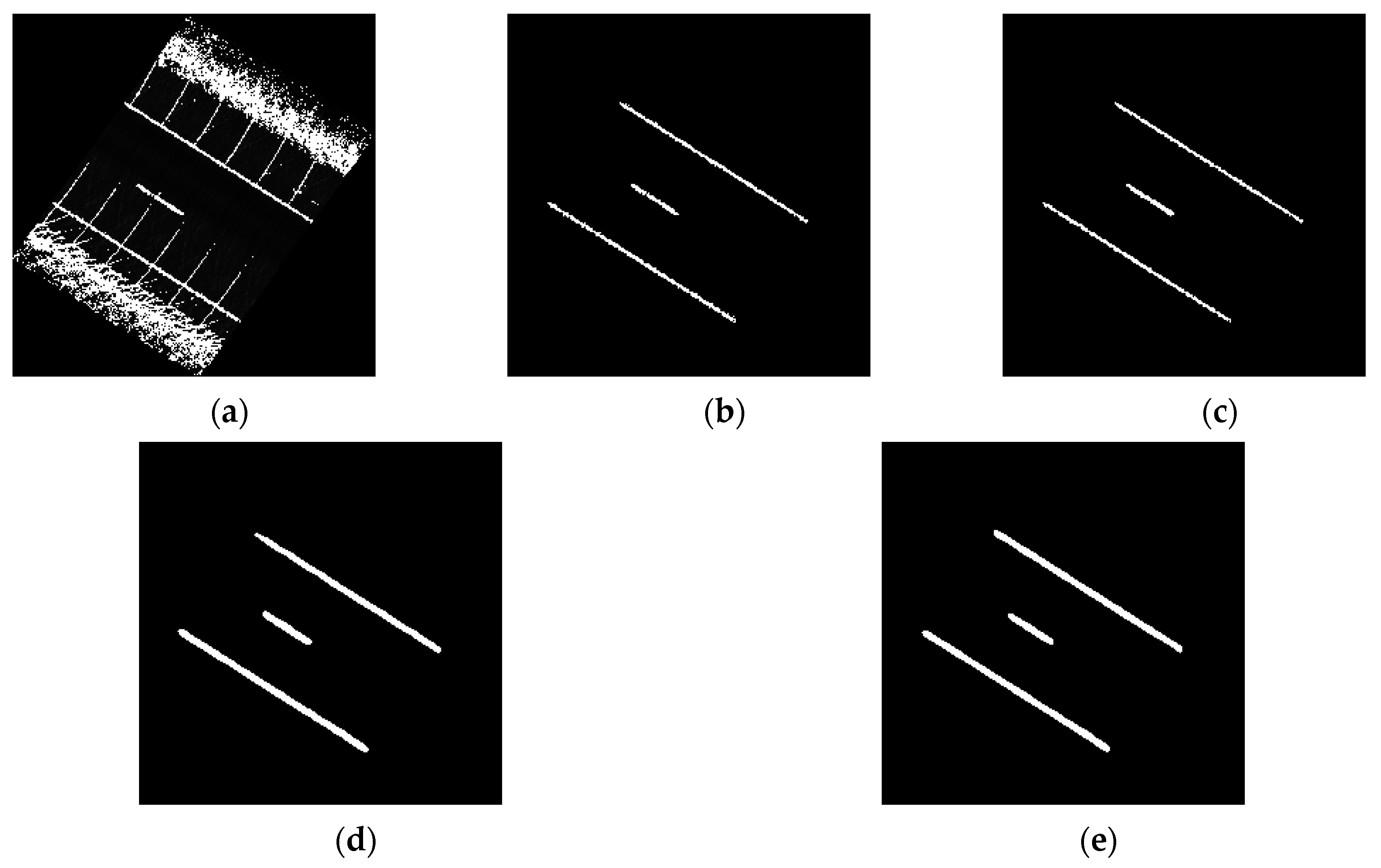
• In asphalt pavement area, the results from the different strategies are comparable except for the right lane markings where U-net model 1 has poor performance. The results of model 1 are unexpected, and it is hypothesized that this is a result of unintended adversarial noise [34] in intensity images generated for these areas.
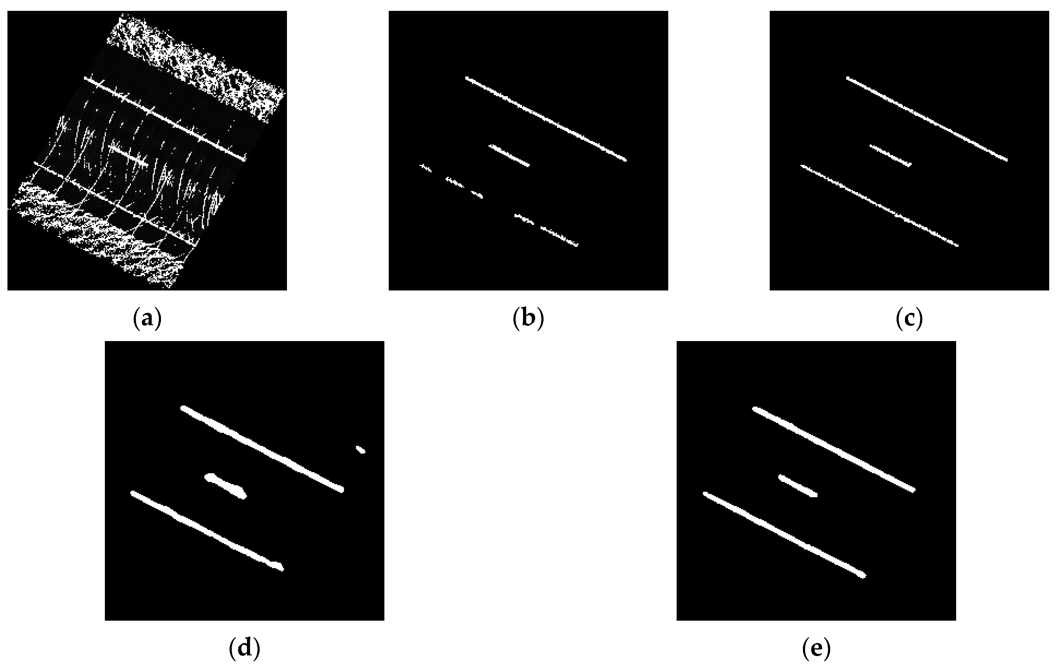
• In concrete pavement area (however), U-net model 2 can extract much longer length of the left lane markings compared to other strategies. For the center lane markings, the normalized intensity thresholding strategy results in the largest lane marking extraction followed by the deep learning approaches. The right lane markings have consistent results under all strategies since it is near the driving lane where the lane markings have high point density. Overall, we conclude that the normalized intensity thresholding and deep learning approaches can extract lane marking much better than the original intensity thresholding strategy in concrete pavement area.

5.2. Lane Width Estimation Results

In this section, we compare the lane width estimation results for all strategies across the three datasets. As mentioned previously, an estimate of the lane width is automatically derived every 20 cm using the approach proposed by Ravi et al. [18]. Depending on the starting position for lane width estimation, which depends on the extracted lane markings, the locations of lane width estimates might slightly differ from one strategy to another. Thus, for lane width comparison, a difference is calculated if the distance between two estimates is less than 20 cm. Consequently, the number of comparisons is slightly different for each strategy. Throughout the following comparisons, lane width values based on the normalized intensity thresholding serve as the reference for comparison because its lane markings were used to automatically generate the training labels for U-net model 2. While explaining the different results, this section refers to lane markings before noise removal as “hypothesized lane marking points,” and the ones after noise removal as “lane marking centerline points.” Finally, the section concludes with a quantitative comparison between manually evaluated and automatically derived lane width estimates from different strategies.

5.2.1. Datasets 1 and 2: Mainly Asphalt Pavement

For dataset 1,

Table 8. Lane width difference statistics for different lane marking extraction strategies in dataset 1.

Strategy	Original Intensity Thresholding		Normalized Intensity Thresholding		Deep Learning with Manual Labeling		Deep Learning with Automated Labeling
Lane	1	2	1	2	1	2	1	2
Length of Dataset (mile)	18.04
Estimated Length (mile)	17.74	15.22	17.81	15.11	17.79	15.90	17.68	15.70
# of Comparisons	142,689	121,115	-	-	142,312	121,615	141,424	121,256
Mean (cm)	0.2	−0.3	-	-	0.2	−0.4	0.3	−0.5
STD (cm)	1.1	1.1	-	-	1.3	1.3	1.2	1.3
RMSE (cm)	1.1	1.1	-	-	1.3	1.3	1.3	1.4
Max. (cm)	7.0	13.3	-	-	18.5	13.2	16.8	15.6
Min. (cm)	−7.0	−7.2	-	-	−19.8	−10.9	−11.7	−16.1

Note: compared with normalized intensity thresholding lane width estimates.

lists the number of comparisons, estimated length (total distance over which lane width estimates are obtained), and difference statistics for the four strategies. The lane width estimates in dataset 1 using various strategies are illustrated in Figure 28. These results indicate that lane width estimates from the intensity thresholding approaches are similar. Lane width estimates from the normalized intensity thresholding, on the other hand, differ from the ones obtained from the deep learning approaches. This difference is attributed to the fact that the deep learning approaches, with higher recall values, extract most of the actual lane markings including worn-out lane markings, which might be missed by thresholding strategies (i.e., more interpolation is conducted for the intensity thresholding strategies). Additionally, compared with the mean values of the differences in lane 1, the mean values in lane 2 are higher for all strategies because of the large scanning distance over lane 2 resulting in sparse point density and lower accuracy of the derived road surface point cloud. Due to the same reason, the total length of the highway, where lane width estimates are reported, is less in lane 2 for all strategies. However, the deep learning approaches can deliver lane width estimates over a longer length in lane 2 than intensity thresholding approaches. This is consistent with the previous discussion that the deep learning approaches can detect a complete edge lane marking with low point density, as shown in Figure 22.

To further evaluate the strategies, we also processed dataset 2, which is mainly asphalt pavement but has more concrete pavements than dataset 1. The lane width estimates in dataset 2 from the different lane marking extraction strategies are presented in Figure 29. The number of comparisons, estimated length, and difference statistics for dataset 2 are summarized in

Table 9. Lane width difference statistics for different lane marking extraction strategies in dataset 2.

Strategy	Original Intensity Thresholding		Normalized Intensity Thresholding		Deep Learning with Manual Labeling		Deep Learning with Automated Labeling
Lane	1	2	1	2	1	2	1	2
Length of Dataset (mile)	33.87
Estimated Length (mile)	23.31	21.52	24.37	22.33	30.18	26.79	29.12	25.66
# of Comparisons	176,316	162,047	-	-	194,015	177,399	188,888	175,347
Mean (cm)	0.0	0.1	-	-	−0.1	0.3	0.0	0.3
STD (cm)	1.8	2.1	-	-	2.2	2.4	2.3	3.0
RMSE (cm)	1.8	2.1	-	-	2.2	2.4	2.3	3.0
Max. (cm)	21.2	23.3	-	-	17.7	24.0	40.3	59.8
Min. (cm)	−23.0	−28.8	-	-	−19.4	−24.8	−18.3	−40.1

Note: compared with normalized intensity thresholding lane width estimates.

. The normalized intensity thresholding strategy produces lane width estimates over a larger distance when compared to the strategy using original intensity values in both lanes. Compared with the intensity thresholding approaches, as shown as the red box in Figure 29, more lane width values were estimated using the deep learning approaches, especially in poor lane marking areas. The hypothesized lane markings, lane marking centerline points, and interpolated points obtained from the different strategies in such area (red box in Figure 29) are illustrated in Figure 30. From this figure, we can observe that worn-out lane markings were removed by the minimum point threshold (Th_pt). However, they were kept in the deep learning approaches due to the minimum area threshold (Th_area), which was applied to 3D masks generated from its predictions. It is also observed that U-net model 1 results in almost 1-mile longer lane width estimation than U-net model 2 in both lanes. This longer estimation is owed to a higher recall rate of 98.9% in U-net model 1, as reported in Table 7. However, U-net model 1, with the low precision of 60.5%, needs higher computation time than model 2 for eliminating many false positives through the noise removal strategies. In this dataset, it took approximately 22 min for noise removal from the results from U-net model 1 and around 18 min for model 2.

5.2.2. Dataset 3: Mainly Concrete Pavement

For dataset 3, Figure 31 shows the lane width profile derived from the different lane marking extraction strategies, and

Table 10. Lane width difference statistics for different lane marking extraction strategies in dataset 3.

Strategy	Original Intensity Thresholding		Normalized Intensity Thresholding		Deep Learning with Manual Labeling		Deep Learning with Automated Labeling
Lane	1	2	1	2	1	2	1	2
Length of Dataset (mile)	15.29
Estimated Length (mile)	14.50	13.88	14.98	14.28	14.53	14.37	14.66	14.39
# of Comparisons	116,432	111,426	-	-	116,851	112,660	117,905	112,955
Mean (cm)	0.1	−0.1	-	-	0.1	−0.2	0.0	−0.1
STD (cm)	2.4	2.3	-	-	1.9	2.2	1.1	1.5
RMSE (cm)	2.4	2.3	-	-	1.9	2.2	1.1	1.5
Max. (cm)	53.7	25.4	-	-	40.4	15.8	58.9	14.2
Min. (cm)	−24.7	−32.4	-	-	−13.2	−34.3	−19.4	−32.9

Note: compared with normalized intensity thresholding lane width estimates.

summarizes the number of comparisons, estimated length, and difference statistics among the four strategies. As shown in Figure 31, it is apparent that lane width estimates obtained from the original intensity thresholding strategy and deep learning approaches differ significantly from the normalized intensity thresholding strategy in some areas. The RGB imagery for two such areas are shown in Figure 32a,b, also indicated as red boxes I and II in Figure 31. Referring to the red box I in Figure 31, hypothesized lane markings, lane marking centerline points, and interpolated centerline points for all lane marking extraction strategies are displayed in Figure 32c. This figure shows that five dash lane markings were not extracted using the intensity thresholding strategy due to higher noise in concrete pavement. Figure 32d, which refers to the red box II in Figure 31, compares hypothesized lane markings, lane marking centerline points, and interpolated centerline points obtained from the different strategies. Three dash lane markings were not detected in the deep learning strategy using U-net model 2. This misdetection is caused by the training data bias of U-net model 2, as shown in Figure 23.

In summary, the performance of the original intensity thresholding strategy gradually declines with an increase in the area of concrete pavement, but the other three strategies can extract more lane markings in such area as validated by a longer distance where lane width estimates are reported across all datasets. The longer lengths for lane width estimation in dataset 2 for both lanes confirm the claim that the deep learning approaches perform better in areas of worn-out edge lane markings when compared to intensity thresholding strategies. The standard deviations of the difference statistics for all datasets, which range from 1.1 to 3.0 cm, indicating that the lane width estimates from the different strategies are compatible within a 1 to 3 cm range.

5.2.3. Comparison With Manual Lane Width Measurements

In order to demonstrate the robustness of the lane marking extraction and lane width estimation strategies, the automatically derived lane width estimates are compared to manually evaluated ones for all datasets. Figure 33 shows a road surface point cloud and manually established points for lane width estimation. For manual lane width estimation, two points are defined on a dash line, and another point is defined on the corresponding edge lane marking. The two points on the dash lane marking are used to derive a line through them. The third point on the edge lane marking is projected onto that line. Finally, a 3D distance between the point along the edge lane marking and its projection on the dash lane marking is used as the manually evaluated lane width. One should note that we used the dash lane marking to define the lane width direction since it is usually straight (in contrast to edge lane markings that could be curved).

A lane width difference is calculated if the distance between the manual and automated estimates is less than 20 cm apart as per the Th_dist threshold. Although the same manually evaluated lane width estimates are used to examine the lane width estimates in each dataset, the number of comparisons is different for each strategy due to the expected variation in the locations of automatically derived lane width estimates. The quantitative metrics, including the mean, standard deviation, root-mean-square error (RMSE), and maximum difference between the manually and automatically evaluated lane width estimates are summarized in

Table 11. Lane width difference statistics between various strategies and manual measurements.

Dataset	Strategy	Original Intensity Thresholding		Normalized Intensity Thresholding		Deep Learning with Manual Labeling		Deep Learning with Automated Labeling
	Lane	1	2	1	2	1	2	1	2
1	Length of Dataset (mile)	18.04
	Estimated Length (mile)	17.74	15.22	17.81	15.11	17.79	15.90	17.68	15.70
	# of Comparisons	150	148	149	146	147	153	149	152
	Mean (cm)	0.9	1.2	0.6	1.3	1.0	1.2	0.9	1.1
	STD (cm)	2.3	2.4	2.5	2.4	2.3	2.5	2.4	2.4
	RMSE (cm)	2.5	2.7	2.6	2.7	2.5	2.7	2.6	2.6
	Max. (cm)	6.9	6.2	6.6	6.9	6.6	6.6	6.9	7.0
	Min. (cm)	−4.6	−5.2	−5.6	−5.9	−4.7	−6.8	−3.9	−5.4
2	Length of Dataset (mile)	33.87
	Estimated Length (mile)	23.31	21.52	24.37	22.33	30.18	26.79	29.12	25.66
	# of Comparisons	176	204	190	204	218	222	215	219
	Mean (cm)	−0.4	−0.4	−0.2	−0.3	−0.4	−0.6	−0.3	−0.4
	STD (cm)	2.4	2.6	2.5	2.7	2.4	2.6	2.5	2.8
	RMSE (cm)	2.4	2.6	2.5	2.7	2.4	2.6	2.5	2.8
	Max. (cm)	6.7	6.5	6.5	6.5	4.9	6.8	6.9	6.9
	Min. (cm)	−6.6	−6.7	−6.3	−6.0	−6.8	−6.8	−6.5	−6.5
3	Length of Dataset (mile)	15.29
	Estimated Length (mile)	14.50	13.88	14.98	14.28	14.53	14.37	14.66	14.39
	# of Comparisons	196	181	204	192	200	192	203	193
	Mean (cm)	0.3	0.4	0.3	0.4	0.3	0.3	0.3	0.4
	STD (cm)	1.2	1.5	1.2	1.5	1.4	1.5	1.3	1.5
	RMSE (cm)	1.2	1.6	1.3	1.5	1.4	1.6	1.4	1.5
	Max. (cm)	3.5	5.0	3.7	4.8	3.9	6.6	6.5	4.8
	Min. (cm)	−3.1	−4.3	−4.8	−3.4	−6.1	−4.5	−5.4	−3.5

. Overall, there is no difference greater than 7 cm for all datasets, and the RMSE values of the differences range from 1.2 to 2.8 cm, indicating good agreement among the manually and automatically-evaluated estimates. Moreover, the differences are coherent with the 2–4 cm expected accuracy range of the point cloud for the used system. The slightly larger mean differences in lane 2 reflect the slightly poor accuracy for points with longer scanning distance.

5.3. Lane Marking Gap Results

As mentioned previously, all the datasets include center, left, and right lane markings, as shown in Figure 27a. For each dataset, derived lane markings from the normalized intensity thresholding strategy are used to report right and left lane marking gaps (i.e., along edge lane markings) while U-net model 2 results are utilized to report the same along center (i.e., along dash lane markings). One should note that in all the datasets, the left lane markings are yellow edge lines, while the center and right lane markings are white dash and edge lines, respectively. For the different datasets, the driving lane, which is bounded by the center and right lane markings, was maintained during the data collection. The long lane marking gap regions along the road surface for the three datasets are reported in Figure 34. The figure also shows an example of a location with a long gap (more than Th_miss) for each of the datasets. It can be seen that the dash lane markings in Figure 34b,c are obviously worn-out or missing (identified through U-net model 2) in the RGB imagery, while the yellow markings in Figure 34a are slightly worn (identified through normalized thresholding strategy) in the image. The total length and average (total length of the gaps divided by the length of the dataset) of long lane marking gaps in datasets 1, 2, and 3 are summarized in

Table 12. Statistics of long lane marking gaps for datasets 1, 2, and 3.

Dataset	Length of Dataset	Lane Marking	# of Long Gaps	Total Length of Long Gaps (ft)	Average Gap (ft/mile)
1	18.04 mile	Left	29	7431.8 (2265.2 m)	412.0
		Center	1	151.0 (46.0 m)	8.4
		Right	0	0.0 (0.0 m)	0.0
2	33.87 mile	Left	41	15,392.7 (4691.7 m)	454.5
		Center	14	3608.2 (1099.8 m)	106.5
		Right	0	0.0 (0.0 m)	0.0
3	15.29 mile	Left	16	3107.0 (947.0 m)	203.2
		Center	6	1136.7 (346.5 m)	74.3
		Right	0	0.0 (0.0 m)	0.0

. On the other hand, short lane marking gap regions along center, left, and right lane markings for the three datasets are reported in Figure 35, which also shows an example of a location with a short gap (less than Th_miss). The RGB imagery in Figure 35 shows the worn-out lane markings at locations i, ii, and iii for datasets 1, 2, and 3, respectively. Overall, this reporting algorithm quickly identifies a large number of regions that require further visual inspection, which can reduce cost and time for on-site inspections.

6. Conclusions and Recommendations for Future Research

Lane marking extraction through intensity thresholding of LiDAR-based MMS point clouds has traditionally suffered from the problem of large false positives. Hence, prior knowledge is required for noise removal. In contrast, learning-based approaches can detect lane markings from an intensity image without a specific prerequisite, but they are limited by the tedious procedure of manual labeling for training data generation. In this paper, in order to address these challenges, normalized intensity thresholding and deep learning strategies with automatically generated labels are proposed for extracting lane markings from LiDAR-based MMS point clouds. To test the performance of the proposed strategies, an original intensity thresholding strategy and a deep learning strategy using manually established labels are also implemented. In addition, the performance evaluation of all strategies is also carried out in asphalt and concrete pavement areas. For the original and normalized intensity thresholding strategies, lane markings were directly extracted from the road surface point cloud. For the deep learning approaches, lane markings were detected from generated intensity images using U-net models trained on manually established (model 1) and automatically-generated labels (model 2). Additionally, the lane markings extracted through the normalized intensity thresholding strategy and U-net model 2 were used to report lane marking gap regions along edge lines and dash lines, respectively. Lastly, the lane marking derived from all strategies are utilized for lane width estimation.

In this research, three datasets, with a total length of about 67 miles, were surveyed on two-lane highways that covered both concrete and asphalt pavement areas. Compared with the lane markings from thresholding of the original intensity, hypothesized lane markings derived from the normalized intensity thresholding strategy have less false positives. On the other hand, U-net model 2 performs better than model 1, as indicated by a higher F1-score. The precision, recall, and F1-score obtained for U-net model 1 are 60.5%, 98.9%, and 75.1%, respectively. Moreover, the derived precision, recall, and F1-score for U-net model 2 are 84%, 87.9%, and 85.9%, respectively. Further, the same metrics for the normalized intensity thresholding strategy were obtained as 83.9%, 74.4%, and 78.9%, respectively, indicating a performance better than U-net model 1 but not model 2. The original intensity thresholding strategy has an inferior overall performance than the above strategies with an F1-score of 72.3%. In concrete pavement area, high-intensity outliers are successfully eliminated by the normalized intensity thresholding and both deep learning strategies, unlike the thresholding of original intensity values. In addition, the lane width estimation results demonstrate that the deep learning approaches could extract more lane markings than other strategies in poor edge lane marking area and non-driving lane. Since this research is based on an MMS equipped with accurately calibrated imaging and ranging systems, reported lane marking gaps can be visually inspected in the RGB imagery to evaluate the cause of such gaps (e.g., missing and/or worn-out lane markings).

Future research will focus on developing an intensity normalization algorithm for an MMS equipped with single-beam LiDAR scanners. According to the assumption that the intensity values across laser beams should be similar for the same surface, utilization of an MMS equipped with two or more single-beam LiDAR scanners should also achieve the same intensity normalization effect. Another focus will be to increase the number of training samples for the U-net model trained on automatically generated labels by including samples from other single-beam LiDAR datasets. This will enhance the generalization capability of the U-net model across different types of sensors as well as improve the detection results on problematic cases such as worn-out dash lane markings with low point density. Additionally, the RGB information from imagery will be combined with point cloud data to improve the accuracy of lane marking extraction (especially those that are worn-out).

References

1. Hernández, D.C.; Seo, D.; Jo, K.-H. Robust lane marking detection based on multi-feature fusion. In Proceedings of the 2016 9th International Conference on Human System Interactions (HSI), Portsmouth, UK, 6–8 July 2016; pp. 423–428. [Google Scholar]
2. Jung, S.; Youn, J.; Sull, S. Efficient lane detection based on spatiotemporal images. IEEE Trans. Intell. Transp. Syst. 2015, 17, 289–295. [Google Scholar] [CrossRef]
3. Azimi, S.M.; Fischer, P.; Körner, M.; Reinartz, P. Aerial LaneNet: Lane-marking semantic segmentation in aerial imagery using wavelet-enhanced cost-sensitive symmetric fully convolutional neural networks. IEEE Trans. Geosci. Remote Sens. 2018, 57, 2920–2938. [Google Scholar] [CrossRef] [Green Version]
4. LeCun, Y.; Haffner, P.; Bottou, L.; Bengio, Y. Object recognition with gradient-based learning. In Shape, Contour and Grouping in Computer Vision; Springer: Berlin/Heidelberg, Germany, 1999; pp. 319–345. [Google Scholar]
5. Guan, H.; Li, J.; Yu, Y.; Wang, C.; Chapman, M.; Yang, B. Using mobile laser scanning data for automated extraction of road markings. ISPRS J. Photogramm. Remote Sens. 2014, 87, 93–107. [Google Scholar] [CrossRef]
6. Kumar, P.; McElhinney, C.P.; Lewis, P.; McCarthy, T. Automated road markings extraction from mobile laser scanning data. Int. J. Appl. Earth Obs. Geoinf. 2014, 32, 125–137. [Google Scholar] [CrossRef] [Green Version]
7. Soilán, M.; Riveiro, B.; Martínez-Sánchez, J.; Arias, P. Segmentation and classification of road markings using MLS data. ISPRS J. Photogramm. Remote Sens. 2017, 123, 94–103. [Google Scholar] [CrossRef]
8. Cheng, M.; Zhang, H.; Wang, C.; Li, J. Extraction and classification of road markings using mobile laser scanning point clouds. IEEE J. Sel. Top. Appl. Earth Obs. Remote Sens. 2016, 10, 1182–1196. [Google Scholar] [CrossRef]
9. Ghallabi, F.; Nashashibi, F.; El-Haj-Shhade, G.; Mittet, M.-A. Lidar-based lane marking detection for vehicle positioning in an hd map. In Proceedings of the 2018 21st International Conference on Intelligent Transportation Systems (ITSC), Maui, HI, USA, 4–7 November 2018; pp. 2209–2214. [Google Scholar]
10. Jung, J.; Che, E.; Olsen, M.J.; Parrish, C. Efficient and robust lane marking extraction from mobile lidar point clouds. ISPRS J. Photogramm. Remote Sens. 2019, 147, 1–18. [Google Scholar] [CrossRef]
11. Yu, Y.; Li, J.; Guan, H.; Jia, F.; Wang, C. Learning hierarchical features for automated extraction of road markings from 3-D mobile LiDAR point clouds. IEEE J. Sel. Top. Appl. Earth Obs. Remote Sens. 2015, 8, 709–726. [Google Scholar] [CrossRef]
12. Yan, L.; Liu, H.; Tan, J.; Li, Z.; Xie, H.; Chen, C. Scan line based road marking extraction from mobile LiDAR point clouds. Sensors 2016, 16, 903. [Google Scholar] [CrossRef] [PubMed]
13. Jeong, J.; Kim, A. Lidar intensity calibration for road marking extraction. In Proceedings of the 2018 15th International Conference on Ubiquitous Robots (UR), Honolulu, HI, USA, 26–30 June 2018; pp. 455–460. [Google Scholar]
14. He, B.; Ai, R.; Yan, Y.; Lang, X. Lane marking detection based on convolution neural network from point clouds. In Proceedings of the 2016 IEEE 19th International Conference on Intelligent Transportation Systems (ITSC), Rio de Janeiro, Brazil, 1–4 November 2016; pp. 2475–2480. [Google Scholar]
15. Wen, C.; Sun, X.; Li, J.; Wang, C.; Guo, Y.; Habib, A. A deep learning framework for road marking extraction, classification and completion from mobile laser scanning point clouds. ISPRS J. Photogramm. Remote Sens. 2019, 147, 178–192. [Google Scholar] [CrossRef]
16. Hartigan, J.A.; Hartigan, P.M. The dip test of unimodality. Ann. Stat. 1985, 13, 70–84. [Google Scholar] [CrossRef]
17. Ronneberger, O.; Fischer, P.; Brox, T. U-net: Convolutional networks for biomedical image segmentation. In Proceedings of the International Conference on Medical Image Computing and Computer-Assisted Intervention; Springer: Cham, Switzerland, 2015; pp. 234–241. [Google Scholar]
18. Ravi, R.; Cheng, Y.-T.; Lin, Y.-C.; Lin, Y.-J.; Hasheminasab, S.M.; Zhou, T.; Flatt, J.E.; Habib, A. Lane Width Estimation in Work Zones Using LiDAR-Based Mobile Mapping Systems. IEEE Trans. Intell. Transp. Syst. 2019, 1–24. [Google Scholar] [CrossRef]
19. Velodyne. HDL32E Data Sheet. Available online: https://velodynelidar.com/products/hdl-32e/ (accessed on 10 February 2020).
20. Velodyne. Puck Hi-Res Data Sheet. Available online: https://velodynelidar.com/products/puck-hi-res/ (accessed on 10 February 2020).
21. Applanix. POSLV Specifications. Available online: https://www.applanix.com/pdf/specs/POSLV_Specifications_dec_2015.pdf (accessed on 10 February 2020).
22. Habib, A.; Lay, J.; Wong, C. Specifications for the quality assurance and quality control of lidar systems. In Proceedings of the Innovations in 3D Geo Information Systems; Springer: Berlin/Heidelberg, Germany, 2006; pp. 67–83. [Google Scholar]
23. Ravi, R.; Lin, Y.-J.; Elbahnasawy, M.; Shamseldin, T.; Habib, A. Bias impact analysis and calibration of terrestrial mobile lidar system with several spinning multibeam laser scanners. IEEE Trans. Geosci. Remote Sens. 2018, 56, 5261–5275. [Google Scholar] [CrossRef]
24. Ravi, R.; Lin, Y.-J.; Elbahnasawy, M.; Shamseldin, T.; Habib, A. Simultaneous system calibration of a multi-lidar multicamera mobile mapping platform. IEEE J. Sel. Top. Appl. Earth Obs. Remote Sens. 2018, 11, 1694–1714. [Google Scholar] [CrossRef]
25. Lari, Z.; Habib, A. New approaches for estimating the local point density and its impact on LiDAR data segmentation. Photogramm. Eng. Remote Sens. 2013, 79, 195–207. [Google Scholar] [CrossRef]
26. Levinson, J.; Thrun, S. Robust vehicle localization in urban environments using probabilistic maps. In Proceedings of the 2010 IEEE International Conference on Robotics and Automation, Anchorage, AK, USA, 3–7 May 2010; pp. 4372–4378. [Google Scholar]
27. Levinson, J.; Thrun, S. Unsupervised calibration for multi-beam lasers. In Proceedings of the Experimental Robotics; Springer: Berlin/Heidelberg, Germany, 2014; pp. 179–193. [Google Scholar]
28. Ioffe, S.; Szegedy, C. Batch normalization: Accelerating deep network training by reducing internal covariate shift. arXiv preprint 2015, arXiv:1502.03167. [Google Scholar]
29. Dice, L.R. Measures of the amount of ecologic association between species. Ecology 1945, 26, 297–302. [Google Scholar] [CrossRef]
30. FHWA. Manual on Uniform Traffic Control Devices 2009; USD o. Transportation: Washington, DC, USA, 2009.
31. Fischler, M.A.; Bolles, R.C. Random sample consensus: A paradigm for model fitting with applications to image analysis and automated cartography. Commun. ACM 1981, 24, 381–395. [Google Scholar] [CrossRef]
32. AASHTO. A Policy on Geometric Design of Highways and Streets, 7th ed.; American Association of State Highway and Transportation Officials: Washington, DC, USA, 2001. [Google Scholar]
33. USGS. Materials in Use in U.S. Interstate Highway. Available online: https://pubs.usgs.gov/fs/2006/3127/2006-3127.pdf (accessed on 10 February 2020).
34. Goodfellow, I.J.; Shlens, J.; Szegedy, C. Explaining and harnessing adversarial examples. arXiv preprint 2014, arXiv:1412.6572. [Google Scholar]
Figure 1. The mobile mapping system Purdue Wheel-based Mobile Mapping System-High Accuracy (PWMMS-HA) used in this research.
Remotesensing 12 01379 g001
Figure 2. Projection of a location (red dot) in a Light Detection and Ranging (LiDAR) point cloud onto the corresponding RGB imagery (empty magenta circle) using the estimated LiDAR/camera/GNSS/IMU system calibration parameters.
Remotesensing 12 01379 g002
Figure 3. Location, trajectory, concrete pavement distribution, and regions of interest (ROIs) for generating intensity normalization maps of (a) dataset 1, (b) dataset 2, and (c) dataset 3.
Remotesensing 12 01379 g003
Figure 4. Flowchart of the proposed framework for lane marking extraction and lane width estimation.
Remotesensing 12 01379 g004
Figure 5. Illustrations of (a) hypothesized lane markings extracted by simple thresholding of the original intensity values and (b) corresponding RGB imagery in asphalt pavement area.
Remotesensing 12 01379 g005
Figure 6. Illustrations of (a) hypothesized lane markings extracted by simple thresholding of the original intensity values and (b) the corresponding RGB imagery in concrete pavement area.
Remotesensing 12 01379 g006
Figure 7. Flowchart of the normalized intensity thresholding strategy for a multi-beam LiDAR-based MMS.
Remotesensing 12 01379 g007
Figure 8. Flowchart of the proposed deep learning lane marking extraction and U-net model training framework.
Remotesensing 12 01379 g008
Figure 9. Schematic diagram of a road surface point cloud block used for intensity image generation.
Remotesensing 12 01379 g009
Figure 10. Illustrations of (a) original road surface point cloud block and (b) corresponding intensity image.
Remotesensing 12 01379 g010
Figure 11. Illustrations of derived lane markings from (a) normalized intensity thresholding, (b) normalized intensity thresholding after noise removal, (c) bounding boxes (in red) encompassing lane markings, and (d) labeled image.
Remotesensing 12 01379 g011
Figure 12. Implemented U-net architecture for the deep learning-based strategy for lane marking extraction (adapted from Ronneberger et al. [17]).
Remotesensing 12 01379 g012
Figure 13. U-net prediction refinement: (a) mask regions formed by 5-cm cells, (b) two-dimensional (2D) masks overlaid on points whose intensity is in the 5th percentile intensity of the original point cloud, and (c) predicted lane markings.
Remotesensing 12 01379 g013
Figure 14. Lane marking centerline derivation framework (adapted from Ravi et al. [18]).
Remotesensing 12 01379 g014
Figure 15. Illustrations of (a) hypothesized lane marking segments, (b) segments after RANSAC-based noise removal, and (c) segments after trajectory-based noise removal.
Remotesensing 12 01379 g015
Figure 16. Illustration of (a) lane marking centerline grouping and (b) interpolation for filling the gap which is larger than Thdist and less than Thmiss (adapted from Ravi et al. [18]).
Remotesensing 12 01379 g016
Figure 17. Illustration of gaps along (a) dash and (b) edge lines reported as short lane marking gap regions.
Remotesensing 12 01379 g017
Figure 18. Intensity normalization maps associated with an HDL 32E LiDAR unit for (a) ROI 1, (b) ROI 2, and (c) ROI 3.
Remotesensing 12 01379 g018
Figure 19. Intensity normalization maps associated with an HDL 32E LiDAR unit for (a) ROI 1, (b) ROI 2, and (c) ROI 3.
Remotesensing 12 01379 g019aRemotesensing 12 01379 g019b
Figure 20. Training and validation loss curves for (a) U-net model 1 and (b) U-net model 2.
Remotesensing 12 01379 g020
Figure 21. RGB imagery of (a) location i and (b) location ii and illustrations of (c) original intensity images, and images with predicted lane markings from (d) U-net model 1 and (e) U-net model 2 in dataset 2.
Remotesensing 12 01379 g021
Figure 22. Yellow edge lane marking area in dataset 2: (a) RGB imagery of location i, (b) original intensity image, predicted lane marking images of (c) original intensity thresholding, (d) normalized intensity thresholding, (e) U-net model 1, and (f) U-net model 2.
Remotesensing 12 01379 g022aRemotesensing 12 01379 g022b
Figure 23. Worn-out dash lane marking area in dataset 3: (a) RGB imagery of location i, (b) original intensity image, predicted lane marking images of (c) original intensity thresholding, (d) normalized intensity thresholding, (e) U-net model 1, and (f) U-net model 2.
Remotesensing 12 01379 g023
Figure 24. Illustrations of intensity images in (a) asphalt pavement area and (b) concrete pavement area, and corresponding RGB imagery for (c) location i and (d) location ii in dataset 3.
Remotesensing 12 01379 g024
Figure 25. Asphalt pavement area (for location i in Figure 24): (a) original intensity image and predicted lane marking images from (b) original intensity thresholding, (c) normalized intensity thresholding, (d) U-net model 1, and (e) U-net model 2.
Remotesensing 12 01379 g025
Figure 26. Concrete pavement area (for location ii in Figure 24): (a) original intensity image and predicted lane marking images from (b) original intensity thresholding, (c) normalized intensity thresholding, (d) U-net model 1, and (e) U-net model 2.
Remotesensing 12 01379 g026
Figure 27. Illustrations of (a) lane marking schematic diagram and length of lane markings extracted from different strategies in (b) asphalt pavement areas and (c) concrete pavement areas for dataset 3.
Remotesensing 12 01379 g027
Figure 28. Estimated lane width values in (a) lane 1 and (b) lane 2 for dataset 1.
Remotesensing 12 01379 g028
Figure 29. Estimated lane width values in (a) lane 1 and (b) lane 2 for dataset 2.
Remotesensing 12 01379 g029
Figure 30. (a) RGB imagery and illustrations of (b) hypothesized lane markings (left), and lane marking centerline and interpolated points overlaid on the same hypothesized lane markings (right) in a poor lane marking area (red box in Figure 29) for dataset 2.
Remotesensing 12 01379 g030
Figure 31. Estimated lane width values in (a) lane 1 and (b) lane 2 for dataset 3.
Remotesensing 12 01379 g031
Figure 32. RGB imagery in (a) location i and (b) location ii, and illustrations of hypothesized lane markings (left), and lane marking centerline and interpolated points overlaid on the same hypothesized lane markings (right) in concrete pavement areas for the red boxes (c) I and (d) II in Figure 31 for dataset 3.
Remotesensing 12 01379 g032aRemotesensing 12 01379 g032b
Figure 33. Road surface point cloud and points used for manual evaluation of lane width estimates.
Remotesensing 12 01379 g033
Figure 34. Illustrations of long lane marking gap regions versus mile marker (top) together with an example location defined by start and end points overlaid on hypothesized lane markings (bottom-left) and corresponding RGB imagery (bottom-right) for (a) dataset 1, (b) dataset 2, and (c) dataset 3.
Remotesensing 12 01379 g034
Figure 35. Illustrations of short lane marking gap regions versus mile marker (top) together with an example location defined by start and end points overlaid on hypothesized lane markings (bottom-left), and corresponding RGB imagery (bottom-right) for (a) dataset 1, (b) dataset 2, and (c) dataset 3.
Remotesensing 12 01379 g035