Habitat Suitability Estimation Using a Two-Stage Ensemble Approach

Abstract

Biodiversity conservation is important for the protection of ecosystems. One key task for sustainable biodiversity conservation is to effectively preserve species’ habitats. However, for various reasons, many of these habitats have been reduced or destroyed in recent decades. To deal with this problem, it is necessary to effectively identify potential habitats based on habitat suitability analysis and preserve them. Various techniques for habitat suitability estimation have been proposed to date, but they have had limited success due to limitations in the data and models used. In this paper, we propose a novel scheme for assessing habitat suitability based on a two-stage ensemble approach. In the first stage, we construct a deep neural network (DNN) model to predict habitat suitability based on observations and environmental data. In the second stage, we develop an ensemble model using various habitat suitability estimation methods based on observations, environmental data, and the results of the DNN from the first stage. For reliable estimation of habitat suitability, we utilize various crowdsourced databases. Using observational and environmental data for four amphibian species and seven bird species in South Korea, we demonstrate that our scheme provides a more accurate estimation of habitat suitability compared to previous other approaches. For instance, our scheme achieves a true skill statistic (TSS) score of 0.886, which is higher than other approaches (TSS = 0.725 ± 0.010).

1. Introduction

For decades, the importance of biodiversity conservation has been emphasized globally because high biodiversity offers a variety of natural services that support sustainable human living [1]. Despite this importance, ecosystem services have rapidly declined for a variety of reasons, such as indiscriminate resource development, rapid urban expansion, and global climate change. The loss of biodiversity can have adverse consequences on the ecosystem because of the complex interactions that exist among species [2,3]. To maintain biodiversity levels, ecologists have devised and applied various methods to protect habitats by analyzing the characteristics of target species and their habitats [4,5].

Habitat suitability models, also known as species distribution models (SDMs), environmental niche models (ENMs), and predictive habitat distribution models, have been used to predict the habitat of target species based on various environmental factors, such as temperature, precipitation, seasonality, and terrain [2,3,6]. Habitat suitability models can be used to assess not only the relationship among various environmental factors, such as global climatic conditions, landscape information, and species habitats, but also landscape management and the conservation of endangered species [6,7,8,9]. With the development of remote sensing technology, the performance of habitat suitability models has improved significantly. Until a few decades ago, the prediction of habitat suitability for particular species over a wide range of areas with reasonable accuracy was very challenging. This is because remote sensing technology at that time had several limitations, including high costs, poor spatial resolution, complicated digital maps at scales larger than remote sensing images, and human error during interpretation analysis. Recently, state-of-the-art remote sensing technologies have overcome previous data-processing issues, making it possible to obtain reliable temporal and spatial data for factors such as land cover and the climate and to subsequently construct inference models for habitat suitability that can cover very small to large areas.

Based on remote sensing data, several ecological researchers have attempted to construct effective habitat suitability models using a profile, statistical, and machine learning methods (

Table 1. Overview of habitat suitability modeling techniques.

Models	Descriptions	References	Category
SRE	Profiling technique that uses the environmental conditions of locations of occurrence data to profile the environments where a species can be found.	Araújo et al. [7], Heikkinen et al. [8], Thuiller et al. [9]	Profile
FDA	Classification technique based on a mixture of linear regression models.	Hastie et al. [14]	Statistical regression
GLM	Parametric regression technique based on a random component, a systematic component, and a link function describing a relation between the former the random and systematic component.	Elith et al. [10], Zuur et al. [12]	Statistical regression
MARS	Non-parametric regression technique that builds multiple linear regression models across the range of predictor values.	Elith et al. [10], Leathwick et al. [11], Friedman et al. [13],	Statistical regression
GBM	Machine learning technique based on the combinations of decision tree algorithms and boosting methods.	Thomaes et al. [20], De’Ath et al. [21]	Machine learning
CTA	Machine learning technique that is a supervised non-parametric statistical classification approach based on binary recursive partitioning techniques	Breiman et al. [22], De’ath G et al. [23]	Machine learning
SNN	Machine learning technique based on non-linear mapping structures inspired on the biological system of the brain.	D’heygere et al. [24], Fukuda et al. [25]	Machine learning
RF	Machine learning technique using bootstrap aggregation to create a set of decision trees.	Phillips et al. [17], Breiman L et al. [26], Cutler DR et al. [27]	Machine learning
MAXENT	Machine learning technique using the principle of maximum entropy to make a prediction from incomplete knowledge.	Phillips et al. [15], Reiss et al. [16]	Machine learning

). The surface range envelope (SRE) model, a profile approach, has been used to estimate habitat suitability [7,8,9]. Araújo et al. [7] introduced a series of surface envelop models based on the associations between climatic variables and the distributions of species to determine suitable conditions for the maintenance of a viable population. Heikkinen et al. [8] presented several critical methodological issues that may lead to uncertainty in predictions based on bioclimatic modeling. They concluded that bioclimatic envelop models have several advantages, one of which is that the modeling results are simple and easy to understand.

Statistical methods, such as flexible discriminant analysis (FDA), the multivariate adaptive regression spline (MARS), and the generalized linear model (GLM), investigate multiple linear relationships between species distributions and environmental layers. Statistical methods all have advantages and disadvantages, so various statistical methods are often employed together to improve habitat suitability estimation [10,11,12,13,14]. To determine the potential habitat and distribution of species, Elith et al. [10] presented a practical guide that included how to efficiently use statistical methods. They compared 16 modeling methods, including the MARS and GLM, using 226 species from six regions of the world. They found that the GLM, and BIOCLIM outperformed the other profile and statistical modeling methods. Leathwick et al. [11] utilized two statistical modeling methods, the generalized additive model (GAM) and MARS, to analyze the relationships between the distributions of 15 freshwater fish species and the corresponding environment. They reported that the MARS model performed strongly with low-prevalence species and that it could be used to analyze a large dataset.

Recently, habitat suitability modeling has been conducted using machine-learning methods, such as the generalized boosting model (GBM), maximum entropy (MAXENT), and random forest (RF). These machine-learning methods have been reported to produce more accurate predictions than profile and statistical methods [15,16,17,18,19,20,21,22,23,24,25,26,27]. For instance, Phillips et al. [15] utilized various machine-learning methods for the habitat modeling of ocean sunfish species. They used observations of ocean sunfishes and a number of environmental variables to conduct species distribution modeling using MARS, the SRE model, classification tree analysis (CTA), FDA, RF, and GLM. Reiss et al. [16] predicted the distribution of benthic species in the North Sea. They compared nine different methods: the support vector machine (SVM), GLM, GAM, GBM, MAXENT, FDA, BIOCLIM, and MARS. In their experiments, the machine-learning methods MAXENT, GBM, and RF produced a better predictive performance than the profile and statistical methods. Guisan et al. [17] employed various machine learning-based prediction methods to determine a suitable model for species habitats using remote sensing data. They examined multiple steps in predictive modeling by considering the conceptual model and its statistical formulation and calibration. Phillips et al. [18] employed maximum entropy-based modeling to predict the habitat of the Bradypus variegatus. They used two remote-sensed datasets, climate, and elevation that were derived from the Intergovernmental Panel on Climate Change (IPCC) and the United States Geological Survey (USGS), respectively. They evaluated the effectiveness of the model by comparing it to a rule-set-based genetic algorithm. Heikkinen et al. [19] conducted species habitat modeling for endangered butterfly species and predicted the distribution of Apollo butterflies using various machine-learning methods such as GLM, GAM, CTA, a shallow neural network (SNN), MARS, and boosted regression tree (BRT). They concluded that statistical analysis and machine-learning methods were useful for conservation planning and protecting endangered species.

More recently, habitat modeling based on deep neural networks (DNNs) has been investigated in ecological research [28,29,30,31]. In general, DNNs provide more accurate predictions in terms of identifying potential habitats for target species than conventional models such as GLM, GAM, MARS, and BRT. This is because DNNs can automatically extract features and learn complex non-linearities from extracted features [32]. For instance, Rademaker et al. [28] determined the niches of wild and domesticated ungulate species using modeling schemes based on a DNN. They focused on the applicability of the DNN and employed it in habitat estimation modeling. In their experiment, they showed that DNN could effectively identify potential habitats using sufficient observational data. Botella et al. [29] proposed a deep-learning approach for SDM. They applied a convolution neural network (CNN) and DNN to overcome the shortcomings of the traditional SDM. To evaluate its performance, they used part of the GBIF dataset and 46 environmental layers, including climate, digital elevation, and land cover. They subsequently found that both models performed better than traditional models such as the GAM and MAXENT.

However, despite the versatility of DNNs [30,31,32,33,34,35], a DNN-based habitat model trained on a small observational dataset for a species has been shown to produce inferior estimations to traditional machine-learning models, such as MAXENT and RF. Thus, constructing an accurate habitat suitability model is challenging because obtaining observational data is difficult [28]. Collecting sufficient observational data is particularly crucial when constructing habitat suitability models for endangered species. To overcome these problems, in this paper, we propose a novel two-stage based ensemble model called TSEM for the development of an effective habitat suitability model using an ensemble of various habitat suitability estimation techniques and DNN. Our TSEM was trained and tested on the crowdsourced datasets composed of volunteers’ observation data. Strictly speaking, the observation data may indicate where the species actually lives or where the observations were made. As a result, the estimation results of our model could have similar characteristics. To improve the performance of habitat suitability models, we focus on three major issues, which are the main contributions of this paper.

• Using crowdsourcing databases [36,37,38,39] and a diverse range of environmental data, we employ data pre-processing to generate framed data, which consist of observation data for the target species and related environmental data.
• We propose a two-stage modeling scheme. In the first stage, we construct a DNN model using framed data. Then, we build an ensemble model using a diverse range of habitat suitability estimation methods and the results of the DNN model in the first stage to improve estimation performance in the second stage.
• We compare our ensemble model with other estimation models based on a variety of evaluation metrics and statistical analysis and verify the superiority of our model.

The rest of this paper is organized as follows. We first introduce the steps required to construct the TSEM in Section 2. Then, we present several experiments conducted to evaluate the performance of our proposed model and visualize the results using a map-overlay function in Section 3. Finally, we summarize the major findings and provide directions in Section 4.

2. Materials and Methods

2.1. Overview of Two-Stage Habitat Suitability Estimation Model

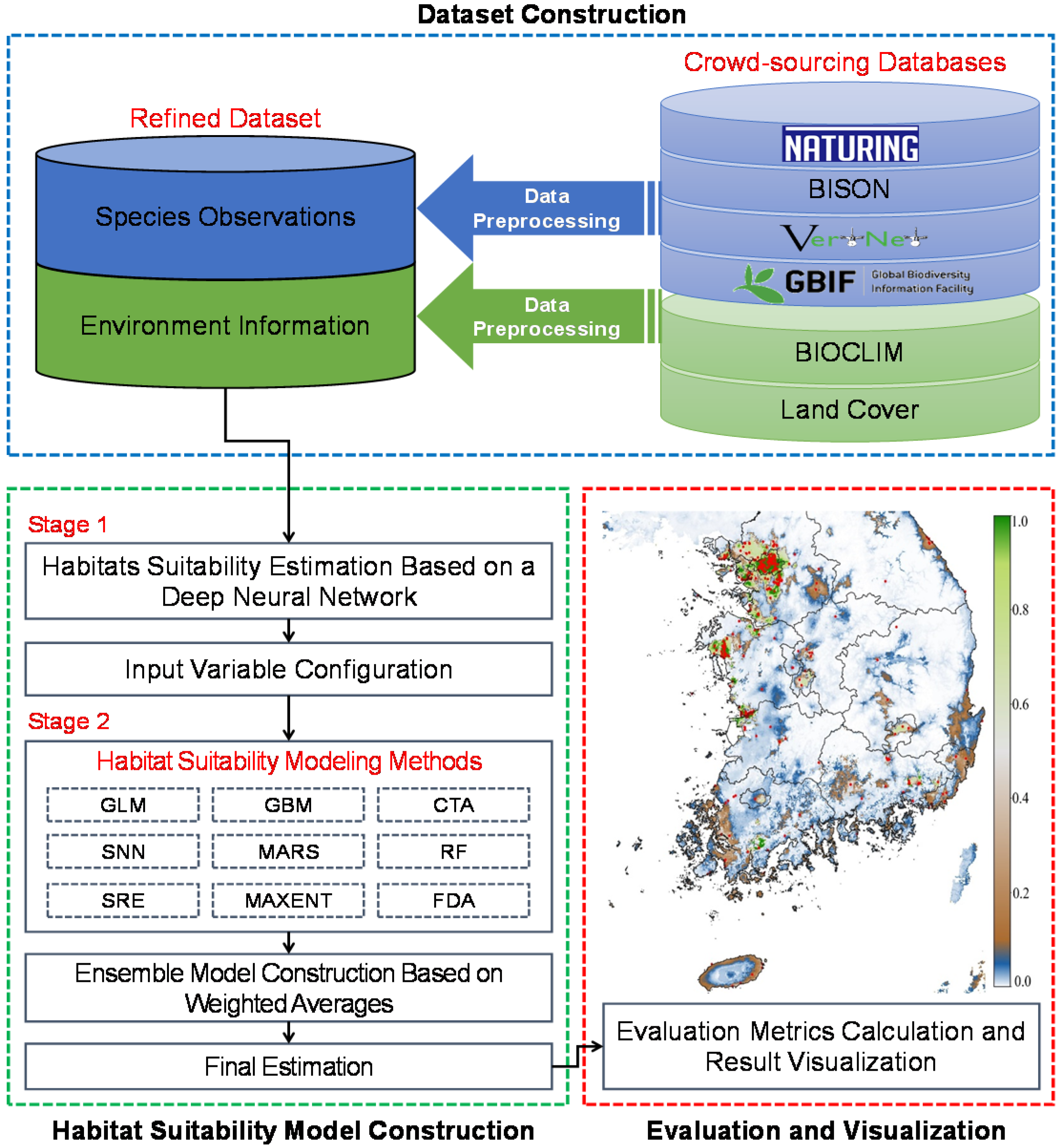
We describe in detail our two-stage habitat suitability estimation model with the overall structure (Figure 1). Observational, global climatic [40], and Korean land cover data [41] were initially collected to configure the independent variables for our model. In the first stage of the model, we constructed a DNN model as a sub-model. Next, a stacking ensemble-based estimation model was constructed using the results of the DNN sub-model as input to improve estimation performance. Finally, the habitat suitability results and other widely used evaluation metrics, including area under the curve (AUC), sensitivity, specificity, the kappa statistic, and the TSS were visualized for a performance comparison between the TSEM and previously reported models [42,43,44,45,46,47].

2.2. Dataset Construction

In general, the performance of a DNN-based estimation model depends on the quality and size of the dataset used for training. To construct our dataset, we first reviewed several crowdsourced databases that contain global observations of various species, selected 11 target species that were primarily found in South Korea, and then collected observational data for these species. These species are all considered conservation targets in Korean wildlife conservation projects. We listed the target species and their number of observations, as reported in the global biodiversity information facility (GBIF), VertNet, biodiversity information serving our nation (BISON), and Naturing databases (

Table 2. Target species and their observations.

Target Species (Scientific Name)	Image	IUCN Red List	Number of Observations in South Korea	Suitable Habitats
Streptopelia orientalis		Least Concern	1523	Shrubland, Terrestrial, Forest
Passer montanus		Least Concern	1498	Shrubland, Terrestrial, Forest
Ardea cinerea		Least Concern	1116	Marine neritic, Forest, Wetlands, Grassland
Hypsipetes amaurotis		Least Concern	1162	Terrestrial, Forest
Hynobius leechii		Least Concern	1336	Wetlands, Forest
Anas zonorhyncha		Least Concern	856	Wetlands, Artificial/Aquatic and Marine, Terrestrial, Marine coastal
Rana huanrenensis		Least Concern	906	Wetlands, Forest, Grassland
Anas platyrhynchos		Least Concern	714	Wetlands, Artificial/Aquatic and Marine
Cyanopica cyanus		Least Concern	679	Forest, Terrestrial
Rana dybowskii		Least Concern	511	Wetlands, Aquatic and Marine, Terrestrial, Vegetation, Shrubland, Forest
Hyla japonica		Least Concern	1261	Wetlands, Aquatic and Marine, Terrestrial, Vegetation, Shrubland, Forest

). Species habitats are closely related to the climate and land conditions [42,43,44,45,46,47]. Therefore, to construct a valid habitat model, we collected various layers of environment information from Worldclim Bioclimatic [40] and a land cover dataset for South Korea [41], which are both widely used for ecological modeling. The land cover dataset for South Korea was generated using Korea multi-purpose satellite No. 2, also known as KOMPSAT No. 2 or Arirang 2, and satellite pour l’observation de la terre 5 (SPOT 5) remote sensing images from 2009. KOMPSAT No. 2, which is equipped with a 1-m high-resolution multi-spectral camera (MSC), has orbited Earth approximately 46,800 times in nine years, capturing approximately 75,400 high-quality satellite images of Korea, while SPOT 5 can capture satellite images with a coverage of 60 km × 60 km and a resolution of 5 m. Compared to the GlobCover, the land cover dataset for South Korea provides more detailed information due to its higher resolution. Because this land cover dataset consists of categorical variables, we converted them into proximity distance layers, which have continuous values. Proximity distance for land cover layers is regarded as crucial for modeling because the unique survival traits of species and their habitat characteristics are closely related. Indeed, several studies have improved the performance of habitat suitability estimation models by considering the distance between the environmental layers and species observations. For this reason, we also employed proximity distance as an input variable. In total, we used 41 environmental layers as input variables for our habitat suitability modeling (

Table 3. List of input variables.

Variable Name	Description	Type
BIO_1	Annual mean temperature	Continuous
BIO_2	Mean diurnal range	Continuous
BIO_3	Isothermality	Continuous
BIO_4	Temperature seasonality	Continuous
BIO_5	Max. temperature of the warmest month	Continuous
BIO_6	Min. temperature of the coldest month	Continuous
BIO_7	Temperature annual range	Continuous
BIO_8	Mean temperature of the wettest quarter	Continuous
BIO_9	Mean temperature of the driest quarter	Continuous
BIO_10	Mean temperature of the warmest quarter	Continuous
BIO_11	Mean temperature of the coldest quarter	Continuous
BIO_12	Annual precipitation	Continuous
BIO_13	Precipitation of the wettest month	Continuous
BIO_14	Precipitation of the driest month	Continuous
BIO_15	Precipitation seasonality	Continuous
BIO_16	Precipitation of the wettest quarter	Continuous
BIO_17	Precipitation of the driest quarter	Continuous
BIO_18	Precipitation of the warmest quarter	Continuous
BIO_19	Precipitation of the coldest quarter	Continuous
Distance_1	Proximity distance from each cell to a residential area (detached residential and common residential areas)	Continuous
Distance_2	Proximity distance from each cell to an industrial area	Continuous
Distance_3	Proximity distance from each cell to a commercial area (commercial/business and mixed residential/business areas)	Continuous
Distance_4	Proximity distance from each cell to a leisure facility area	Continuous
Distance_5	Proximity distance from each cell to a transportation area (airport, harbor, railway, road, and other transportation and communication facilities)	Continuous
Distance_6	Proximity distance from each cell to a public facility area (basic environmental, education/administrative, and other public facilities)	Continuous
Distance_7	Proximity distance from each cell to paddy fields (land consolidation success and undergoing land consolidation in paddy fields)	Continuous
Distance_8	Proximity distance from each cell to dry fields (land consolidation success and undergoing land consolidation in dry fields)	Continuous
Distance_9	Proximity distance from each cell to a greenhouse	Continuous
Distance_10	Proximity distance from each cell to an orchard	Continuous
Distance_11	Proximity distance from each cell to other plantations (pastureland and other plantations)	Continuous
Distance_12	Proximity distance from each cell to broadleaf forest	Continuous
Distance_13	Proximity distance from each cell to coniferous forest	Continuous
Distance_14	Proximity distance from each cell to mixed forest	Continuous
Distance_15	Proximity distance from each cell to natural pasture	Continuous
Distance_16	Proximity distance from each cell to artificial pasture (golf course, cemetery, and other pastures)	Continuous
Distance_17	Proximity distance from each cell to inland wetland	Continuous
Distance_18	Proximity distance from each cell to coastal wetland (tidal mudflat and saltern)	Continuous
Distance_19	Proximity distance from each cell to naturally barren areas (beaches, riverbanks, and rocks)	Continuous
Distance_20	Proximity distance from each cell to artificially barren areas (mining area, playground, and other barrens)	Continuous
Distance_21	Proximity distance from each cell to inland water (rivers and lakes)	Continuous
Distance_22	Proximity distance from each cell to ocean water	Continuous

).

2.3. Data Preprocessing

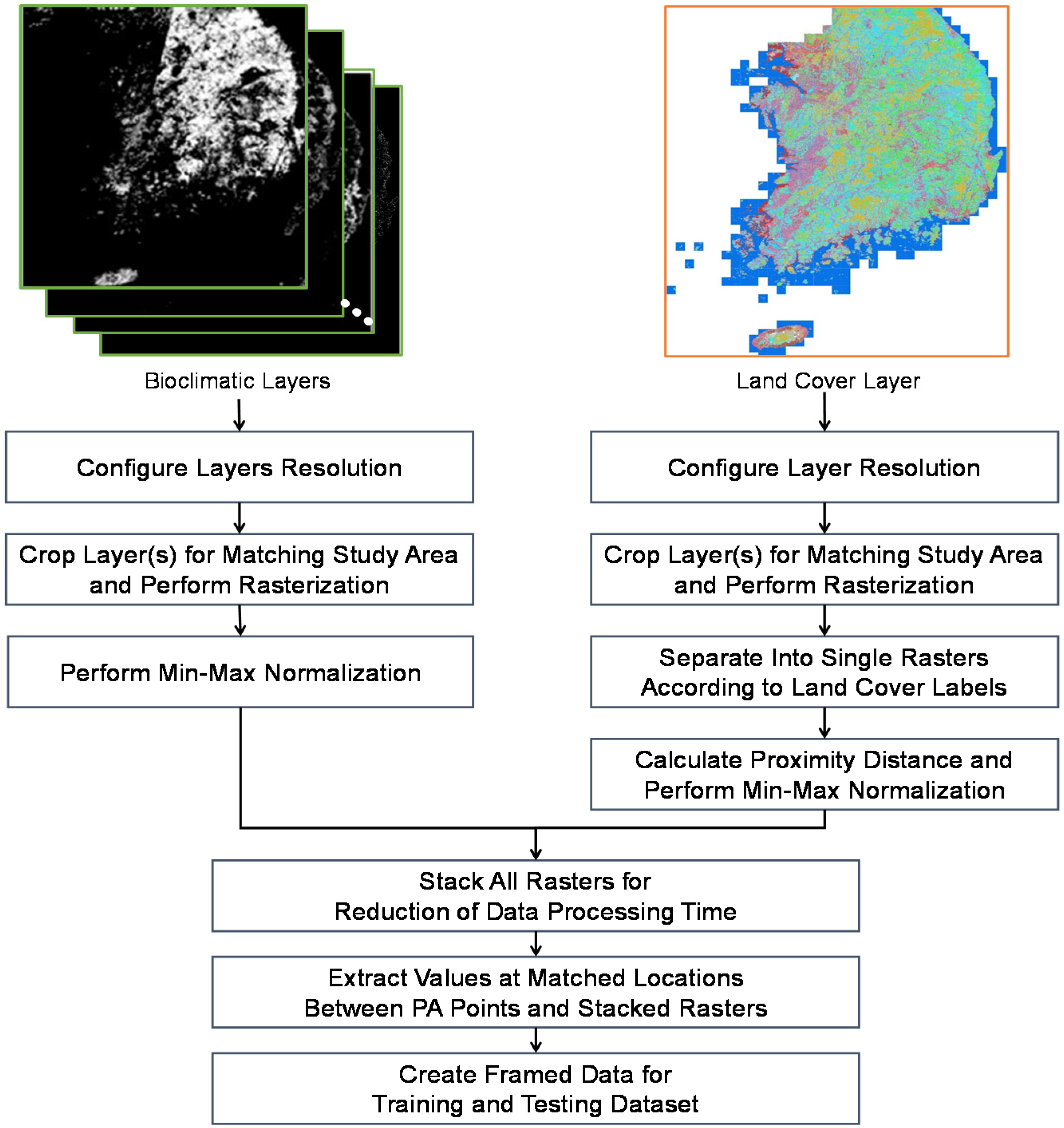
To conduct habitat suitability estimation, preprocessing of the collected observation data and environmental variables was required, consisting of a number of steps. We carried out this data preprocessing using Quantum Geographic Information System (QGIS) 3.8.1. We present the steps used to prepare the training and testing datasets in Figure 2. First, we set the resolution to 3000 × 3000 pixels and cropped the collected layers based on the study area, which corresponded to a rectangle on the map. For this, we used the World Geodetic System 1984 (WGS84), which is an Earth-centered, Earth-fixed terrestrial reference system and a geodetic datum. In this system, the entire South Korea region is represented by the latitude and longitude coordinates (125.000, 38.083), (129.583, 38.083), (125.000, 33.166), and (129.583, 33.166). Because the bioclimatic and land cover layers (i.e., the classified land cover in South Korea) are all in a shape (.shp) file format, we converted them into a gridded data (.grd) file format, which consists of scalar values on a regular rectangular grid, either in longitude or latitude space.

We configured each pixel of the raster to have a coverage of approximately 135 m, which produces 900 M grids if we convert the entire South Korean region into a grid space. We then applied min-max normalization to all variables in the cropped bioclimatic layers. For the preprocessing of the land cover layer, we first divided it into multiple layers according to the land cover labels and conducted rasterization. We then calculated the proximity distance based on the separate single rasters and applied min-max normalization to each distance raster. Finally, we stacked all of the rasters to generate a data frame that included labeled presence and absence, and that matched the values of the environmental rasters in the given presence and absence locations.

2.4. Stage 1: Habitat Suitability Estimation Based on a DNN

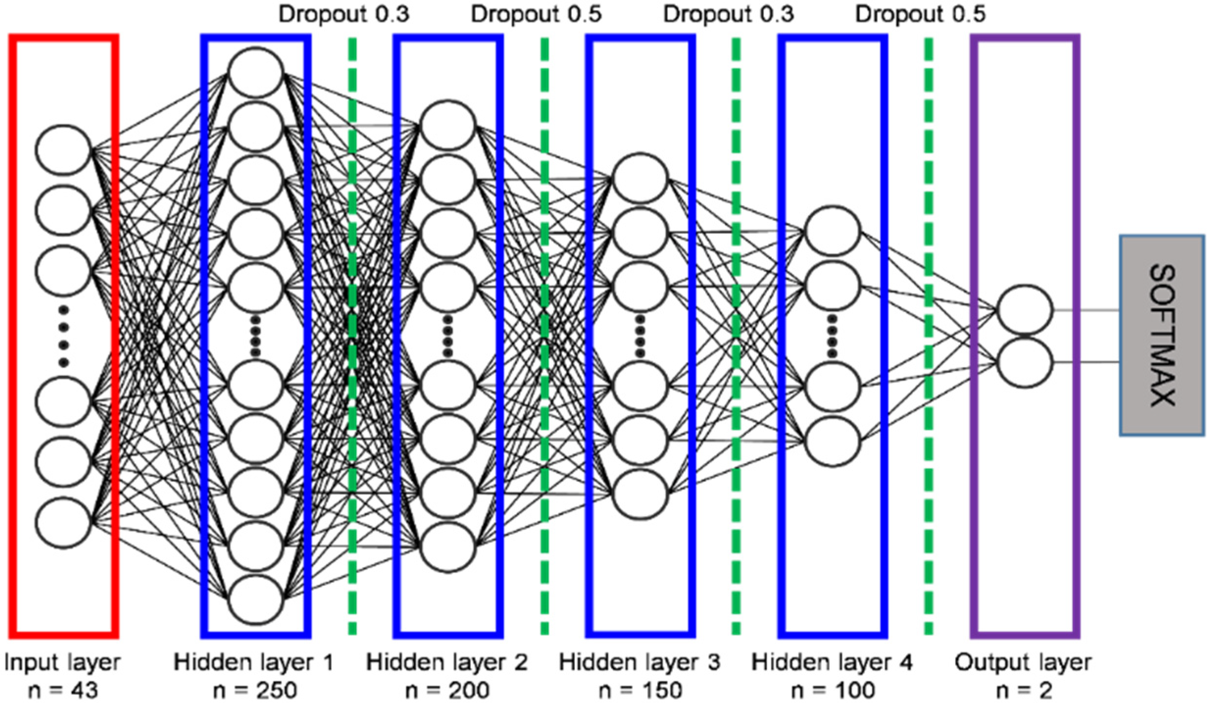
Recently, several DNN-based habitat suitability models have been proposed and have performed well when compared with previous methods [28,29,30]. Hence, we constructed a DNN model in the first stage to determine the probability of a species’ presence or absence, with a higher probability of presence for a species indicating higher habitat suitability. In general, DNNs consist of three types of layers: an input layer, one or more hidden layers, and an output layer. The input layer receives input variables, while the hidden layers are involved in hidden feature processing. The output layer then produces the final prediction. The prediction performance of a DNN model is determined by the configuration of each layer and the model design. For example, it has been shown that the learning rate, the optimizer, regularization, and the activation function significantly affect prediction performance [33]. To obtain the best performance from the DNN model, we carefully determined the optimal hyperparameters using grid search and considering related research [28]. We used the GridSearchCV function of the scikit-learn library [48]. The number of repetitions of grid search was set to infinite, and the number of cross-validations was set to five times. Consequently, when we constructed our DNN model, we used four hidden layers containing 250, 200, 150, and 100 neurons (Figure 3). We set the batch size to 75 and the number of epochs to 5000 with early stopping to optimize model training. To decide the batch size in the training stage, we carefully considered the results of the grid search. For training optimization, we tested three optimizers, including the stochastic gradient descent (SGD), root mean square propagation (RMSprop), adaptive moment estimation (ADAM), and then selected the ADAM as the best optimizer. In addition, we utilized the he-normal (HE) initialization to sort initial weights for individual inputs in a neuron model. The activation function controls the non-linearity of individual neurons. We tested five popular activation functions: linear, soft-max, rectified linear unit (ReLU), tangent, and sigmoid. Through the grid search, we selected ReLU as the activation function of our training model. The learning rate is a hyper-parameter that controls how much we are adjusting the weights of our network with respect to the loss gradient. If the learning rate is set too small, it might take a long time to converge on the performance goal. On the contrary, if the learning rate is set too large, the average loss will increase. To obtain the optimal learning rate, we performed a grid search with ADAM as the optimizer and ReLU as the activation function. Our training model was able to achieve optimal learning efficiency when the learning rate was 0.001.

The finished DNN model was to generate the probability of both presence and absence for a species. The more suitable an area was as habitat for a particular species, the closer the probability of that species’ presence was to 1, while the probability of absence followed the opposite trend.

2.5. Stage 2: Ensemble-Based Habitat Suitability Estimation

Ensembles of machine-learning techniques have been widely adopted to solve various prediction problems in past research [43,44,45,46,47]. Compared to one machine-learning model, ensembles can improve prediction performance by combining several models. In the field of ecological modeling, ensemble models are widely known as a useful approach for the construction of potential habitat estimation models [43,44,45,46,47]. Therefore, in the second stage, we developed an ensemble-based habitat suitability estimation model using the BIOMOD2 package [49] for R programming. We present the overall construction process for our ensemble model in Stage 2 in Figure 4.

According to the authors of [28,50], a low number of observations (i.e., n < 100) can degrade the estimation performance of a habitat model because using very few observations in model construction leads to overfitting and bias [8,9,10]. To solve this issue, we used 41 environmental layers and the results of habitat suitability from the DNN in Stage 1 as input variables for the ensemble model in Stage 2. This modeling method is known as stacking and can effectively avoid the possibility of overfitting and bias [51]. We built our ensemble model by combining GLM, GBM, CTA, SNN, FDA, MARS, RF, the SRE model, and MAXENT and used a weighted-average algorithm, which returns a weighted value for each model based on selected evaluation scores. Therefore, an accurate estimation model will have a relatively high weighted value when it combines all of the models. Because the TSS has been proven to be a reliable evaluation metric when measuring and assessing the performance of habitat models [47], we used the TSS to calculate the weighted value. Equation (1) was used to calculate the final estimation using the weighted average value for each model, in which $i$ and $j$ represent the class label for presence and absence and the number of models, respectively, $\widehat{y}$ indicates the estimated class label, and $p_{ij}$ is the calculated probability of the $j$th model. In addition, $w_j$ is the weighted value of the $j$th model, which was calculated using Equation (2). We evaluated each model using five-fold cross-validation and obtained the final TSS value as the average of the TSSs generated by the individual models.

$$\widehat{y}=\underset{i}{argmax}{\displaystyle \sum }_{j=1}^m{w}_j\ast p_{ij}$$

(1)

$$w_j=\frac{TS{S}_j-Min\left(TSS\right)}{Max\left(TSS\right)-Min\left(TSS\right)}$$

(2)

3. Results and Discussion

We evaluated our proposed model and compared its performance with other approaches to habitat suitability modeling. We first explained the evaluation metrics used to assess the quality of habitat suitability estimation and then evaluated the performance of our proposed model and other commonly used models using these metrics. We also visualized the results for habitat suitability analysis using map overlays.

3.1. Evaluation Metrics

To evaluate the performance of our model, we used five metrics: sensitivity, specificity, the kappa statistic, AUC, and TSS. These have all been regularly used to assess habitat modeling performance in ecology [47]. The percentage of correctly predicted sites was excluded as a measure of prediction accuracy for the proposed model because, even though it is simple to calculate, its usefulness is severely limited for rare species [19]. To evaluate the estimation results, we used a confusion matrix in which a, b, c, and d indicate true positive, false positive, false negative, and true negative, respectively (

Table 4. Confusion matrix for the evaluation of our presence–absence model.

Predicted	Observed
	Presence	Absence
Presence	a	b
Absence	b	d

). For instance, when the ground truth is the presence and the prediction result from the proposed model is also the presence, then we counted it as a true positive. Sensitivity, specificity, the kappa statistic, and TSS were calculated using Equations (3)–(6), respectively, based on this confusion matrix.

$$Sensitivity=\frac{a}{a+c}$$

(3)

$$Specificity=\frac{d}{b+d}$$

(4)

$$Kappa statistic=\frac{\left(\frac{a+d}{n}\right)-\frac{\left(a+c\right)\left(a+b\right)+\left(b+d\right)\left(c+d\right)}{n^2}}{1-\frac{\left(a+c\right)\left(a+b\right)+\left(b+d\right)\left(c+d\right)}{n^2}}$$

(5)

TSS = sensitivity + specificity − 1

(6)

Sensitivity represents the probability that a model will correctly predict the presence of a species, while specificity measures the probability of a model accurately predicting the absence of a species. TSS normalizes overall accuracy [47,50]. AUC is widely used to assess the accuracy of habitat suitability models because it is easy to interpret, thus allowing comparison between models. ROC curves are frequently used as a single threshold-independent measure for model performance. In previous studies designed to predict habitat suitability [52,53,54], models with an AUC greater than 0.8 were considered valid as predictive models. The kappa statistic is also a common evaluation metric used for habitat suitability estimation models, but it has been criticized for being heavily dependent on prevalence. TSS, on the other hand, avoids this problem while offering the advantages of the kappa statistic. In general, most ecological modeling research uses sensitivity, specificity, the kappa statistic, and TSS together to analyze the performance of habitat suitability models [51,52,53,54,55]. Thus, we used these five metrics together to compare their weaknesses, strengths, and commonalities.

3.2. Performance Evaluation

We described the comparison results for the habitat suitability models using the five metrics discussed in Section 3.1. We compared as many estimation models as possible, including GLM, GBM, CTA, SNN, FDA, MARS, RF, SRE, DNN, ensemble models not including DNN (EMED), and our proposed approach. As mentioned above, EMED has demonstrated satisfactory performance in the previous studies. We constructed the EMED model in the present study using GLM, GBM, CTA, SNN, FDA, MARS, RF, and SRE. All of these models were trained and tested using the BIOMOD2 package in R and were verified using five-fold cross-validation. We used 80% of the species observation as the training set and 20% as the test set. We present the selected parameters and training strategies for each model in the following (

Table 5. Selected parameters and training strategies for the estimation models.

Estimation Model	Selected Parameters and Training Strategies
GLM	Quadratic-type regression Akaike information criterion (AIC) for environmental layer selection
GBM	Bernoulli distribution, 2500 trees, 7 depths, 5 terminal nodes, 0.001 learning rate
CTA	Categorical classification, Default tree parameter (auto-optimized by BIOMOD2)
SNN	Single hidden layer, Auto-optimized neuron size, 200 iterations
FDA	Mars method
MARS	Simple pricewise linear, 0.001 threshold, Backward pruning method
RF	Maximum of 500 trees, Default number of variables at each split (auto-optimized by BIOMOD2), 5 nodes
SRE	0.025 quantile for environmental variable selection
MAXENT	Maximum of 200 iterations, Linear and quadratic variables Default parameters for threshold and hinge (auto-optimized by BIOMOD2)
EMED	Assigning weights using TSS evaluation, Weighted average-based model assembly, 0.7 for the ensemble threshold, Committee averaging

).

We calculated the estimation performance of various models for target species using five metrics and present their averages in

Table 6. Performance comparison of estimation models.

Estimation Model	Evaluation Metrics (Avg.)
	Sensitivity	Specificity	AUC	Kappa Statistic	TSS
GLM	0.855	0.833	0.888	0.662	0.689
GBM	0.879	0.906	0.950	0.780	0.785
CTA	0.854	0.884	0.901	0.724	0.738
SNN	0.857	0.880	0.920	0.723	0.738
FDA	0.865	0.892	0.938	0.750	0.758
MARS	0.859	0.871	0.927	0.711	0.731
RF	0.885	0.947	0.967	0.838	0.832
SRE	0.567	0.904	0.735	0.499	0.470
MAXENT	0.781	0.816	0.862	0.665	0.658
DNN (Stage 1)	0.757	0.957	0.886	0.753	0.759
EMED	0.905	0.911	0.972	0.862	0.816
TSEM (Stage 2)	0.966	0.920	0.983	0.887	0.886

The highest values are in bold.

. Detailed experimental results, including sensitivity, specificity, AUC, kappa statistic, and TSS, can be found in the Supplementary Materials (Tables S1–S5). To objectively assess the estimation results, we show the evaluation criteria of AUC, kappa statistic, and TSS in

Table 7. Evaluation criteria of AUC, kappa statistic and TSS.

	AUC	Kappa Statistic	TSS
Excellent	$\ge 0.9$	$\ge 0.9$	$\ge 0.8$
Good	$0.8-0.9$	$0.8-0.9$	$0.6-0.8$
Fair	$0.6-0.8$	$0.7-0.8$	$0.4-0.6$
Poor or no predictive ability	$\le 0.6$	$\le 0.6$	$\le 0.4$

. We can observe that our proposed model showed the best performance, while the DNN exhibited weak performance because model training was insufficient due to the lack of training data. Likewise, the SRE model showed a poor performance for the prediction (AUC < 0.6). Even though the SRE model is intuitive and fast, it does not fully reflect the interactions between environmental conditions and species distributions in modeling. All other models except the DNN and SRE models performed reasonably well in terms of predicting the presence of a species. In contrast, in terms of specificity, DNN was the best performing model. The AUC has long been regarded as the standard metric for assessing the performance of habitat suitability models. In most cases, TSEM demonstrated the best estimation performance, while EMED also generated high AUC values, with an average of 0.972. This demonstrates that the two-stage based ensemble approach can improve estimation performance. While TSEM performed best for kappa statistic and TSS, SRE was the worst-performing model. For Hyla japonica, EMED yielded a higher TSS (EMED = 0.786 and TSEM = 0.783) than TSEM because the DNN model in the first stage produced very poor estimation results. However, for all other species, our model outperformed the other models. In summary, based on these comparisons, clearly TSEM is more suitable for deriving ecological insights related to habitat suitability estimation.

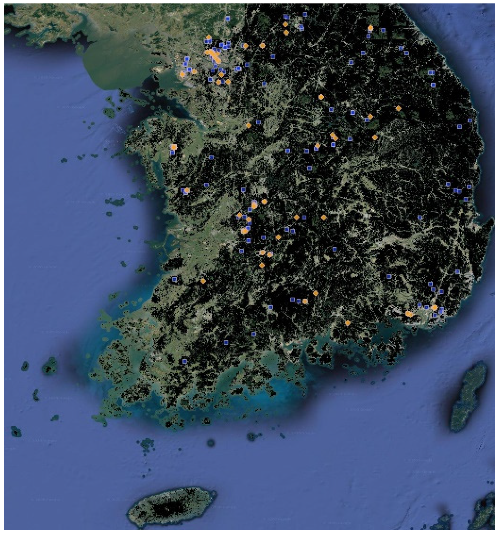
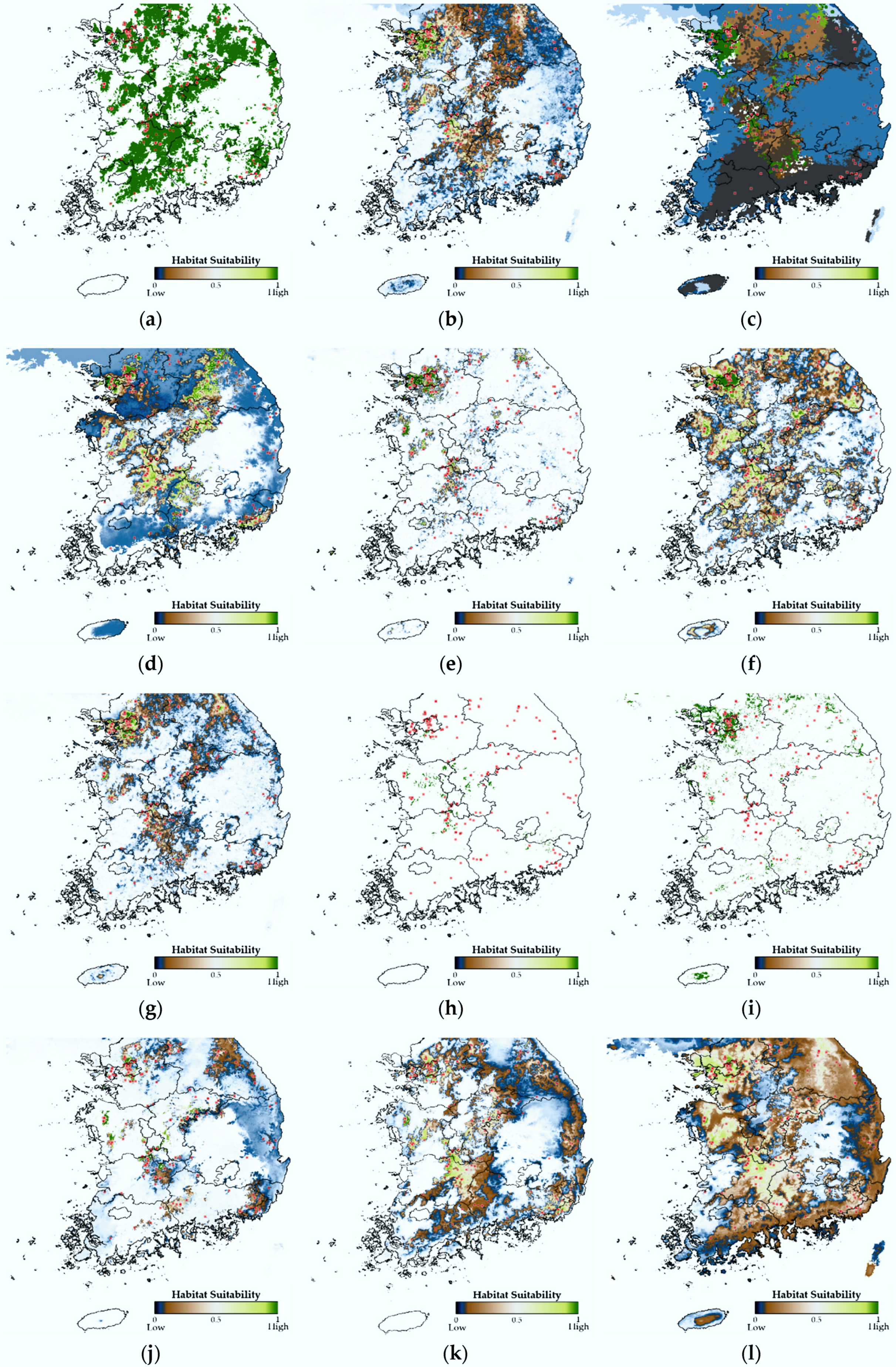
To confirm whether the estimation results of our model are valid, we selected Rana huanrenensis as a visualization case. The visualizations of the results for other target species can be found in the Supplementary Materials (Figures S1–S10). Rana huanrenensis, also known as the Korean stream brown frog, lives mainly in Korea and Japan, and its habitats are identified as wetland, forest, and grassland (Table 2). Due to the low number of confirmed populations of this species, it could be listed as vulnerable (VN) under the IUCN Red List criterion, but is listed as least concern (LC) based on the assumption of widespread occurrence, especially in Korea. The Rana huanrenensis lives in valleys in high montane regions, above 500 m in elevation [56]. This species is mainly observed from March to April, which is very closely related to the breeding season of this species. Rana huanrenensis breeds in slow-moving montane streams and rivers, and their eggs are laid in moderately small masses that are attached to submerged rocks [57]. Indeed, the distribution of observation data for Rana huanrenensis fits well with their habitat characteristics. We marked the blue points as a training set and yellow points as a test set. The areas marked in black represent the entire coniferous forest, mixed forest, and broad-leaved forest (Figure 5). In Figure 6, green indicates suitable species habitats and blue indicates uninhabitable areas. In evaluating the habitat suitability estimation of Rana huanrenensis, TSEM showed a better estimation performance (TSS = 0.949) than other estimation models. Although EMED and RF performed slightly worse than TSEM (TSS of EMED = 0.819 and TSS of RF = 0.822), these models showed excellent estimation performance based on evaluation criteria. The distribution of Rana huanrenensis habitat estimated by TSEM is very similar to the mountainous terrain of South Korea. The SNN, MARS, GBM, EMED, and RF also showed the distribution of habitat estimations similar to mountainous terrain. However, we confirmed that the MARS, GBM, EMED, and RF estimated that the Rana huanrenensis was suitable for habitation in some regions, including residential, industrial, and commercial areas. The TSEM estimated that the areas of mixed forests, coniferous forests, and broad-leaved forests were relatively more suitable as the Rana huanrenensis habitat. Even though the TSEM was trained and tested on crowdsourced datasets of the Rana huanrenensis, the estimation results matched well with their actual habitats because most of the observation data for the Rana huanrenensis were near the main habitats such as wetland, montane streams, and forest. We demonstrated that the habitat suitability results estimated by the TSEM are well-matched when compared with the existing studies of the Rana huanrenensis habitats [56,57].

3.3. Statistical Evaluation

To demonstrate the superiority of our proposed method, we performed Wilcoxon signed-rank and Friedman tests [58,59]. The Wilcoxon signed-rank test is a non-parametric statistical hypothesis test used to compare two related samples [58]. It can be used as an alternative to the t-test when one or more of the samples are not normally distributed. It establishes a null hypothesis to determine whether there is a significant difference between the two samples. If the p-value is less than a certain significance level, the null hypothesis is rejected, and the two samples are assumed to be significantly different. In the statistical hypothesis testing, the p-value is the probability of obtaining test results at least as extreme as the results actually observed during the test, assuming that the null hypothesis is correct. The Friedman test is a multiple comparison test that aims to identify significant differences between three or more samples [59]. It first ranks each row (block) together, and then considers the values of the ranks by column. The data are organized into a matrix with B rows (blocks) and T columns (treatments) with a single operation in each cell of the matrix. To verify the results of these tests, we used AUC, the kappa statistic, and TSS for each machine-learning method. The results of the Wilcoxon signed-rank test, for which the significance level was set to 0.05, and the Friedman test are listed in

Table 8. The results of the Wilcoxon signed-rank and Friedman tests for our proposed method.

Estimation Models	Wilcoxon Signed-Rank Test (p-Value < 0.05)			Friedman Test
	AUC	Kappa	TSS	AUC	Kappa	TSS
GLM	0.00098	0.00098	0.00098	$2.236\times {10}^{-17}$	$1.446\times {10}^{-18}$	$2.236\times {10}^{-17}$
GBM	0.00379	0.00098	0.00384
CTA	0.00384	0.00098	0.00384
SNN	0.00382	0.00098	0.00098
FDA	0.00098	0.00098	0.00382
MARS	0.00381	0.00382	0.00382
RF	0.00379	0.00384	0.00384
SRE	0.00379	0.00098	0.89390
MAXENT	0.00098	0.00098	0.00098
DNN (Stage 1)	0.00098	0.00098	0.00098
EMED	0.00368	0.00382	0.00195

AUC, area under the curve; Kappa, kappa statistic; TSS, true skill statistic.

. Based on these tests, our proposed method exhibited significantly better prediction performance than the other machine-learning methods because the p-value was below the significance level in most cases.

4. Conclusions

In this study, we focused on a two-stage modeling scheme that can be applied to habitat suitability estimation for various species. First, we investigated and selected 11 species that are present in South Korea and regarded as targets for species conservation research. To obtain a sufficient number of observations for the target species, we extracted observational data for these species from several crowdsourced databases and added them to our database. Since spatial bias is a well-known problem in crowdsourced data, we tried to alleviate this bias by using three global datasets and one domestic dataset. In particular, the domestic dataset, Naturing database, contains data of target species observed quite evenly across South Korea. We also employed 41 environmental layers that included information on the global climate and the land cover of South Korea as input variables. To effectively estimate habitat suitability, we used a DNN model and an ensemble of habitat suitability estimation models in the first and second stages, respectively. To evaluate the effectiveness of the proposed model, we compared it with previously employed models and visualized these results using a suitability map overlay. The experimental results demonstrate that the proposed model has significant potential for use in estimating habitat suitability.

For model training and testing, we used crowdsourced datasets. This implies that there could be some bias in the observation data and the estimation results, as mentioned above. Hence, even though our model showed better performance than other models, estimation results might indicate where the observation was made, in other words, the species can be observed. To the best of our knowledge, it is an inevitable limitation of prediction models based on crowdsourced data. In future work, to ensure the reliability of our habitat suitability model, we plan to develop a method that can alleviate the potential biases of crowdsourcing datasets.

References

- Pimm, S.L.; Russell, G.J.; Gittleman, J.L.; Brooks, T.M. The future of biodiversity. Science 1995, 269, 347–350. [Google Scholar] [CrossRef] [PubMed] [Green Version]
- Dirzo, R.; Raven, P.H. Global State of Biodiversity and Loss. Annu. Rev. Environ. Resour. 2003, 28, 137–167. [Google Scholar] [CrossRef] [Green Version]
- Jenkins, M. Prospects for Biodiversity. Science 2003, 302, 1175–1177. [Google Scholar] [CrossRef] [PubMed]
- Corsi, F.; Duprè, E.; Boitani, L. A large-scale model of wolf distribution in Italy for conservation planning. Conserv. Biol. 1999, 13, 150–159. [Google Scholar] [CrossRef]
- Peterson, A.T.; Soberón, J.; Sánchez-Cordero, V. Conservatism of ecological niches in evolutionary time. Science 1999, 285, 1265–1267. [Google Scholar] [CrossRef]
- Franklin, J. Species distribution models in conservation biogeography: Developments and challenges. Divers. Distrib. 2013, 19, 1217–1223. [Google Scholar] [CrossRef]
- Araújo, M.B.; Peterson, A.T. Uses and misuses of bioclimatic envelope modeling. Ecology 2012, 93, 1527–1539. [Google Scholar] [CrossRef] [Green Version]
- Heikkinen, R.K.; Luoto, M.; Araújo, M.B.; Virkkala, R.; Thuiller, W.; Sykes, M.T. Methods and uncertainties in bioclimatic envelope modelling under climate change. Prog. Phys. Geogr. 2006, 30, 751–777. [Google Scholar] [CrossRef] [Green Version]
- Thuiller, W.; Lafourcade, B.; Araujo, M. Presentation manual for BIOMOD. Ecography 2010, 32, 369–373. [Google Scholar] [CrossRef]
- Elith, J.; Graham, C.H.; Anderson, R.P.; Dudík, M.; Ferrier, S.; Guisan, A.; Hijmans, R.J.; Huettmann, F.; Leathwick, J.R.; Lehmann, A.; et al. Novel methods improve prediction of species’ distributions from occurrence data. Ecography 2006, 29, 129–151. [Google Scholar] [CrossRef] [Green Version]
- Leathwick, J.R.; Elith, J.; Hastie, T. Comparative performance of generalized additive models and multivariate adaptive regression splines for statistical modelling of species distributions. Ecol. Modell. 2006, 199, 188–196. [Google Scholar] [CrossRef]
- Zuur, A.F.; Ieno, E.N.; Elphick, C.S. A protocol for data exploration to avoid common statistical problems. Methods Ecol. Evol. 2010, 1, 3–14. [Google Scholar] [CrossRef]
- Friedman, J.H. Multivariate adaptive regression splines. Ann. Stat. 1991, 1–67. [Google Scholar] [CrossRef]
- Hastie, T.; Tibshirani, R.; Buja, A. Flexible discriminant analysis by optimal scoring. J. Am. Stat. Assoc. 1994, 89, 1255–1270. [Google Scholar] [CrossRef]
- Phillips, N.D.; Reid, N.; Thys, T.; Harrod, C.; Payne, N.L.; Morgan, C.A.; White, H.J.; Porter, S.; Houghton, J.D.R. Applying species distribution modelling to a data poor, pelagic fish complex: The ocean sunfishes. J. Biogeogr. 2017, 44, 2176–2187. [Google Scholar] [CrossRef]
- Reiss, H.; Cunze, H.; König, K.; Neumann, K.; Kröncke, I. Species distribution modelling of marine benthos: A North Sea case study. Mar. Ecol. Prog. Ser. 2011, 442, 71–86. [Google Scholar] [CrossRef] [Green Version]
- Guisan, A.; Thuiller, W. Predicting species distribution: Offering more than simple habitat models. Ecol. Lett. 2005, 8, 993–1009. [Google Scholar] [CrossRef]
- Phillips, S.J.; Anderson, R.P.; Schapire, R.E. Maximum entropy modeling of species geographic distributions. Ecol. Model. 2006, 190, 231–259. [Google Scholar] [CrossRef] [Green Version]
- Heikkinen, R.K.; Luoto, M.; Kuussaari, M.; Toivonen, T. Modelling the spatial distribution of a threatened butterfly: Impacts of scale and statistical technique. Landsc. Urban Plan. 2007, 79, 347–357. [Google Scholar] [CrossRef]
- Thomaes, A.; Kervyn, T.; Maes, D. Applying species distribution modelling for the conservation of the threatened saproxylic Stag Beetle (Lucanus cervus). Biol. Conserv. 2008, 141, 1400–1410. [Google Scholar] [CrossRef]
- De’ath, G.; Fabricius, K.E. Classification and regression trees: A powerful yet simple technique for ecological data analysis. Ecol. Lett. 2000, 81, 3178–3192. [Google Scholar] [CrossRef]
- Breiman, L.; Friedman, J.; Stone, C.J.; Olshen, R.A. Classification and regression trees; CRC press: Boca Raton, FL, USA, 1984. [Google Scholar] [CrossRef]
- De’Ath, G. Boosted trees for ecological modeling and prediction. Ecol. Lett. 2007, 88, 243–251. [Google Scholar] [CrossRef]
- D’heygere, T.; Goethals, P.L.; De Pauw, N. Genetic algorithms for optimisation of predictive ecosystems models based on decision trees and neural networks. Ecol. Model. 2006, 195, 20–29. [Google Scholar] [CrossRef]
- Fukuda, S.; De Baets, B.; Waegeman, W.; Verwaeren, J.; Mouton, A.M. Habitat prediction and knowledge extraction for spawning European grayling (Thymallus thymallus L.) using a broad range of species distribution models. Environ. Model. Softw. 2013, 47, 1–6. [Google Scholar] [CrossRef]
- Breiman, L. Random forests. Mach. Learn. 2001, 45, 5–32. [Google Scholar] [CrossRef] [Green Version]
- Cutler, D.R.; Edwards, T.C., Jr.; Beard, K.H.; Cutler, A.; Hess, K.T.; Gibson, J.; Lawler, J.J. Random forests for classification in ecology. Ecology 2007, 88, 2783–2792. [Google Scholar] [CrossRef]
- Rademaker, M.; Hogeweg, L.; Vos, R. Modelling the niches of wild and domesticated Ungulate species using deep learning. BioRxiv 2019, 744441. [Google Scholar] [CrossRef]
- Botella, C.; Joly, A.; Bonnet, P.; Monestiez, P.; Munoz, F. A deep learning approach to species distribution modelling. In Multimedia Tools and Applications for Environmental & Biodiversity Informatics; Springer: Cham, Switzerland, 2018; pp. 169–199. [Google Scholar] [CrossRef] [Green Version]
- Hulleman, W.; Vos, R.A. Modeling abiotic niches of crops and wild ancestors using deep learning: A generalized approach. BioRxiv 2019, 826347. [Google Scholar] [CrossRef]
- Rew, J.; Park, S.; Cho, Y.; Jung, S.; Hwang, E. Animal movement prediction based on predictive recurrent neural network. Sensors 2019, 19, 4411. [Google Scholar] [CrossRef] [Green Version]
- Moon, J.; Park, S.; Rho, S.; Hwang, E. A comparative analysis of artificial neural network architectures for building energy consumption forecasting. Int. J. Distrib. Sens. Netw. 2019, 15. [Google Scholar] [CrossRef] [Green Version]
- Moon, J.; Kim, Y.; Son, M.; Hwang, E. Hybrid Short-Term Load Forecasting Scheme Using Random Forest and Multilayer Perceptron. Energies 2018, 11, 3283. [Google Scholar] [CrossRef] [Green Version]
- Kim, H.; Kim, H.; Hwang, E. Real-time facial feature extraction scheme using cascaded networks. In Proceedings of the IEEE International Conference on Big Data and Smart Computing (BigComp), Kyoto, Japan, 27 February–2 March 2019; pp. 1–7. [Google Scholar] [CrossRef]
- Kim, J.; Moon, J.; Hwang, E.; Kang, P. Recurrent inception convolution neural network for multi short-term load forecasting. Energy Build. 2019, 194, 328–341. [Google Scholar] [CrossRef]
- GBIF Homepage. Available online: https://www.gbif.org (accessed on 5 March 2020).
- VertNet Homepage. Available online: http://vertnet.org (accessed on 5 March 2020).
- BISON Homepage. Available online: https://bison.usgs.gov (accessed on 5 March 2020).
- Naturing Homepage. Available online: https://www.naturing.net (accessed on 5 March 2020).
- Worldclim Homepage. Available online: https://www.worldclim.org (accessed on 5 March 2020).
- Land Cover of South Korea Homepage. Available online: http://www.neins.go.kr/gis/mnu01/doc03a.asp (accessed on 5 March 2020).
- Ferraz, K.M.P.M.d.B.; Ferraz, S.F.d.B.; Paula, R.C.d.; Beisiegel, B.; Breitenmoser, C. Species distribution modeling for conservation purposes. Nat. Conserv. 2012, 10, 214–220. [Google Scholar] [CrossRef] [Green Version]
- Wan, J.; Wang, C.; Han, S.; Yu, J. Planning the priority protected areas of endangered orchid species in northeastern China. Biodivers. Conserv. 2014, 23, 1395–1409. [Google Scholar] [CrossRef]
- Buisson, L.; Thuiller, W.; Casajus, N.; Lek, S.; Grenouillet, G. Uncertainty in ensemble forecasting of species distribution. Glob. Change Biol. 2010, 16, 1145–1157. [Google Scholar] [CrossRef]
- Forester, B.R.; DeChaine, E.G.; Bunn, A.G. Integrating ensemble species distribution modelling and statistical phylogeography to inform projections of climate change impacts on species distributions. Divers. Distrib. 2013, 19, 1480–1495. [Google Scholar] [CrossRef]
- Ranjitkar, S.; Xu, J.; Shrestha, K.K.; Kindt, R. Ensemble forecast of climate suitability for the Trans-Himalayan Nyctaginaceae species. Ecol. Model. 2014, 282, 18–24. [Google Scholar] [CrossRef]
- Allouche, O.; Tsoar, A.; Kadmon, R. Assessing the accuracy of species distribution models: Prevalence, kappa and the true skill statistic (TSS). J. Appl. Ecol. 2006, 43, 1223–1232. [Google Scholar] [CrossRef]
- Sckit-learn Homepage. Available online: https://https://scikit-learn.org/stable (accessed on 5 March 2020).
- Thuiller, W.; Lafourcade, B.; Engler, R.; Araújo, M.B. BIOMOD–a platform for ensemble forecasting of species distributions. Ecography 2009, 32, 369–373. [Google Scholar] [CrossRef]
- Miller, J. Species distribution modeling. Geogr. Compass 2010, 4, 490–509. [Google Scholar] [CrossRef]
- Moon, J.; Jung, S.; Rew, J.; Rho, S.; Hwang, E. Combination of short-term load forecasting models based on a stacking ensemble approach. Energy Build. 2020, 216, 109921. [Google Scholar] [CrossRef]
- Thuiller, W.; Araújo, M.B.; Lavorel, S. Generalized models vs. classification tree analysis: Predicting spatial distributions of plant species at different scales. J. Veg. Sci. 2003, 14, 669–680. [Google Scholar] [CrossRef]
- Giannini, T.C.; Chapman, D.S.; Saraiva, A.M.; Alves-dos-Santos, I.; Biesmeijer, J.C. Improving species distribution models using biotic interactions: A case study of parasites, pollinators and plants. Ecography 2013, 36, 649–656. [Google Scholar] [CrossRef] [Green Version]
- Barbet-Massin, M.; Jetz, W. A 40-year, continent-wide, multispecies assessment of relevant climate predictors for species distribution modelling. Divers. Distrib. 2014, 20, 1285–1295. [Google Scholar] [CrossRef]
- Duque-Lazo, J.; van Gils, H.; Groen, T.A.; Navarro-Cerrillo, R.M. Transferability of species distribution models: The case of Phytophthora cinnamomi in Southwest Spain and Southwest Australia. Ecol. Modell. 2016, 320, 62–70. [Google Scholar] [CrossRef]
- Liu, M.; Liu, Y.; Li, J. Reproductive habits of Rana huanrenensis. Sichuan J. Zool. 2004, 23, 183–184. [Google Scholar]
- Yang, S.Y.; Kim, J.B.; Min, M.S.; Suh, J.H.; Kang, Y.J.; Matsui, M.; Fei, L. First record of a brown frog Rana huanrenensis (Family Ranidae) from Korea. Korean J. Biol. Sci. 2000, 4, 45–50. [Google Scholar] [CrossRef]
- Park, S.; Moon, J.; Jung, S.; Rho, S.; Baik, S.W.; Hwang, E. A two-stage industrial load forecasting scheme for day-ahead combined cooling, heating and power scheduling. Energies 2020, 13, 443. [Google Scholar] [CrossRef] [Green Version]
- Moon, J.; Kim, J.; Kang, P.; Hwang, E. Solving the Cold-Start Problem in Short-Term Load Forecasting Using Tree-Based Methods. Energies 2020, 13, 886. [Google Scholar] [CrossRef] [Green Version]
Figure 1.
Overall process of the TSEM.
Figure 2.
The overall preprocessing process for the present study.
Figure 3.
Construction of the DNN model used in Stage 1 of the present study.
Figure 4.
Construction of the ensemble model employed in Stage 2 of the present study.
Figure 5.
Observations of Rana huanrenensis in South Korea.
Figure 6.
Habitat suitability visualization of Rana huanrenensis–(a) GLM; (b) GBM; (c) CTA; (d) SNN; (e) FDA; (f) MARS; (g) RF; (h) SRE; (i) MAXENT; (j) DNN; (k) EMED; (l) TSEM.