Ice Production in Ross Ice Shelf Polynyas during 2017–2018 from Sentinel–1 SAR Images


1
Key Laboratory of Remote Sensing of Gansu Province, Heihe Remote Sensing Experimental Research Station, Cold and Arid Regions Environmental and Engineering Research Institute, Chinese Academy of Sciences, Lanzhou 730000, China
2
Laboratory for Remote Sensing and Geoinformatics, Department of Geological Sciences, University of Texas at San Antonio, San Antonio, TX 78249, USA
3
Center for Advanced Measurements in Extreme Environments, University of Texas at San Antonio, San Antonio, TX 78249, USA
*
Author to whom correspondence should be addressed.
Remote Sens. 2020, 12(9), 1484; https://0-doi-org.brum.beds.ac.uk/10.3390/rs12091484
Submission received: 21 April 2020
/
Revised: 30 April 2020
/
Accepted: 5 May 2020
/
Published: 7 May 2020
(This article belongs to the Special Issue Remote Sensing in Sea Ice)
Abstract
:High sea ice production (SIP) generates high-salinity water, thus, influencing the global thermohaline circulation. Estimation from passive microwave data and heat flux models have indicated that the Ross Ice Shelf polynya (RISP) may be the highest SIP region in the Southern Oceans. However, the coarse spatial resolution of passive microwave data limited the accuracy of these estimates. The Sentinel-1 Synthetic Aperture Radar dataset with high spatial and temporal resolution provides an unprecedented opportunity to more accurately distinguish both polynya area/extent and occurrence. In this study, the SIPs of RISP and McMurdo Sound polynya (MSP) from 1 March–30 November 2017 and 2018 are calculated based on Sentinel-1 SAR data (for area/extent) and AMSR2 data (for ice thickness). The results show that the wind-driven polynyas in these two years occurred from the middle of March to the middle of November, and the occurrence frequency in 2017 was 90, less than 114 in 2018. However, the annual mean cumulative SIP area and volume in 2017 were similar to (or slightly larger than) those in 2018. The average annual cumulative polynya area and ice volume of these two years were 1,040,213 km2 and 184 km3 for the RSIP, and 90,505 km2 and 16 km3 for the MSP, respectively. This annual cumulative SIP (volume) is only 1/3–2/3 of those obtained using the previous methods, implying that ice production in the Ross Sea might have been significantly overestimated in the past and deserves further investigations.
1. Introduction
Coastal polynyas are common features during autumn and winter in polar regions and are dominantly caused by katabatic winds [1,2,3,4]. The ice forming in coastal polynyas due to low air/water temperature and the consequent brine rejection increases the salinity of the near-surface layer water [5,6,7]. As the next wind blows away the just formed new ice in polynyas, a subsequent set of new ice forms, leading to further brine rejection. This process of new ice formation occurs frequently as long as the katabatic wind occurs frequently in polar regions. Coastal polynyas are therefore regarded as the factories of sea ice production (SIP) [8,9,10]. This high SIP in polar regions causes high-salinity water; the sinking of this dense water drives the global thermohaline circulation [11,12,13,14,15] and also impacts the bio–related material cycle and ecosystem [16,17].
Many studies have been performed to quantitatively estimate polynya extent (area) and polynya ice production in coastal polynyas [12,18,19,20,21,22,23,24,25,26] and to analyze the relationship between sea ice production and dense deep-water formation [27,28]. Among them, Tamura et al. first mapped the SIP in the Southern Ocean [8], and then Tamura and Ohshima mapped SIP over the Arctic Ocean [23]. They reported that the highest ice production occurs in the RISP region with a mean annual cumulative SIP of 390 ± 59 km3 from the 1990s to 2000s. This is consistent with the fact that Antarctic Bottom Water (AABW) with the highest salinity is formed in the Ross Sea [13].
In the Ross Sea, the development and variability of polynyas are primarily caused by southerly airflow and associated katabatic winds from the Ross Ice Shelf and the higher elevation of the Antarctic continent [3,4]. It was reported that approximately 60% of the polynya events are linked to katabatic wind events; the remaining 40% are due to katabatic drainage winds and barrier winds that flow northward along the Transantarctic Mountains [2]. A summary of previous estimates of time–series of coastal polynya ice production in the Ross Sea is provided in Table 1. There are typically three polynyas in the Ross Sea: RISP, McMurdo Sound polynya (MSP), and Terra Nova Bay polynya (TNBP). Among previous studies, some regarded the RISP and MSP as one single polynya as Ross Sea Polynya (RSP), analyzing their combined ice production. The ice productions estimated by these studies show different results in the RSP. The long-term RSP ice productions (in Table 1) were all estimated based on the satellite passive microwave remote sensing (PMW) data and heat flux model. PMW data was used to derive ice thickness (of thin ice) and ice concentration and the heat flux model was used to calculate ice production based on the thin ice area (ice thickness <20 cm or sea ice concentration <75%). PMW is independent of sunlight, thus it is not affected by polar nights. Due to the strong penetrability of microwaves, PMW radiation can penetrate through the cloud cover. Therefore, the PMW data are available year-round at all weather conditions with a repeat cycle of half a day, and it is currently the longest dataset. The time series of satellite PMW data began in 1978, including the Scanning Multichannel Microwave Radiometer (SMMR, 1978–1987), the Special Sensor Microwave/Imager (SSM/I, 1987–2008), the Special Sensor Microwave Imager/Sounder (SSMI/S, 2007– ), and the Advanced Microwave Scanning Radiometer for EOS (AMSR-E) and AMSR2 (2002– ). The frequencies of these sensors are different but they all include K and Ka bands which have been used for ice thickness derivation. Due to power constraints, the SMMR was operated every second day; thus, real repeat time of SMMR was longer than that of SSM/I, SSMI/S, and AMSR-E. Therefore, after 1987 when the SSM/I(s) on DMSP satellite series began service, the temporal resolution of PMW data improved. Since 2002, AMSR-E on Aqua greatly improved the spatial resolution with the footprints of K and Ka bands of 16 × 27 km2 and 8.8 × 14.4 km2, respectively, enabling the identification of some smaller polynyas that could not be detected by SSM/I (s) [19]. Optical or thermal remote sensing are good choices to monitor polynyas based on the difference in albedo or temperature between ice surface and water surface [29,30,31,32], but cloud cover and/or polar nights limit their applications. Aiming to conquer the influence of the cloud cover and polar nights, some studies used spatial feature reconstruction methods to derive cloud-covered sea-ice area, such as temporal interpolation based on the surrounding days [31,33], fuzzy cloud artifact filter [34], and combining PMW and optical remote sensing to yield a merged sea–ice concentration for identification of polynya [35].
Synthetic aperture radar (SAR) has been used to identify sea ice from water [40,41], and to provide the most accurate polynya area/extent [42,43]. Satellite-borne SAR data has not been used for routine monitoring activities, because its longer revisiting time cannot capture every wind–driven polynya event. Since its spatial resolution (less than 100 m) is much finer than PMW (from 6 km to 25 km), it has been used to provide reference or validation for PMW estimation of ice production and mapping polynyas [15,18,23]. Since 2014/2016, however, Sentinel-1 SAR images with high temporal and spatial resolution have been freely available, starting a new era in satellite SAR observations for many applications. The Sentinel-1 data thus provides an unprecedented opportunity to study the yearly occurrence frequency and area/extent of coastal polynyas in polar regions. This study presents the first attempt at such an examination.
It is generally accepted that ice thickness is best estimated through ice freeboard or total freeboard measurements from radar/lidar altimetry under the hydrostatic equilibrium assumption [44,45,46,47,48]. During the period of this study (2017–2018), Cryosat 2 radar altimetry was the only one available for estimating ice freeboard in the Ross Sea. Converting ice freeboard into ice thickness, however, still requires other parameters (such as snow depth, snow, water, and ice densities) that would bring additional uncertainties to the final sea ice thickness estimates. In any case, there is no such sea ice thickness product yet available for the period of this study for the Ross Sea. Although the coarse spatial resolution of PMW limited its application in small polynyas, especially before 2002 when AMSR-E was launched, PMW is currently the only effective dataset for obtaining thin ice thickness at the daily temporal resolution and has been routinely used to obtain long–term series of ice thickness [8,19,38].
The purpose of this study is to estimate ice production in the RISP and MSP by using a combination of Sentinel-1 SAR and AMSR2 data from 2017 to 2018. The Sentinel-1 SAR data are used to identify polynya area/extent and the AMSR2 data are used to derive thin ice thickness based on an algorithm presented in [19]. In the next section, the study area and datasets are described; Section 3 shows the method to identify a wind-driven polynya and the method to retrieve ice thickness; Section 4 presents the polynya areas, ice thicknesses, and ice productions of RSP; the results are discussed in Section 5; Section 6 gives a brief conclusion of this study.
2. Study Area and Datasets
2.1. Study Area
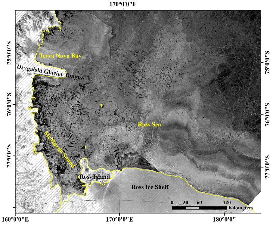
There are three polynyas in the Ross Sea: RISP, MSP, and TNBP, and their locations are shown in Figure 1. RISP is located along the Ross Ice Shelf, between Ross Island to the west and the 180° meridian to the east. MSP is located in the McMurdo Sound to the west of Ross Island. TNBP is located north of the Drygalski Glacier Tongue. In this study, we focus on the ice production of RISP and MSP.
2.2. Sentinel-1 Data
Sentinel-1 is the first of the Copernicus program satellite constellation conducted by the European space agency (ESA). It provides continuous all-weather, day-and-night radar imagery at the C-band. This mission is composed of a constellation of two satellites, Sentinel-1A and Sentinel-1B. Sentinel-1A was launched on 3 April 2014, and Sentinel-1B on 25 April 2016. They share the same orbital plane, with a repeat cycle of 12 days. Thus, after 25 April 2016, the combined repeat cycle is approximately 6 days, with almost daily revisit in the polar regions. These SAR instruments may acquire data in four exclusive modes: stripmap (SM), interferometric wide swath (IW), extra-wide swath (EW), and wave (WV). Among them, the modes EW and WV mainly operate over the ocean. For every mode, there are three kinds of products: level-0, level-1, and level-2. Level-0 is the SAR raw data. Level-1 products form a baseline product from which level-2 products are derived and consist of two types: SLC (single look complex) and GRD (ground range detected).
In this study, the level-1 GRD products of EW are used to detect coastal polynyas in the Ross Sea near the Ross Ice Shelf. The EW mode is used because of its wide swath (400 km) which results in larger areal coverage than the other modes. The spatial resolution of EW images is 25 m along-track by 100 m cross track.
The EW GRD SAR data are available in the ESA Open Access Hub (https://scihub.copernicus.eu/dhus/#/home). ESA provides software for processing Sentinel data called SNAP. In this study, the SNAP is used to process the EW GRD level-1 data, including radiometric calibration, speckle filtering, geometric ellipsoid correction, conversion to decibel value (dB), and mosaic data (if multiple images in one day). Radiometric calibration is used to convert the original number to the backscatter coefficient. The module “single product speckle filter” in SNAP is used to remove speckle noises in images with the Lee Sigma filter at a target window size of 3 × 3. The final projection of dB images is set to the stereographic South Pole, with a central meridian of 169°W and a standard parallel of −75°S, and a grid size of 40 m × 40 m.
All the sentinel-1 EW GRD data covering the RISP and MSP for the periods of 1 March–30 November 2017 and 2018 are downloaded and processed as explained above. Finally, a total of 143 images (days) in 2017 and 215 images (days) in 2018 are obtained to analyze the polynya ice production of these two periods.
2.3. AMSR2 Brightness Temperature
The advanced microwave scanning radiometer on JAXA’s GCOM-W1 (AMSR2), launched on 18 May 2012, scanned the earth twice per day (ascending and descending orbits). AMSR2 is a multi-frequency dual-polarized sensor and provides brightness temperatures in seven frequencies (6.93 GHz, 7.3 GHz, 10.65 GHz, 18.7 GHz, 23.8 GHz, 36.5 GHz, and 89.0 GHz) at both horizontal and vertical polarizations. The footprints of the data vary with frequency, the higher frequency with finer spatial resolution. In this study, the brightness temperatures at 36.5 GHz and 89.0 GHz for both polarizations in 2017 and 2018 are used to derive ice thickness in the Ross Sea based on the method in [19]. These brightness temperatures are retrieved from the “AMSR-E/AMSR2 Unified L3 Daily 12.5 km Brightness Temperatures, Sea Ice Concentration, Motion & Snow Depth Polar Grids V001” [49], archived in NASA (https://search.earthdata.nasa.gov/search). In this dataset, the brightness temperatures with different footprints are resampled to a grid size of 12 km × 12 km.
3. Method
The polynya ice productions in 2017 and 2018 are derived from Sentinel-1 SAR images and AMSR2 brightness temperatures. The former is used to identify the polynya area/extent and the latter is used to estimate sea ice thickness in the polynyas.
3.1. Detection of Polynya Area/Extent
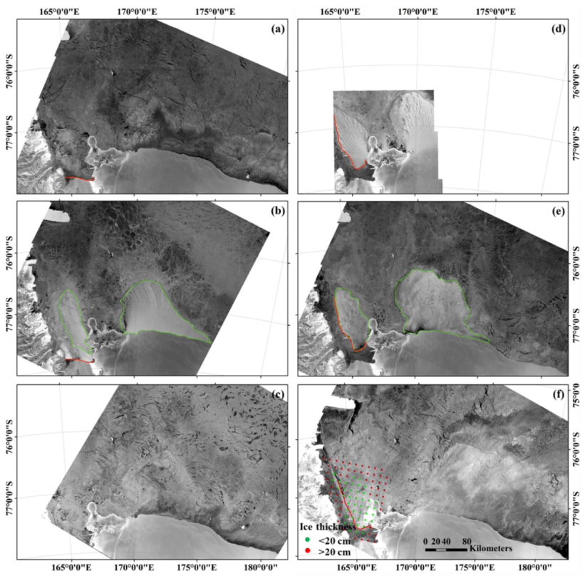
Polynyas in front of the Ross Ice Shelf and McMurdo Sound occur frequently due to the katabatic winds. Newly formed frazil and grease ice are self-organized into rows/strips approximately parallel to the wind direction (northward) and appear as white streaks that are early and visible in SAR imagery [41,42] as indicated in Figure 2 (green polygons as the mapped polynyas). The area characterized by white streaks (i.e., inside the green polygons) was called an “open polynya area” in some studies [41,50]. The open polynya area freezes quickly when the wind slows down, and the ice continues to grow (and thicken) until the next wind event that blows this newly formed ice away, ready for the subsequent new ice formation. So, the polynya ice production caused by such wind events is the ice volume blown away by the next wind event. The yearly polynya ice production is the total ice volume produced in the polynya by all wind events in the year. Noting that each ice production, although in the same general polynya area, would differ in production area/extent, shape, and thickness that are totally determined by the intensity, speed, and direction of each individual katabatic wind event and the length of the ice growth period before the next wind event. Figure 2 presents the evolution of such a large wind–driven ice production event, from no polynya (all covered by ice) on April 3 (Figure 2a), to a well–defined polynya with new ice formation on April 5 (Figure 2b), and to when the polynya ice completely merged with other ice on April 7 (Figure 2c). Polynyas in Figure 2b,e, although in the same general areas (MSP in the west and RSIP in the east), have different areas/extents, shapes, and thicknesses, due to different katabatic wind events (one on 5 April and the other on 19 August).
Although Sentinel-1 can scan the polar region daily, the study area is not always covered or fully covered, especially in 2017 when the study area was only scanned every other day; therefore, not all wind-driven polynya ice production events were imaged. Sometimes, the image only covers a portion of the study area. In these two cases, we try to determine the situation from the next available images with larger coverage, on which the outline/trace of the last polynya would be kept and mapped. For example, Figure 2e shows the same polynya not completely mapped/covered on 19 August (Figure 2d).
In the period of 17–21 September 2018 (Figure 3), three continuous ice formation/polynya events could be seen, marked with different color lines (red, green, and blue). The event 1 (red) was the first and biggest one and it is seen in all images (Figure 3a–d); the event 2 (green) started on 19 September (Figure 3b), and the event 3 (blue) started on 20 September (Figure 3c). On 21 September, the traces of all three ice formation events became obscure, except the event 1. Thus, even if one event was not captured due to no image collection at that time, it could be captured in a later image, based on the trace of the event. For example, in the wind-driven polynya event of 3–7 April 2017 (Figure 2a–c), the images were only available every other day. From the images on 5 April, only one wind-driven polynya can be seen. If any event occurred on 4 or 6 April, the event trace/outline could be seen on 5 or 7 April, just as seen from subsequent images in Figure 3. However, Figure 2 shows no additional event trace on the image of 5 April and no event trace on the image 7 April, meaning no event occurred on either 4 April or 6 April.
The extent/outline of every wind-driven polynya and ice formation event in 2017 and 2018 is visually observed and checked and then manually digitized according to the above-mentioned principle for identifying coastal polynya and the enclosed area, using ArcGIS software. Overall, we hope to express that the entire processing of identifying and mapping such an event trace/outline is not an easy task and it is tedious and time-consuming. This is currently the only way to assure the accuracy and confidence of our results.
Here we would like to demonstrate how we separate high backscatter values/appearances caused by wind-wave roughness from high backscatter values/appearances caused by wind-driven sea ice in polynyas, mainly from three aspects. (1) The texture of wind-wave caused high backscatter appearance differing from the texture of wind-driven sea ice. For example, the bright and homogeneous backscatter caused by wind-waves (Figure 4a) much differs from the wind–driven polynya sea ice (Figure 2b,d,e and Figure 3). (2) The sea ice concentration derived from the AMSR2 data shows the wind-wave event with very low ice concentration (<10%) (Figure 4b). (3) The shape of the wind-wave event does not exist after the wind event, differing from wind-driven polynya ice that keeps its shape until the next wind–driven event.
3.2. Retrieval of Ice Thickness
In this study, we use the AMSR2 brightness temperature at 89 and 36 GHz to derive thin ice thickness based on the algorithm in [19]. This algorithm was developed based on 186 MODIS ice thickness images and AMSR2 brightness temperatures in RISP, Ronne Ice Shelf Polynya, and Cape Darnley Polynya during April–September from 2013 to 2015. If the polarization ratio of 85 GHz (PR85) of a pixel is more than 0.062, the pixel is regarded as thin ice with thickness in the rage of 0–0.1 m, and the thickness H in meters is calculated using Equation (1). If the polarization ratio of 36 GHz (PR36) of a pixel is larger than 0.084, the pixel is regarded as thin ice with thicknesses ranging 0.1–0.2 m, and the thickness H in meters is calculated using Equation (2).
where TB85V and TB85H are the microwave brightness temperatures at 85 GHz for vertical and horizontal polarizations, respectively. TB36V and TB36H are the microwave brightness temperatures at 36 GHz for vertical and horizontal polarizations, respectively. For H < 10 cm, the root–mean–square error (RMSE) of the derived ice thickness is 5.6 cm, and the biases range from 0.8 to 3.8 cm; for 10 cm < H < 20 cm, the RMSE is 5.8 cm, and the biases range from −3.6 to 1.6 cm [19]. For cases when the computed thickness is less than 0 m, the thickness is assumed to be 0.01 m.
According to [19], the PMW method was only used for the derivation of ice thickness within 20 cm. Therefore, when ice thickness is larger than 20 cm based on Equations (1) and (2), the ice thickness is assumed to be 30 cm which is the average value of the observed ice thickness of more than 20 cm from the ship-based (ASPeCt) ice observations of PIPERS 2017 cruise during May/June 2017 in the RISP [51].
3.3. Calculation of Ice Volume
The ice volume is obtained by multiplying the ice area (from Sentinel-1) by the average thickness (from AMSR-2) in the ice area for each event. The cumulative ice volume is the sum of all ice production events within a year, normally between March and November.
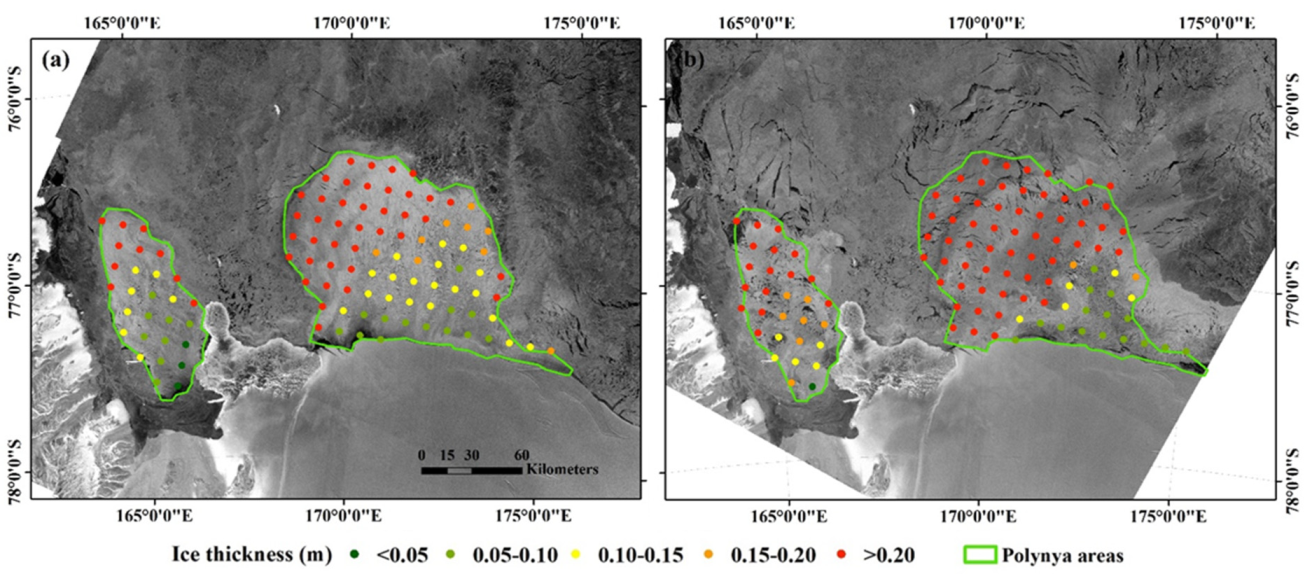
In this study, the ice thickness on the day prior to a next katabatic wind event is used for the calculation of ice production caused by this wind event. The reason is that the newly formed ice in a polynya would continuously grow until the next wind event blows away this ice to prepare for the next round of new ice production. Taking the data on 20 August 2017 as an example, in these two polynyas, ice thickness was inhomogeneous, and the average ice thicknesses in RISP and MSP were 0.20 m and 0.15 m (Figure 5a), respectively. The ice thicknesses in these two polynyas grew with time, and they reached at 0.26 m (at RISP) and 0.22 m (at MSP) on 22 August 2017 before the next wind event (Figure 5b). This polynya ice survived there 3 days before it was pushed away by the next wind-event for another new ice production.
4. Results
The extent/outline of each wind-driven polynya was manually digitized and the ice volume of each event was calculated based on the polynya area and ice thickness. The results are presented in Figure 6 and Table 2. During these two years of 2017 and 2018, the wind-driven polynya events occurred during March–November with no ice–production events observed during austral summertime (December, January, or February). The occurrence frequency of wind-driven polynya events was 90 in 2017, lower than 114 in 2018. Among them, there were 64 RISP events and 26 MSP events in 2017 (events occurred between 15 March and 15 November 2017), and 84 RISP and 30 MSP events in 2018 (events occurred from 12 March to 12 November 2018).
The polynya area and the ice production show large fluctuations (Figure 6). The areas of wind-driven polynya for each event varied from 343 km2 to 86,419 km2 for RISP, and from 159 km2 to 23,654 km2 for MSP. The yearly cumulative ice area in MSP was 93,327 km2 in 2017 and 87,682 km2 in 2018, and that of RISP were 1,066,520 km2 and 1,013,906 km2 (Figure 6, Table 2), respectively. The yearly cumulative ice productions were 14 km3 and 17 km3 for MSP in 2017 and 2018, and 188 km3 and 179 km3 for RISP in 2017 and 2018, respectively. Thus, it can be seen, although the occurrence frequency in 2017 was smaller than that in 2018, the yearly cumulative polynya areas and ice productions in 2017 were close to (even slightly larger than) those in 2018.
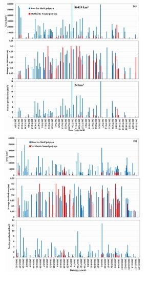
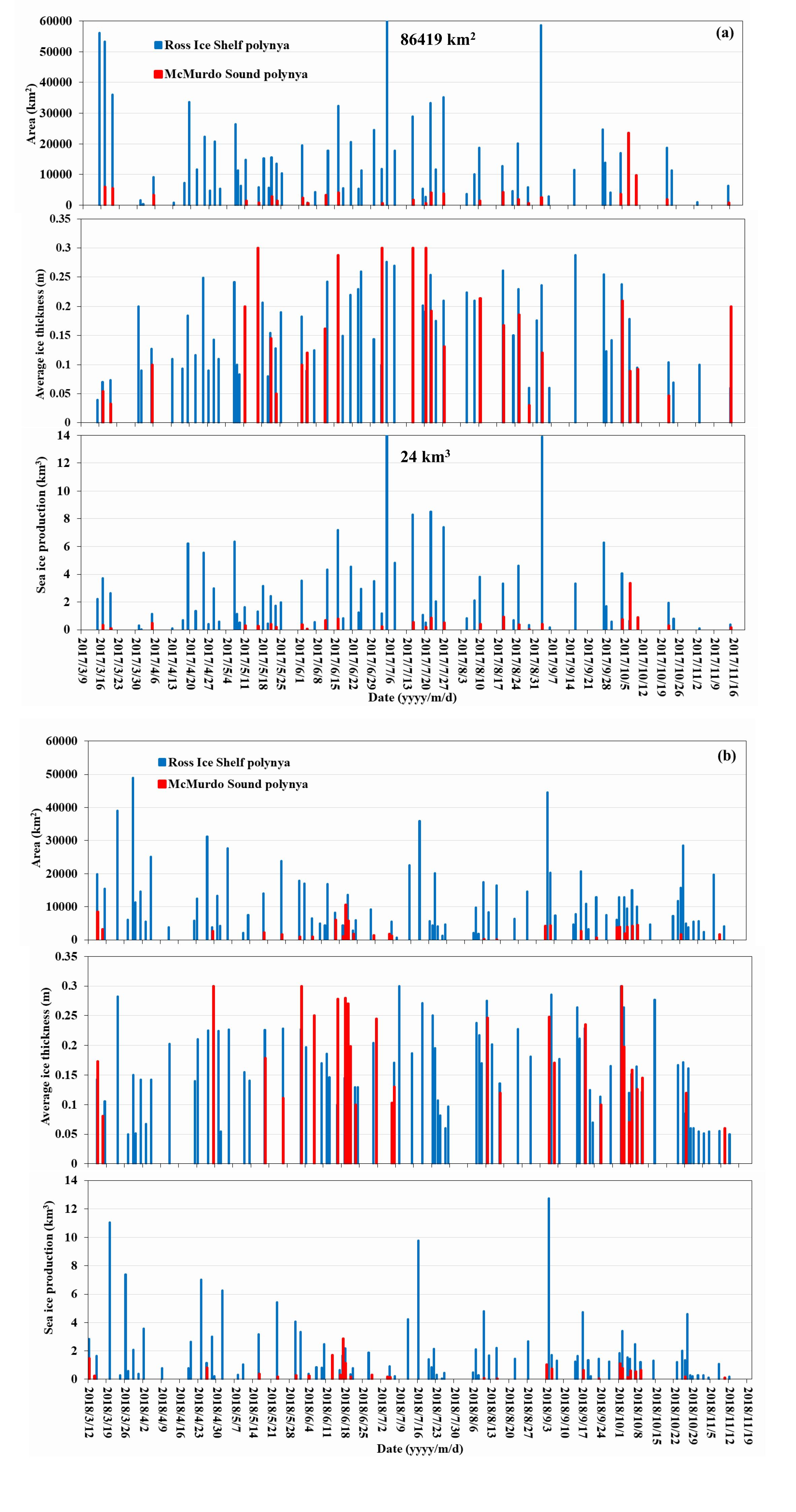
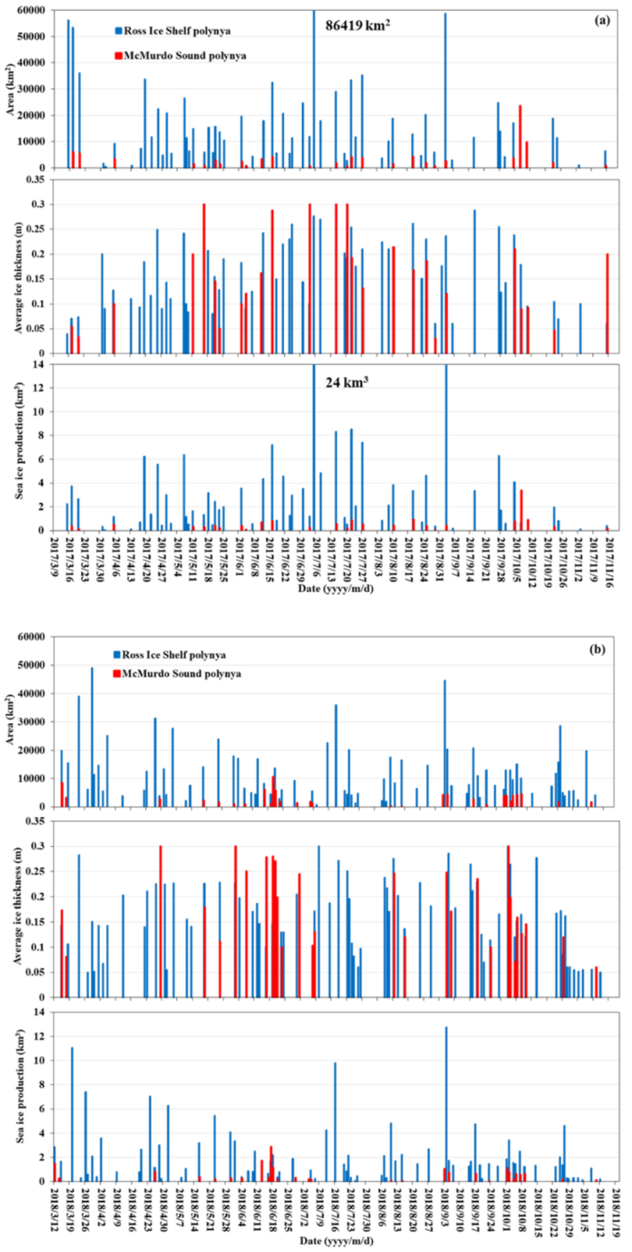
The cumulative polynya area is the area sum of all polynya events, and thus its value depends on occurrence frequency and each polynya area. Figure 6 shows the occurrence frequency in 2017 was smaller than that in 2018, but the frequency of polynya with an area of more than 3000 km2 was 9 in 2017, larger than 5 in 2018. Therefore, the average polynya area was 19,749 km2 (16,159 km2 for RISP and 3590 km2 for MSP) in 2017, much larger than 14,993 km2 (12,070 km2 for RSP and 2923 km2 for MSP) in 2018. Compared with the results in the previous studies, the polynya ice production in RSP is 1/2–2/3 of previous results, implying that previous studies might have significantly overestimated the ice production in RSP.
The cumulative polynya ice production is controlled by both polynya area/extent and ice thickness. The variability in average ice thicknesses of RISP and MSP in 2017 and 2018 (Figure 6) shows that during 2017, the minimum ice thicknesses of all ice production events at the RISP and MSP are 0.05 m and 0.03 m, respectively; the maximum ice thicknesses are 0.29 m and 0.3 m, respectively; and the average thicknesses are 0.18 m and 0.16 m, respectively. During 2018, the minimum ice thicknesses of all ice-production events in RISP and MSP were 0.05 m and 0.06 m, respectively; the maximum ice thicknesses are 0.30 m and 0.30 m, respectively; and the average thicknesses were 0.16 m and 0.18 m, respectively. Although ice thickness was quite variable over time, there was an apparent seasonal change of increase-stable-decrease, i.e., increase from March to May, relatively stable from May to September, and decrease from September onwards.
In some days when Katabatic winds occurred continuously, such as in the periods of 17–22 June 2018 and 21–26 July 2018, the ice thicknesses were approximately 0.1–0.13 m, thinner than that of other times in the stable phase (Figure 5), because there was not enough time for sea ice to grow. So, the high–frequency of occurrence is one of the reasons for thin ice thickness, which also influences the ice production of each polynya event.
In previous studies presented in Table 1, the polynya area was defined as the area with an ice thickness of less than 20 cm or the ice concentration of less than 75% from March to October [19,23,39], hereafter referred as the PMW method. The ice thickness and concentration were estimated from PMW based on PR36 and PR85 [23,49]. In this study, the same PMW method is also used to estimate the average polynya area (March to October) in 2017 and 2018 based on AMSR2, and the results show that the annual average areas of RISP and MSP were 23,617 km2 and 1782 km2 in 2017, respectively, and 25,901 km2 and 1874 km2 in 2018, respectively (Table 2). The estimated polynya areas from PWM are much larger than the polynya areas from Sentinel-1 SAR in RSIP but much lower in MSP.
5. Discussion
The polynya area and polynya ice production estimated in this study are different from those in previous studies. The reasons for this difference are analyzed in this section. The method to derive wind-driven polynya and ice production is different from the PMW method. For the PMW method, thin ice thickness (<20 cm) was first estimated from PMW based on PR36 and PR85 or the ice concentration less than 75%, and then the sea ice production was calculated by the heat flux model based on the thin ice thickness data from March to October [23]. Therefore, it was not possible to identify individual polynya events, (i.e., neither it was possible to compute individual event area or volume). Previous studies in Table 1 present the average polynya area, which was the mean thin ice area of all days from March to October. This mean ice area was then used to generate ice production volume based on the heat flux calculation. Furthermore, in the PMW method, the difference in the definition of polynya (based on ice thickness or ice concentration) might directly influence the ice production results, therefore, papers showed different results even for the same year [19,39].
In this study, Sentinel-1 SAR data is used to obtain the individual wind–driven polynya ice production events and their corresponding areas, with very fine spatial and temporal resolutions. For example, from the SAR images, the wind-driven polynyas occurred 2 times in November 2017 and 5 times in November 2018, while in the PMW method, the ice production was only accounted for the period of March–October. In terms of ice thickness for the ice volume calculation in this study, the last ice thickness from the PMW in the day before the next wind-driven event is used. The PMW method, however, cannot determine such information for individual ice production events.
Furthermore, in previous studies, the polynya area was thought of as the thin ice area, and the ice production had a very high correlation with the polynya area (0.89) [21]. However, it can be seen from Sentinel-l SAR data (e.g., Figure 6) that some areas exhibit an ice thickness of more than 20 cm within the polynyas, while the PMW method would not count as ice production. This could result in underestimates of ice production. On the other hand, the fast ice area was very likely misclassified as the polynya area by PMW method, due to the potential underestimation in fast ice thickness (Figure 2f). This uncertainty was pointed out by [52] in which they developed a new fast-ice mask method to improve the sea ice production calculation from AMSR–E.
Compared with previous studies performed based on PMW and heat flux model, the results of this study show much lower ice production estimates in the RISP. It is worth noting that the PMW method usually has large uncertainties in estimating the polynya area. The annual ice production in the RISP and MSP vary from 160 km3 to 600 km3 (Table 1). Even for similar time periods, different papers obtained different results like in [25] and [8]. The former paper calculated the ice production from 1992 to 2002, and the latter one from 1992 to 2001. The difference in average annual ice production between the two studies was more than 100 km3. In addition, using different data sources or different definitions of polynya areas in the PMW method may also result in differences in estimates. For example, based on [19], the ice productions from AMSR-E/2, with finer resolution, were smaller than that from SSM/I, with coarser resolution. The ice production in the same year from [39] that used ice concentration to determine the polynya area, and from [19] that applied ice thickness to determine the polynya area were different.
The annual average areas of RISP and MSP in 2017 and 2018 estimated from the PMW are consistent with previous studies. However, these numbers are much different from what is mapped from Sentinel-1 in this paper (Table 2). For example, in the RISP, the polynya areas from AMSR2 are much larger than those from our method, but in the MSP, the polynya areas from AMSR2 is only half of the value from our method in these two years. This is mostly due to different definitions of the polynya area between the PMW method and our method. However, due to the limited image data in 2017 and the short time period (only 2 years of data) examined, it is still difficult to determine if this difference in the two years is significant or not. Our next step is to extend this study further to 2019, 2020, and beyond.
Although SAR can be used to accurately detect polynya because of its high spatial resolution, some uncertainties in ice production estimation in this study remain to be further examined. The polynya areas in the current study are derived by manually digitizing the outline/trace of the polynya-covered ice area, based on visual observations and experiences. This is time-consuming and labor-intensive. Due to the manually digitizing, the data sets are not easy to be reproduced or automatically extracted. Automated methods have been developed to identify the polynya area based on COSMO-SkyMed X-SAR and ERS C-SAR data [40,41,53,54], and the results showed high agreement with manual results. However, these methods have not yet been used to derive time series of polynya areas, and are not applied in the condition that the polynya extent/outline in the gap days obtained, totally based on visual observation and experiences, from the images after the gap days. In future work, the automatic method is hoped to be developed based on the Sentinel-1 SAR, to estimate time series of polynya areas, using machine learning/deep learning methods. The ice thickness algorithm was developed for the thin ice area (ice thickness less than 20 cm), and the estimation accuracy would decrease when the ice thickness is larger than 20 cm. In this study, we see the ice thickness could be larger than 20 cm in the polynya area and we assume such thickness to be 30 cm, based on the average value of the observed ice thickness of more than 20 cm from the PIPERS 2017 cruise (ASPeCt ice observations) over the RISP, in May/June 2017. This assumption would cause some uncertainties. Satellite–based altimetry is a promising method to derive accurate sea ice thickness [46,47]. The launch of ICESat-2 provides a great opportunity to estimate freeboard/ice thickness starting in September 2018; therefore, it is our next step to use ICESat-2 to derive ice thickness for ice production estimation.
6. Conclusions
In this study, the high spatial and temporal resolution of Sentinel–1 SAR data are used to derive the wind–driven ice production of Ross Sea polynyas in 2017 and 2018.
Based on the Sentinels SAR imagery, the wind-driven polynyas occurred from the middle of March to the middle of November. There were 90 wind-driven polynya events in 2017 (64 in RISP and 26 in MSP) and 114 events in 2018 (84 in RISP and 30 in MSP), the yearly cumulative polynya area were 1,159,847 km2 in 2017 and 1,101,588 km2 in 2018, and the yearly cumulative polynya ice productions were 202 km3 in 2017 and 196 km3 in 2018. The polynya event frequency in 2017 was less than that in 2018, but the yearly cumulative polynya area and ice production were similar to those in 2018. The more frequent events mean the shorter time for ice growth in polynya, then the smaller ice thickness.
The yearly cumulative SIP volume is only 1/2–2/3 of those reported from previous results. The reason for this difference may come from the different methods and the uncertainties of each method. In the method of this study, every polynya event was derived using manually digitization based on the SAR images, and the events occurred from the middle of March to the middle of November. This is different from the definition in the PMW method in which the polynya area was the mean daily area with an ice thickness of less than 20 cm for the period of March to October. The ice volume in this study was calculated through multiplying the polynya area and the ice thickness estimated from AMSR2. For the PMW method, the ice production was estimated by the heat flux model. The estimation algorithm of ice thickness and the inputs of the heat flux model could also bring in uncertainties in the ice production estimation. The results in this study imply that the previous studies might have significantly overestimated the ice production in the RSP. However, due to the limited image data in 2017 and the short time (only 2 years) of data, some uncertainties still exist. We hope the longer time series of ice productions will be obtained in the future to further assess this method.
Author Contributions
Methodology, L.D., H.X.; Supervision, H.X., S.F.A.; Writing–original draft, L.D.; Writing–review & editing, H.X., S.F.A. and A.M.M.-N. All authors have read and agreed to the published version of the manuscript.
Funding
L. Dai was supported by the Strategic Priority Research Program of the Chinese Academy of Sciences (no. XDA19070101) and the National Natural Science Foundation of China (no. 41771389). Supports for H. Xie, S. Ackley, and A. Mestas were provided by the U.S. National Science Foundation (no. 134717 and 1835784) and U.S. National Aeronautics and Space Administration (NASA) (no. 80NSSC19M0194).
Acknowledgments
L. Dai thanks the China Scholarship Council for funding her 2016–2017 visit to the University of Texas at San Antonio. The European Space Agency (ESA) provided Sentinel–1 SAR data, NASA provided AMSR2 brightness temperature and sea ice concentration data. Critical reviews from three anonymous reviewers to substantially improve the paper are greatly appreciated.
Conflicts of Interest
The authors declare no conflict of interest.
References
- Bromwich, D.H.; Kurtz, D.D. Katabatic wind forcing of the Terra Nova Bay polynya. J. Geophys. Res. 1984, 89, 3561. [Google Scholar] [CrossRef]
- Bromwich, D.; Liu, Z.; Rogers, A.N.; Van Woert, M.L. Winter atmospheric forcing of the Ross Sea polynya. Ocean ICE Atmos. Int. Antarct. Cont. Margin 1998, 75, 101–133. [Google Scholar]
- Bromwich, D.H.; Carrasco, J.F.; Liu, Z.; Tzeng, R.Y. Hemispheric atmospheric variations and oceanographic impacts associated with katabatic surges across the ross ice shelf, Antarctica. J. Geophys. Res.–Atmos. 1993, 98, 13045–13062. [Google Scholar] [CrossRef]
- Sansiviero, M.; Maqueda, M.A.M.; Fusco, G.; Aulicino, G.; Flocco, D.; Budillon, G. Modelling sea ice formation in the Terra Nova Bay polynya. J. Mar. Syst. 2017, 166, 4–25. [Google Scholar] [CrossRef]
- Fusco, G.; Budillon, G.; Spezie, G. Surface heat fluxes and thermohaline variability in the Ross Sea and in Terra Nova Bay polynya. Cont. Shelf Res. 2009, 29, 1887–1895. [Google Scholar] [CrossRef]
- Kusahara, K.; Hasumi, H.; Tamura, T. Modeling sea ice production and dense shelf water formation in coastal polynyas around East Antarctica. J. Geophys. Res.–Oceans 2010, 115, C10006. [Google Scholar] [CrossRef] [Green Version]
- Wilkinson, J.P.; Wadhams, P. A salt flux model for salinity change through ice production in the Greenland Sea, and its relationship to winter convection. J. Geophys. Res. 2003, 108, 3147. [Google Scholar] [CrossRef]
- Tamura, T.; Ohshima, K.I.; Nihashi, S. Mapping of sea ice production for Antarctic coastal polynyas. Geophys. Res. Lett. 2008, 35, L07606. [Google Scholar] [CrossRef]
- Kimura, N.; Wakatsuchi, M. Increase and decrease of sea ice area in the Sea of Okhotsk: Ice production in coastal polynyas and dynamic thickening in convergence zones. J. Geophys. Res.–Oceans 2004, 109, C09S03. [Google Scholar] [CrossRef] [Green Version]
- Assmann, K.M.; Hellmer, H.H.; Jacobs, S.S. Amundsen Sea ice production and transport. J. Geophys. Res. 2005, 110, C12013. [Google Scholar] [CrossRef] [Green Version]
- Tamura, T.; Williams, G.D.; Fraser, A.D.; Ohshima, K.I. Potential regime shift in decreased sea ice production after the Mertz Glacier calving. Nat. Commun. 2012, 3, 826. [Google Scholar] [CrossRef] [PubMed] [Green Version]
- Ohshima, K.I.; Fukamachi, Y.; Williams, G.D.; Nihashi, S.; Roquet, F.; Kitade, Y.; Tamura, T.; Hirano, D.; Herraiz-Borreguero, L.; Field, I.; et al. Antarctic Bottom Water production by intense sea–ice formation in the Cape Darnley polynya. Nat. Geosci. 2013, 6, 235–240. [Google Scholar] [CrossRef]
- Orsi, A.H.; Johnson, G.C.; Bullister, J.L. Circulation, mixing, and production of Antarctic Bottom Water. Prog. Oceanogr. 1999, 43, 55–109. [Google Scholar] [CrossRef]
- Kitade, Y.; Shimada, K.; Tamura, T.; Williams, G.D.; Aoki, S.; Fukamachi, Y.; Ohshima, K.I. Antarctic Bottom Water production from the Vincennes Bay Polynya, East Antarctica. Geophys. Res. Lett. 2014, 41, 3528–3534. [Google Scholar] [CrossRef] [Green Version]
- Krumpen, T.; Holemann, J.A.; Willmes, S.; Maqueda, M.A.M.; Busche, T.; Dmitrenko, I.A.; Schroder, D. Sea ice production and water mass modification in the eastern Laptev Sea. J. Geophys. Res.–Oceans 2011, 116, C05014. [Google Scholar] [CrossRef] [Green Version]
- Ito, M.; Ohshima, K.I.; Fukamachi, Y.; Mizuta, G.; Kusumoto, Y.; Nishioka, J. Observations of frazil ice formation and upward sediment transport in the Sea of Okhotsk: A possible mechanism of iron supply to sea ice. J. Geophys. Res.–Oceans 2017, 122, 788–802. [Google Scholar] [CrossRef]
- Grossmann, S.; Dieckmann, G.S. Bacterial Standing Stock, Activity, and Carbon Production during Formation and Growth of Sea–Ice in the Weddell Sea, Antarctica. Appl. Environ. Microb. 1994, 60, 2746–2753. [Google Scholar] [CrossRef] [Green Version]
- Nihashi, S.; Ohshima, K.I.; Saitoh, S.I. Sea–ice production in the northern Japan Sea. Deep–Sea Res. Part I 2017, 127, 65–76. [Google Scholar] [CrossRef]
- Nihashi, S.; Ohshima, K.I.; Tamura, T. Sea–Ice Production in Antarctic Coastal Polynyas Estimated From AMSR2 Data and Its Validation Using AMSR–E and SSM/I–SSMIS Data. IEEE J.–Stars 2017, 10, 3912–3922. [Google Scholar] [CrossRef] [Green Version]
- Hollands, T.; Dierking, W. Dynamics of the Terra Nova Bay Polynya: The potential of multi–sensor satellite observations. Remote Sens. Environ. 2016, 187, 30–48. [Google Scholar] [CrossRef] [Green Version]
- Tamura, T.; Ohshima, K.I.; Fraser, A.D.; Williams, G.D. Sea ice production variability in Antarctic coastal polynyas. J. Geophys. Res.–Oceans 2016, 121, 2967–2979. [Google Scholar] [CrossRef] [Green Version]
- Kashiwase, H.; Ohshima, K.I.; Nihashi, S. Long–term variation in sea ice production and its relation to the intermediate water in the Sea of Okhotsk. Prog. Oceanogr. 2014, 126, 21–32. [Google Scholar] [CrossRef]
- Tamura, T.; Ohshima, K.I. Mapping of sea ice production in the Arctic coastal polynyas. J. Geophys. Res. 2011, 116, C07030. [Google Scholar] [CrossRef]
- Drucker, R.; Martin, S.; Kwok, R. Sea ice production and export from coastal polynyas in the Weddell and Ross Seas. Geophys. Res. Lett. 2011, 38, L1705. [Google Scholar] [CrossRef] [Green Version]
- Martin, S.; Drucker, R.S.; Kwok, R. The areas and ice production of the western and central Ross Sea polynyas, 1992–2002, and their relation to the B–15 and C–19 iceberg events of 2000 and 2002. J. Mar. Syst. 2007, 68, 201–214. [Google Scholar] [CrossRef]
- Parmiggiani, F. Multi–year measurement of Terra Nova Bay winter polynya extents. Eur. Phys. J. Plus 2011, 126. [Google Scholar] [CrossRef]
- Toggweiler, J.R.; Samuels, B. Effect of Sea–Ice on the Salinity of Antarctic Bottom Waters. J. Phys. Oceanogr. 1995, 25, 1980–1997. [Google Scholar] [CrossRef] [Green Version]
- Goosse, H.; Campin, J.M.; Fichefet, T.; Deleersnijder, E. Impact of sea–ice formation on the properties of Antarctic bottom water. Ann. Glaciol. 1997, 25, 276–281. [Google Scholar] [CrossRef] [Green Version]
- Ciappa, A.; Pietranera, L.; Budillon, G. Observations of the Terra Nova Bay (Antarctica) polynya by MODIS ice surface temperature imagery from 2005 to 2010. Remote Sens. Environ. 2012, 119, 158–172. [Google Scholar] [CrossRef]
- Aulicino, G.; Sansiviero, M.; Paul, S.; Cesarano, C.; Fusco, G.; Wadhams, P.; Budillon, G. A New Approach for Monitoring the Terra Nova Bay Polynya through MODIS Ice Surface Temperature Imagery and Its Validation during 2010 and 2011 Winter Seasons. Remote Sens. 2018, 10, 366. [Google Scholar] [CrossRef] [Green Version]
- Paul, S.; Willmes, S.; Heinemann, G. Long–term coastal–polynya dynamics in the southern Weddell Sea from MODIS thermal–infrared imagery. Cryosphere 2015, 9, 2027–2041. [Google Scholar] [CrossRef] [Green Version]
- Preusser, A.; Heinemann, G.; Willmes, S.; Paul, S. Circumpolar polynya regions and ice production in the Arctic: Results from MODIS thermal infrared imagery from 2002/2003 to 2014/2015 with a regional focus on the Laptev Sea. Cryosphere 2016, 10, 3021–3042. [Google Scholar] [CrossRef] [Green Version]
- Paul, S.; Willmes, S.; Gutjahr, O.; Preußer, A.; Heinemann, G. Spatial Feature Reconstruction of Cloud–Covered Areas in Daily MODIS Composites. Remote Sens. 2015, 7, 5042–5056. [Google Scholar] [CrossRef] [Green Version]
- Willmes, S.; Heinemann, G. Pan–Arctic lead detection from MODIS thermal infrared imagery. Ann. Glaciol. 2015, 56, 29–37. [Google Scholar] [CrossRef] [Green Version]
- Ludwig, V.; Spreen, G.; Haas, C.; Istomina, L.; Kauker, F.; Murashkin, D. The 2018 North Greenland polynya observed by a newly introduced merged optical and passive microwave sea– ice concentration dataset. Cryosphere 2019, 13, 2051–2073. [Google Scholar] [CrossRef] [Green Version]
- Zwally, H.J.; Comiso, J.C.; Gordon, A.L. Antarctic offshore leads and polynyas and oceanographic effects. In Oceanology of the Antarctic Continental Shelf; Jacobs, S.S., Ed.; American Geophysical Union: Washington, DC, USA, 1985; Volume 43, pp. 203–226. [Google Scholar] [CrossRef] [Green Version]
- Arrigo, K.R.; van Dijken, G.L. Phytoplankton dynamics within 37 Antarctic coastal polynya systems. J. Geophys. Res.–Oceans 2003, 108, 3271. [Google Scholar] [CrossRef]
- Comiso, J.C.; Kwok, R.; Martin, S.; Gordon, A.L. Variability and trends in sea ice extent and ice production in the Ross Sea. J. Geophys. Res.–Oceans 2011, 116, C04021. [Google Scholar] [CrossRef] [Green Version]
- Cheng, Z.; Pang, X.P.; Zhao, X.; Stein, A. Heat Flux Sources Analysis to the Ross Ice Shelf Polynya Ice Production Time Series and the Impact of Wind Forcing. Remote Sens. 2019, 11, 188. [Google Scholar] [CrossRef] [Green Version]
- Dokken, S.T.; Winsor, P.; Markus, T.; Askne, J.; Bjork, G. ERS SAR characterization of coastal polynyas in the Arctic and comparison with SSM/I and numerical model investigations. Remote Sens. Environ. 2002, 80, 321–335. [Google Scholar] [CrossRef]
- Ciappa, A.; Pietranera, L. High resolution observations of the Terra Nova Bay polynya using COSMO–SkyMed X–SAR and other satellite imagery. J. Mar. Syst. 2013, 113, 42–51. [Google Scholar] [CrossRef]
- Kwok, R.; Comiso, J.C.; Martin, S.; Drucker, R. Ross Sea polynyas: Response of ice concentration retrievals to large areas of thin ice. J. Geophys. Res.–Oceans 2007, 112, C12012. [Google Scholar] [CrossRef] [Green Version]
- Parmiggiani, F. Fluctuations of Terra Nova Bay polynya as observed by active (ASAR) and passive (AMSR–E) microwave radiometers. Int. J. Remote Sens. 2006, 27, 2459–2467. [Google Scholar] [CrossRef]
- Laxon, S.W.; Giles, K.A.; Ridout, A.L.; Wingham, D.J.; Willatt, R.; Cullen, R.; Davidson, M. CryoSat–2 estimates of Arctic sea ice thickness and volume. Geophys. Res. Lett. 2013, 40, 732–737. [Google Scholar] [CrossRef] [Green Version]
- Li, H.; Xie, H.J.; Kern, S.; Wan, W.; Ozsoy, B.; Ackley, S.; Hong, Y. Spatio–temporal variability of Antarctic sea–ice thickness and volume obtained from ICESat data using an innovative algorithm. Remote Sens. Environ. 2018, 219, 44–61. [Google Scholar] [CrossRef]
- Price, D.; Rack, W.; Langhorne, P.J.; Haas, C.; Leonard, G.; Barnsdale, K. The sub–ice platelet layer and its influence on freeboard to thickness conversion of Antarctic sea ice. Cryosphere 2014, 8, 1031–1039. [Google Scholar] [CrossRef] [Green Version]
- Rack, W.; Haas, C.; Langhorne, P.J. Airborne thickness and freeboard measurements over the McMurdo Ice Shelf, Antarctica, and implications for ice density. J. Geophys. Res.–Oceans 2013, 118, 5899–5907. [Google Scholar] [CrossRef]
- Xia, W.T.; Xie, H.J. Assessing three waveform retrackers on sea ice freeboard retrieval from Cryosat–2 using Operation IceBridge Airborne altimetry datasets. Remote Sens. Environ. 2018, 204, 456–471. [Google Scholar] [CrossRef]
- Meier, W.N.; Markus, T.; Comiso, J.C. AMSR–E/AMSR2 Unified L3 Daily 12.5 km Brightness Temperatures, Sea Ice Concentration, Motion & Snow Depth Polar Grids, Version 1. [ Brightness temperatures at 36 GHz and 85 GHz from 1 January 2017 to 31 March 2019]. Boulder, Colorado USA. NASA National Snow and Ice Data Center Distributed Active Archive Center. 2018. Available online: https://nsidc.org/data/au_si12/versions/1 (accessed on 5 August 2019).
- Drucker, R.; Martin, S.; Moritz, R. Observations of ice thickness and frazil ice in the St. Lawrence Island polynya from satellite imagery, upward looking sonar, and salinity/temperature moorings. J. Geophys. Res.–Oceans 2003, 108, 3149. [Google Scholar] [CrossRef]
- Ackley, S.F.; Stammerjohn, S.; Maksym, T.; Smith, M.; Cassano, J.; Guest, P.; Tison, J.-L.; Delille, B.; Loose, B.; Sedwick, P.; et al. Sea ice production and air-ocean-ice-biogeochemistry interactions in the Ross Sea during the PIPERS 2017 autumn field campaign. Ann. Glaciol. 2020. [Google Scholar] [CrossRef]
- Iwamoto, K.; Ohshima, K.I.; Tamura, T. Improved mapping of sea ice production in the Arctic Ocean using AMSR–E thin ice thickness algorithm. J. Geophys. Res.–Oceans 2014, 119, 3574–3594. [Google Scholar] [CrossRef]
- Galley, R.J.; Barber, D.G.; Yackel, J.J. On the link between SAR–derived sea ice melt and development of the summer upper ocean mixed layer in the North Open Water Polynya. Int. J. Remote Sens. 2007, 28, 3979–3994. [Google Scholar] [CrossRef]
- Flores, M.M.; Parmiggiani, F.; Lopez, L.L. Automatic Measurement of Polynya Area by Anisotropic Filtering and Markov Random Fields. IEEE J.–Stars 2014, 7, 1665–1674. [Google Scholar] [CrossRef]
Figure 1.
Sentinel-1 SAR image of the Ross Sea with the coastal boundary and named locations of the Ross Ice Shelf, Ross Island, Drygalski Glacier Tongue, McMurdo Sound, Terra Nova Bay, and the Ross Sea.
Figure 1.
Sentinel-1 SAR image of the Ross Sea with the coastal boundary and named locations of the Ross Ice Shelf, Ross Island, Drygalski Glacier Tongue, McMurdo Sound, Terra Nova Bay, and the Ross Sea.

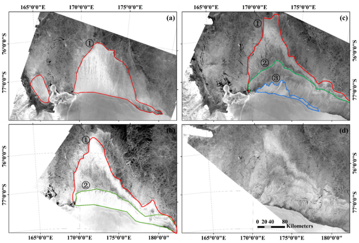
Figure 2.
Examples of Sentinel-1 SAR images on 3 April 2017 (a) (no polynya), 5 April 2017 (b) (clear polynya), and 7 April 2017 (c) (disappearance of polynya); 19 August 2017 (d) and 20 August 2017 (e) together explain the incomplete scan in (d); 28 October 2018 (f) indicating the thin ice (green dots) from passive microwave data overlaying the Sentinel-1 SAR image in the McMurdo Sound. The green (red) dots indicate ice thicknesses <20 cm (>20 cm) and the solid red line is the McMurdo fast ice edge.

Figure 3.
Sentinel-1 images in the Ross Sea on 17 September (a), 19(b), 20(c), 21(d) in 2018. During these days, three katabatic wind events occurred. The first one occurred on 17 September (with the polynya area sketched as the red line ①) and finished on 19 September. The second event occurred on 19 September (with the polynya area sketched as the green line ②) and finished on 20 September. The third event occurred on 20 September (sketched as the blue line ③) and calmed down on 21 September when all traces, except the first one, are more diffuse.

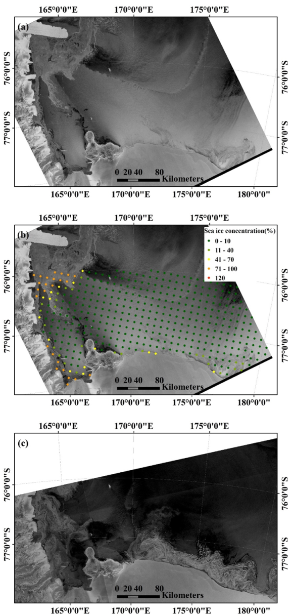
Figure 4.
Sentinel-1 images (backscatter) of Ross Sea on 3–4 March 2017: (a) backscatter image on 3 March showing bright and homogeneous wind-driven roughness, (b) less than 10% ice concentration (from AMSR2) on the bright and homogeneous wind-driven roughness (3 March), and (c) disappearance of wind-driven roughness after the wind event on 4 March.

Figure 5.
Polynya area (green polygons) mapped from the Sentinel-1 SAR image on 20 August 2017, and the ice thicknesses (dots) within the polynya area derived from AMSR2 on 20 August 2017 (a) and 22 August 2017 (b).
Figure 5.
Polynya area (green polygons) mapped from the Sentinel-1 SAR image on 20 August 2017, and the ice thicknesses (dots) within the polynya area derived from AMSR2 on 20 August 2017 (a) and 22 August 2017 (b).

Figure 6.
Wind-driven ice production areas, average thickness, and volumes for every event at the McMurdo Sound and Ross Ice Shelf polynyas (RISP) in 2017 (a) and 2018 (b). (The polynya area and polynya ice production of RISP on July 5, 2017, exceed the top scale. They are 86,419 km2, and 24 km3, respectively).


Table 1.
Statistics of polynya ice production in the Ross Sea presented in previous studies.
| Temporal Periods | Mean Daily Area (km2) | Mean Annual Cumulative Volume (km3) | Data Sources | References |
|---|---|---|---|---|
| 1987 | RISP + MSP = 25,000 | SMMR | Zwally et al. (1985) [36] | |
| 1992–2002 | RISP = 25,000 ± 5000 MSP = 2000 ± 600 | RISP = 500 ± 160 | SSM/I | Martin et al. (2007) [25] |
| 1992–2001 | RISP + MSP = 390 ± 59 | SSM/I | Tamura et al. (2008) [8] | |
| 1997–2002 | RISP + MSP = 20,000 | SSM/I | Arrigo and Van Dijken (2003) [37] | |
| 1992–2008 | RISP + MSP + TNBP = 930,000 | RISP = 602 MSP = 47 | SSM/I | Drucker et al. (2011) [24] |
| 1992–2013 | RISP + MSP = 22,000 ± 3000 | RISP + MSP = 382 ± 63 | SSM/I | Tamura et al. (2016) [21] |
| 2000–2008 | RISP + MSP = 30,000 | RISP + MSP = 600 | SSM/I | Comiso et al. (2011) [38] |
| 1992–1999 | RISP + MSP = 350 | SSM/I | ||
| 2003–2011 | RISP + MSP = 300 ± 20 RISP + MSP = 316 ± 34 | AMSR–E SSM/I | Nihashi et al. (2017b) [19] | |
| 2013–2015 | RISP + MSP = 317 ± 18 RISP + MSP = 340 ± 32 | AMSR2 SSMI/S | Nihashi et al. (2017b) [19] | |
| 2003–2017 | RISP = 164~313 | AMSR–E AMSR2 | Cheng et al. (2019) [39] |
Table 2.
Statistics of wind–driven polynya ice production events in the Ross Ice Shelf polynya (RISP) and McMurdo Sound polynya (MSP) during 2017 and 2018. The mean ice production event areas derived from AMSR-2 (ice thickness < 20 cm) are also included for comparison.
Table 2.
Statistics of wind–driven polynya ice production events in the Ross Ice Shelf polynya (RISP) and McMurdo Sound polynya (MSP) during 2017 and 2018. The mean ice production event areas derived from AMSR-2 (ice thickness < 20 cm) are also included for comparison.
| Year | 2017 | 2018 | ||
|---|---|---|---|---|
| Polynyas | RISP | MSP | RISP | MSP |
| Event times | 64 | 26 | 84 | 30 |
| Cumulative area (km2) | 1,066,520 | 93,327 | 1,013,906 | 87,682 |
| Mean event area (km2) | 16,159 | 3590 | 12,070 | 2923 |
| Cumulative Volume (km3) | 188 | 14 | 179 | 17 |
| Mean daily area from AMSR2 (km2) | 23,617 | 1782 | 25,901 | 1874 |
© 2020 by the authors. Licensee MDPI, Basel, Switzerland. This article is an open access article distributed under the terms and conditions of the Creative Commons Attribution (CC BY) license (http://creativecommons.org/licenses/by/4.0/).
Share and Cite
MDPI and ACS Style
Dai, L.; Xie, H.; Ackley, S.F.; Mestas-Nuñez, A.M. Ice Production in Ross Ice Shelf Polynyas during 2017–2018 from Sentinel–1 SAR Images. Remote Sens. 2020, 12, 1484. https://0-doi-org.brum.beds.ac.uk/10.3390/rs12091484
AMA Style
Dai L, Xie H, Ackley SF, Mestas-Nuñez AM. Ice Production in Ross Ice Shelf Polynyas during 2017–2018 from Sentinel–1 SAR Images. Remote Sensing. 2020; 12(9):1484. https://0-doi-org.brum.beds.ac.uk/10.3390/rs12091484
Chicago/Turabian StyleDai, Liyun, Hongjie Xie, Stephen F. Ackley, and Alberto M. Mestas-Nuñez. 2020. "Ice Production in Ross Ice Shelf Polynyas during 2017–2018 from Sentinel–1 SAR Images" Remote Sensing 12, no. 9: 1484. https://0-doi-org.brum.beds.ac.uk/10.3390/rs12091484
Note that from the first issue of 2016, this journal uses article numbers instead of page numbers. See further details here.