Identifying Post-Fire Recovery Trajectories and Driving Factors Using Landsat Time Series in Fire-Prone Mediterranean Pine Forests


Abstract
:
1. Introduction
2. Materials and Methods
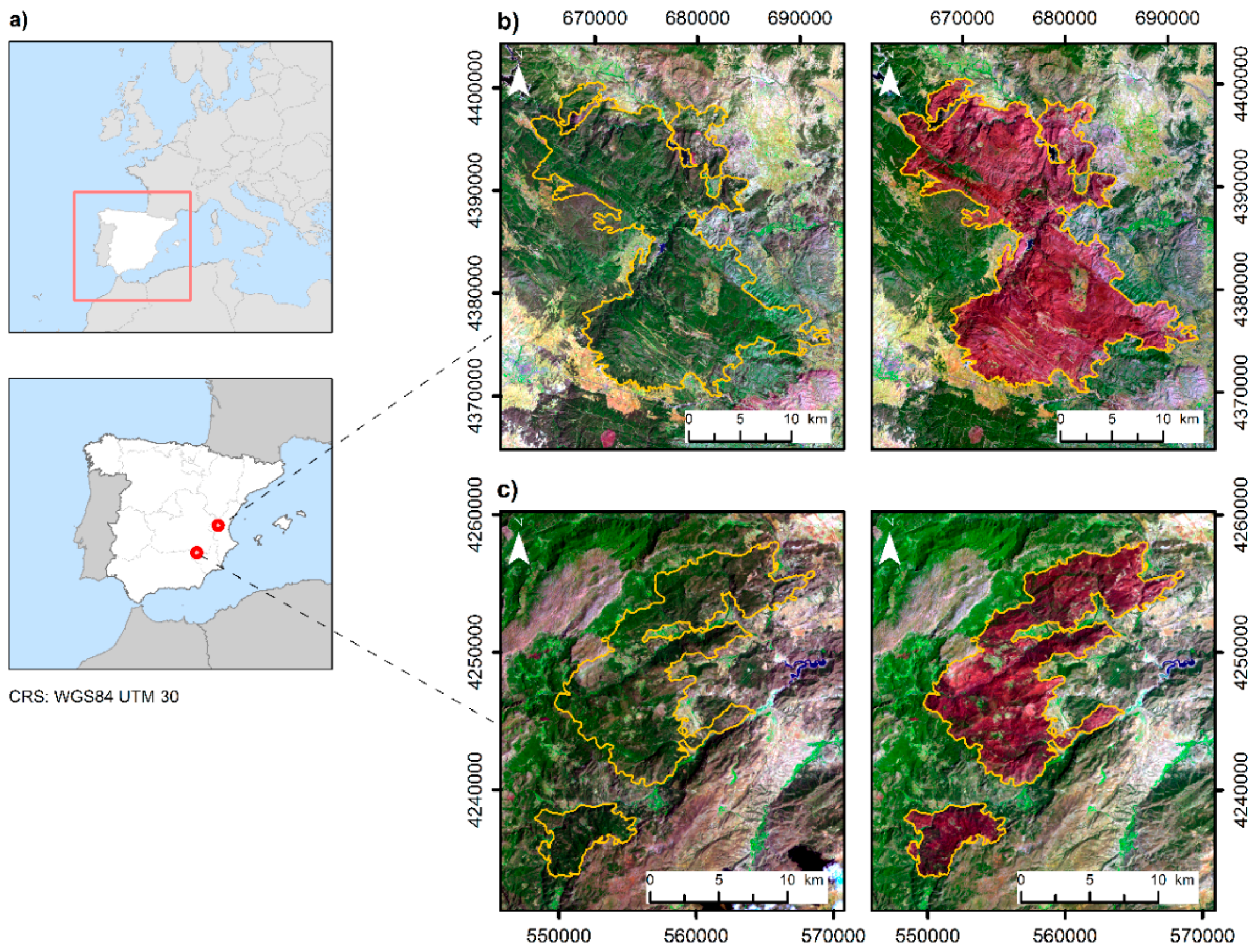
2.1. Study Area
2.2. Data
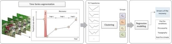
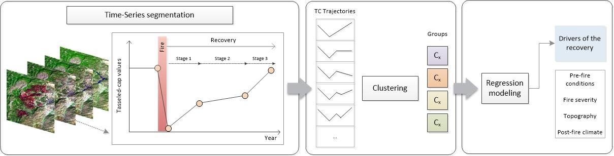
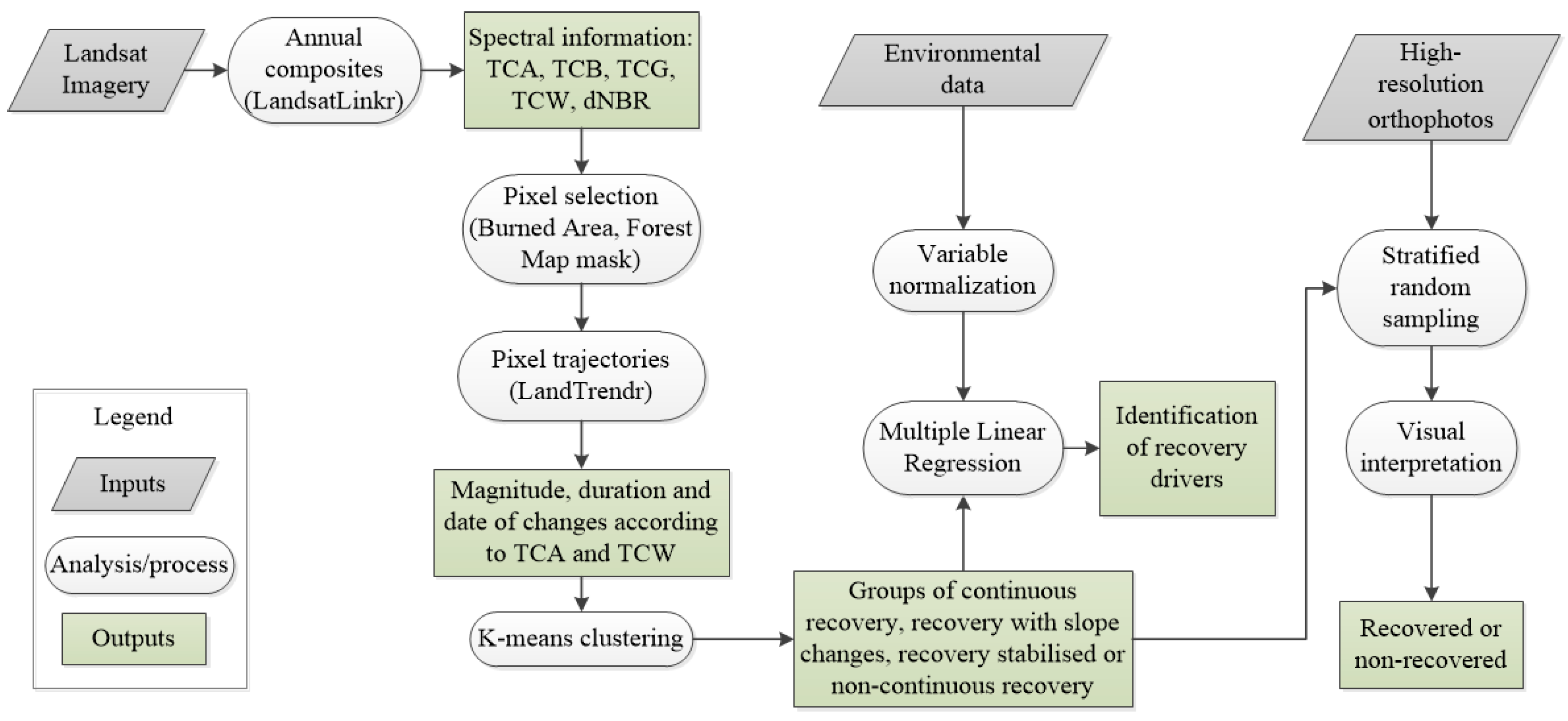
2.3. Methods
2.3.1. Landsat Time Series
2.3.2. Trajectory Segmentation and Clustering
2.3.3. Assessing Driving Factors of Vegetation Recovery
2.3.4. Recovery Assessment
3. Results
3.1. Classification of Post-Fire Trajectories
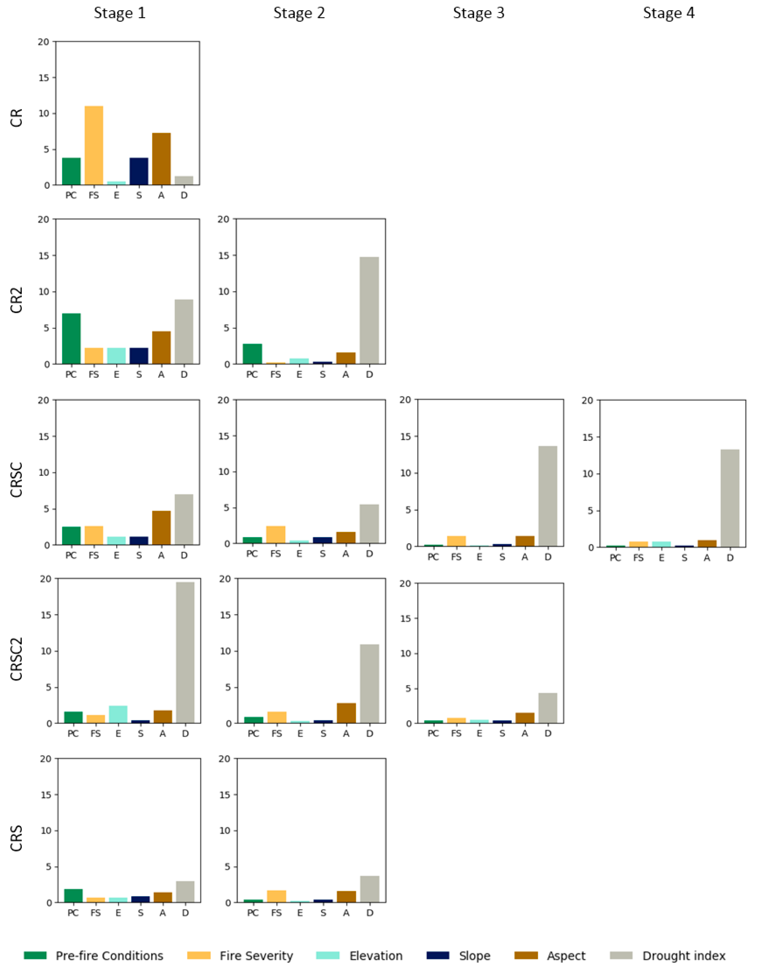
3.2. Assessing Drivers of Post-Fire Vegetation Recovery
3.3. Recovery Estimation Assessment
4. Discussion
4.1. Post-Fire Recovery Trajectories from LTS
Accuracy Assessment of Post-Fire Recovery
4.2. Assessment of Post-Fire Recovery Drivers
5. Conclusions
Author Contributions
Funding
Conflicts of Interest
References
- Bowman, D.M.J.S.; Balch, J.K.; Artaxo, P.; Bond, W.J.; Carlson, J.M.; Cochrane, M.A.; D’Antonio, C.M.; DeFries, R.S.; Doyle, J.C.; Harrison, S.P.; et al. Fire in the earth system. Science 2009, 324, 481–484. [Google Scholar] [CrossRef] [PubMed]
- Chuvieco, E. Global impacts of fire. In Earth Observation of Wildland Fires in Mediterranean Ecosystems; Chuvieco, E., Ed.; Springer: Berlin, Germany, 2009; pp. 1–10. ISBN 9783642017537. [Google Scholar]
- Aponte, C.; de Groot, W.J.; Wotton, M. Forest fires and climate change: Causes, consequences and management options. Int. J. Wildl. Fire 2016, 25, 861–875. [Google Scholar] [CrossRef]
- San-Miguel-Ayanz, J.; Durrant, T.; Boca, R.; Liberta`, G.; Branco, A.; De Rigo, D.; Ferrari, D.; Maianti, P.; Artes Vivancos, T.; Pfeiffer, H.; et al. Forest Fires in Europe, Middle East and North Africa 2018; Publications Office of the European Union: Luxembourg, 2019; ISBN 9789279928321. [Google Scholar]
- San-Miguel-Ayanz, J.; Moreno, J.M.; Camia, A. Analysis of large fires in European Mediterranean landscapes: Lessons learned and perspectives. For. Ecol. Manag. 2013, 294, 11–22. [Google Scholar] [CrossRef]
- Keeley, J.E.; Bond, W.J.; Bradstock, R.A.; Pausas, J.G.; Rundel, P.W. Fire in Mediterranean Ecosystems: Ecology, Evolution and Management; Cambridge University Press: Cambridge, UK, 2014; Volume 10, ISBN 9780521824910. [Google Scholar]
- De las Heras, J.; Moya, D.; Vega, J.A.; Daskalakou, E.; Vallejo, R.; Grigoriadis, N.; Tsitsoni, T.; Baeza, J.; Valdecantos, A.; Fernández, C.; et al. Post-fire management of serotinous pine forests. In Post-Fire Management and Restoration of Southern European Forests; Moreira, F., Arianoutsou, M., Corona, P., de las Heras, J., Eds.; Springer: Berlin, Germany, 2012; Volume 24, pp. 121–149. ISBN 978-94-007-2207-1. [Google Scholar]
- González-De Vega, S.; de las Heras, J.; Moya, D. Post-fire regeneration and diversity response to burn severity in Pinus halepensis Mill. Forests. Forests 2018, 9, 299. [Google Scholar] [CrossRef] [Green Version]
- Pausas, J.G.; Keeley, J.E. A burning story: The role of fire in the history of life. Bioscience 2009, 59, 593–601. [Google Scholar] [CrossRef] [Green Version]
- Stephens, S.L.; Agee, J.K.; Fulé, P.Z.; North, M.P.; Romme, W.H.; Swetnam, T.W.; Turner, M.G. Managing forests and fire in changing climates. Science 2013, 342, 41–42. [Google Scholar] [CrossRef]
- Lindner, M.; Maroschek, M.; Netherer, S.; Kremer, A.; Barbati, A.; Garcia-Gonzalo, J.; Seidl, R.; Delzon, S.; Corona, P.; Kolström, M.; et al. Climate change impacts, adaptive capacity, and vulnerability of European forest ecosystems. For. Ecol. Manag. 2010, 259, 698–709. [Google Scholar] [CrossRef]
- González-De Vega, S.; De las Heras, J.; Moya, D. Resilience of Mediterranean terrestrial ecosystems and fire severity in semiarid areas: Responses of Aleppo pine forests in the short, mid and long term. Sci. Total Environ. 2016, 573, 1171–1177. [Google Scholar] [CrossRef]
- Gitas, I.; Mitri, G.; Veraverbeke, S.; Polychronaki, A. Advances in remote sensing of post-fire vegetation recovery monitoring—A review. In Remote Sensing of Biomass—Principles and Applications; IntechOpen: London, UK, 2012. [Google Scholar]
- Banskota, A.; Kayastha, N.; Falkowski, M.J.; Wulder, M.A.; Froese, R.E.; White, J.C. Forest monitoring using Landsat time series data: A review. Can. J. Remote Sens. 2014, 40, 362–384. [Google Scholar] [CrossRef]
- Wulder, M.A.; Loveland, T.R.; Roy, D.P.; Crawford, C.J.; Masek, J.G.; Woodcock, C.E.; Allen, R.G.; Anderson, M.C.; Belward, A.S.; Cohen, W.B.; et al. Current status of Landsat program, science, and applications. Remote Sens. Environ. 2019, 225, 127–147. [Google Scholar] [CrossRef]
- Meng, R.; Dennison, P.E.; Huang, C.; Moritz, M.A.; D’Antonio, C. Effects of fire severity and post-fire climate on short-term vegetation recovery of mixed-conifer and red fir forests in the Sierra Nevada Mountains of California. Remote Sens. Environ. 2015, 171, 311–325. [Google Scholar] [CrossRef]
- Fernandez-Manso, A.; Quintano, C.; Roberts, D.A. Burn severity influence on post-fire vegetation cover resilience from Landsat MESMA fraction images time series in Mediterranean forest ecosystems. Remote Sens. Environ. 2016, 184, 112–123. [Google Scholar] [CrossRef]
- Ireland, G.; Petropoulos, G.P. Exploring the relationships between post-fire vegetation regeneration dynamics, topography and burn severity: A case study from the Montane Cordillera Ecozones of Western Canada. Appl. Geogr. 2015, 56, 232–248. [Google Scholar] [CrossRef]
- Pickell, P.D.; Hermosilla, T.; Frazier, R.J.; Coops, N.C.; Wulder, M.A. Forest recovery trends derived from Landsat time series for North American boreal forests. Int. J. Remote Sens. 2016, 37, 138–149. [Google Scholar] [CrossRef]
- Chu, T.; Guo, X.; Takeda, K. Effects of burn severity and environmental conditions on post-fire regeneration in Siberian Larch forest. Forests 2017, 8, 76. [Google Scholar] [CrossRef]
- Shvetsov, E.G.; Kukavskaya, E.A.; Buryak, L.V.; Barrett, K. Assessment of post-fire vegetation recovery in Southern Siberia using remote sensing observations. Environ. Res. Lett. 2019, 14, 055001. [Google Scholar] [CrossRef]
- Griffiths, P.; Kuemmerle, T.; Baumann, M.; Radeloff, V.C.; Abrudan, I.V.; Lieskovsky, J.; Munteanu, C.; Ostapowicz, K.; Hostert, P. Forest disturbances, forest recovery, and changes in forest types across the carpathian ecoregion from 1985 to 2010 based on landsat image composites. Remote Sens. Environ. 2014, 151, 72–88. [Google Scholar] [CrossRef]
- DeVries, B.; Decuyper, M.; Verbesselt, J.; Zeileis, A.; Herold, M.; Joseph, S. Tracking disturbance-regrowth dynamics in tropical forests using structural change detection and Landsat time series. Remote Sens. Environ. 2015, 169, 320–334. [Google Scholar] [CrossRef]
- Lhermitte, S.; Verbesselt, J.; Verstraeten, W.W.; Veraverbeke, S.; Coppin, P. Assessing intra-annual vegetation regrowth after fire using the pixel based regeneration index. ISPRS J. Photogramm. Remote Sens. 2011, 66, 17–27. [Google Scholar] [CrossRef] [Green Version]
- Kennedy, R.E.; Yang, Z.; Cohen, W.B.; Pfaff, E.; Braaten, J.; Nelson, P. Spatial and temporal patterns of forest disturbance and regrowth within the area of the Northwest Forest Plan. Remote Sens. Environ. 2012, 122, 117–133. [Google Scholar] [CrossRef]
- White, J.C.; Wulder, M.A.; Hermosilla, T.; Coops, N.C.; Hobart, G.W. A nationwide annual characterization of 25 years of forest disturbance and recovery for Canada using Landsat time series. Remote Sens. Environ. 2017, 194, 303–321. [Google Scholar] [CrossRef]
- Frazier, R.J.; .Coops, N.C.; Wulder, M.A.; Hermosilla, T.; White, J.C. Analyzing spatial and temporal variability in short-term rates of post-fire vegetation return from Landsat time series. Remote Sens. Environ. 2018, 205, 32–45. [Google Scholar] [CrossRef]
- Bright, B.C.; Hudak, A.T.; Kennedy, R.E.; Braaten, J.D.; Henareh Khalyani, A. Examining post-fire vegetation recovery with Landsat time series analysis in three western North American forest types. Fire Ecol. 2019, 15, 8. [Google Scholar] [CrossRef] [Green Version]
- Zhu, Z. Change detection using landsat time series: A review of frequencies, preprocessing, algorithms, and applications. ISPRS J. Photogramm. Remote Sens. 2017, 130, 370–384. [Google Scholar] [CrossRef]
- Röder, A.; Hill, J.; Duguy, B.; Alloza, J.A.; Vallejo, R. Using long time series of Landsat data to monitor fire events and post-fire dynamics and identify driving factors. A case study in the Ayora region (eastern Spain). Remote Sens. Environ. 2008, 112, 259–273. [Google Scholar] [CrossRef]
- Hope, A.; Tague, C.; Clark, R. Characterizing post-fire vegetation recovery of California chaparral using TM/ETM+ time-series data. Int. J. Remote Sens. 2007, 28, 1339–1354. [Google Scholar] [CrossRef]
- Kennedy, R.E.; Yang, Z.G.; Cohen, W.B. Detecting trends in forest disturbance and recovery using yearly Landsat time series: 1. LandTrendr—Temporal segmentation algorithms. Remote Sens. Environ. 2010, 114, 2897–2910. [Google Scholar] [CrossRef]
- Huang, C.; Goward, S.N.; Masek, J.G.; Thomas, N.; Zhu, Z.; Vogelmann, J.E. An automated approach for reconstructing recent forest disturbance history using dense Landsat time series stacks. Remote Sens. Environ. 2010, 114, 183–198. [Google Scholar] [CrossRef]
- Verbesselt, J.; Hyndman, R.; Newnham, G.; Culvenor, D. Detecting trend and seasonal changes in satellite image time series. Remote Sens. Environ. 2010, 114, 106–115. [Google Scholar] [CrossRef]
- Zhu, Z.; Woodcock, C.E.; Olofsson, P. Continuous monitoring of forest disturbance using all available Landsat imagery. Remote Sens. Environ. 2012, 122, 75–91. [Google Scholar] [CrossRef]
- Nguyen, T.H.; Jones, S.D.; Soto-Berelov, M.; Haywood, A.; Hislop, S. A spatial and temporal analysis of forest dynamics using Landsat time-series. Remote Sens. Environ. 2018, 217, 461–475. [Google Scholar] [CrossRef]
- Viana-Soto, A.; Aguado, I.; Martínez, S. Assessment of Post-Fire Vegetation Recovery Using Fire Severity and Geographical Data in the Mediterranean Region (Spain). Environments 2017, 4, 90. [Google Scholar] [CrossRef] [Green Version]
- Hislop, S.; Jones, S.; Soto-Berelov, M.; Skidmore, A.; Haywood, A.; Nguyen, T.H. Using Landsat spectral indices in time-series to assess wildfire disturbance and recovery. Remote Sens. 2018, 10, 460. [Google Scholar] [CrossRef] [Green Version]
- Key, C.H.; Benson, N.C. Landscape assessment: Remote sensing of severity, the Normalized Burn Ratio. In FIREMON: Fire Effects Monitoring and Inventory System; USDA Forest Service, Rocky Mountain Research Station, Fort Collins: Denver, CO, USA, 2006; pp. 305–325. [Google Scholar]
- Morresi, D.; Vitali, A.; Urbinati, C.; Garbarino, M. Forest spectral recovery and regeneration dynamics in stand-replacing wildfires of central Apennines derived from Landsat time series. Remote Sens. 2019, 11, 308. [Google Scholar] [CrossRef] [Green Version]
- Crist, E.P. A TM Tasseled Cap equivalent transformation for reflectance factor data. Remote Sens. Environ. 1985, 17, 301–306. [Google Scholar] [CrossRef]
- Gómez, C.; White, J.C.; Wulder, M.A. Characterizing the state and processes of change in a dynamic forest environment using hierarchical spatio-temporal segmentation. Remote Sens. Environ. 2011, 115, 1665–1679. [Google Scholar] [CrossRef]
- Pflugmacher, D.; Cohen, W.B.; Kennedy, R.E.; Yang, Z. Using Landsat-derived disturbance and recovery history and lidar to map forest biomass dynamics. Remote Sens. Environ. 2014, 151, 124–137. [Google Scholar] [CrossRef]
- Frazier, R.J.; Coops, N.C.; Wulder, M.A. Boreal Shield forest disturbance and recovery trends using Landsat time series. Remote Sens. Environ. 2015, 170, 317–327. [Google Scholar] [CrossRef]
- Hansen, M.J.; Franklin, S.E.; Woudsma, C.; Peterson, M. Forest structure classification in the North Columbia mountains using the Landsat TM Tasseled Cap wetness component. Can. J. Remote Sens. 2001, 27, 20–32. [Google Scholar] [CrossRef]
- Powell, S.L.; Cohen, W.B.; Healey, S.P.; Kennedy, R.E.; Moisen, G.G.; Pierce, K.B.; Ohmann, J.L. Quantification of live aboveground forest biomass dynamics with Landsat time-series and field inventory data: A comparison of empirical modeling approaches. Remote Sens. Environ. 2010, 114, 1053–1068. [Google Scholar] [CrossRef]
- Gómez, C.; Wulder, M.A.; White, J.C.; Montes, F.; Delgado, J.A. Characterizing 25 years of change in the area, distribution, and carbon stock of Mediterranean pines in Central Spain. Int. J. Remote Sens. 2012, 33, 5546–5573. [Google Scholar] [CrossRef]
- Martín-Alcón, S.; Coll, L. Unraveling the relative importance of factors driving post-fire regeneration trajectories in non-serotinous Pinus nigra forests. For. Ecol. Manag. 2016, 361, 13–22. [Google Scholar] [CrossRef] [Green Version]
- Oliver, C.; Larson, B. Forest Stand Dynamics (Update Edition); Wiley: New York, NY, USA, 1996; Volume 42. [Google Scholar]
- Bartels, S.F.; Chen, H.Y.H.; Wulder, M.A.; White, J.C. Trends in post-disturbance recovery rates of Canada’s forests following wildfire and harvest. For. Ecol. Manag. 2016, 361, 194–207. [Google Scholar] [CrossRef] [Green Version]
- Rivas-Martínez, S. Etages bioclimatiques, secteurs chorologiques et séries de végétation de l’Espagne méditerranéenne. An. del Jardín Botánico Madr. 1981, 37, 251–268. [Google Scholar]
- Ministerio de Agricultura Pesca y Alimentación. Second National Forest Inventory of Spain. Available online: https://www.miteco.gob.es/es/biodiversidad/servicios/banco-datos-naturaleza/informacion-disponible/ifn2.aspx (accessed on 27 January 2020).
- Fernández-García, V.; Fulé, P.Z.; Marcos, E.; Calvo, L. The role of fire frequency and severity on the regeneration of Mediterranean serotinous pines under different environmental conditions. For. Ecol. Manag. 2019, 444, 59–68. [Google Scholar] [CrossRef]
- Eugenio, M.; Verkaik, I.; Lloret, F.; Espelta, J.M. Recruitment and growth decline in Pinus halepensis populations after recurrent wildfires in Catalonia (NE Iberian Peninsula). For. Ecol. Manag. 2006, 231, 47–54. [Google Scholar]
- Moya, D.; González-De Vega, S.; García-Orenes, F.; Morugán-Coronado, A.; Arcenegui, V.; Mataix-Solera, J.; Lucas-Borja, M.E.; De las Heras, J. Temporal characterisation of soil-plant natural recovery related to fire severity in burned Pinus halepensis Mill. forests. Sci. Total Environ. 2018, 640–641, 42–51. [Google Scholar] [CrossRef]
- Crotteau, J.S.; Morgan Varner, J.; Ritchie, M.W. Post-fire regeneration across a fire severity gradient in the southern Cascades. For. Ecol. Manag. 2013, 287, 103–112. [Google Scholar] [CrossRef]
- United States Geological Survey (USGS). Earth Explorer Server. Available online: https://earthexplorer.usgs.gov/ (accessed on 27 January 2020).
- Masek, J.G.; Vermote, E.F.; Saleous, N.E.; Wolfe, R.; Hall, F.G.; Huemmrich, K.F.; Gao, F.; Kutler, J.; Lim, T.-K. A Landsat surface reflectance dataset for North America, 1990–2000. IEEE Geosci. Remote Sens. Lett. 2006, 3, 68–72. [Google Scholar] [CrossRef]
- Vermote, E.; Justice, C.; Claverie, M.; Franch, B. Preliminary analysis of the performance of the Landsat 8/OLI land surface reflectance product. Remote Sens. Environ. 2016, 185, 46–56. [Google Scholar] [CrossRef]
- Miller, J.D.; Thode, A.E. Quantifying burn severity in a heterogeneous landscape with a relative version of the delta Normalized Burn Ratio (dNBR). Remote Sens. Environ. 2007, 109, 66–80. [Google Scholar] [CrossRef]
- Ministerio de Agricultura Pesca y Alimentación. Forest Map of Spain. Available online: https://www.miteco.gob.es/es/biodiversidad/servicios/banco-datos-naturaleza/informacion-disponible/mfe200.aspx (accessed on 27 January 2020).
- Spain National Geographic Institute (IGN). Digital Elevation Model 25-m. Available online: http://centrodedescargas.cnig.es/CentroDescargas/index.jsp (accessed on 7 February 2020).
- Vicente-Serrano, S.M.; Tomas-Burguera, M.; Beguería, S.; Reig, F.; Latorre, B.; Peña-Gallardo, M.; Luna, M.Y.; Morata, A.; González-Hidalgo, J.C. A high resolution dataset of drought indices for Spain. Data 2017, 2, 22. [Google Scholar] [CrossRef] [Green Version]
- Vicente-Serrano, S.M.; Beguería, S.; López-Moreno, J.I. A multiscalar drought index sensitive to global warming: The standardized precipitation evapotranspiration index. J. Clim. 2010, 23, 1696–1718. [Google Scholar] [CrossRef] [Green Version]
- Spain National Geographic Institute (IGN). Aerial Orthophotography National Plan. Available online: http://centrodedescargas.cnig.es/CentroDescargas/index.jsp (accessed on 7 February 2020).
- Braaten, J.D.; Cohen, W.B.; Yang, Z. LandsatLinkr. Zenodo. Available online: https://zenodo.org/record/1231029#.XrPS5MARWUk (accessed on 20 January 2020).
- Vogeler, J.C.; Braaten, J.D.; Slesak, R.A.; Falkowski, M.J. Extracting the full value of the Landsat archive: Inter-sensor harmonization for the mapping of Minnesota forest canopy cover (1973–2015). Remote Sens. Environ. 2018, 209, 363–374. [Google Scholar] [CrossRef]
- Hartigan, J.A.; Wong, M.A. Algorithm AS 136: A K-Means Clustering Algorithm. J. R. Stat. Soc. Ser. C Appl. Stat. 1979, 28, 100–108. [Google Scholar] [CrossRef]
- Gouveia, C.; DaCamara, C.C.; Trigo, R.M. Post-fire vegetation recovery in Portugal based on spot/vegetation data. Nat. Hazards Earth Syst. Sci. 2010, 10, 673–684. [Google Scholar] [CrossRef] [Green Version]
- Purnima, B.; Arvind, K. EBK-Means: A Clustering Technique based on Elbow Method and K-Means in WSN. Int. J. Comput. Appl. 2014, 105, 17–24. [Google Scholar]
- Varoquaux, G.; Buitinck, L.; Louppe, G.; Grisel, O.; Pedregosa, F.; Mueller, A. Scikit-learn. GetMobile Mob. Comput. Commun. 2015, 19, 29–33. [Google Scholar] [CrossRef]
- Roberts, D.W.; Cooper, S.V. Concepts and techniques of vegetation mapping. Pages 90–96 BT—Compilers. Land classifications based on vegetation: Applications for resource management. In USDA Forest Service General Technical Report INT-257; Ferguson, D.E., Morgan, P., Johnson, F.D., Eds.; Intermountain Research Station: Ogden, UT, USA, 1989. [Google Scholar]
- Lentile, L.B.; Holden, Z.A.; Smith, A.M.S.; Falkowski, M.J.; Hudak, A.T.; Morgan, P.; Lewis, S.A.; Gessler, P.E.; Benson, N.C. Remote sensing techniques to assess active fire characteristics and post-fire effects. Int. J. Wildl. Fire 2006, 15, 319–345. [Google Scholar] [CrossRef]
- Vicente-Serrano, S.M.; Gouveia, C.; Camarero, J.J.; Beguería, S.; Trigo, R.; López-Moreno, J.I.; Azorín-Molina, C.; Pasho, E.; Lorenzo-Lacruz, J.; Revuelto, J.; et al. Response of vegetation to drought time-scales across global land biomes. Proc. Natl. Acad. Sci. USA 2013, 110, 52–57. [Google Scholar] [CrossRef] [Green Version]
- Fotheringham, A.S.; Brunsdon, C.; Charlton, M. Geographically weighted regression: The analysis of spatially varying relationships; John Wiley & Sons: Hoboken, NJ, USA, 2003; ISBN 0-471-49616-2. [Google Scholar]
- Brunsdon, C.; Fotheringham, A.S.; Charlton, M.E. Geographically Weighted Regression: A Method for Exploring Spatial Nonstationarity. Geogr. Anal. 2010, 28, 281–298. [Google Scholar] [CrossRef]
- Hurvich, C.M.; Simonoff, J.S.; Tsai, C.-L. Smoothing parameter selection in nonparametric regression using an improved Akaike information criterion. J. R. Stat. Soc. Ser. B Stat. Methodol. 1998, 60, 271–293. [Google Scholar] [CrossRef]
- Zhao, F.R.; Meng, R.; Huang, C.; Zhao, M.; Zhao, F.A.; Gong, P.; Yu, L.; Zhu, Z. Long-term post-disturbance forest recovery in the greater yellowstone ecosystem analyzed using Landsat time series stack. Remote Sens. 2016, 8, 898. [Google Scholar] [CrossRef] [Green Version]
- Congalton, R.G.; Green, K. Assessing the Accuracy of Remotely Sensed Data: Principles and Practices; Lewis Publishers: Boca Raton, FL, USA, 1999; ISBN 0873719867. [Google Scholar]
- Schroeder, T.A.; Wulder, M.A.; Healey, S.P.; Moisen, G.G. Mapping wildfire and clearcut harvest disturbances in boreal forests with Landsat time series data. Remote Sens. Environ. 2011, 115, 1421–1433. [Google Scholar] [CrossRef]
- Thanos, C.A.; Daskalakou, E.N. Reproduction in Pinus halepensis and P. brutia. In Ecology, Biogeography and Management of Pinus Halepensis and P. Brutia Forest Ecosystems in the Mediterranean Basin; Backhuys Publishers: Leiden, The Netherlands, 2000; pp. 79–90. [Google Scholar]
- Viana Soto, A.; Aguado, I.; Salas, J.; García, M. Classification of post-fire recovery trajectories using Landsat time series in the Mediterranean region: Spain. In Earth Resources and Environmental Remote Sensing/GIS Applications; International Society for Optics and Photonics: Strasbourg, France, 2019; Volume 1115607, p. 6. [Google Scholar]
- Tanase, M.; de la Riva, J.; Santoro, M.; Pérez-Cabello, F.; Kasischke, E. Sensitivity of SAR data to post-fire forest regrowth in Mediterranean and boreal forests. Remote Sens. Environ. 2011, 115, 2075–2085. [Google Scholar] [CrossRef]
- Martín-Alcón, S.; Coll, L.; De Cáceres, M.; Guitart, L.; Cabré, M.; Just, A.; González-Olabarría, J.R. Combining aerial LiDAR and multispectral imagery to assess postfire regeneration types in a Mediterranean forest. Can. J. For. Res. 2015, 45, 856–866. [Google Scholar] [CrossRef]
- Bolton, D.K.; Coops, N.C.; Wulder, M.A. Characterizing residual structure and forest recovery following high-severity fire in the western boreal of Canada using Landsat time-series and airborne lidar data. Remote Sens. Environ. 2015, 163, 48–60. [Google Scholar] [CrossRef]
- Cohen, W.B.; Yang, Z.; Kennedy, R. Detecting trends in forest disturbance and recovery using yearly Landsat time series: 2. TimeSync—Tools for calibration and validation. Remote Sens. Environ. 2010, 114, 2911–2924. [Google Scholar] [CrossRef]
- Storey, E.A.; Stow, D.A.; Roberts, D.A. Evaluating uncertainty in Landsat-derived postfire recovery metrics due to terrain, soil, and shrub type variations in southern California. GIScience Remote Sens. 2020, 57, 352–368. [Google Scholar] [CrossRef]
- Liu, Z. Effects of climate and fire on short-term vegetation recovery in the boreal larch forests of northeastern China. Sci. Rep. 2016, 6, 37572. [Google Scholar] [CrossRef] [Green Version]
- Pausas, J.G.; Ouadah, N.; Ferran, A.; Gimeno, T.; Vallejo, R. Fire severity and seedling establishment in Pinus halepensis woodlands, eastern Iberian Peninsula. Plant Ecol. 2002, 169, 205–213. [Google Scholar] [CrossRef]
- Baudena, M.; Santana, V.M.; Baeza, M.J.; Bautista, S.; Eppinga, M.B.; Hemerik, L.; Garcia Mayor, A.; Rodriguez, F.; Valdecantos, A.; Vallejo, V.R.; et al. Increased aridity drives post-fire recovery of Mediterranean forests towards open shrublands. New Phytol. 2020, 225, 1500–1515. [Google Scholar] [CrossRef] [PubMed] [Green Version]
- Wittenberg, L.; Malkinson, D.; Beeri, O.; Halutzy, A.; Tesler, N. Spatial and temporal patterns of vegetation recovery following sequences of forest fires in a Mediterranean landscape, Mt. Carmel Israel. Catena 2007, 71, 76–83. [Google Scholar] [CrossRef]


| Variable | Units | Description | |
|---|---|---|---|
| Dependent | Recovery Ratiox (RR-TCAx RR-TCWx) | Z value | Represents the slope of the fitted trajectory at each segment |
| Explanatory | |||
| Pre-fire conditions | TCA90-93 or TCW90-93 | Z value | TCA shows the percent vegetation cover and TCW the moisture and structure before the fire |
| Fire severity | dNBR | Values between −1 and 1 | Represents the short-term post-fire effects on vegetation cover and structure. Severity thresholds proposed by the USGS [39]: Low: 0.1 ≤ dNBR < 0.27 Moderate-low: 0.27 ≤ dNBR < 0.44 Moderate-high: 0.44 ≤ dNBR < 0.66 High: ≥0.66 |
| Topography | Elevation | Meters | |
| Slope | Percent | ||
| Aspect | Values between 0 and 1 | (TRASP) [72]. Values of 0 correspond to cooler, wetter north-northeastern aspects; values of 1 correspond to hotter, dryer south-southwestern aspects | |
| Climatic Anomalies | Drought index | Z value | (SPEI) [63]. Positive values represent positive water balance and negative values indicate drought conditions |
| Reference Data | |||
|---|---|---|---|
| Estimation | Recovered | Non-Recovered | Row Total |
| Recovered | P11 | P12 | P1+ |
| Non-recovered | P21 | P22 | P2+ |
| Col. total | P+1 | P+2 | N |
| OE | P21/P+1 | (5) | |
| CE | P12/P1+ | (6) | |
| OA | P11 + P22/N | (7) | |
| DC | 2P11/(P1+ + P+1) | (8) | |
| Category | Acronym | Stages | Description |
|---|---|---|---|
| Continuous Recovery | CR CR2 | 1 2 | Pixels show a continuous increase in the TCA and TCW values since the year of fire (CR) or since the first year post-fire (CR2). |
| Continuous Recovery with Slope Changes | CRSC CRSC2 | 4 3 | Continuous recovery follows disturbance but slope changes occur through the time series. Changes occur at a different time for TCA and TCW (CRSC and CRSC2). |
| Continuous Recovery Stabilized | CRS | 2 | Continuous recovery, which slow down or stop 4–5 years after fire. |
| Non-continuous Recovery | NCR | 3 | Recovery process is interrupted in the mid-term followed by a second phase of continuous recovery (only found with TCA). |
| Category | Variable | Stage 1 | Stage 2 | Stage 3 | Stage 4 | ||||
|---|---|---|---|---|---|---|---|---|---|
| Coefficient | Standard Error | Coefficient | Standard Error | Coefficient | Standard Error | Coefficient | Standard Error | ||
| CR | Intercept | 0.662 | 0.145 | ||||||
| Pre-fire conditions | 0.012 | 0.005 | |||||||
| Fire severity | 0.061 | 0.005 | |||||||
| Elevation | −0.018 | 0.017 | |||||||
| Slope | 0.003 | 0.005 | |||||||
| Aspect | −0,010 | 0.004 | |||||||
| Drought Index | 0.279 | 0.492 | |||||||
| R2: 0.77; Adjusted R2: 0.76; AICc: 955.89 | |||||||||
| CRSC | Intercept | 0.651 | 0.142 | 0.384 | 0.351 | −0.847 | 1.421 | −0.565 | 0.341 |
| Pre-fire conditions | 0.075 | 0.043 | 0.055 | 0.068 | 0.058 | 0.277 | 0.081 | 0.066 | |
| Fire severity | 0.553 | 0.046 | 0.265 | 0.332 | 0.064 | 0.362 | 0.122 | 0.327 | |
| Elevation | −0.261 | 0.069 | −0.135 | 0.143 | −0.162 | 0.586 | −0.068 | 0.140 | |
| Slope | −0.046 | 0.040 | 0.025 | 0.058 | 0.157 | 0.238 | 0.043 | 0.057 | |
| Aspect | 0.034 | 0.034 | 0.008 | 0.048 | −0.008 | 0.197 | −0.015 | 0.047 | |
| Drought Index | 0.758 | 0.154 | 1.143 | 0.058 | 2.525 | 0.130 | 0.788 | 0.047 | |
| R2: 0.77; Adjusted R2: 0.76; AICc: 1656..55 | R2: 0.81; Adjusted R2: 0.80; AICc: 4031.20 | R2: 0.75; Adjusted R2: 0.74; AICc: 11055.78 | R2: 0.73; Adjusted R2: 0.72; AICc: 4238.93 | ||||||
| CRS | Intercept | −0.495 | 0.068 | 0.196 | 0.053 | ||||
| Pre-fire conditions | 0.093 | 0.025 | 0.024 | 0.009 | |||||
| Fire severity | 0.260 | 0.032 | 0.040 | 0.055 | |||||
| Elevation | −0.132 | 0.064 | −0.001 | 0.032 | |||||
| Slope | −0.006 | 0.026 | −0.004 | 0.012 | |||||
| Aspect | −0.024 | 0.022 | −0.002 | 0.008 | |||||
| Drought Index | 1.849 | 0.065 | 0.075 | 0.086 | |||||
| R2: 0.88; Adjusted R2: 0.88; AICc: 1746.11 | R2: 0.61; Adjusted R2: 0.58; AICc: 12831.31 | ||||||||
| NCR | Intercept | −0.052 | 0.101 | 0.344 | 0.349 | −0.540 | 0.294 | ||
| Pre-fire conditions | 0.079 | 0.032 | 0.033 | 0.064 | 0.048 | 0.054 | |||
| Fire severity | 0.449 | 0.039 | −0.826 | 0.353 | 0.582 | 0.300 | |||
| Elevation | −0.234 | 0.063 | 0.213 | 0.165 | −0.201 | 0.141 | |||
| Slope | −0.018 | 0.036 | 0.051 | 0.070 | −0.001 | 0.059 | |||
| Aspect | −0.041 | 0.029 | 0.021 | 0.051 | −0.032 | 0.044 | |||
| Drought Index | 1.613 | 0.110 | 1.065 | 0.060 | 0.845 | 0.231 | |||
| R2: 0.83; Adjusted R2: 0.82; AICc: 1527.51 | R2: 0.78; Adjusted R2: 0.77; AICc: 7082.34 | R2: 0.74; Adjusted R2: 0.72; AICc: 6085.56 | |||||||
| Category | Variable | Stage 1 | Stage 2 | Stage 3 | Stage 4 | ||||
|---|---|---|---|---|---|---|---|---|---|
| Coefficient | Standard Error | Coefficient | Standard Error | Coefficient | Standard Error | Coefficient | Standard Error | ||
| CR | Intercept | 0.416 | 0.040 | ||||||
| Pre-fire conditions | −0.008 | 0.002 | |||||||
| Fire severity | 0.023 | 0.002 | |||||||
| Elevation | −0.002 | 0.005 | |||||||
| Slope | −0.005 | 0.002 | |||||||
| Aspect | 0.013 | 0.002 | |||||||
| Drought Index | 0.121 | 0.446 | |||||||
| R2: 0.71; Adjusted R2: 0.69; AICc: 955.23 | |||||||||
| CR2 | Intercept | 0.025 | 0.101 | −0.076 | 0.046 | ||||
| Pre-fire conditions | −0.312 | 0.046 | 0.049 | 0.020 | |||||
| Fire severity | 0.106 | 0.046 | 0.006 | 0.019 | |||||
| Elevation | −0.158 | 0.065 | 0.027 | 0.036 | |||||
| Slope | 0.072 | 0.036 | 0.004 | 0.015 | |||||
| Aspect | −0.171 | 0.039 | 0.025 | 0.016 | |||||
| Drought Index | 0.734 | 0.156 | −0.609 | 0.170 | |||||
| R2: 0.80; Adjusted R2: 0.79; AICc: 7870.95 | R2: 0.92; Adjusted R2: 0.92; AICc: 1227.11 | ||||||||
| CRSC | Intercept | −0.322 | 0.120 | 0.612 | 0.214 | 0.358 | 0.229 | −0.119 | 0.167 |
| Pre-fire conditions | −0.116 | 0.051 | −0.091 | 0.116 | −0.008 | 0.126 | 0.024 | 0.092 | |
| Fire severity | 0.094 | 0.044 | 0.206 | 0.099 | 0.140 | 0.108 | 0.053 | 0.079 | |
| Elevation | −0.040 | 0.072 | −0.098 | 0.248 | −0.005 | 0.270 | −0.059 | 0.198 | |
| Slope | 0.041 | 0.038 | 0.004 | 0.091 | 0.021 | 0.099 | 0.014 | 0.073 | |
| Aspect | −0.148 | 0.031 | 0.103 | 0.070 | 0.106 | 0.077 | 0.050 | 0.056 | |
| Drought Index | 0.122 | 0.126 | 0.437 | 0.088 | 0.737 | 0.058 | 0.640 | 0.052 | |
| R2: 0.88; Adjusted R2: 0.87; AICc: 1959.93 | R2: 0.67; Adjusted R2: 0.65; AICc: 15831.16 | R2: 0.62; Adjusted R2: 0.60; AICc: 17032.23 | R2: 0.56; Adjusted R2: 0.54; AICc: 13009.93 | ||||||
| CRSC2 | Intercept | 0.765 | 0.065 | 0.324 | 0.198 | 0.099 | 0.047 | ||
| Pre-fire conditions | −0.061 | 0.041 | 0.085 | 0.113 | −0.008 | 0.026 | |||
| Fire severity | 0.045 | 0.039 | 0.139 | 0.106 | 0.018 | 0.025 | |||
| Elevation | −0.127 | 0.062 | −0.166 | 0.247 | −0.017 | 0.057 | |||
| Slope | 0.014 | 0.030 | 0.030 | 0.087 | −0.009 | 0.020 | |||
| Aspect | −0.046 | 0.027 | 0.195 | 0.070 | 0.025 | 0.016 | |||
| Drought Index | 0.730 | 0.039 | 0.735 | 0.077 | −0.150 | 0.075 | |||
| R2: 0.81; Adjusted R2: 0.80; AICc: 1064.20 | R2: 0.69; Adjusted R2: 0.67; AICc: 11669.50 | R2: 0.70; Adjusted R2: 0.69; AICc: 1451.47 | |||||||
| CRS | Intercept | 0.146 | 0.061 | −0.030 | 0.074 | ||||
| Pre-fire conditions | −0.047 | 0.028 | −0.002 | 0.031 | |||||
| Fire severity | 0.014 | 0.028 | 0.045 | 0.031 | |||||
| Elevation | −0.030 | 0.058 | −0.005 | 0.093 | |||||
| Slope | 0.018 | 0.022 | −0.007 | 0.026 | |||||
| Aspect | −0.021 | 0.019 | 0.034 | 0.021 | |||||
| Drought Index | 0.244 | 0.095 | 0.012 | 0.121 | |||||
| R2: 0.94; Adjusted R2: 0.93; AICc: 2685.86 | R2: 0.78; Adjusted R2: 0.77; AICc: 1967.958 | ||||||||
| Category | 2002 | 2009–2010 | 2017–2018 | ||||||||||
|---|---|---|---|---|---|---|---|---|---|---|---|---|---|
| OA | DC | OE | CE | OA | DC | OE | CE | OA | DC | OE | CE | ||
| TCA | CR | 0.86 | 0.91 | 0.07 | 0.11 | 0.90 | 0.94 | 0.04 | 0.07 | 0.95 | 0.97 | 0.00 | 0.05 |
| CRSC | 0.70 | 0.84 | 0.14 | 0.19 | 0.82 | 0.90 | 0.09 | 0.11 | 0.87 | 0.93 | 0.07 | 0.07 | |
| CRS | 0.79 | 0.86 | 0.05 | 0.22 | 0.86 | 0.92 | 0.08 | 0.08 | 0.94 | 0.97 | 0.02 | 0.05 | |
| NCR | 0.74 | 0.81 | 0.16 | 0.20 | 0.88 | 0.93 | 0.10 | 0.04 | 0.92 | 0.96 | 0.03 | 0.05 | |
| TCW | CR | 0.91 | 0.85 | 0.21 | 0.04 | 0.84 | 0.88 | 0.20 | 0.02 | 0.93 | 0.96 | 0.08 | 0.00 |
| CR2 | 0.82 | 0.74 | 0.36 | 0.13 | 0.86 | 0.85 | 0.21 | 0.08 | 0.89 | 0.93 | 0.13 | 0.00 | |
| CRSC | 0.82 | 0.78 | 0.33 | 0.06 | 0.87 | 0.89 | 0.15 | 0.01 | 0.82 | 0.91 | 0.16 | 0.01 | |
| CRSC2 | 0.82 | 0.82 | 0.29 | 0.04 | 0.86 | 0.91 | 0.16 | 0.00 | 0.88 | 0.92 | 0.14 | 0.00 | |
| CRS | 0.86 | 0.87 | 0.17 | 0.10 | 0.77 | 0.93 | 0.12 | 0.01 | 0.89 | 0.93 | 0.10 | 0.04 | |
© 2020 by the authors. Licensee MDPI, Basel, Switzerland. This article is an open access article distributed under the terms and conditions of the Creative Commons Attribution (CC BY) license (http://creativecommons.org/licenses/by/4.0/).
Share and Cite
Viana-Soto, A.; Aguado, I.; Salas, J.; García, M. Identifying Post-Fire Recovery Trajectories and Driving Factors Using Landsat Time Series in Fire-Prone Mediterranean Pine Forests. Remote Sens. 2020, 12, 1499. https://0-doi-org.brum.beds.ac.uk/10.3390/rs12091499
Viana-Soto A, Aguado I, Salas J, García M. Identifying Post-Fire Recovery Trajectories and Driving Factors Using Landsat Time Series in Fire-Prone Mediterranean Pine Forests. Remote Sensing. 2020; 12(9):1499. https://0-doi-org.brum.beds.ac.uk/10.3390/rs12091499
Chicago/Turabian StyleViana-Soto, Alba, Inmaculada Aguado, Javier Salas, and Mariano García. 2020. "Identifying Post-Fire Recovery Trajectories and Driving Factors Using Landsat Time Series in Fire-Prone Mediterranean Pine Forests" Remote Sensing 12, no. 9: 1499. https://0-doi-org.brum.beds.ac.uk/10.3390/rs12091499