A Novel Method Based on Backscattering for Discriminating Summer Blooms of the Raphidophyte (Chattonella spp.) and the Diatom (Skeletonema spp.) Using MODIS Images in Ariake Sea, Japan

Abstract

The raphidophyte Chattonella spp. and diatom Skeletonema spp. are the dominant harmful algal species of summer blooms in Ariake Sea, Japan. A new bio-optical algorithm based on backscattering features has been developed to differentiate harmful raphidophyte blooms from diatom blooms using MODIS imagery. Bloom waters were first discriminated from other water types based on the distinct spectral shape of the remote sensing reflectance $R_{rs}$(λ) data derived from MODIS. Specifically, bloom waters were discriminated by the positive value of Spectral Shape, SS (645), which arises from the $R_{rs}$(λ) shoulder at 645 nm in bloom waters. Next, the higher cellular-specific backscattering coefficient, estimated from MODIS data and quasi-analytical algorithm (QAA) of raphidophyte, Chattonella spp., was utilized to discriminate it from blooms of the diatom, Skeletonema spp. A new index $b_{bp-index}\left(555\right)$ was calculated based on a semi-analytical bio-optical model to discriminate the two algal groups. This index, combined with a supplemental Red Band Ratio (RBR) index, effectively differentiated the two bloom types. Validation of the method was undertaken using MODIS satellite data coincident with confirmed bloom observations from local field surveys, which showed that the newly developed method, based on backscattering features, could successfully discriminate the raphidophyte Chattonella spp. from the diatom Skeletonema spp. and thus provide reliable information on the spatial distribution of harmful blooms in Ariake Sea.

1. Introduction

Harmful Algal Blooms (HABs) are becoming more frequent in the coastal environment causing significant harm to fisheries, the environment and economies. Some HABs produce toxins, some of them consume nutrients used in seaweed aquaculture and, they often discolor the water.

Remote sensing is an effective method for bloom detection, because algal groups can show a distinct remote sensing reflectance $R_{rs}$(λ) signature which can be then related to large algal accumulation at the surface [1]. Algal blooms are associated with anomalously high chlorophyll-a concentrations, which influence the signal of $R_{rs}$(λ) in green and red bands, prominently. Methods like Fluorescence Line Height (FLH), Maximum Chlorophyll Index (MCI) and Floating Algae Index (FAI) have successfully mapped bloom distribution in global open oceans by taking advantage of the distinct characteristic in $R_{rs}$(λ) [2,3,4]. Other studies have been conducted to detect specific bloom species in coastal waters. Trichodesmium spp. blooms have been detected based on multispectral patterns of $R_{rs}$(λ) in the North Atlantic [5] while Karenia brevis blooms have been captured using the Karenia brevis bloom index (KBBI) in the Gulf of Mexico [6]. Cochlodinium polykrikoides blooms have been quantified by a novel red tide quantification algorithm in the coastal waters of the East China Sea [7], while Microcystis aeruginosa blooms in the Laurentian Great Lakes have been distinguished from other phytoplankton by an index denoted as Spectral Shape (SS) [8]. The harmful species Karenia mikimotoi has been discriminated from other types of blooms in the Seto-Inland Sea of Japan using the spectral slope difference [9].

Other algorithms use Inherent Optical Properties (IOPs) to identify harmful algal blooms. Methods like those of Shang et al. [10] for the East China Sea (ECS) differentiate dinoflagellates from diatom blooms by a combination of total absorption coefficient at 443 nm and a Bloom Index (BI). Tao et al. [11] developed a Green–Red Index (GRI), indicating absorption at 510 nm of bloom waters, to distinguish Prorocentrum donghaiense from diatom blooms. Backscattering properties of bloom waters have also been used in red tide detection. Cannizzaro et al. [12] detected the toxic Karenia brevis from diatom blooms in the Gulf of Mexico by its featured lower backscattering. A Coccolithophorid bloom in the Barents Sea was captured by the unusual sharp increase in backscattering [13]. Lei et al. [14] differentiated dinoflagellate blooms from diatom blooms in the East China Sea by the difference in backscattering coefficient ratios. However, more work still needs to be done, because of the large variations in the IOPs of different harmful algal species, especially in coastal waters.

Recently, there have been frequent reports of HABs outbreaks in the Ariake Sea, an enclosed small bay in the southwest of Japan, which result in great damage to aquaculture farms and fisheries [15,16,17]. HABs in summer are especially serious in this area due to the strong solar radiation and elevation of the water temperature after the rainy season. The raphidophyte Chattonella spp. and the diatom Skeletonema spp. are the dominant harmful species of summer blooms.

Raphidophytes like Chattonella antiqua can secrete toxic compounds causing a large reduction in shellfish, while the less harmful diatom species like Skeletonema spp. may produce arsenite and dimethylarsenic which block important biochemical pathways in other algae [18,19,20]. It is empirically known that raphidophyte blooms alternate with diatom blooms when the surface water lacks nitrogen and silicate [17,21]. Thus, it becomes important to distinguish harmful algal species from the non-bloom conditions to evaluate the possible damage and to provide related information for protection of the marine ecosystem and the economies that they support.

The objective of this study is to develop techniques to distinguish between raphidophyte and diatom dominated blooms in optically complex, coastal waters of Ariake Sea using MODIS data. If successful, the method can provide effective bloom information for the coastal monitoring by local fisheries institutions.

2. Materials and Methods

2.1. Study Area

Ariake Sea is located along the west coast of Kyushu in western Japan. It is approximately 1700 km² in area, 20 m in average depth, and 34 billion m³ in volume. Inland rivers take about 8 × 10⁹ m³ freshwater into the sea every year. Among the rivers, the Chikugo River is the largest one discharging 50% of the freshwater inflow. Tidal flats of this semi-enclosed shallow sea are the largest in Japan covering 40% of the total tidal flat area in Japan [22]. Seaweed and shellfish, once plentiful in this area, have dramatically decreased in recent decades, while the number of red tide events has increased to more than 20 times per year since 1985. Blooms events generally occur during summer when conditions are ideal for phytoplankton growth. Field observations have been conducted in every summer to study these blooms and their associated hydrography for fishery management of the Ariake Sea.

2.2. Field Data

Field data during the summer season (June to September) were collected from Saga Fisheries Promotion Center and Kumamoto Fisheries Research Center (from 2011–2014). Figure 1 shows the sampling site where data on chlorophyll-a concentration (Chl a), phytoplankton species and their cellular abundance were collected. As no in situ $R_{rs}\left(\lambda \right)$ data was collected, remotely sensed MODIS $R_{rs}\left(\lambda \right)$ were used for algorithm development, which is further explained in Section 2.3.

For data analysis, field data from 2011 to 2014 were divided into three data groups according to the bloom conditions (

Table 1. Environmental conditions of diatom and raphidophyte blooms and non-bloom waters. All parameters were averaged within each group and standard deviations are provided.

Group	Chl a (mg m−3)	Salinity	Temperature (°C)	Abundance (cells mL−1)
Diatom Bloom	30.03 ± 43.35	20.04 ± 7.06	27.42 ± 2.10	25,964 ± 33,209
Raphidophyte Bloom	210.47 ± 178.48	26.27 ± 1.81	29.68 ± 0.81	2217 ± 1965
Non-bloom	8.95 ± 11.64	25.77 ± 5.19	25.93 ± 2.61	--

). Specifically, a diatom bloom was confirmed when the cell numbers of Skeletonema spp. were >10,000 cells mL⁻¹ (N = 126 for 41 days), and a raphidophyte bloom was confirmed when the cell numbers of Chattonella spp. were > 1000 cells mL⁻¹ (N = 12 for 3 days). Non-bloom data was collected (N = 280 for 70 days). The cellular abundance threshold of bloom conditions was defined according to previous red tide reports from local fisheries institutions. Diatom blooms were dominated by Skeletonema spp. both at the Saga (N = 113) and Kumamoto sampling sites (N = 13), while raphidophyte blooms of Chattonella spp. were only found at Saga sampling sites (N = 12). The environmental conditions for the three groups are shown in Table 1.

In addition to the field data, a number of bloom reports were also obtained from the Japan Red Tide Online site (http://akashiwo.jp/) for the period 2015–2018 for algorithm validation. Sampling site, occurrence times, phytoplankton species and cellular abundance were recorded.

2.3. Satellite Data

As no situ optical measurements were made, MODIS-Aqua level 2, $R_{rs}\left(\lambda \right)$ values (downloaded from https://oceancolor.gsfc.nasa.gov/) were extracted from locations where field data was collected in 2011–2014 using Windows Image Manager (WIM) software. The routine wam_match within WIM was used to find matches between in situ measurements and satellite image data. The point sample was within a rectangular window of 3 × 3 pixels, centered at the nearest matching pixel. Mean value of the valid pixels within the 3 × 3 windows were used as the final remote sensing reflectance $R_{rs}\left(\lambda \right)$. Flags, HIGLINT, CLDICE, HISOLZEN, CHLFAIL, ATMFAIL (flags information can be found at https://oceancolor.gsfc.nasa.gov/atbd/ocl2flags/), were used to control the quality of the MODIS $R_{rs}\left(\lambda \right)$ data. As there were limited cloud-free satellite images coincident with the field sampling, the time difference between satellite data and in-situ data was extended by 1.5 days during bloom events. Finally, there were four matched data points for raphidophyte bloom (from one image), eight for diatom bloom (from four images) and 23 for non-bloom water (from five images) in 2011–2014. Additionally, in 2015–2018, six images during the bloom period (three images from raphidophyte bloom and three images from diatom bloom) were also used to validate the algorithm based on bloom locations obtained from the Japan Red Tide Online. One image in 2018 was also selected when no bloom occurred (

Table 2. Summary of MODIS matches with field data (2011–2014) and with bloom reports from Japan Red Tide Online (2015–2018).

Name of Bloom	Training Data	Validation Data
Diatom bloom	29 August 2011 26 July 2012 2 August 2012 29 August 2013	12 July 2018 13 July 2018 3 September 2018
Raphidophyte bloom	9 August 2013	07 September 2015 18 August 2016 29 July 2018
Non-bloom	11 August 2011 11 June 2012 20 August 2012 17 June 2013 28 August 2013	29 August 2018

shows the summary of match up results).

Since there was some underestimation in the short bands of the MODIS data, from an error in atmosphere correction that resulted from the difficulties in estimating aerosol type and optical thickness [23,24,25], $R_{rs}\left(\lambda \right)$ showing negative value in the short bands was discarded. We also decided not to use the short bands to develop our algorithm as the complex pigment composition of algal species makes it hard to distinguish phytoplankton groups in that range [26,27], while $R_{rs}\left(\lambda \right)$ at green and red bands has shown good agreement with in-situ $R_{rs}\left(\lambda \right)$ in Ariake Sea as confirmed by Yang et al. [25].

Again due to the lack of field observations, inherent optical properties (IOPs) like total absorption, $a_t\left(\mathsf{\lambda }\right)$, and particle backscattering, $b_{bp}\left(\mathsf{\lambda }\right)$, were derived using MODIS $R_{rs}\left(\lambda \right)$ as input into the Quasi-Analytical Algorithm (QAA Version 6) (details are in Lee et al. [28]). Although the short bands of MODIS are not reliable for our work, it has been shown that $a_t\left(\mathsf{\lambda }\right)$ can be derived by QAA with high accuracy since it is not sensitive to errors in $R_{rs}\left(\lambda \right)$ in the short bands [10,29]. Because of particle size variations in the field samples, a 20% additional error could be introduced in the retrieval of $b_{bp}\left(\mathsf{\lambda }\right)$ [30,31]. In spite of these uncertainties and considering the optically complex Ariake Sea, it is still meaningful to use QAA-derived IOPs to derive the spectral shape for bloom discrimination.

3. Results

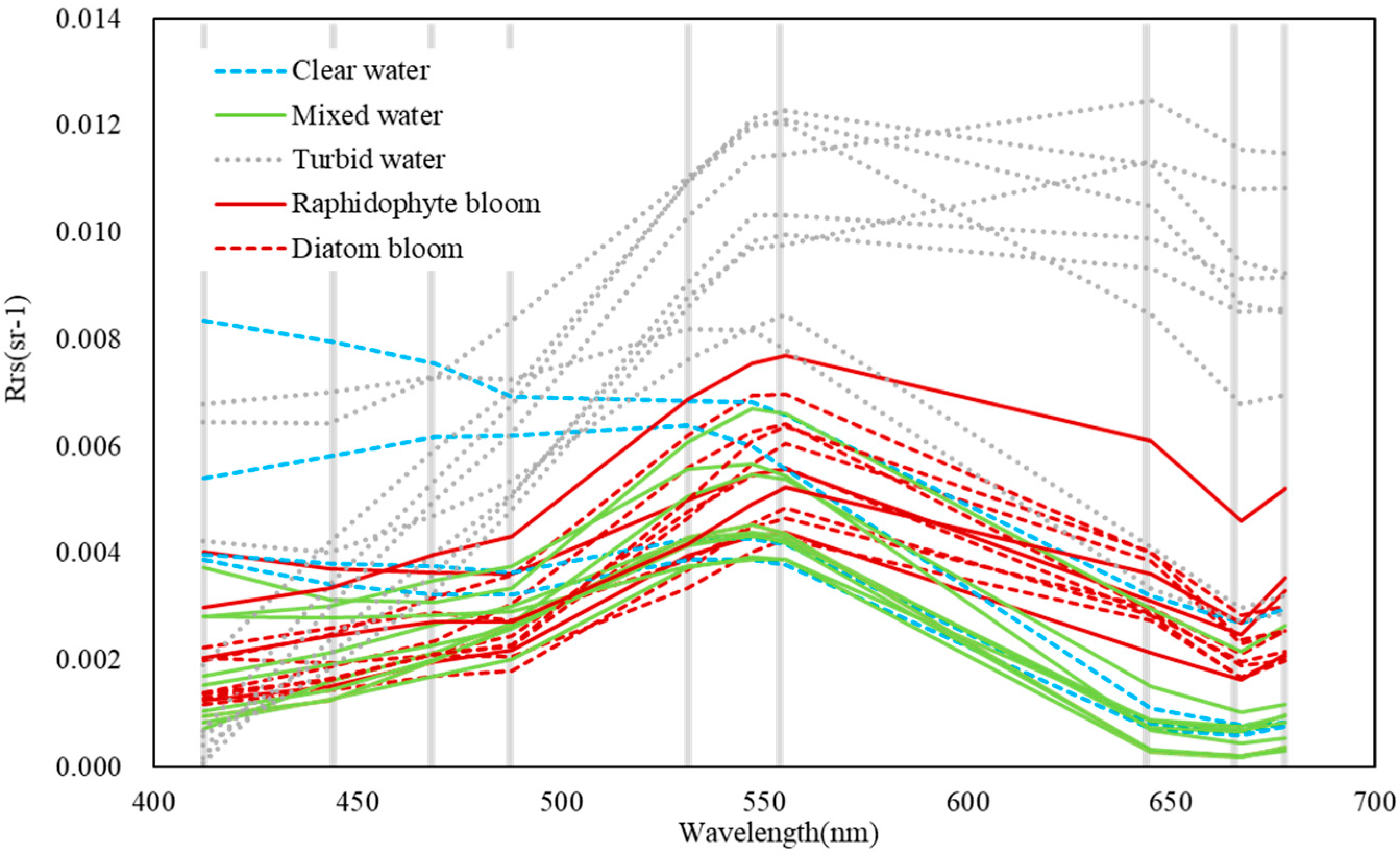
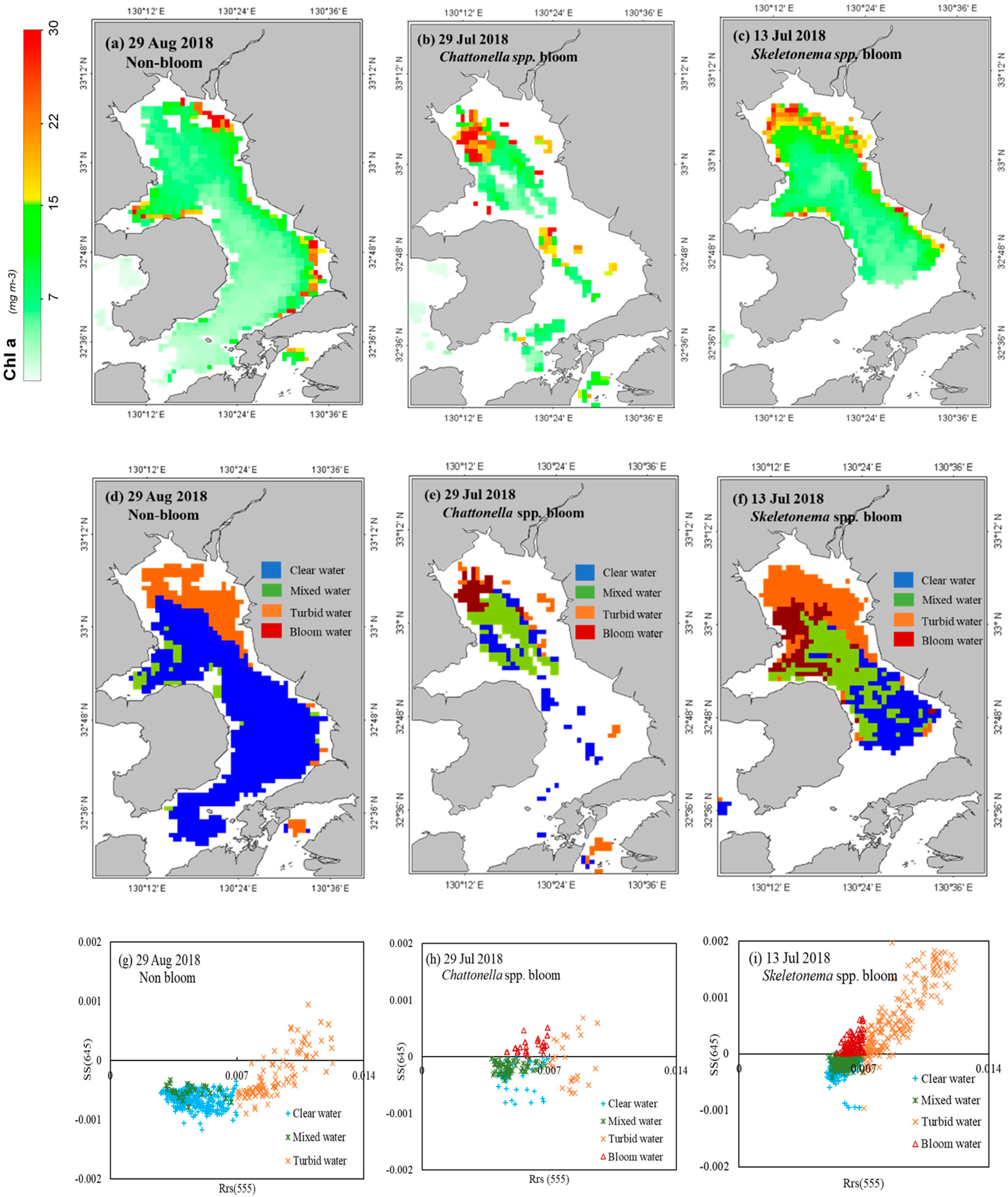
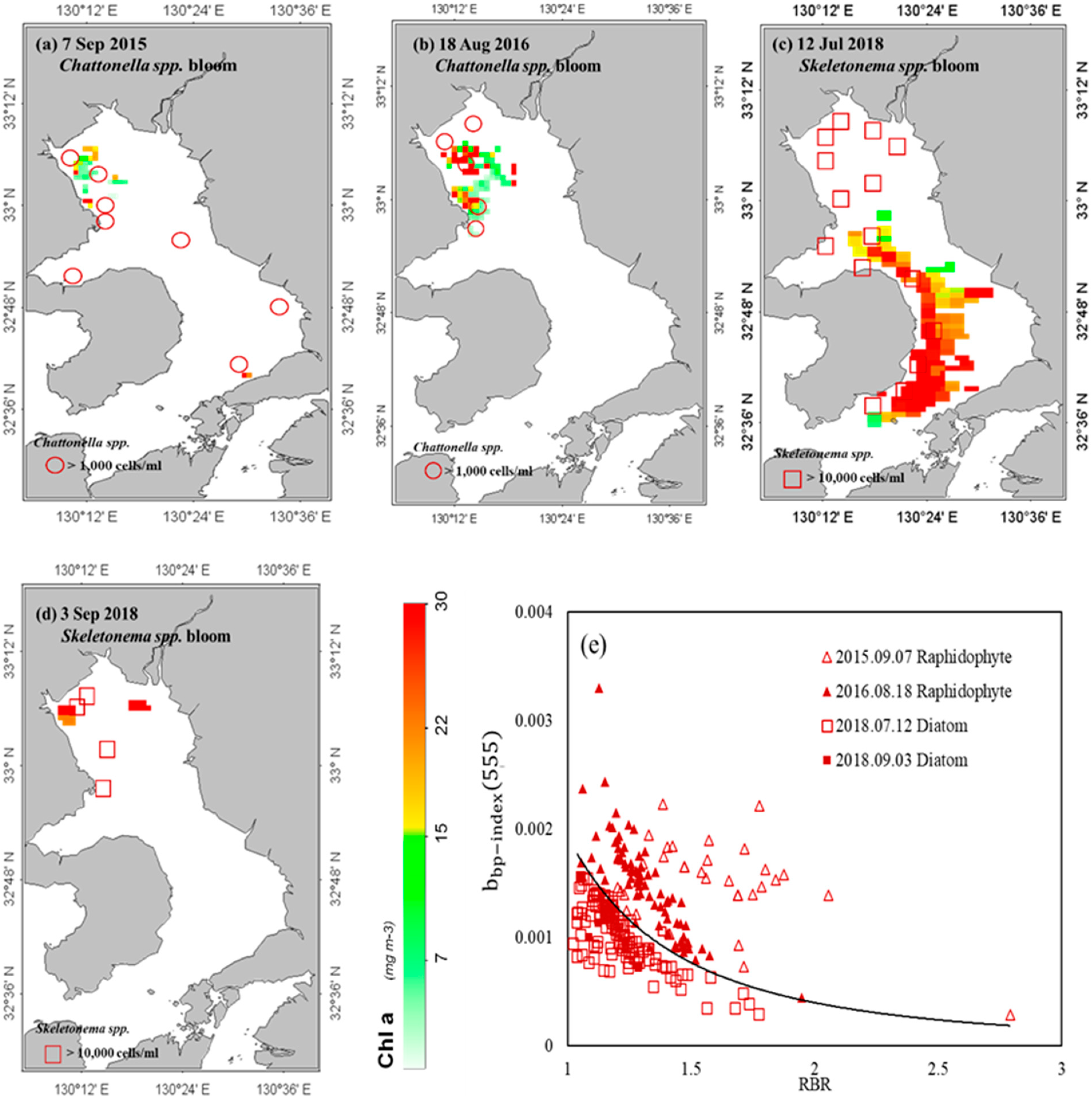
3.1. Detection of Bloom Waters

The first step was to correctly identify blooms from other optically dominant water types. MODIS $R_{rs}\left(\lambda \right)$ coincident with in-situ data showed considerable variability in both spectral shape and magnitude, indicating different water types in the observations (Figure 2). By comparing the spectral shape of $R_{rs}\left(\lambda \right)$ and Chl a concentrations for the three data groups (Table 1), the coastal area of Ariake Sea could be roughly separated into four bio-optical water types: (1) clear waters in the northeastern coast of Ariake Sea with low Chl a (<6.32 mg m⁻³), and relatively high blue reflectance compared to the longer wavelength green band where no peak was observed; (2) turbid waters within estuary area, which exhibited extremely high reflectance at longer wavelength because of the high suspended sediments; (3) bloom waters, typically located in the northwestern part of Ariake Sea with moderate to high Chl a, and a spectral shape of reflectance typical of phytoplankton blooms with minimal values in the blue region and high values near 550 nm and 678 nm; and (4) mixed water defined as water with a middle range of Chl a concentration and a peak in green bands.

Based on the differences observed, we could separate clear water if the $R_{rs}\left(\lambda \right)$ peak was at wavelengths shorter than 555 nm, and turbid water if the $R_{rs}\left(\lambda \right)$ peak was > 0.008 sr⁻¹. However, mixed waters with moderate Chl a concentration could not be separated from bloom waters based on this simple method since the former/latter also has a spectral peak at 555 nm (<0.008 sr⁻¹). So more detailed characteristics of the spectral shape were considered. Bloom waters showed prominent shoulders near 645 nm compared to mixed water (see Figure 2), which might be caused by strong backscattering of phytoplankton particles and weak absorption at this wavelength. To better characterize this feature, changes in the curvature of $R_{rs}\left(645\right)$ were compared to determine whether bloom waters could be distinguished from mixed water using this approach. The spectral shape algorithm (SS) of Wynne et al. [8], equivalent to the 2nd derivative when the bands are evenly distributed, provides an SS index which can describe the spectral variations useful in bloom detection [32,33]. In this study, normalized water leaving radiance ($n{L}_w$) is replaced with $R_{rs}\left(\lambda \right)$. The defined SS is as:

$$\mathrm{SS}\left(\mathsf{\lambda }\right)=R_{rs}\left(\lambda \right)-R_{rs}\left({\lambda }^{-}\right)-\left(R_{rs}\left({\lambda }^{+}\right)-R_{rs}\left({\lambda }^{-}\right)\right)\ast \frac{\left(\lambda -{\lambda }^{-}\right)}{\left({\lambda }^{+}-{\lambda }^{-}\right)},$$

(1)

where λ is the central band of the shape (645 nm), ${\lambda }^{-}$ is the next lower band (555 nm) and ${\lambda }^{+}$ is the next higher band (667 nm). SS (645) of bloom waters showed positive values while mixed waters exhibited negative values (Figure 3). Turbid water also showed positive SS (645), and was distinguishable by the threshold at $R_{rs}\left(555\right)$ (>0.008 sr⁻¹).

Together, algal bloom waters were differentiated from clear, turbid, and mixed waters by a combination of $R_{rs}\left(555\right)$ and SS (645). In the relationship between $R_{rs}\left(555\right)$ and SS (645) (Figure 3), clear and mixed waters were distinguished by negative SS (645) while bloom waters were identified by a positive SS (645) and low $R_{rs}\left(555\right)$ (<0.008 sr⁻¹). Even though turbid water also showed a positive SS (645), $R_{rs}\left(555\right)$ was higher than in bloom waters. The scatter plot shown in Figure 3 indicates that all observations with positive SS (645) and $R_{rs}\left(555\right)$ less than 0.008 sr⁻¹ could be characterized as algal bloom waters.

In order to verify the utility of satellite-derived SS (645) and $R_{rs}\left(555\right)$ for detecting blooms, three independent MODIS images were selected to coincide with summer bloom reports by the Japan Red Tide Online from 2015–2018: (a raphidophyte bloom on 29 July 2018; a diatom bloom on 13 July 2018; one non-bloom day on 29 August 2018). Scatter plot of satellite derived SS (645) versus $R_{rs}\left(555\right)$ is shown in Figure 4. The MODIS Chl a image in late summer on 29 August 2018, when no bloom event was reported in Ariake Sea, showed no sign of high Chl a in most of the area (Figure 4a). High values were seen only near Kumamoto coasts and Isahaya Bay. The corresponding scatter plot (Figure 4g) showed that the surface waters was roughly divided into clear, turbid and mixed waters. Conversely, relatively high Chl a was observed in the MODIS images (Figure 4b,c) in association with blooms of the raphidophyte (Chattonella spp.) and the diatom (Skeletonema spp.), which had been confirmed by field observations (Figure 4h,i).

It is to be noted that negative values of standard MODIS $R_{rs}\left(\lambda \right)$ at 412 nm and 645 nm were observed for pixels associated with high Chl a, and such high Chl a retrievals are inaccurate. Thus, for the bloom distinguishing method these pixels were excluded. Other than this limitation, the bloom distinguishing method can be applied to MODIS data and the combination of $R_{rs}\left(555\right)$ and SS (645) can serve as the first step to classify blooms from space.

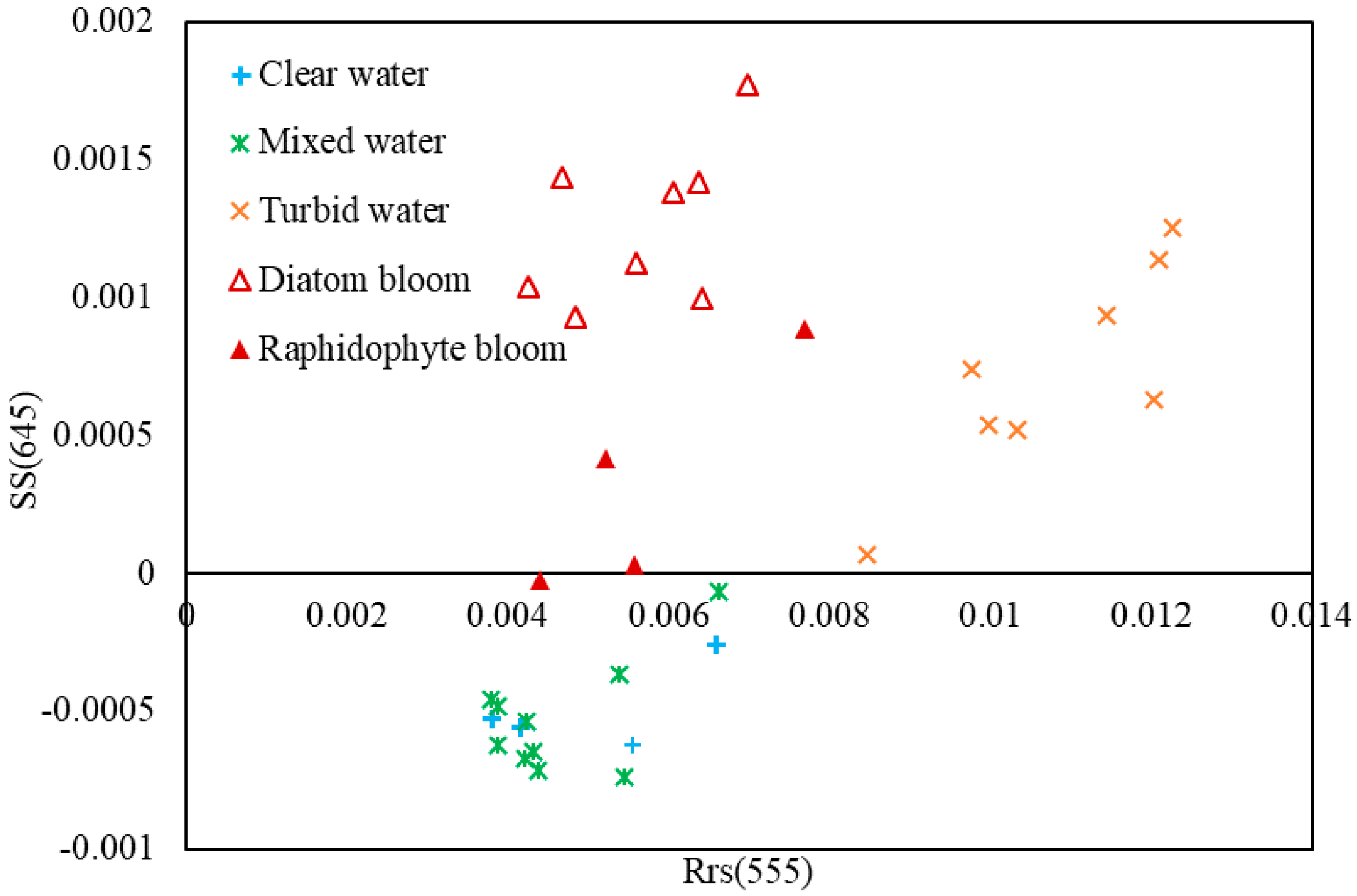
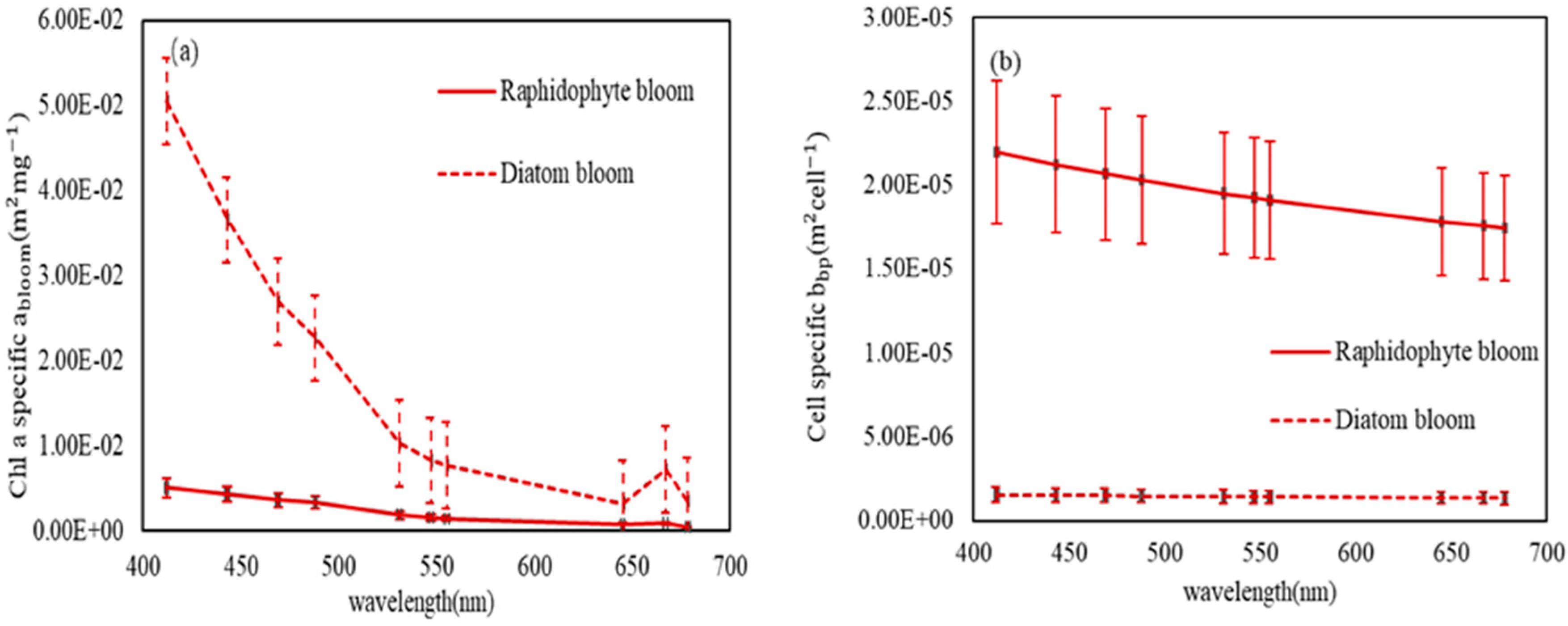
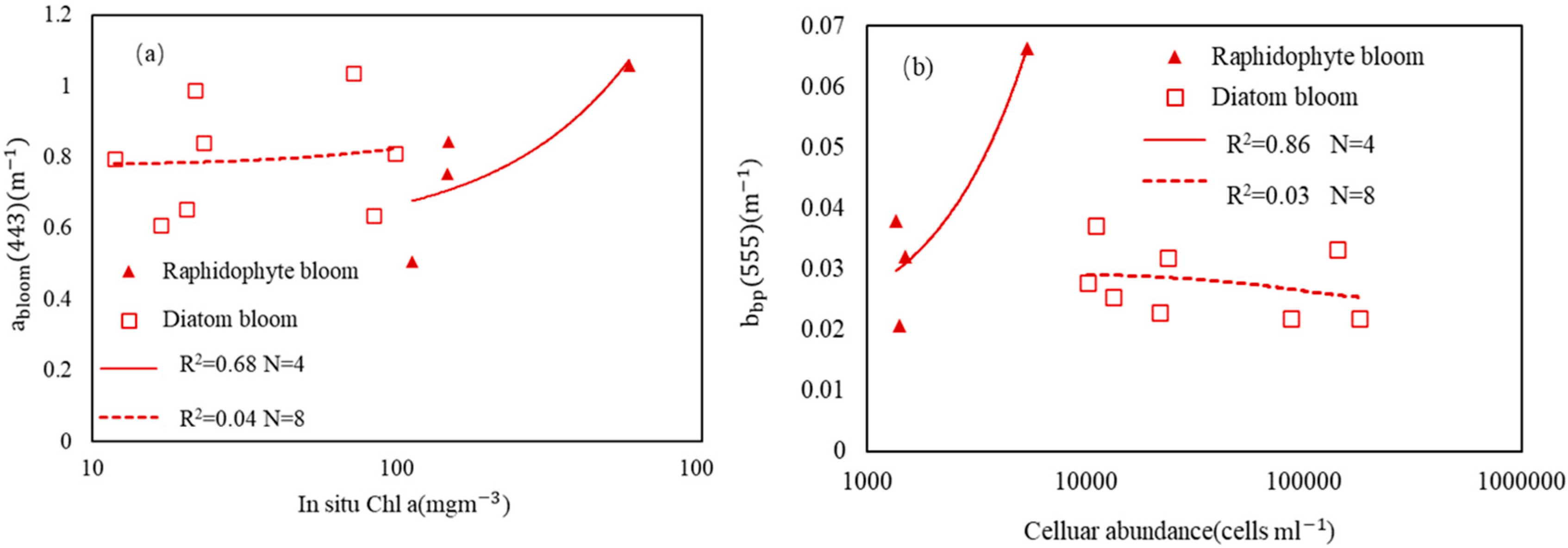
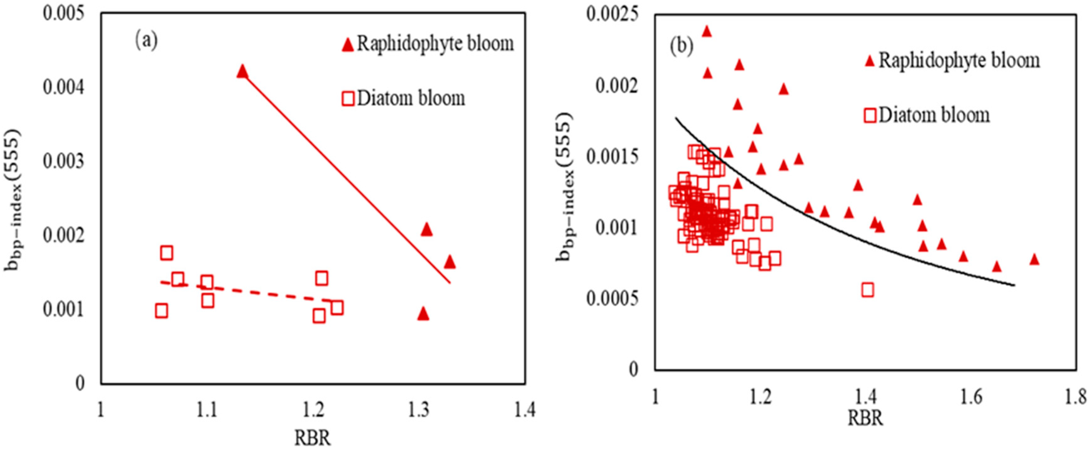
3.2. Discrimination of Harmful Algal Groups

To differentiate dominant algal blooms, inherent optical properties should be first compared. The spectral shape of $R_{rs}\left(\lambda \right)$ for bloom water is influenced by absorption and backscattering coefficients ($a_t\left(\mathsf{\lambda }\right)$, $b_b\left(\mathsf{\lambda }\right)$) [34,35]. They can be expressed as:

$$a_t\left(\mathsf{\lambda }\right)=a_w\left(\mathsf{\lambda }\right)+a_{dg}\left(\mathsf{\lambda }\right)+a_{ph}\left(\mathsf{\lambda }\right),$$

(2)

$$b_b\left(\mathsf{\lambda }\right)=b_{bw}\left(\mathsf{\lambda }\right)+b_{bp}\left(\mathsf{\lambda }\right),$$

(3)

where $a_w\left(\mathsf{\lambda }\right)$ and $b_{bw}\left(\mathsf{\lambda }\right)$ are the absorption and backscattering coefficients of pure water which are constants [36,37]. $a_{dg}\left(\mathsf{\lambda }\right)$ and $a_{ph}\left(\mathsf{\lambda }\right)$ represent non-algal and algal absorption, respectively. Non-algal absorption includes absorption by non-algal particles (NAP) and dissolved chromophoric dissolved organic matter (CDOM). $b_{bp}\left(\mathsf{\lambda }\right)$ is the suspended particle backscattering coefficient, and includes backscattering by phytoplankton and inorganic particles.

Ideally, if we could derive $a_{ph}\left(\mathsf{\lambda }\right)$ accurately by QAA, then we would be able to discriminate harmful algal species accurately. However, it has been shown that there is much uncertainty in partitioning $a_t\left(\mathsf{\lambda }\right)$ into $a_{ph}\left(\mathsf{\lambda }\right)$ and $a_{dg}\left(\mathsf{\lambda }\right)$ for high absorption waters [29,38]. During the bloom, except for absorption by water, both algal particles and non-algal particles influenced variations in $R_{rs}\left(\lambda \right)$ because of the optical complexity of coastal waters. So, here we assume that the variations in absorption by bloom waters can be represented as the difference between $a_t\left(\mathsf{\lambda }\right)$ and $a_w\left(\mathsf{\lambda }\right)$. To prevent confusion, we use:

$$a_{bloom}\left(\mathsf{\lambda }\right)=a_t\left(\mathsf{\lambda }\right)-a_w\left(\mathsf{\lambda }\right),$$

(4)

where $a_{bloom}\left(\mathsf{\lambda }\right)$ represent the absorption by bloom waters.

In addition, the contribution of $b_{bw}\left(\mathsf{\lambda }\right)$ was much smaller than suspended particle backscattering by bloom waters, and extremely high $b_{bp}\left(\mathsf{\lambda }\right)$ in turbid water was confirmed by the threshold of $R_{rs}\left(555\right)$ (>0.008 sr⁻¹). Additionally, previous studies have shown that the summer bloom occurs when the water column stratifies with higher nutrients and lower turbidity in the Ariake Sea [39,40,41]. Thus $b_{bp}$(λ) of bloom water was mainly contributed by organic matters rather than inorganic particles.

Figure 5 shows the Chl a-specific $a_{bloom}\left(\mathsf{\lambda }\right)$ and cell-specific $b_{bp}\left(\mathsf{\lambda }\right)$, as normalized to Chl a concentrations and cellular abundances, respectively. Both $a_{bloom}\left(\mathsf{\lambda }\right)$ and $b_{bp}\left(\mathsf{\lambda }\right)$ were derived from MODIS $R_{rs}\left(\lambda \right)$ by QAA V6. Figure 5a shows that the Chl a-specific absorption $a_{bloom}\left(\mathsf{\lambda }\right)$ for the raphidophyte bloom was lower than the diatom bloom, which might be caused by the higher intracellular pigment concentration of raphidophyte (Chattonella spp.) than that of the diatom (Skeletonema spp.). Chl a cell⁻¹ was 0.0811 for raphidophytes and 0.001 for diatoms. Additionally, when compared with longer wavelengths, there was large difference in the short bands, possibly due to variations in CDOM and NAP.

In contrast to $a_{bloom}\left(\mathsf{\lambda }\right)$, $b_{bp}\left(\mathsf{\lambda }\right)$ showed less spectral dependence (within 8%). The cell-specific $b_{bp}\left(\mathsf{\lambda }\right)$ of raphidophyte bloom water was about 10 times than that of the diatom bloom water. The difference in cell-specific $b_{bp}\left(\mathsf{\lambda }\right)$ can be attributed to cell size, cell shape, cell structure and particulate organic carbon content [42]. Specifically, the cell diameter of Chattonella spp. (raphidophyte) (30–100 μm) is 5 times that of Skeletonema spp. (diatom) (2–12 μm) and raphidophytes carbon content is much higher than that of diatoms [43,44,45]. Besides, Skeletonema spp. is a chain forming diatom while Chattonella spp. is present as single cells during a bloom, which may also be responsible for the backscattering feature.

To better understand the significance of the difference in Chl a-specific $a_{bloom}\left(\mathsf{\lambda }\right)$ and cellular-specific $b_{bp}\left(\mathsf{\lambda }\right)$ of Chattonella spp. and Skeletonema spp., we plotted the relationship between in situ Chl a and $a_{bloom}\left(443\right)$ because absorption from multiple components overlap at this band. Very little variation was found for the diatom bloom (R² = 0.004), whereas a trend (R² = 0.68) was observed for raphidophyte bloom waters (Figure 6). The former could have arisen because of lower Chl a concentration per unit cell and the package effect. Additionally, the invariant relationship between in situ Chl a and $a_{bloom}\left(443\right)$ in diatoms (Figure 6a) could have been due to absorbance in this band by CDOM and NAP. A similar pattern was also found in the relationship between cellular abundance and $b_{bp}\left(555\right)$. The $b_{bp}\left(555\right)$ of the raphidophyte bloom increased with cellular abundance (R² = 0.86) while that of the diatom bloom did not. This indicates lower backscattering per unit cell in the diatom bloom (Figure 6b). Based on the above, $b_{bp}\left(\mathsf{\lambda }\right)$ appears to be a better indicator to discriminate the two algal groups, especially considering the uncertainties associated with CDOM and NAP absorption in these coastal waters.

Therefore, based on Tao et al. [11], an index $b_{bp-index}\left(555\right)$ was developed using $R_{rs}\left(\lambda \right)$ from green to red bands to replace the QAA derived $b_{bp}\left(555\right)$, and thus avoiding the uncertainties associated with using the short waveband in QAA. The 555 nm waveband was chosen because both of NAP and water absorption is relatively low at this band [36].

It is known that $R_{rs}\left(\lambda \right)$ can be expressed in terms of absorption and backscattering [35,46]:

$$R_{rs}\left(\lambda \right)=\frac{f\left(\lambda \right)}{Q\left(\lambda \right)}\frac{b_b\left(\mathsf{\lambda }\right)}{a\left(\mathsf{\lambda }\right)+b_b\left(\mathsf{\lambda }\right)},$$

(5)

The $f\left(\lambda \right)$ refers to the irradiance reflectance within water while $Q\left(\lambda \right)$ describes the angular distribution of upwelling radiance, and their ratio is relatively stable [47]. Here we assume the $f\left(\lambda \right)/Q\left(\lambda \right)$ is spectrally invariant between 500 to 670 nm. From Equations (2) and (4), we can then derive the following relationship:

$$R_{rs}\left(\lambda \right)\propto \frac{f\left(\lambda \right)}{Q\left(\lambda \right)}\frac{b_{bp}\left(\mathsf{\lambda }\right)}{a_w\left(\mathsf{\lambda }\right)+a_{bloom}\left(\mathsf{\lambda }\right)+b_{bp}\left(\mathsf{\lambda }\right)},$$

(6)

Figure 5a shows that the difference in $a_{bloom}\left(\mathsf{\lambda }\right)$ between 555 and 667 nm was very small. Thus, the following assumption can be made for each species:

$$a_{bloom}\left(555\right)=a_{bloom}\left(667\right),$$

(7)

Additionally, the spectral dependence of $b_{bp}\left(\mathsf{\lambda }\right)$ was small, and it showed only a small variation, within 8% (Figure 5b). So $b_{bp}\left(\mathsf{\lambda }\right)$ was assumed to be equal at bands 555 and 667 nm:

$$b_{bp}\left(555\right)=b_{bp}\left(667\right),$$

(8)

Finally, $b_{bp}\left(555\right)$ was derived from Equation (5) using the reciprocal of $R_{rs}\left(\lambda \right)$ at 555 and 667 nm, as:

$$\frac{1}{R_{rs}\left(667\right)}-\frac{1}{R_{rs}\left(555\right)}\propto \frac{a_w\left(667\right)-a_w\left(555\right)}{b_{bp}\left(555\right)},$$

(9)

where $a_w\left(667\right)-a_w\left(555\right)$ = 0.37 m⁻¹. The variations in $b_{bp}\left(555\right)$ can thus be expressed by the variations in $R_{rs}\left(\lambda \right)$ at 555 and 667 nm:

$$b_{bp}\left(555\right)\propto 0.37\times \frac{R_{rs}\left(555\right)R_{rs}\left(667\right)}{R_{rs}\left(555\right)-R_{rs}\left(667\right)}=b_{bp-index}\left(555\right),$$

(10)

To differentiate from $b_{bp}\left(555\right)$, henceforth we use $b_{bp-index}\left(555\right)$ described in the equation above.

Although bloom vs. non-bloom conditions could be detected by the positive SS (645) (Section 3.1), it was not possible to differentiate between raphidophyte and diatom blooms based on the combination of SS (645) and $b_{bp-index}\left(555\right)$. Considering the difference in magnitude of Chl a concentrations during the two blooms, a supplementary index, the Red Band Ratio (RBR) that accounts for Chl a concentrations was used to identify algal types. RBR utilizes the ratio of $R_{rs}\left(678\right)$ and $R_{rs}\left(667\right)$ to describe the high fluorescence emission around red bands caused by Chl a [48]. The ratio is characterized as:

$$\mathrm{R}\mathrm{BR}=\frac{R_{rs}\left(678\right)}{R_{rs}\left(667\right)},$$

(11)

The two algal species were thus classified by the distribution of $b_{bp-index}\left(555\right)$ and the RBR for MODIS data collocated with field data (Figure 7a). For a given RBR value, the raphidophyte blooms showed higher $b_{bp-index}\left(555\right)$ than diatom blooms. Figure 7b presents a more distinct relationship between $b_{bp-index}\left(555\right)$ and RBR using the independent MODIS $R_{rs}\left(\lambda \right)$ data shown in Figure 4b,c for bloom waters. Although some raphidophyte points overlapped with diatoms, the plot shows two distinct relationships for raphidophytes and diatoms. An exponential curve was fit to the data (Figure 7b), which can be expressed as:

$$b_{bp-index}\left(555\right)=0.0019RB{R}^{-2.261}$$

(12)

Accordingly, a bloom can be classified as a raphidophyte (Chattonella spp.) bloom if the $b_{bp-index}\left(555\right)$ is higher than the value calculated from the RBR value using Equation (12), and conversely as a diatom (Skeletonema spp.) bloom if it $b_{bp-index}\left(555\right)$ is lower than that calculated from the RBR value.

MODIS images from 2015 to 2018 were examined to verify the discrimination between raphidophyte and diatom blooms, using the independent data of bloom reports from Japan Red Tide Online. It included the raphidophyte (Chattonella spp.) blooms on 7 September 2015 and 18 August 2016 (Figure 8a,b), and the diatom (Skeletonema spp.) blooms occurred on 12 July 2018 and 3 September 2018 (Figure 8c,d). The corresponding scatter plot of $b_{bp-index}\left(555\right)$ and RBR is shown in Figure 8e. It confirmed that the combination of $b_{bp-index}\left(555\right)$ and RBR could successfully distinguish raphidophyte blooms from diatom blooms in MODIS images.

4. Discussion

The outline of the new method proposed in this study, which can distinguish raphidophyte blooms, diatom blooms, and non-bloom waters in the Ariake Sea, is illustrated in Figure 9. The method is simple, but effective, in discriminating harmful algal blooms, and it does offer several novel findings over previous studies.

It is widely known that phytoplankton blooms are associated with high Chl a concentration and a peak in $R_{rs}\left(\lambda \right)$ in the green band [2,16,49], but our method shows that high Chl a using the standard MODIS algorithm is not always related to blooms (Figure 4a–f and Figure 8a–d). Many previous methods detect harmful blooms based on the peak at 555 nm of satellite derived $R_{rs}\left(\lambda \right)$ [7,50,51]. However, both sediments and CDOM might influence the accuracy of $R_{rs}\left(\lambda \right)$ at the green peak observed by satellite, as well as inaccurate atmospheric correction in coastal waters [23,24,25] which may make the peak in the green bands and satellite retrieved Chl a concentrations unreliable for bloom detection. A suitable local-based atmosphere correction is needed to overcome the uncertainty in short bands. Our novel method captured the unique $R_{rs}\left(\lambda \right)$ shoulder at 645 nm in bloom waters, which successfully distinguished raphidophyte and diatom blooms in the Ariake Sea. Although this method used $R_{rs}\left(555\right)$ in the SS (645) calculation, it was used only as a baseline to describe the spectral shape of $R_{rs}\left(\lambda \right)$ at 645 nm rather than as the dominant component, thus the uncertainty in SS (645) can be much smaller than the green band based algorithm. Compared with previous studies, our method detects harmful blooms effectively using the spectral features at longer wavelengths and without the uncertainty of short bands.

The 645 nm shoulder of $R_{rs}\left(\lambda \right)$ might be influenced by low Chl a and backscattering of algal particles [52], which means pigment absorption is weak around 645 nm, and algal particle backscatter dominated the $R_{rs}\left(\lambda \right)$. Mixed water was influenced strongly by water absorption at 645 nm, which results in negative values of SS (645) even though there is a peak in the green band. Although turbid waters also show a spectral shoulder at 645 nm, which is caused by the strong scattering by non-algal particles, we can exclude it by placing a threshold for $R_{rs}\left(555\right)$. This newly developed method can detect the bloom precisely and provide accurate information related to areas where blooms are occurring.

Many studies have been developed to use applied inherent optical properties to distinguish harmful algal species [10,11,12,53]. Even though these studies showed excellent results for their study regions, it has not been applicable to other regions such as the Ariake Sea (results were not show here). One reason might be differences in water conditions. FLH or Chl a concentration is needed as a precondition in methods like those of Cannizzaro et al. [12,53] and Shang et al. [28] to constrain the use of the developed bloom index ($b_{bp}\left(\mathsf{\lambda }\right)$ ratio and bloom index (BI), respectively), which may vary for different regions. The Green–Red Index of Tao et al. [11] did not work for the Ariake Sea probably because of the different pigment composition of algal species. Although both the East China Sea (ECS) and the Ariake Sea are dominated by phytoplankton groups like diatoms and flagellates [15,54,55], the species can be very different. Consequently, one method which works well in one place may not work in other locations.

Existing methods have not been successful in discriminating raphidophytes, the more common, non-diatom, bloom forming organism in the Ariake Sea, from diatoms, while the newly developed method in the present study showed potential for algal species distinction. Considering the frequent and alternately occurring diatom and raphidophytes HABs in the Ariake Sea, our method is highly advantageous as it is able to discriminate Chattonella spp. and Skeletonema spp. blooms. As can be seen in Figure 8a–b, the newly developed method captured the blooms on 7 September 2015 and 18 August 2016, and this was in accord with the field observations on the day, which showed cells count of >1000 cells mL⁻¹ of Chattonella spp. The MODIS pixels indicated as algal blooms were classified as Chattonella spp. blooms in the scatter plot of Figure 8e. In Figure 8c–d, the blooms captured in the MODIS image of 12 July 2018 and 3 September 2018 were confirmed to contain high concentrations of Skeletonema spp. cells as per local bloom reports. Accordingly, pixels from the bloom areas were classified as diatom blooms as shown in Figure 8e. In spite of the lack of in situ measurements of inherent optical properties, the exciting results in Figure 8e encourage us to pay more attention to backscattering features in harmful algae discrimination in the future. This demonstrates how backscattering can be used in combination with Chl a for bloom detection and harmful algal discrimination.

In summary, our method has several advantages over previous methods. This method can be used directly on MODIS $R_{rs}\left(\lambda \right)$ products. Additionally, satellite short waveband data was excluded to avoid possible errors arising from incorrect atmospheric corrections and the influence of non-phytoplankton particles.

5. Conclusions

A novel multispectral approach using MODIS-derived $R_{rs}\left(\lambda \right)$ and based on an algal backscattering feature was developed to detect raphidophyte and diatom blooms in the Ariake Sea. As a first step, this method uses the $R_{rs}\left(\lambda \right)$ spectral shape signature in the red band to detect HABs. The bloom waters are successfully differentiated by a positive SS (645) and the water can be divided into clear, turbid, mixed and bloom waters. For the next step, indices of $b_{bp-index}\left(555\right)$ were developed and used with RBR for discriminating raphidophyte and diatom blooms, based on the distinct optical properties of backscattering between the two algal species. Comparison with the red tide report in 2015–2018 showed that this new method could provide reliable spatial distribution of the raphidophyte and diatom blooms, which may provide a better understanding of harmful algal bloom distributions in the Ariake Sea.

Since the coastal environment is optically complex and varies temporally, more field measurements are needed to better understand the unique backscattering feature that allowed us to distinguish Chattonella spp. from Skeletonema spp. blooms. Moreover, additional efforts are required to apply this method to other coastal areas with similar algal constituents. Besides, satellites like GOCI and GCOM-C will be utilized in the future to check its applicability for investigation high temporal variability of these blooms over larger areas.

References

1. Xi, H.; Hieronymi, M.; Röttgers, R.; Krasemann, H.; Qiu, Z. Hyperspectral differentiation of phytoplankton taxonomic groups: A comparison between using remote sensing reflectance and absorption spectra. Remote Sens. 2015, 7, 14781–14805. [Google Scholar] [CrossRef] [Green Version]
2. Gower, J.; King, S.; Goncalves, P. Global monitoring of plankton blooms using MERIS MCI. Int. J. Remote Sens. 2008, 29, 6209–6216. [Google Scholar] [CrossRef]
3. Shanmugam, P. A new bio-optical algorithm for the remote sensing of algal blooms in complex ocean waters. J. Geophys. Res. Oceans 2011, 116. [Google Scholar] [CrossRef] [Green Version]
4. Hu, C. A novel ocean color index to detect floating algae in the global oceans. Remote Sens. Environ. 2009, 113, 2118–2129. [Google Scholar] [CrossRef]
5. Westberry, T.; Siegel, D.; Subramaniam, A. An improved bio-optical model for the remote sensing of Trichodesmium spp. blooms. J. Geophys. Res. Oceans 2005, 110. [Google Scholar] [CrossRef] [Green Version]
6. Amin, R.; Zhou, J.; Gilerson, A.; Gross, B.; Moshary, F.; Ahmed, S. Novel optical techniques for detecting and classifying toxic dinoflagellate Karenia brevis blooms using satellite imagery. Opt. Express 2009, 17, 9126–9144. [Google Scholar] [CrossRef]
7. Noh, J.H.; Kim, W.; Son, S.H.; Ahn, J.H.; Park, Y.J. Remote quantification of Cochlodinium polykrikoides blooms occurring in the East Sea using geostationary ocean color imager (GOCI). Harmful Algae 2018, 73, 129–137. [Google Scholar] [CrossRef]
8. Wynne, T.; Stumpf, R.; Tomlinson, M.; Warner, R.; Tester, P.; Dyble, J.; Fahnenstiel, G. Relating spectral shape to cyanobacterial blooms in the Laurentian Great Lakes. Int. J. Remoe Sens. 2008, 29, 3665–3672. [Google Scholar] [CrossRef]
9. Siswanto, E.; Ishizaka, J.; Tripathy, S.C.; Miyamura, K. Detection of harmful algal blooms of Karenia mikimotoi using MODIS measurements: A case study of Seto-Inland Sea, Japan. Remote Sens. Environ. 2013, 129, 185–196. [Google Scholar] [CrossRef]
10. Shang, S.; Wu, J.; Huang, B.; Lin, G.; Lee, Z.; Liu, J.; Shang, S. A new approach to discriminate dinoflagellate from diatom blooms from space in the East China Sea. J. Geophys. Res. Oceans 2014, 119, 4653–4668. [Google Scholar] [CrossRef]
11. Tao, B.; Mao, Z.; Lei, H.; Pan, D.; Bai, Y.; Zhu, Q.; Zhang, Z. A semianalytical MERIS green-red band algorithm for identifying phytoplankton bloom types in the East China Sea. J. Geophys. Res. Oceans 2017, 122, 1772–1788. [Google Scholar] [CrossRef]
12. Cannizzaro, J.P.; Carder, K.L.; Chen, F.R.; Heil, C.A.; Vargo, G.A. A novel technique for detection of the toxic dinoflagellate, Karenia brevis, in the Gulf of Mexico from remotely sensed ocean color data. Cont. Shelf Res. 2008, 28, 137–158. [Google Scholar] [CrossRef]
13. Burenkov, V.; Kopelevich, O.; Rat’kova, T.; Sheberstov, S. Satellite observations of the coccolithophorid bloom in the Barents Sea. Oceanology 2011, 51, 766. [Google Scholar] [CrossRef]
14. Lei, H.; Pan, D.; Bai, Y.; Chen, X.; Zhou, Y.; Zhu, Q. HAB detection based on absorption and backscattering properties of phytoplankton. In Proceedings of the Remote Sensing of the Ocean, Sea Ice, Coastal Waters, and Large Water Regions 2011, Prague, Czech Republic, 19–22 September 2011; p. 81751F. [Google Scholar]
15. Ishizaka, J.; Kitaura, Y.; Touke, Y.; Sasaki, H.; Tanaka, A.; Murakami, H.; Suzuki, T.; Matsuoka, K.; Nakata, H. Satellite detection of red tide in Ariake Sound, 1998–2001. J. Oceanogr. 2006, 62, 37–45. [Google Scholar] [CrossRef]
16. Sasaki, H.; Tanaka, A.; Iwataki, M.; Touke, Y.; Siswanto, E.; Tan, C.K.; Ishizaka, J. Optical properties of the red tide in Isahaya Bay, southwestern Japan: Influence of chlorophyll a concentration. J. Oceanogr. 2008, 64, 511–523. [Google Scholar] [CrossRef]
17. Aoki, K.; Onitsuka, G.; Shimizu, M.; Yamatogi, T.; Ishida, N.; Kitahara, S.; Hirano, K. Chattonella (Raphidophyceae) bloom spatio-temporal variations in Tachibana Bay and the southern area of Ariake Sea, Japan: Interregional displacement patterns with Skeletonema (Bacillariophyceae). Mar. Pollut. Bull. 2015, 99, 54–60. [Google Scholar] [CrossRef]
18. Khan, S.; Arakawa, O.; Onoue, Y. A toxicological study of the marine phytoflagellate, Chattonella antiqua (Raphidophyceae). Phycologia 1996, 35, 239–244. [Google Scholar] [CrossRef]
19. Andreae, M.O.; Klumpp, D. Biosynthesis and release of organoarsenic compounds by marine algae. Environ. Sci. Technol. 1979, 13, 738–741. [Google Scholar] [CrossRef]
20. Howard, A.; Comber, S.; Kifle, D.; Antai, E.; Purdie, D. Arsenic speciation and seasonal changes in nutrient availability and micro-plankton abundance in Southampton water, UK. Estuar. Coast. Shelf Sci. 1995, 40, 435–450. [Google Scholar] [CrossRef]
21. Imai, I. Distribution of diatom resting cells in sediments of Harima-Nada and northern Hiroshima Bay, the Seto Inland Sea, Japan. Bull. Coast Oceanogr. 1990, 28, 75–84. [Google Scholar]
22. Azad, M.A.K.; Ohira, S.-I.; Oda, M.; Toda, K. On-site measurements of hydrogen sulfide and sulfur dioxide emissions from tidal flat sediments of Ariake Sea, Japan. Atmos. Environ. 2005, 39, 6077–6087. [Google Scholar]
23. Zhang, M.; Carder, K.; Muller-Karger, F.E.; Lee, Z.; Goldgof, D.B. Noise reduction and atmospheric correction for coastal applications of Landsat Thematic Mapper imagery. Remote Sens. Environ. 1999, 70, 167–180. [Google Scholar] [CrossRef]
24. Hu, C.; Muller-Karger, F.E.; Andrefouet, S.; Carder, K.L. Atmospheric correction and cross-calibration of LANDSAT-7/ETM+ imagery over aquatic environments: A multiplatform approach using SeaWiFS/MODIS. Remote Sens. Environ. 2001, 78, 99–107. [Google Scholar] [CrossRef]
25. Yang, M.M.; Ishizaka, J.; Goes, J.I.; Gomes, H.d.R.; Maúre, E.D.R.; Hayashi, M.; Katano, T.; Fujii, N.; Saitoh, K.; Mine, T. Improved MODIS-Aqua chlorophyll-a retrievals in the turbid semi-enclosed Ariake Bay, Japan. Remote Sens. 2018, 10, 1335. [Google Scholar] [CrossRef] [Green Version]
26. Majchrowski, R.; Ostrowska, M.A. Influence of photo-and chromatic acclimation on pigment composition in the sea. Oceanologia 2000, 42, 157–175. [Google Scholar]
27. Bricaud, A.; Claustre, H.; Ras, J.; Oubelkheir, K. Natural variability of phytoplanktonic absorption in oceanic waters: Influence of the size structure of algal populations. J. Geophys. Res. Oceans 2004, 109. [Google Scholar] [CrossRef]
28. Lee, Z.; Huot, Y. On the non-closure of particle backscattering coefficient in oligotrophic oceans. Opt. Express 2014, 22, 29223–29233. [Google Scholar] [CrossRef] [Green Version]
29. Lee, Z.; Carder, K.L.; Arnone, R.A. Deriving inherent optical properties from water color: A multiband quasi-analytical algorithm for optically deep waters. Appl. Opt. 2002, 41, 5755–5772. [Google Scholar] [CrossRef]
30. Ronald, J.; Zaneveld, V. Remotely sensed reflectance and its dependence on vertical structure: A theoretical derivation. Appl. Opt. 1982, 21, 4146–4150. [Google Scholar] [CrossRef] [Green Version]
31. Jerome, J.; Bukata, R.; Miller, J. Remote sensing reflectance and its relationship to optical properties of natural waters. Remote Sens. 1996, 17, 3135–3155. [Google Scholar] [CrossRef]
32. Stumpf, R.P.; Wynne, T.T.; Baker, D.B.; Fahnenstiel, G.L. Interannual variability of cyanobacterial blooms in Lake Erie. PLoS ONE 2012, 7, e42444. [Google Scholar] [CrossRef] [PubMed]
33. Soto, I.M.; Cannizzaro, J.; Muller-Karger, F.E.; Hu, C.; Wolny, J.; Goldgof, D. Evaluation and optimization of remote sensing techniques for detection of Karenia brevis blooms on the West Florida Shelf. Remote Sens. Environ. 2015, 170, 239–254. [Google Scholar] [CrossRef]
34. Morel, A.; Prieur, L. Analysis of variations in ocean color 1. Limnol. Oceanogr. 1977, 22, 709–722. [Google Scholar] [CrossRef]
35. Gordon, H.R.; Brown, O.B.; Evans, R.H.; Brown, J.W.; Smith, R.C.; Baker, K.S.; Clark, D.K. A semianalytic radiance model of ocean color. J. Geophys. Res. Atmos. 1988, 93, 10909–10924. [Google Scholar] [CrossRef]
36. Pope, R.M.; Fry, E.S. Absorption spectrum (380–700 nm) of pure water. II. Integrating cavity measurements. Appl. Opt. 1997, 36, 8710–8723. [Google Scholar] [CrossRef]
37. Morel, A. Optical properties of pure water and pure sea water. Opt. Asp. Oceanogr. 1974, 1, 1–24. [Google Scholar]
38. Lee, Z.; Arnone, R.; Hu, C.; Werdell, P.J.; Lubac, B. Uncertainties of optical parameters and their propagations in an analytical ocean color inversion algorithm. Appl. Opt. 2010, 49, 369–381. [Google Scholar] [CrossRef]
39. Tanaka, K.; Kodama, M. Effects of resuspended sediments on the environmental changes in the inner part of Ariake Bay, Japan. Bull. Fish. Res. Agency Jpn. 2007, 19, 9. [Google Scholar]
40. Imai, I.; Yamaguchi, M. Life cycle, physiology, ecology and red tide occurrences of the fish-killing raphidophyte Chattonella. Harmful Algae 2012, 14, 46–70. [Google Scholar] [CrossRef]
41. Arai, K. Prediction Method for Large Diatom Appearance with Meteorological Data and MODIS Derived Turbidity and Chlorophyll-A in Ariake Bay Area in Japan. Inter. J. Adv. Comput. Sci. Appl. 2017, 8, 39–44. [Google Scholar] [CrossRef] [Green Version]
42. Vaillancourt, R.D.; Brown, C.W.; Guillard, R.R.; Balch, W.M. Light backscattering properties of marine phytoplankton: Relationships to cell size, chemical composition and taxonomy. J. Plankton Res. 2004, 26, 191–212. [Google Scholar] [CrossRef]
43. Tomas, C.R. Identifying Marine Phytoplankton; Elsevier: Amsterdam, The Netherlands, 1997. [Google Scholar]
44. Strathmann, R.R. Estimating the organic carbon content of phytoplankton from cell volume or plasma volume 1. Limnol. Oceanogr. 1967, 12, 411–418. [Google Scholar] [CrossRef]
45. Menden-Deuer, S.; Lessard, E.J. Carbon to volume relationships for dinoflagellates, diatoms, and other protist plankton. Limnol. Oceanogr. 2000, 45, 569–579. [Google Scholar] [CrossRef] [Green Version]
46. Carder, K.L.; Chen, F.; Lee, Z.; Hawes, S.; Kamykowski, D. Semianalytic Moderate-Resolution Imaging Spectrometer algorithms for chlorophyll a and absorption with bio-optical domains based on nitrate-depletion temperatures. Limnol. Oceanogr. 1999, 104, 5403–5421. [Google Scholar]
47. Morel, A.; Gentili, B. Diffuse reflectance of oceanic waters. II. Bidirectional aspects. Appl. Opt. 1993, 32, 6864–6879. [Google Scholar] [CrossRef]
48. Gitelson, A. The peak near 700 nm on radiance spectra of algae and water: Relationships of its magnitude and position with chlorophyll concentration. Int. J. Remote Sens. 1992, 13, 3367–3373. [Google Scholar] [CrossRef]
49. Hu, C.; Muller-Karger, F.E.; Taylor, C.J.; Carder, K.L.; Kelble, C.; Johns, E.; Heil, C.A. Red tide detection and tracing using MODIS fluorescence data: A regional example in SW Florida coastal waters. Remote Sens. Environ. 2005, 97, 311–321. [Google Scholar] [CrossRef]
50. Ahn, Y.-H.; Shanmugam, P.; Ryu, J.-H.; Jeong, J.-C. Satellite detection of harmful algal bloom occurrences in Korean waters. Harmful Algae 2006, 5, 213–231. [Google Scholar] [CrossRef]
51. Lou, X.; Hu, C. Diurnal changes of a harmful algal bloom in the East China Sea: Observations from GOCI. Remote Sens. Environ. 2014, 140, 562–572. [Google Scholar] [CrossRef]
52. Hoepffner, N.; Sathyendranath, S. Effect of pigment composition on absorption properties of phytoplankton. Mar. Ecol. Prog. Ser 1991, 73, 11–23. [Google Scholar] [CrossRef]
53. Cannizzaro, J.P. Detection and Quantification of Karenia brevis Blooms on the West Florida Shelf from Remotely Sensed Ocean Color Imagery. Master’s Thesis, University of South Florida, Tampa, FL, USA, 2004. [Google Scholar]
54. Tsutsumi, H. Critical events in the Ariake Bay ecosystem: Clam population collapse, red tides, and hypoxic bottom water. Plankton Benthos Res. 2006, 1, 3–25. [Google Scholar] [CrossRef] [Green Version]
55. Tao, B.; Mao, Z.; Lei, H.; Pan, D.; Shen, Y.; Bai, Y.; Zhu, Q.; Li, Z. A novel method for discriminating Prorocentrum donghaiense from diatom blooms in the East China Sea using MODIS measurements. Remote Sens. Environ. 2015, 158, 267–280. [Google Scholar] [CrossRef]
Figure 1. Map of Ariake Sea, Japan. Solid points show the field sampling locations in 2011–2014. The gray circle and square indicate the position of data taken by Saga Fisheries Promotion Center and Kumamoto Fisheries Research Center, respectively.
Remotesensing 12 01504 g001
Figure 2. MODIS R r s ( λ ) spectra (N = 35) using the match-up method (See Section 2.3). Blue dashed line (clear water); green solid line (mixed waters); gray dotted line (turbid water), red solid and dashed line indicates raphidophyte and diatom bloom water, respectively. The gray lines indicate location of MODIS bands.
Remotesensing 12 01504 g002
Figure 3. Scatter plot of MODIS R r s ( 555 ) and SS (645) generated based on the MODIS match-up pairs.
Remotesensing 12 01504 g003
Figure 4. (ac) Standard Chl a images from MODIS level-2 for Ariake Sea. Non-bloom (a), raphidophyte bloom (b) and diatom bloom (c) as confirmed by bloom reports from Japan Red Tide Online. (df) Water types derived using MODIS R r s ( λ ) and our newly developed method. (gi) Scatter plot of R r s ( 555 ) and SS (645) derived from the MODIS R r s ( λ ) extracted from scenes shown in (ac). Only areas with positive R r s ( λ ) are shown.
Remotesensing 12 01504 g004
Figure 5. Inherent optical properties of diatom and raphidophyte bloom waters: (a) Chl a-specific absorption of bloom water a b l o o m ( λ ) where a b l o o m ( λ ) is normalized to in situ Chl a concentration; (b) Cell-specific backscattering of suspended particles b b p ( λ ) . The spectra are normalized to cellular abundance. The a b l o o m ( λ ) and b b p ( λ ) were derived by the MODIS R r s ( λ ) match up results using QAA V6. N = 4 for raphidophyte bloom and N = 8 for diatom bloom. The solid and plot line represent raphidophyte and diatom bloom, respectively.
Remotesensing 12 01504 g005
Figure 6. (a) Scatterplot of in situ Chl a and a b l o o m ( 443 )   of the raphidophyte and diatom blooms; (b) scatterplot of cellular abundance and b b p ( 555 ) . The triangles and squares depict raphidophyte (N = 4) and diatom bloom (N = 8), respectively. Linear regression line was drawn on log transformed data. The data was from the match-up pairs of MODIS in 2011–2014. The a b l o o m ( 443 ) and b b p ( 555 ) were derived from MODIS R r s ( λ ) by QAA V6.
Remotesensing 12 01504 g006
Figure 7. (a) Scatter plot of RBR and b b p i n d e x ( 555 ) using MODIS R r s ( λ ) coincident with field data for 2011–2014. (b) Scatter plot of RBR and b b p i n d e x ( 555 ) derived from the points flagged as bloom in Figure 4b,c. The solid line in Figure 7b represents the function expressed by Equation (12) separating raphidophyte blooms from diatom blooms.
Remotesensing 12 01504 g007
Figure 8. (ad) MODIS Chl a images from standard level_2 products showing bloom distribution confirmed by reports from Japan Red Tide Online. Only pixels positively flagged as bloom waters are shown in color. The red circles and squares indicate the location of raphidophyte and diatom blooms, respectively. (e) Scatterplot of b b p i n d e x (555) and RBR derived from the bloom pixels in (ad), indicating distinct algal groups. Red triangle and squares indicate raphidophyte and diatom blooms, respectively.
Remotesensing 12 01504 g008
Figure 9. Multispectral method for the identification of raphidophyte and diatom, and non-bloom waters.
Remotesensing 12 01504 g009