Article

Mapping Seasonal Tree Canopy Cover and Leaf Area Using Worldview-2/3 Satellite Imagery: A Megacity-Scale Case Study in Tokyo Urban Area

1
Tokyo Metropolitan Research Institute for Environmental Protection, 1-7-5, Shinsuna, Koto-ku, Tokyo 136-0075, Japan
2
Department of Environmental and Life Sciences, University of Shizuoka, 52-1 Yada, Suruga-ku, Shizuoka 422-8526, Japan
3
NTT Data CCS Corporation, 4-12-1 Higashishinagawa, Shinagawa-ku, Tokyo 140-0002, Japan
*
Author to whom correspondence should be addressed.
Submission received: 17 March 2020 / Revised: 22 April 2020 / Accepted: 6 May 2020 / Published: 9 May 2020
(This article belongs to the Section Urban Remote Sensing)

Abstract

:
This study presents a methodology for developing a high-resolution (2 m) urban tree canopy leaf area inventory in different tree phenological seasons and a subsequent application of the methodology to a 625 km2 urban area in Tokyo. Satellite remote sensing has the advantage of imaging large areas simultaneously. However, mapping the tree canopy cover and leaf area accurately is still difficult in a highly heterogeneous urban landscape. The WorldView-2/3 satellite imagery at the individual tree level (2 m resolution) was used to map urban trees based on a simple pixel-based classification method. The comparison of our mapping results with the tree canopy cover derived from aerial photography shows that the error margin is within an acceptable range of 5.5% at the 3.0 km2 small district level, 5.0% at the 60.9 km2 municipality level, and 1.2% at the 625 km2 city level. Furthermore, we investigated the relationship between the satellite data (vegetation index) and in situ tree-measurement data (leaf area index) to develop a simple model to directly map the tree leaf area from the WorldView-2/3 imagery. The estimated total leaf area in Tokyo urban area in the leaf-on season (633 km2) was twice that of the leaf-off season (319 km2). Our results also showed that the estimated total leaf area in Tokyo urban area was 1.9–6.2 times higher than the results of the moderate-resolution (30 m) satellite imagery.

Graphical Abstract

1. Introduction

Urban vegetation, particularly trees, provides numerous benefits to human well-being (ecosystem services) [1,2]; trees improve air quality by removing pollutants from the atmosphere and mitigate the heat island effect by providing direct shade and by transpiration [3]. However, trees are also responsible for the formation of ozone (O3) and fine particulate matter (PM2.5) through the emission of biogenic volatile organic compounds (BVOC) via leaf surface [4,5]. To maximize the urban forest benefits for smart sustainable city development, the negative impacts of the tree canopy on air quality should be assessed [6].
Statistically sound data on the urban forest structure are required to properly assess the effect of the balance of the services/disservices on urban air quality. The magnitude of plant-atmosphere processes is strongly correlated with the total leaf area [7]. In practice, field surveys and aerial photographs are widely used to obtain urban tree canopy data [8,9,10]; however, these methods are time-consuming and expensive, and thus, usually cannot provide timely and/or complete coverage of large areas.
Satellite remote sensing allows imaging large areas simultaneously. However, accurately mapping individual tree crowns using satellite imagery is still difficult in highly heterogeneous urban landscapes [11,12]. Existing studies that attempted to map the tree canopy cover and leaf area using satellite imagery are limited to forest areas, especially due to the spatial resolution. Tree extraction accuracy is particularly problematic in urban landscapes characterized by the heterogeneous mosaics of small features made up of materials with different physical properties. Given the higher spatial heterogeneity of urban areas than that of forested areas, further research is required to improve the mapping accuracy in urban landscapes [11,12].
Satellite imaging sensors have advanced spectral resolution (e.g., Hyperion hyperspectral sensor, 10 nm spectral resolution) and spatial resolution (e.g., IKONOS: 4 m resolution, four spectral bands; OrbView-2/3: 4 m resolution, four spectral bands; and QuickBird: 2.4 m resolution, four spectral bands). Unlike in the moderate-resolution satellite imagery (e.g., Landsat, 30 m resolution), individual trees become visible in high-resolution satellite images. This feature makes satellite imagery a cost-effective alternative to field surveys and aerial photographs [12].
The primary focus of this study is to explore the potential of high spatial/spectral resolution satellite imagery for mapping seasonal tree canopy cover in a highly heterogeneous urban landscape with a large area. For this purpose, we chose a study area of 625 km2 in Tokyo, which has more than 9.3 million residents and represents the most urbanized district in Japan (Figure 1). For this case, we adopted the state-of-the-art WorldView-2 and WorldView-3 (WorldView-2/3) satellite imagery. Based on a simple pixel-based classification method, the tree canopy was isolated from non-vegetation land cover. These analyses were performed bi-seasonally during the leaf-on season (spring/summer) and the leaf-off season (autumn/winter) to assess the mapping accuracy throughout the year. In addition, we conducted field surveys of the urban tree leaf area index (LAI; m2 m−2) to develop a simple model to directly map the tree leaf area from the WorldView-2/3 imagery. The LAI surveys were conducted during the leaf-on and leaf-off seasons to test if there were any seasonal and/or tree phenology effects on the model developed. The in situ LAI data were obtained from the 10 dominant tree species in Tokyo to evaluate whether any specific tree species affected the accuracy of the leaf area estimates.
The significant contributions of this study to the literature can be summarized as follows: (1) the performance of high-resolution (2 m resolution) multispectral (eight band) satellite imagery (WorldView-2/3) was studied to identify and map urban trees based on a simple pixel-based classification method, (2) the mapping results were compared with the tree canopy cover derived from aerial photography over an urban area (625 km2 in Tokyo), and (3) a simple approach was developed to estimate tree leaf area over the urban landscape in different tree phenological seasons.

2. Materials and Methods
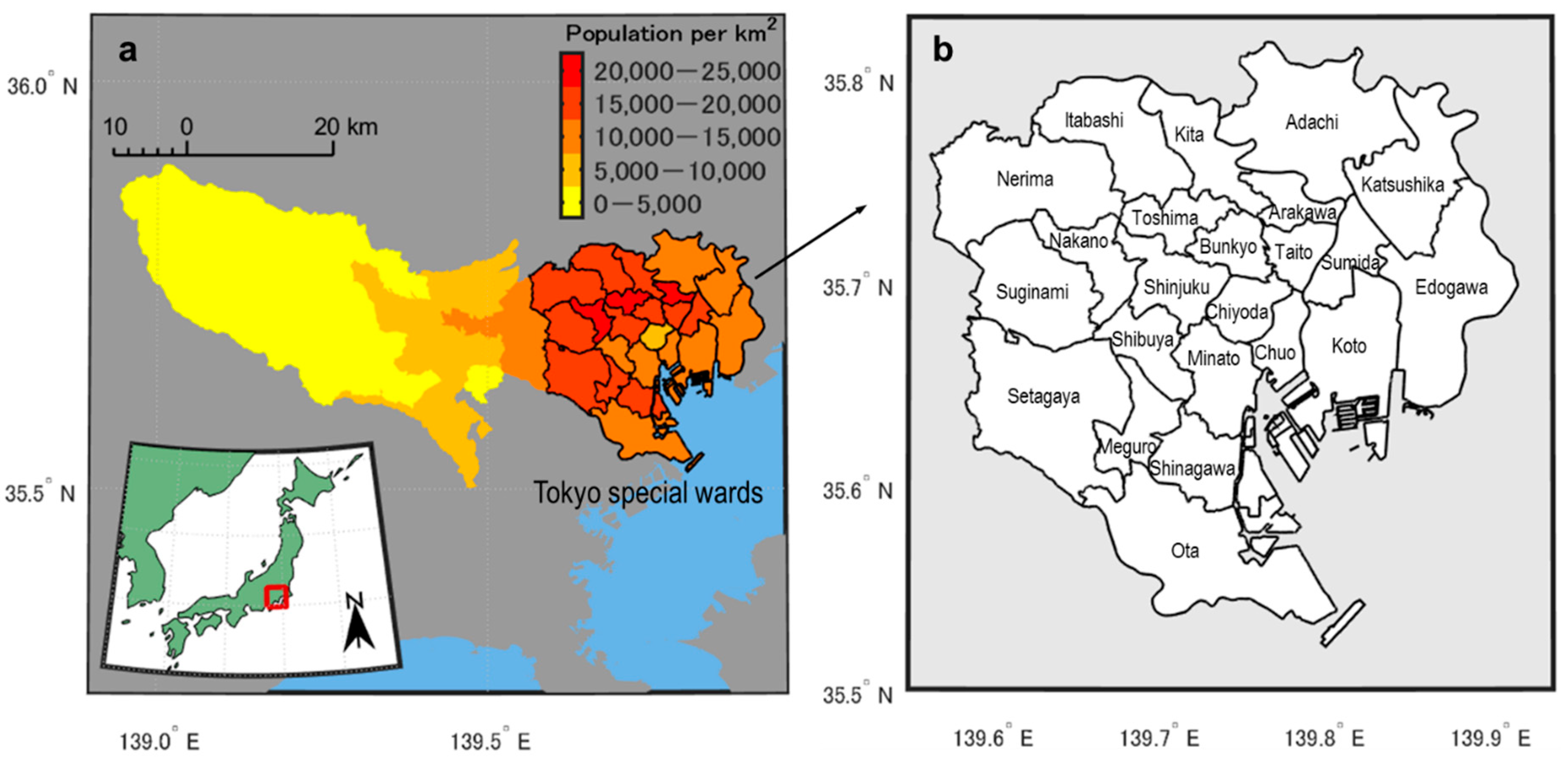
2.1. Study Area

The study area covers the entire urban area of Tokyo metropolis, the capital of Japan. This area, named the special wards, houses conterminous 23 municipalities (wards) that together make up the core and the most populous single city of Tokyo metropolis, and also of Japan (Figure 1). The population is approximately 9.3 million people in an area of 625 km2 according to the 2015 National Population Census [13]. Each of the 23 municipalities has an average area of 27.2 km2 (range: 10.1–58.0 km2). The topography is fairly flat. The area experiences a humid subtropical climate, with the mean annual temperature of 15 °C and the mean annual precipitation of 1500 mm yr−1 [13]. Land cover comprises various types of anthropogenic features (e.g., asphalt, concrete, and roof materials) intersecting with the semi-natural environment (e.g., trees, grass, soil, and water). Trees are mainly located within the parks, residential areas, and along the streets, thereby representing a typical distribution of trees in an urban area.

2.2. WordView-2 and WorldView-3 (WorldView-2/3) Datasets

Cloud-free WorldView-2/3 images (DigitalGlobe, Inc., Westminster, CO, USA) acquired during different tree phenology periods were used in this study (Table 1). In Tokyo, April to September are considered spring and summer months belonging to the “leaf-on season” when most trees develop a green canopy, while October to March are autumn and winter months belonging to the “leaf-off season” when the leaves of deciduous trees begin changing color and falling. As the image acquisition dates were selected based on the data availability and cloudless sky conditions over the site, one pair of images for both leaf-on and leaf-off seasons were not available for the same year.
We used the WorldView-2/3 datasets of eight multispectral bands with 2 m ground sample distance, including Coastal (Band 1; 400–450 nm), Blue (Band 2; 450–510 nm), Green (Band 3; 510–580 nm), Yellow (Band 4; 585–625), Red (Band 5; 630–690 nm), Red Edge (Band 6; 705–745), NIR1 (Band 7; 770–895 nm), and NIR2 (Band 8; 860–1040 nm). The satellite has a swath width of 13.1 km. We obtained the WorldView-2/3 satellite imagery for the entire study area by merging the sets of cloudless images for each season (Figure 2a,b).
The WorldView-2/3 images were subjected to atmospheric and geometric corrections before processing and classification. Each multispectral digital number image was converted to Top of Atmosphere (TOA) radiance based on the radiometric calibration parameters and the standard correlation formula [14,15]. For each band, surface reflectance was generated based on the sensor response function and specific atmospheric conditions. The datasets were orthorectified and projected to the WGS-84 UTM Zone 54N system.

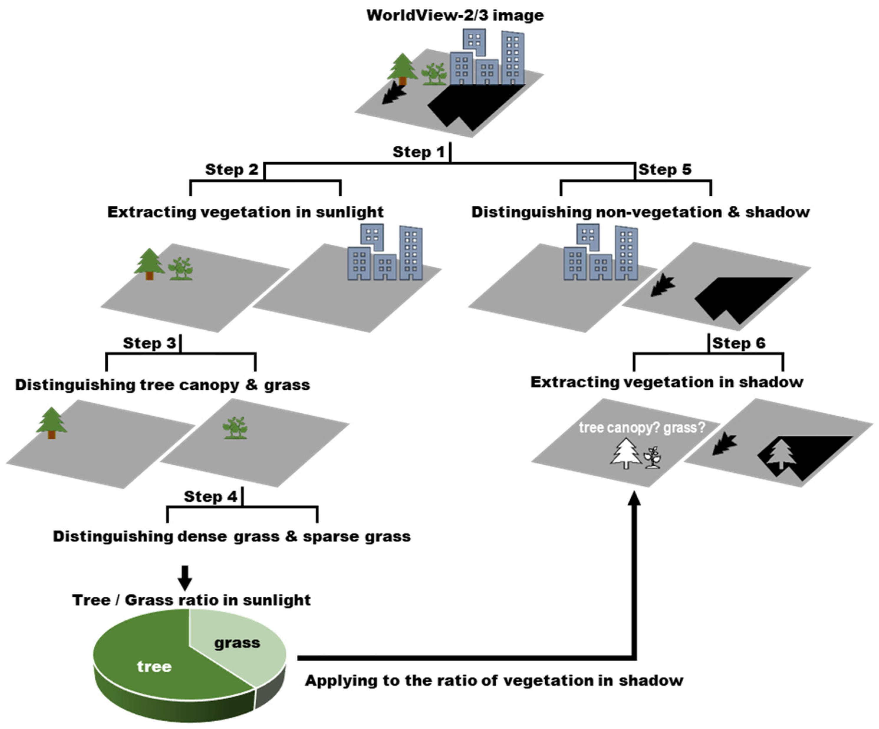
2.3. Tree Canopy Extraction from Background

After merging the WorldView-2/3 images and performing radiometric calibration, we separated the land cover into categories. A multiple stepwise masking procedure using the bi-modal histogram threshold method was employed to extract the tree crowns from the remaining background [16]. Figure 3 illustrates the segmentation procedure that consists of six steps. Here, a pixel-based classification was performed [17].
First, we selected the training sample pixels from 12 categories: eight non-vegetation (soil, sand, asphalt/concrete, high-rise building, low-rise building, water, shaded non-vegetation, and high Normalized Difference Vegetation Index (NDVI) non-vegetation), and four vegetation (tree canopy, dense grass, sparse grass, and shaded vegetation) categories. More than 1500 training samples per image were chosen almost equally for each land category, fulfilling the accuracy requirement of the decision tree methods for land cover classification [18]. Training samples were randomly selected in the study area to avoid spatial bias.
After the training samples were obtained, we used the normalized difference index ( N D I = ( B a n d   A B a n d   B ) / ( B a n d   A + B a n d B ) ) as a classifier to distinguish each pixel into different land categories. Bands A and B are, respectively, the reflectance data of the WorldView-2/3 spectral bands. We produced a pixel number histogram of the NDI values calculated from two different land categories. All 64 possible band combinations of the eight spectral WorldView-2/3 bands were tested to determine an appropriate band from the two sets (Bands A and B) for obtaining a bi-modal (two-peak) NDI histogram. Subsequently, a splitting variable (threshold) around the bottommost point (valley) of the bi-modal NDI histogram was determined manually by visual inspection. The NDI values of 64 different band combinations were tested at each classification step, and the classification performance was optimized by trial-and-error. Tree canopy land cover map was produced based on the best result.
Since we were not successful at distinguishing the vegetation type in the shaded area, we calculated the total area of the shaded tree canopy cover using the ratios of the vegetation categories as follows: T s h a d o w = V s h a d o w × ( T s u n l i t / V s u n l i t ) , where Tshadow and Tsunlit are the percent tree canopy cover (%) in shadow and sunlit areas, respectively; Vshadow and Vsunlit are the percent vegetation cover (%) in shadow and sunlit areas, respectively. We assumed that the ratios of the vegetation categories in shadow and sunlit areas are approximately the same in a large area.

2.4. Reference Data of Tree Canopy Cover

Vegetation maps obtained from the field surveys and aerial photographs were used as a reference to test the accuracy of the output of our WorldView-2/3 image classification analysis.

2.4.1. Field Investigation

We surveyed the vegetation cover in an urban park of 0.3 km2, which is located in Koto-ward in December 2016 (Figure 2, B3). Hardcopies of the WordView-2 images acquired in both the leaf-on and leaf-off seasons were brought to the field to locate the tree crown and also to confirm the tree types. We classified the trees with height >2 m as “tall” and <2 m as “small.” We manually outlined the vegetation in the WordView-2 image and created a 2D polygon map of eight vegetation types (six tree types and dense/sparse grass). The image analysis was conducted using ArcGIS (Ver. 10.3.1; Environmental Systems Research Institute, Inc., Redlands, CA, USA).

2.4.2. Aerial Photograph Interpretation

We used one scene of the true color GEOSPACE digital aerial photographs with 0.25 m spatial resolution acquired in March 2013. The photograph covered 3.0 km2 of a dense urban setting with many high-rise buildings around the Tokyo metropolitan government office in Shinjuku-ward (Figure 2, B2). We manually created 2D polygons of each vegetation land cover category (tree canopy, grass, and shaded vegetation) in the aerial photograph by visual inspection using ArcGIS.

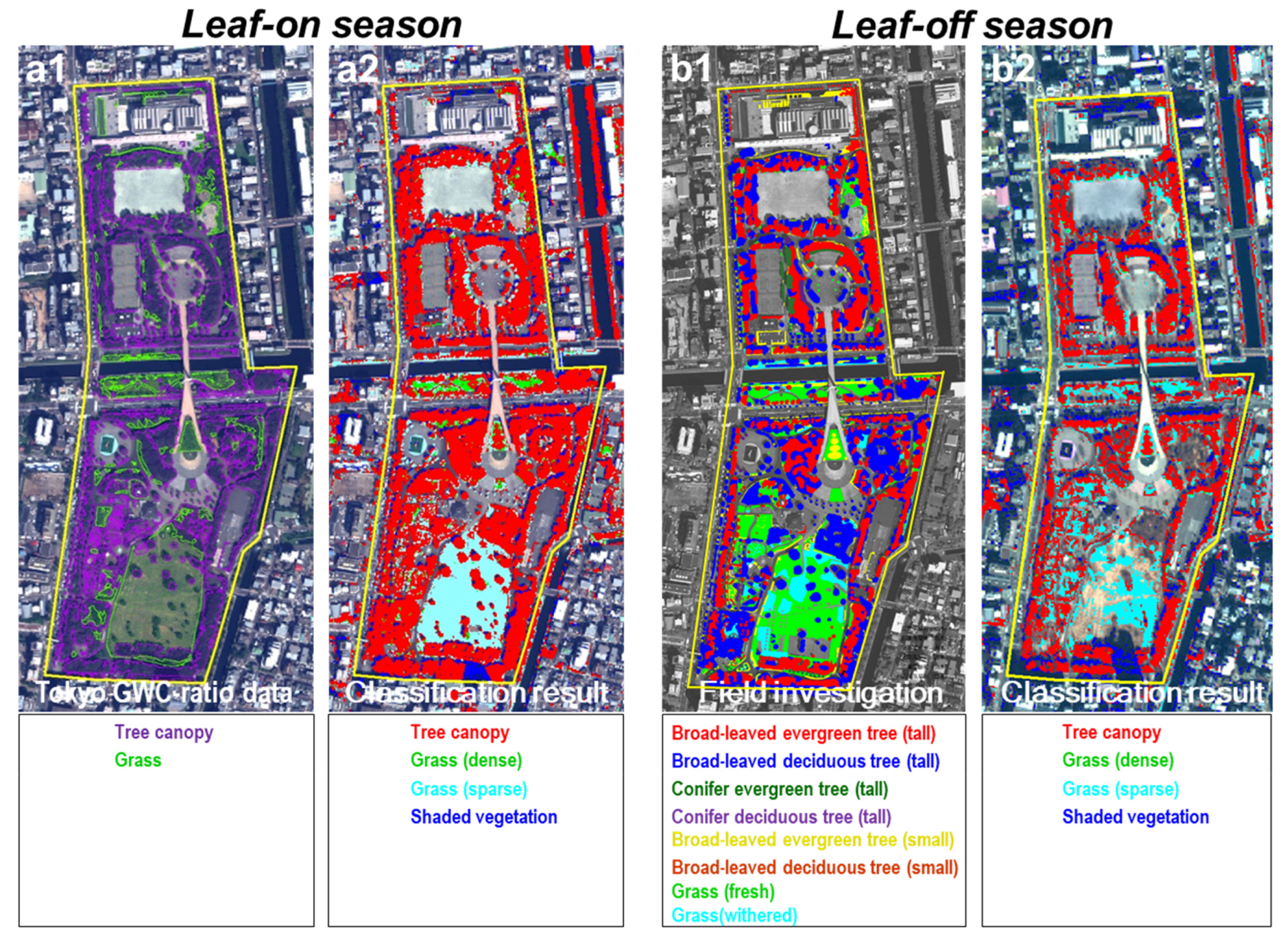
2.4.3. Tokyo Green and Water Coverage Ratios (Tokyo GWC-Ratio Data) Based on Aerial Photograph Interpretation

The green and water coverage ratios in Tokyo special wards (our study area) have been surveyed every five years since 2003 by the Tokyo metropolitan government. This data (called Tokyo GWC-ratio data hereafter) were created to calculate and monitor the ratio of the total area of parks, water surfaces, and ground surfaces covered by greenery in the entire region. The land cover map of tree canopy and grass were surveyed in the leaf-on season. We used the 2013 data to assess the accuracy of our image classification results obtained for the leaf-on season only.
The method adopted to analyze the green coverage data is based on the extraction of features of interest (tree canopy and grass) from aerial photographs by visual inspection. The aerial photographs covered all Tokyo special wards (approx. 625 km2) with the ground resolution of no less than 0.2 m. The photographs for the 2013 data (and also 2018 data) were taken in November of the preceding year for both datasets. Tree canopy and grass areas were delineated by visual inspection by enlarging the photographs to a scale of 1:1000 so that a 1 m2 object on the ground could be visible in a 1 mm2 area on the computer screen. Therefore, every single tree and a patch of grass larger than 1 m2 were delineated. The areas of tree and grass were digitized as a polygon layer and saved as a shape file in ArcGIS. In case the ground object was difficult to identify due to some cloud and shadow interruptions, the analyst conducted an on-site visit for confirmation. Cultivated areas of farmlands, and algae and weed in rivers and lakes were excluded.
The shape of the tree canopy in streets and parks is relatively constant due to the forest management by local authorities. According to the Tokyo GWC-ratio data, there is only a small difference (−0.2%) between the 2013 to 2018 data on the ratio of tree canopy coverage in the special wards. Thus, it is likely that no significant tree canopy size and leaf area changes can occur from the date of the satellite imagery data (between 2013 and 2017) to the date of the reference data (December 2016 for the field investigation, March 2013 for the aerial photograph interpretation, and November 2012 for the 2013 Tokyo GWC-ratio data). This was also proved in the field survey and aerial photographs; trees were mostly identified at the same position as in the WordView-2/3 images with similar crown sizes.

2.5. Approximate Model for the Relationship between Leaf Area Index (LAI)–Vegetation Indices (VI)

To infer LAI from the WordView-2/3 imagery, we developed an approximate model to evaluate the relationship between the vegetation index (VI) and in situ leaf area index (LAI; m2 m−2) measurement data. Then, this model was used to calculate the pixel-based tree canopy LAI from the corresponding VI data. The LAI is the total one-sided leaf area per unit ground surface [19].
Several studies have developed LAI prediction models using vegetation indices (VI) for a variety of vegetation cover, including grasslands and trees [20,21]. The NDVI = ( ( N I R r e d ) / ( N I R + r e d ) ), which is the most widely used VI, quantifies the response of the vegetation to near-infrared reflectance (NIR) and red absorption [22,23]. The red and NIR of the WordView-2/3 data correspond to spectral bands Band 5 and Band 7, respectively. The NDVI is recognized as the most stable vegetation index for estimating the LAI [24,25], yet the methodological limitation of the VI and notably the NDVI were shown by Pinty et al. [26]. Thus, in this study, four different additional vegetation indices, which have also been widely applied in the literature to derive LAI, were examined (Table 2). The red edge of the WordView-2/3 data correspond to spectral band, Band 6. The VI obtained with different extraction methods was tested to evaluate the relationship between the VI and LAI measurement data. We tested two VI-extraction window sizes (1, 3 × 3) close to the LAI measurement point, i.e., a VI value acquired from (1), which is the closest pixel to the LAI measurement point, and (2) a block of nine (3 × 3) pixels constituted with the closest pixel to the LAI measurement point at the center and its surrounding eight pixels. For the 3 × 3 extraction window, we tested two values of each VI (mean and maximum) for comparison with the LAI data at the center of those nine pixels.
The LAI–VI approximate model was then developed for both the leaf-on and leaf-off seasons. We optimized the model parameters to achieve 1:1 ratio between the estimated LAI and the observed LAI to avoid overestimation.

2.6. In Situ Tree LAI Measurement

We measured the tree canopy LAI (m2 m−2) for Ginkgo biloba, Cornus florida, Prunus spp., Acer buergerianum, Zelkova serrata, Platanus spp., Cinnamomum camphora, Lithocarpus edulis, Morella rubra, Magnolia kobus as these are the 10 species most commonly planted in Tokyo special wards. Several other species found in the field were also measured. The LAI data was collected from evergreen and deciduous trees for the leaf-on season, and from evergreen trees for the leaf-off season. A LAI-2200 plant canopy analyzer (LI-COR Biosciences Inc., Lincoln, NE, USA) was used for the tree canopy LAI measurement in the field (Supplementary Material Figure S1). LAI measurement points were deployed over three areas in Figure 2 (A1 and B1, A2 and B2, A3 and B3) for the leaf-on and leaf-off seasons, respectively. The exact location of the LAI measurement points was recorded by GPS to allow subsequent extraction of the nearby VI value from satellite images. A field survey was conducted in each area in 2018, in the same month when the satellite image of each respective area was photographed. A total of 386 and 268 tree canopy LAI data points were collected in the leaf-on and leaf-off seasons, respectively.
All the LAI measurements were conducted on either cloudy days, soon after the sunrise, or soon before the sunset, to avoid measurement errors, which may be caused by direct sunlight [31]. Moreover, the operator always stood between the sensor and the sun to conduct measurements under the same light conditions to reduce measurement bias. To shield the hemispherical sensor of the plant canopy analyzer from the operator and any objects except trees, we only used the data obtained within a front azimuth angle between 0° and 30° and a vertical zenith angle between 0° and 43° in accordance with the procedure suggested by Dufrêne and Bréda [32]. Each LAI data point represents an average of five measurements taken under a single tree canopy, and additional one measurement of above-canopy radiation taken in the nearby open space as a reference. Incidentally, it is likely that the in situ LAI data include some contribution of woody elements, so-called plant area index, rather than an actual leaf area index [7]. Thus, we measured the LAI of leafless trees (i.e., the woody element only) in winter to evaluate the degree of overestimation in the LAI data obtained by the plant canopy analyzer.
All the statistical analyses in this study were performed using MATLAB (Ver. 2018b, The MathWorks, Inc., Natick, MA, USA) and BullCurve for Excel (Ver. 3.4.3, Social Survey Research Information Co., Ltd., Tokyo, Japan).

2.7. LAI Estimates Using Landsat5-TM and Landsat8 Satellite Data

We also estimated the tree canopy leaf area using Landsat5-TM and Landsat8 imagery (30 m resolution). For this purpose, we adopted a previously reported LAI−NDVI relationship: L A I = 0.419 e N D V I / 0.270 for Landsat5-TM imagery derived from a broad-leaved forest area in Japan [33], and L A I = 3.440 e N D V I 3.380 for Landsat8 imagery derived from an urban park tree canopy in South Korea [34]. Landsat5-TM imagery was acquired on 11 October, 2010, and Landsat8 imagery was acquired on 27 October, 2016. The season of image acquisition was chosen to coincide with the WorldView-2 imagery, which was acquired on 27 October 2016, for a more accurate comparison. Cloudless images were selected. The Landsat scenes were obtained from the United States Geological Survey (USGS) Earth Explorer website (https://earthexplorer.usgs.gov/). The multispectral digital numbers were converted using the conversion coefficients provided by the Landsat metafiles to obtain Top of Atmosphere (TOA) spectral reflectance. Band 4 (Red) and Band 5 (NIR) of the Landsat scene were used to calculate the NDVI for the LAI estimates.

3. Results

3.1. Determination of Masking Thresholds and Band Combinations for Tree Canopy Extraction

In total, five land cover classes (tree, grass, shaded vegetation, non-vegetation, and shadow/water) were produced following the stepwise masking approach and determining the ideal NDI band combinations and thresholds (see Section 2.3). Table 3 shows the optimized two-band combinations for obtaining the bi-modal NDI histogram and thresholds for each classification step. The bi-modal NDI histograms obtained for each satellite imagery is shown in the Supplementary Material section in Figure S2 for the leaf-on season, and Figure S3 for the leaf-off season. First, the land surface was separated with the NDI calculated from Band 5/Band 7, namely NDVI. In areas with a high NDVI, some pixels were non-vegetation pixels. Thus, in the second step, those non-vegetation pixels in the high NDVI areas were excluded using the NDI calculated from Band 5/Band 6. In the third step, the NDI calculated from Band 1/Band 3 clearly separated the tree canopy and grass, using the same threshold value (0.2) for both the leaf-on and leaf-off seasons. In the fourth step, the dense grass and sparse grass was separated. In the fifth and sixth steps, the vegetation was extracted from the area of low NDVI pixels that was obtained in the first step. Here, to distinguish the vegetation and non-vegetation in the shadow area, the threshold value was a key factor that strongly affected the classification accuracy. Hence, we manually determined an optimum threshold value for each satellite image that produced the best classification result for extracting vegetation data in the shadow area. We were not successful in distinguishing the types of vegetation (tree canopy and grass) in the shadow area because of the weak spectral capability.

3.2. Accuracy Assessment

Figure 4 and Figure 5 present the resultant classification maps of vegetation (tree, grass, and shaded vegetation) using the pixel-base classification method in the leaf-on and leaf-off seasons, respectively. The mapping results we obtained from WordView-2/3 (Figure 4(a3,b3), and Figure 5(a2,b2)), agree with the vegetation maps generated from aerial photographs (Figure 4(a2,b2), and Figure 5(a1)), and field investigations (Figure 5(b1)). The overall difference of the tree canopy cover was less than 5.5% (Table 4). However, those two sites show only a small area and do not therefore fully represent the land cover in the entire study area. Thus, we made a comparison across municipalities for a comprehensive accuracy assessment. The tree canopy cover was found to be in good agreement with the Tokyo GWC-ratio data showing ±5% difference overall and 1.2% difference for the entire Tokyo special-ward area (Supplementary Table S1). Figure 6 shows a summary of the overall classification accuracy. The classification result achieved nearly 1:1 ratio against the validation data from field investigation and aerial photograph interpretation. Thus, the classification accuracy was nearly equal in the study area and sufficient for a comprehensive assessment of the tree canopy cover with a margin of difference of 5.5% at 3.0 km2 small district level, 5.0% at 60.9 km2 municipality level, and 1.2% at 625 km2 city level (Supplementary Table S1), compared to aerial photograph interpretation.

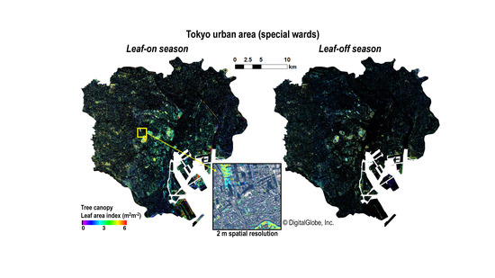
3.3. Tree Canopy LAI Mapping from VI

The measured LAI from the three sites ranged between 1.9 and 10.7 m2 m−2 (N = 386, mean ± SD = 5.4 ± 2.0) for the leaf-on season and between 1.8 and 9.7 m2 m−2 (N = 268, mean ± SD = 4.6 ± 1.3) for the leaf-off season, respectively. The LAI data followed a normal distribution for both the leaf-on season (χ2 = 23.6, 2 df, p < 0.001) and the leaf-off season (χ2 = 18.1, 2 df, p < 0.001). Among the four VI extraction methods examined herein (Section 2.5), the maximum VI selected within a block of nine pixels (3 × 3) showed the highest correlation with the LAI data (Supplementary Material Figure S4, a11–a15 for the leaf-on season, and b11–b15 for the leaf-off season). The Red Edge NDVI (RE−NDVI) was not correlated with LAI. The relationship between the maximum VI (except RE−NDVI) and the observed LAI data was equal during the leaf-on seasons (Spearman’s rank correlation coefficient, R = 0.44), yet the NDVI showed a slightly better relationship during the leaf-off season (Spearman’s rank correlation coefficient, R = 0.34 for NDVI, and R = 0.30 for WDRVI and EVI2).
As an example of the LAI−VI relationship, Figure 7 (a1 and b1) shows the relationship between the maximum NDVI and the observed LAI data for each tree species. The LAI values converge to the value of 2 when the NDVI values decrease. This result agrees with our observation for the leafless trees during the leaf-off season that showed an LAI value of 1.8 ± 0.4 m2 m−2 (mean ± SD, N = 39). Thus, the LAI estimates derived using the plant canopy analyzer include an overestimation of 1.8 m2 m−2 caused by the misdetection of the woody elements (i.e., tree trunk and branches) as leaves. Accordingly, we subtracted this overestimation from the observed LAI data and obtained the LAI−NDVI approximate model for the leaf-on season ( L A I = 0.1 e N D V I / 0.179 ) and the leaf-off season ( L A I = 0.1 e N D V I / 0.188 ) (Figure 7, a1 and b1). The LAI was saturated at an NDVI of 0.8 for both the seasons, and thus, the applicability of these models was uncertain at an NDVI > 0.8. Hence, we replaced the NDVI values > 0.8 with 0.8 to estimate the LAI. The same was true for the other VI, where the VI values appeared to saturate at −0.15 for the WDRVI1, 0.2 for the WDRVI2, and 1.6 for the EVI2, respectively (see Supplementary Material Figure S4, a11–a15 for the leaf-on season, and b11–15 for the leaf-off season). Therefore, the maximum VI value for each LAI−VI model was set to that respective saturation VI value (Supplementary Material Table S2).
Figure 7 (a2,b2) shows the observed LAI data in association with the estimated LAI using the LAI−NDVI approximate model as an example of the accuracy achieved from the LAI−VI model. The 1:1 ratio between the observed and estimated LAI is an expected outcome because the LAI−NDVI approximate model was adjusted manually to obtain this result (for detail see Section 2.5). Even some plots in Figure 7(a2,b2) were out of the 95% prediction interval, large errors were not caused by a particular tree species. Similarly, there was no significant difference between the estimated LAI and observed LAI for most tree species (Figure 7c). The root-mean-square errors (RMSEs) for the estimated LAI for leaf-on/leaf-off seasons were 2.11/2.41, 2.54/2.30, 2.35/1.93, and 2.34/1.86 for LAI−NDVI, LAI−WDRVI1, LAI−WDRVI2, and LAI−EVI1, respectively (Supplementary Material Table S2).
Figure 8b presents an example of the LAI map generated using the LAI−NDVI approximate model. Here, we calculated LAI in pixel i by sequentially executing the following code through all the pixels defined as tree canopy using the image classification:
L A I ( i ) = A * e ( m a x V I ( i ) / B )
where, A and B are the specific coefficients for each LAI−VI model as shown in Supplementary Material Table S2. The maxVI (i) value is the maximum VI within a block of nine pixels with pixel i at the center. As a result, the estimated total leaf area in Tokyo special wards in the leaf-on season was twice that in the leaf-off season. Table 5 presents the summary of the estimated results for the entire area and the subarea illustrated in Figure 8 with the dense tree canopy covering most of the ground. For both areas, the total leaf area for the WorldView-2/3 results was higher than the Landsat5-TM and Landsat8 results. The same was true for the entire Tokyo special-ward area: the total leaf area estimated from WorldView-2/3 was 1.9–6.2 times higher than the Landsat5-TM and Landsat8 results (Table 5).

4. Discussion

In this study, we aimed to develop a method to identify the small patches of individual trees in a highly urbanized landscape at the mega-city scale, which is seldom studied. We selected the entire urban area of Tokyo (special wards consisting of 23 municipalities) as the study area and utilized the high-resolution WorldView-2/3 satellite imagery to map and estimate the leaf area of the tree canopies. Land coverage of trees by pixel-based image classification was estimated with less than 5.5% difference from the test areas where the field surveys and aerial photograph interpretation were performed. At the municipality scale, the tree canopy cover was estimated with ± 5% difference from the Tokyo GWC-ratio data derived from the aerial photograph interpretation.
Once the tree canopy was identified, we developed a simple method to estimate their leaf area. The results revealed a relationship between the in situ LAI measurement data and the three VI data (NDVI, WDRVI, and EVI2, except the RE−NDVI) from the WorldView-2/3 imagery. The maximum VI selected within a block of nine pixels (3 × 3) was the only one to produce a significant relationship with the LAI data. The others (a VI value at the nearest pixel to the LAI measurement point and the average VI of the nine-pixel (3 × 3) window with the LAI measurement point at the center pixel) were not correlated with the LAI (see Supplementary Material Figure S4). The major reason for their weak LAI−VI relationships can be the effect of geolocation uncertainties in the satellite images and the uneven illumination on the tree crown caused by the shaded and unshaded areas. The rounded shape of an individual tree crown may cause variations in canopy illumination. These variations can be detected in high spatial resolution satellite imagery (2 × 2 m) and may have a significant influence on spectral reflectance. Shadows have lower reflectance intensity than unshaded areas and can cause the VI values to become lower than their actual values. Hence, if the shaded area is included within a block of 3 × 3 pixels, an average VI value for the window of nine pixels will be unreasonably low. This can lead to the weak LAI−VI relationships. However, using the maximum VI value within a block of 3 × 3 pixels means that the VI at the center of the nine pixels is more likely to be chosen from the unshaded area of the tree crown and, thus, it becomes less affected by the uneven illumination effect. Hence, we used the LAI−VI relationship based on the maximum VI to calculate the LAI.
We investigated the LAI−VI relationships in two seasons (leaf-on and leaf-off seasons) because there was a possibility that these relationships are not uniform over the year and might fluctuate seasonally with the phenological stages of the vegetation [35,36]. In fact, Qiao et al. [25] used the NDVI from MODIS satellite imagery and found significant LAI−NDVI relationships during the vegetation’s growing and declining periods, whereas a poor relationship was observed during the flourishing period. We focused only on the two phenophases, namely the vegetation non-active period during January–February (except one satellite imagery acquired on April 4) and the vegetation active period during September–November (corresponding approximately to the “declining period” [25]), and thus, the other phenological transition stages such as periods of growing and flourishing were neglected in this study. This might be the reason why the LAI−VI relationships in our results were not visibly affected by the phenology because the flourishing period (the most uncertain period for the LAI−VI relationships) was not considered. Additional work is warranted to evaluate more cases in different seasons for a comprehensive and more accurate assessment.
Using the obtained LAI−VI approximate model, we estimated the tree leaf area over Tokyo’s 23 special wards and also for the area shown in Figure 8 that can be characterized as a typical urban environment with the built-up area including parks and tree-lined streets. The obtained leaf area from the WorldView-2/3 imagery was higher than the results suggested in [33,34] (Table 5). The problem with the lower NDVI values arising from mixed pixels (i.e., a pixel that encompasses vegetation with different physical properties) was previously documented [37]. Given the relatively larger pixel size of the Landsat imagery (30 × 30 m) compared to the WorldView-2/3 imagery (2 × 2 m), the mixed pixel effect was strong in the highly heterogeneous urban environment and thus lowered the VI and the LAI values accordingly. In fact, the LAI−NDVI relationships proposed by Hoshi et al. [33] and Kimm et al. [34] were targeted for broad-leaved trees with continuous canopy, and thus, their applicability to estimate the leaf area in a highly urbanized landscape with small patches of individual trees was uncertain. On the contrary, for the same reason, the gap between the results was smaller for the estimates in the dense tree canopy region (Table 5).
This study only focused on extracting the tree canopy cover and did not consider the differences in species and vegetation types in the shadow area. In addition, the problem of saturation of VI at high LAI also needs to be addressed (notably the NDVI in Figure 7 a1 and b1, and for the other VI see Supplementary Material Figure S4). The VI data are derived from the two-dimensional picture, and therefore, the VI, notably the NDVI, is known to be less sensitive to high LAI values when the vegetation is dense [21,24,38]. Thus, the use of VI poses a challenge because the leaf area of an overlapping canopy and a tall tree is difficult to quantify accurately using the LAI−VI relationship. There is a need for robust algorithms to fully evaluate the leaf area in the pixels with high VI values. Although NDVI is one of the most reliable index for estimating LAI [24,39,40], some other vegetation indices tested in this study (RE−NDVI, WDRVI, and EVI2) are also proposed with their own advantages. Several new vegetation indices such as the near-infrared reflectance of vegetation (NIRv) [41] are reported to possess sufficient sensitivity in high-density vegetation areas. Another uncertainty in the LAI−VI relationship is the effect of understory vegetation. During the LAI measurement, the view angle was skywards; thus, the vegetation below the sensor (≈1.5 m high in this study) was not recorded and, therefore, excluded from the ground truth. In a closed dense canopy, the influence of understory vegetation can be neglected, but in a sparse canopy, understory vegetation can influence the VI value, which is observed from the sky above [42,43]. In fact, a recent study showed that the relationship between the LAI and several vegetation indices (including NDVI) improved substantially when the observation points with understory vegetation were excluded [44]. The extent of the effect of understory vegetation on this study’s findings should be addressed in a future study to provide more accurate and consistent LAI estimates.
Our future work will focus on the unsolved issues to produce a more complete leaf area inventory for the Tokyo urban area. Using multi-temporal data is known to offer a promising increase in the success rate of mapping urban trees and/or species composition [12,45]. As the WorldView-2/3 satellite can provide images with near-daily revisit times, future research will also include the evaluation of the multi-temporal datasets to improve estimation accuracy by mitigating the uncertainties in the seasonal variations in the LAI−VI relationship caused by the differences in phenology and species type.

5. Conclusions

To the best of our knowledge, only a few studies have conducted the accuracy assessment of tree canopy cover maps derived from high-resolution (2 m) satellite imagery in mega cities. Our results can be summarized as follows:
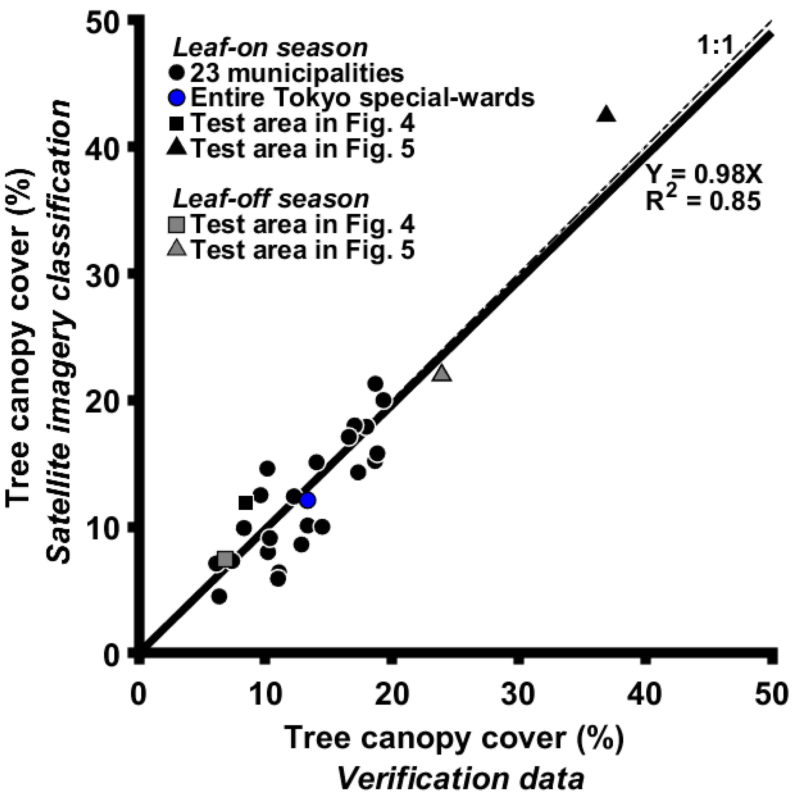
  • The WorldView-2/3 imagery has the ability to map tree canopy cover in a highly heterogenic urban environment with acceptable accuracy. The error margin of the tree canopy cover can reach 5.5% at the 3.0 km2 small district level, 5.0% at the 60.9 km2 municipality level, and 1.2% at the 625 km2 city level, compared to the values based on aerial photograph interpretation.
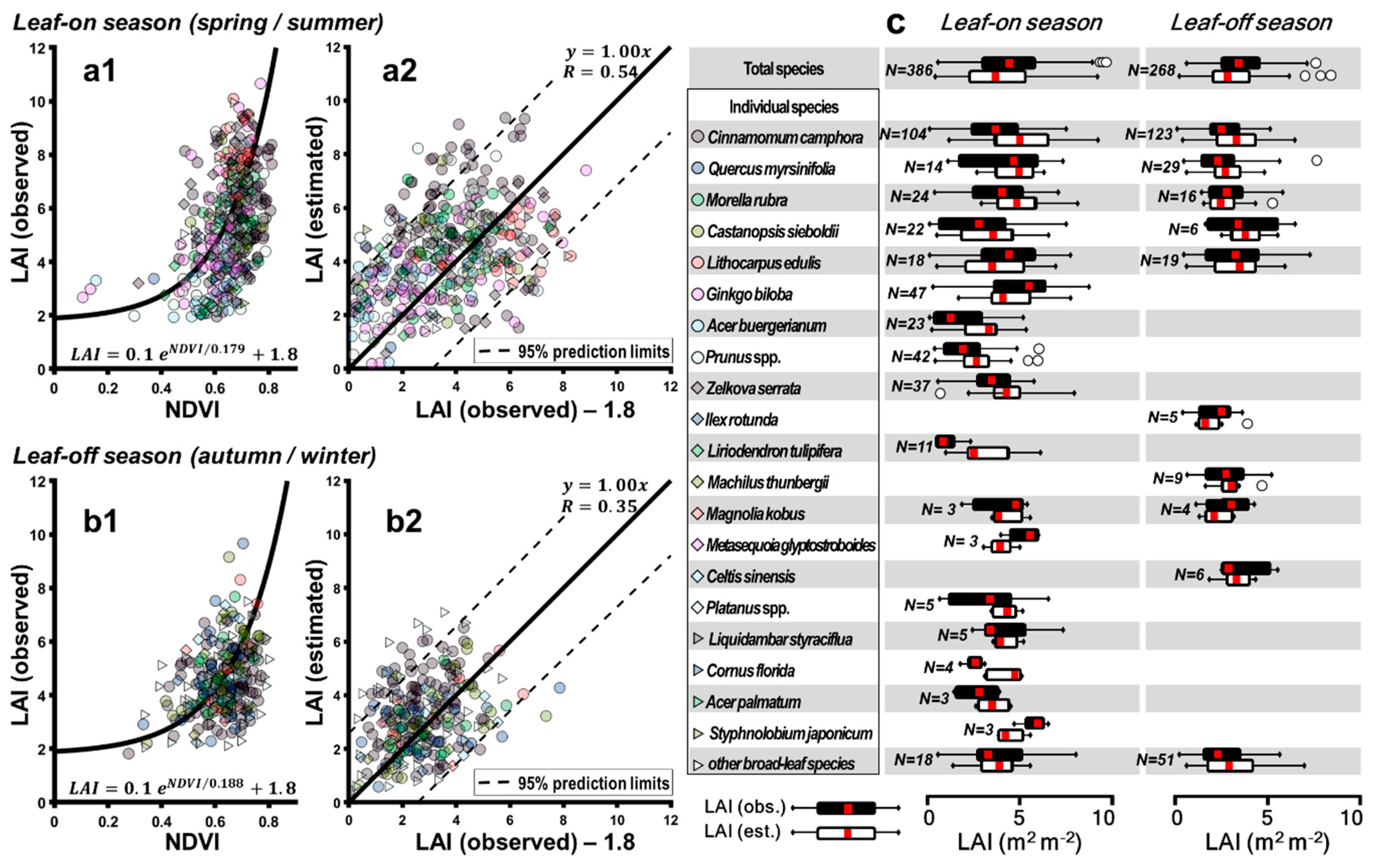
  • LAI was estimated with acceptable accuracy for the leaf-on season (September–November, corresponding to a vegetation declining period in autumn) and the leaf-off season (January–February, corresponding to a vegetation non-active period in winter) using the LAI−VI relationships.
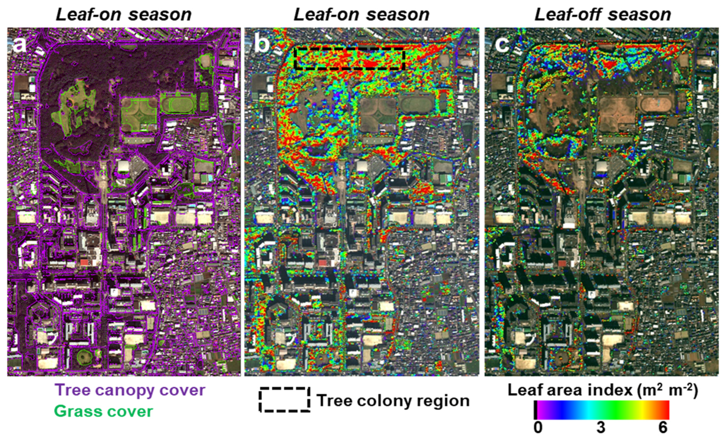
  • The estimated LAI and the total leaf area in Tokyo urban area was 1.9–6.2 times higher than the results from the Landsat5-TM and Landsat8 images using the LAI−NDVI relationships reported in a previous study.
Timely and accurate acquisition of the information on the status and structural changes in urban forests is crucial to develop strategies for sustainable city development and air quality improvement. The method developed in this study offers a practical solution to estimate the tree leaf area in megacity-scale regions in different tree phenology seasons. Maps of the leaf area at the individual tree scale can improve the understanding of the effect of the ecosystem services/disservices on urban systems, and enhance the efficiency of green infrastructure investment and implementation.

Supplementary Materials

The following are available online at https://0-www-mdpi-com.brum.beds.ac.uk/2072-4292/12/9/1505/s1, Table S1: Comparison of the vegetation land cover for each 23 municipalities in Tokyo special wards estimated by aerial photograph interpretation (Tokyo GWC-ratio data), and WorldView-2/3 imagery classification (this study). Figure S1: LAI measurement using LAI-2200, Plant Canopy Analyzer. Measurements were made below the tree canopy at the breast height with the sensor facing upward. Figure S2: Bi-modal histograms used to obtain the threshold values for image classification (leaf-on season). The histograms are normalized with the total number of each classification category for each satellite imagery. Figure S3: Bi-modal histograms used to obtain the threshold values for image classification (leaf-on season). The histograms are normalized with the total number of each classification category for each satellite imagery. Figure S4: Relationships between the VI and the observed/estimated LAI for the leaf-on season (upper panels: a) and the leaf-off season (lower panels: b). Columns (15), (610), and (1115) are the relationship between the VI obtained with different extraction methods and the observed LAI, respectively. The blue line in columns 11, 13, 14, 15 represents LAI–VI approximate model derived from the maximum VI and observed LAI data. Columns 16, 17, 18, and 19 are performances of the LAI–VI approximate model developed herein. The y = 1.0x line is fitted. Table S2: The obtained LAI–VI approximate models.

Author Contributions

Conceptualization, Y.K.; methodology, Y.K. and S.H.; software, Y.K. and S.H.; validation, Y.K. and S.H.; formal analysis, Y.K. and S.H.; investigation, Y.K. and S.H.; resources, Y.K. and S.H.; data curation, Y.K. and S.H.; writing—original draft preparation, Y.K.; writing—review and editing, S.H. and A.T.; visualization, Y.K. and S.H.; supervision, Y.K. and A.T.; project administration, Y.K.; funding acquisition, Y.K. All authors have read and agreed to the published version of the manuscript.

Funding

This research was funded by the Tokyo Metropolitan Government Bureau of Environment, and Grant-in-Aid for Scientific Research, No. 19K12302 (C) from the Japan Society for the Promotion of Science.

Acknowledgments

We are grateful to the Tokyo Metropolitan Government Bureau of Environment that provided the Tokyo GWC-ratio data. We also would like to thank Kazukiyo Takahashi of the Tokyo Metropolitan Research Institute for Environmental Protection who helped with the collection of the LAI data.

Conflicts of Interest

The authors declare no conflicts of interest.

References

  1. Grote, R.; Samson, R.; Alonso, R.; Amorim, J.H.; Cariñanos, P.; Churkina, G.; Fares, S.; Le Thiec, D.; Niinemets, Ü.; Mikkelsen, T.N.; et al. Functional traits of urban trees: Air pollution mitigation potential. Front. Ecol. Environ. 2016, 14, 543–550. [Google Scholar] [CrossRef]
  2. Endreny, T.A. Strategically growing the urban forest will improve our world. Nat. Commun. 2018, 9, 1160. [Google Scholar] [CrossRef] [PubMed] [Green Version]
  3. Roeland, S.; Moretti, M.; Amorim, J.H.; Branquinho, C.; Fares, S.; Morelli, F.; Niinemets, Ü.; Paoletti, E.; Pinho, P.; Sgrigna, G.; et al. Towards an integrative approach to evaluate the environmental ecosystem services provided by urban forest. J. For. Res. 2019, 30, 1981–1996. [Google Scholar] [CrossRef] [Green Version]
  4. Shrivastava, M.; Andreae, M.O.; Artaxo, P.; Barbosa, H.M.J.; Berg, L.K.; Brito, J.; Ching, J.; Easter, R.C.; Fan, J.; Fast, J.D.; et al. Urban pollution greatly enhances formation of natural aerosols over the Amazon rainforest. Nat. Commun. 2019. [Google Scholar] [CrossRef] [PubMed] [Green Version]
  5. Eisenman, T.S.; Churkina, G.; Jariwala, S.P.; Kumar, P.; Lovasi, G.S.; Pataki, D.E.; Weinberger, K.R.; Whitlow, T.H. Urban trees, air quality, and asthma: An interdisciplinary review. Landsc. Urban Plan. 2019, 187, 47–59. [Google Scholar] [CrossRef]
  6. Endreny, T.; Santagata, R.; Perna, A.; De Stefano, C.; Rallo, R.F.; Ulgiati, S. Implementing and managing urban forests: A much needed conservation strategy to increase ecosystem services and urban wellbeing. Ecol. Model. 2017, 360, 328–3354. [Google Scholar] [CrossRef]
  7. Bréda, N.J.J. Ground-based measurements of leaf area index: A review of methods, instruments and current controversies. J. Exp. Bot. 2003, 34, 2403–2417. [Google Scholar] [CrossRef]
  8. Myeong, S.; Nowak, D.J.; Duggin, M.J. A temporal analysis of urban forest carbon storage using remote sensing. Remote Sens. Environ. 2006, 101, 277–282. [Google Scholar] [CrossRef]
  9. Pu, R. Mapping urban forest tree species using IKONOS imagery: Preliminary results. Environ. Monit. Assess. 2011, 172, 199–214. [Google Scholar] [CrossRef]
  10. Song, Y.; Imanishi, J.; Sasaki, T.; Ioki, K.; Morimoto, Y. Estimation of broad-leaved canopy growth in the urban forested area using multi-temporal airborne LiDAR datasets. Urban For. Urban Green. 2016, 16, 142–149. [Google Scholar] [CrossRef]
  11. Singh, K.K.; Gagné, S.A.; Meentemeyer, R.K. Urban forests and human well-being. In Comprehensive Remote Sensing; Elsevier: Amsterdam, The Netherlands, 2017; ISBN 9780128032206. [Google Scholar]
  12. Li, X.; Chen, W.Y.; Sanesi, G.; Lafortezza, R. Remote sensing in urban forestry: Recent applications and future directions. Remote Sens. 2019, 11, 1144. [Google Scholar] [CrossRef] [Green Version]
  13. Ministry of Internal Affairs and Communications Japan. Stastistical Handbook of Japan 2015; Statistics Bureau Ministry of Internal Affairs and Communications Japan: Tokyo, Japan, 2015.
  14. Updike, T.; Comp, C. Radiometric Use of WorldView-2 Imagery Technical Note; DigitalGlobe: Longmont, CO, USA, 2010. [Google Scholar]
  15. Kuester, M. Radiometric Use of WorldView-3 Imagery; DigitalGlobe: Longmont, CO, USA, 2016. [Google Scholar]
  16. Raju, P.D.; Neelima, G. Image Segmentation by using Histogram Thresholding. Ijcset 2012, 2, 776–779. [Google Scholar]
  17. Li, M.; Zang, S.; Zhang, B.; Li, S.; Wu, C. A review of remote sensing image classification techniques: The role of Spatio-contextual information. Eur. J. Remote Sens. 2014, 47, 389–411. [Google Scholar] [CrossRef]
  18. Pal, M.; Mather, P.M. An assessment of the effectiveness of decision tree methods for land cover classification. Remote Sens. Environ. 2003, 86, 554–565. [Google Scholar] [CrossRef]
  19. Fang, H.; Liang, S. Leaf Area Index Models. In Encyclopedia of Ecology, Five-Volume Set; Elsevier: Amsterdam, The Netherlands, 2008; ISBN 9780080914565. [Google Scholar]
  20. Baret, F.; Guyot, G. Potentials and limits of vegetation indices for LAI and APAR assessment. Remote Sens. Environ. 1991, 35, 161–173. [Google Scholar] [CrossRef]
  21. Jiang, Z.; Huete, A.R. Linearization of NDVI based on its relationship with vegetation fraction. Photogramm. Eng. Remote Sens. 2010, 76, 965–975. [Google Scholar] [CrossRef]
  22. Viña, A.; Gitelson, A.A.; Nguy-Robertson, A.L.; Peng, Y. Comparison of different vegetation indices for the remote assessment of green leaf area index of crops. Remote Sens. Environ. 2011, 115, 3468–3478. [Google Scholar] [CrossRef]
  23. Tucker, C.J. Red and photographic infrared linear combinations for monitoring vegetation. Remote Sens. Environ. 1979, 7, 127–150. [Google Scholar] [CrossRef] [Green Version]
  24. Birky, A.K. NDVI and a simple model of deciduous forest seasonal dynamics. Ecol. Model. 2001, 143, 43–58. [Google Scholar] [CrossRef]
  25. Qiao, K.; Zhu, W.; Xie, Z.; Li, P. Estimating the Seasonal Dynamics of the Leaf Area Index Using Piecewise LAI-VI Relationships Based on Phenophases. Remote Sens. 2019, 11, 689. [Google Scholar] [CrossRef] [Green Version]
  26. Pinty, B.; Lavergne, T.; Widlowski, J.L.; Gobron, N.; Verstraete, M.M. On the need to observe vegetation canopies in the near-infrared to estimate visible light absorption. Remote Sens. Environ. 2009, 113, 10–23. [Google Scholar] [CrossRef]
  27. Rouse, J.W.; Haas, R.H.; Schell, J.A.; Deering, D.W. Monitoring the Vernal Advancement and Retrogradation (Green Wave Effect) of Natural Vegetation; Progress Report RSC 1978-1; Texas A&M University, Remote Sensing Center: College Station, TX, USA, 1973. [Google Scholar]
  28. Pu, R.; Landry, S. A comparative analysis of high spatial resolution IKONOS and WorldView-2 imagery for mapping urban tree species. Remote Sens. Environ. 2012, 124, 516–533. [Google Scholar] [CrossRef]
  29. Gitelson, A.A. Wide Dynamic Range Vegetation Index for Remote Quantification of Biophysical Characteristics of Vegetation. J. Plant Physiol. 2004, 161, 165–173. [Google Scholar] [CrossRef] [PubMed] [Green Version]
  30. Jiang, Z.; Huete, A.R.; Didan, K.; Miura, T. Development of a two-band enhanced vegetation index without a blue band. Remote Sens. Environ. 2008, 112, 3833–3845. [Google Scholar] [CrossRef]
  31. Welles, J.M.; Norman, J.M. Instrument for Indirect Measurement of Canopy Architecture. Agron. J. 1991, 83, 818–825. [Google Scholar] [CrossRef]
  32. Dufrêne, E.; Bréda, N. Estimation of deciduous forest leaf area index using direct and indirect methods. Oecologia 1995, 104, 156–162. [Google Scholar] [CrossRef] [PubMed]
  33. Hoshi, N. Estimation of leaf area index in natural deciduous broad-leaved forests using landsat TM data. Nihon Ringakkai Shi/J. Jpn. For. Soc. 2001. [Google Scholar] [CrossRef]
  34. Kimm, H.; Ryu, Y. Seasonal variations in photosynthetic parameters and leaf area index in an urban park. Urban For. Urban Green. 2015, 14, 1059–1067. [Google Scholar] [CrossRef]
  35. Tillack, A.; Clasen, A.; Kleinschmit, B.; Förster, M. Estimation of the seasonal leaf area index in an alluvial forest using high-resolution satellite-based vegetation indices. Remote Sens. Environ. 2014, 141, 52–63. [Google Scholar] [CrossRef]
  36. Potithep, S.; Nagai, S.; Nasahara, K.N.; Muraoka, H.; Suzuki, R. Two separate periods of the LAI-VIs relationships using in situ measurements in a deciduous broadleaf forest. Agric. For. Meteorol. 2013, 169, 148–155. [Google Scholar] [CrossRef]
  37. Justice, C.O.; Townshend, J.R.G.; Holben, A.N.; Tucker, C.J. Analysis of the phenology of global vegetation using meteorological satellite data. Int. J. Remote Sens. 1985, 6, 1271–1318. [Google Scholar] [CrossRef]
  38. Gu, Y.; Wylie, B.K.; Howard, D.M.; Phuyal, K.P.; Ji, L. NDVI saturation adjustment: A new approach for improving cropland performance estimates in the Greater Platte River Basin, USA. Ecol. Indic. 2013, 30, 1–6. [Google Scholar] [CrossRef]
  39. Chen, P.Y.; Fedosejevs, G.; Tiscareño-López, M.; Arnold, J.G. Assessment of MODIS-EVI, MODIS-NDVI and VEGETATION-NDVI composite data using agricultural measurements: An example at corn fields in western Mexico. Environ. Monit. Assess. 2006, 119, 69–82. [Google Scholar] [CrossRef] [PubMed]
  40. Kobayashi, H.; Suzuki, R.; Kobayashi, S. Reflectance seasonality and its relation to the canopy leaf area index in an eastern Siberian larch forest: Multi-satellite data and radiative transfer analyses. Remote Sens. Environ. 2007, 106, 238–252. [Google Scholar] [CrossRef]
  41. Badgley, G.; Field, C.B.; Berry, J.A. Canopy near-infrared reflectance and terrestrial photosynthesis. Sci. Adv. 2017, 3, e1602244. [Google Scholar] [CrossRef] [PubMed] [Green Version]
  42. Spanner, M.A.; Piercej, L.L.; Peterson, D.L.; Running, S.W. Remote sensing of temperate coniferous forest leaf area index the influence of canopy closure, understory vegetation and background reflectance. Int. J. Remote Sens. 1990, 11, 95–111. [Google Scholar] [CrossRef]
  43. Eriksson, H.M.; Eklundh, L.; Kuusk, A.; Nilson, T. Impact of understory vegetation on forest canopy reflectance and remotely sensed LAI estimates. Remote Sens. Environ. 2006, 103, 408–418. [Google Scholar] [CrossRef]
  44. Meyer, L.H.; Heurich, M.; Beudert, B.; Premier, J.; Pflugmacher, D. Comparison of Landsat-8 and Sentinel-2 data for estimation of leaf area index in temperate forests. Remote Sens. 2019, 11, 1160. [Google Scholar] [CrossRef] [Green Version]
  45. Pu, R.; Landry, S.; Yu, Q. Assessing the potential of multi-seasonal high resolution Pléiades satellite imagery for mapping urban tree species. Int. J. Appl. Earth Obs. Geoinf. 2018, 71, 144–158. [Google Scholar] [CrossRef]
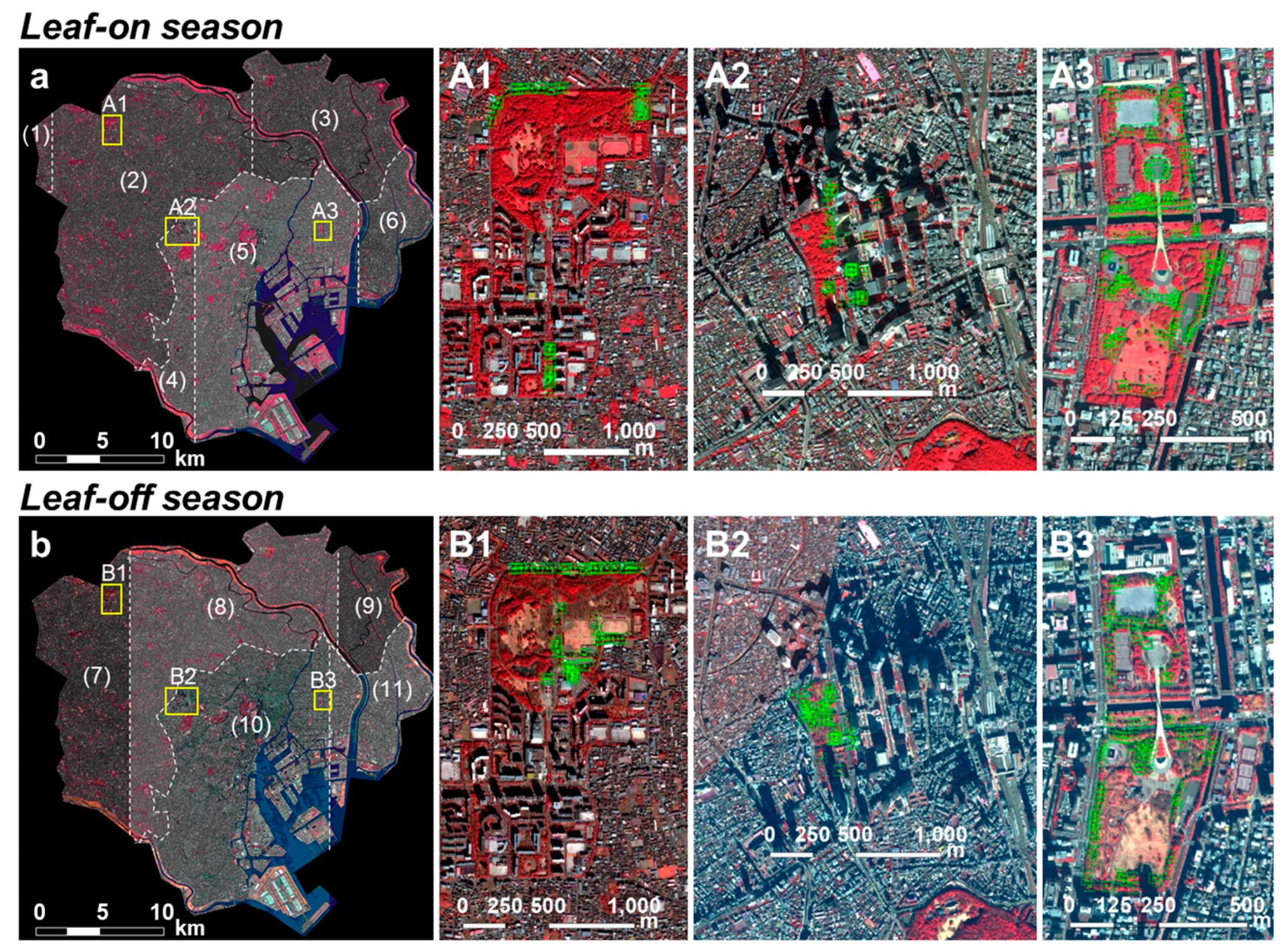
Figure 1. (a) Study area superimposed on the population density map of Tokyo according to the 2015 National Population Census. The area surrounded by the black lines with high population density indicates our study area of 23 municipalities (Tokyo special wards). (b) Location and name of each municipality (special ward). The maps were generated using MATLAB R2018b.
Remotesensing 12 01505 g001
Figure 2. WorldView-2/3 imagery used in this study for (upper panels: (a) leaf-on season and (lower panels: (b) leaf-off season. The yellow areas in (a) and (b), respectively, represent the sites where leaf area index (LAI; m2 m−2) field measurement was conducted in each season (A1A3 and B1B3). The green plots illustrate the LAI field measurement points. Aerial photograph inspection in (A2 and B2) and field investigation in (A3 and B3) were conducted to assess the accuracy of tree mapping results from WorldView-2/3 imagery. Satellite imagery from DigitalGlobe Products. (a, A1, b, and B1B3) WorldView2 © 2020 DigitalGlobe, Inc., a Maxar company. (a, A2, and B3) WorldView3 © 2020 DigitalGlobe, Inc., a Maxar company.
Remotesensing 12 01505 g002
Figure 3. Flowchart of pixel-based image classification procedure for tree canopy cover extraction.
Remotesensing 12 01505 g003
Figure 4. Mapping results of vegetation in the test area shown in Figure 2 (A2 and B2) for leaf-on season (upper panels: a1a3) and leaf-off season (lower panels: b1b3). The areas enclosed by yellow lines are places where the comparisons were performed. (a1) Aerial photograph taken in May 2012 (leaf-on season). (a2) Tree canopy cover (purple) and grass (green) based on the Tokyo Green and Water Coverage ratios data (Tokyo GWC-ratio data) derived from aerial photograph interpretation. (b1) Aerial photograph taken in March 2013 (leaf-off season). (b2) Manually delineated tree canopy cover (red) and grass (green). (a3 and b3) Tree canopy cover (red), grass (dense = green; sparse = light blue), and vegetation in shadow (blue) from the WorldView-2/3 imagery. Satellite imagery from DigitalGlobe Products. (a2 and a3) WorldView3 © 2020 DigitalGlobe, Inc., a Maxar company. (b3) WorldView2 © 2020 DigitalGlobe, Inc., a Maxar company. (a1, b1, and b2) Aerial photograph © NTT GEOSPACE CORPORATION.
Remotesensing 12 01505 g004
Figure 5. Mapping results of vegetation in the test area shown in Figure 2 (A3 and B3). (a1) Map of the tree canopy (purple) and grass (green) based on the Tokyo GWC-ratio data. (b1) Vegetation cover, which was manually delineated based on field observations. (a2 and b2) Vegetation cover estimated from WorldView-2/3 imagery. The areas enclosed by yellow lines represent where the comparisons were performed. Satellite imagery from DigitalGlobe Products. (a1 and a2) WorldView3 © 2020 DigitalGlobe, Inc., a Maxar company. (b1 and b2) WorldView2 © 2020 DigitalGlobe, Inc., a Maxar company.
Remotesensing 12 01505 g005
Figure 6. Image classification performance for tree canopy cover estimation. The plots represent the ratio of tree canopy cover (%) estimated for various areas (two test areas, each of 23 municipalities in Tokyo special-wards, and all Tokyo special wards) in comparison with the respective verification data derived from the field survey and aerial photographs.
Remotesensing 12 01505 g006
Figure 7. Performance of the LAI−NDVI (Normalized Difference Vegetation Index) approximate model developed for both the leaf-on and leaf-off seasons. (a1 and b1) Scatter plots of vegetation index (NDVI) vs. observed leaf area index (LAI; m2 m−2). The line represents the LAI−NDVI approximate model derived from the maximum NDVI and observed LAI data. (a2 and b2) Estimated LAI vs. observed LAI. The y = 1.00x line is fitted. (c) Box plots of comparison between observed LAI and estimated LAI for each species.
Remotesensing 12 01505 g007
Figure 8. Example of mapping results of tree canopy leaf area in the test area shown in Figure 2 (A1 and B1). (a) Vegetation cover according to the Tokyo GWC-ratio data based on aerial photograph. Estimated map of tree leaf area index (LAI; m2 m−2) for leaf-on season (b) and leaf-off season (c). Satellite imagery from DigitalGlobe Products. (ac) WorldView2 © 2020 DigitalGlobe, Inc., a Maxar company.
Remotesensing 12 01505 g008
Table 1. Detailed information on WorldView-2/3 imagery used in this study.
Phenological
Image Category
SatellitePhotographed DateSolar Azimuth Angle (Deg)Solar Altitude (Deg)Observation Angle
(In Track) (Deg)
Observation Angle (Cross Track) (Deg)Image Location in Figure 2
Leaf-on seasonWorldView-218 October 2016162.343.1−2.83.0(1)
WorldView-226 October 2016165.140.7−2.3−5.1(2)
WorldView-226 October 2016165.240.79.1−5.4(3)
WorldView-313 October 2013164.145.511.518.8(4)
WorldView-322 September 2014150.751.2−7.4−3.2(5)
WorldView-201 November 2015167.739.413.7−6.8(6)
Leaf-off seasonWorldView-214 February 2017156.638.46.0−3.2(7)
WorldView-204 April 2017147.156.0−8.210.8(8)
WorldView-221 January 2016158.131.3−8.3−4.1(9)
WorldView-213 January 2014165.431.716.5−4.9(10)
WorldView-221 February 2013162.842.47.1−10.8(11)
Table 2. Vegetation indices considered in this study that concern prediction of leaf area index (LAI).
Vegetation IndicesAlgorithmAbbreviationReference
Normalized Difference Vegetation Index(NIRred)/(NIR + red)NDVI[27]
Red Edge NDVI(NIRRed edge)/(NIR + Red edge)RE−NDVI[28]
Wide Dynamic Range Vegetation Index(0.1 × NIRRed)/(0.1 × NIR + Red)WDRVI1[29]
Wide Dynamic Range Vegetation Index(0.2 × NIRRed)/(0.2 × NIR + Red)WDRVI2[29]
2-Band Enhanced Vegetation Index2.5 × (NIRRed)/(NIR + 2.4 × Red + 1)EVI2[30]
Table 3. Band combinations and threshold variables determined for image classification.
Classification StepClassification CategoryNormal Differential Index (NDI)ThresholdSeasonImage No. In Figure 2
1(high NDVI)/(low NDVI) B a n d 5 B a n d 7 B a n d 5 + B a n d 7 −0.28leaf-on(1)–(6)
leaf-off(7)–(11)
2(vegetation)/(high NDVI non-vegetation) B a n d 5 B a n d 6 B a n d 5 + B a n d 6 −0.12leaf-on(1)–(6)
leaf-off(7)–(11)
3(tree canopy)/(grass) B a n d 1 B a n d 3 B a n d 1 + B a n d 3 0.2leaf-on(1)–(6)
leaf-off(7)–(11)
4(dense grass)/(sparse grass) B a n d 5 B a n d 8 B a n d 5 + B a n d 8 −0.58leaf-on(1)–(6)
leaf-off(7)–(11)
5(non-vegetation in sunlight)/(shadow and water) B a n d 1 B a n d 6 B a n d 1 + B a n d 6 0.45leaf-on(1)–(6)
leaf-off(7)–(11)
6(shaded vegetation)/(shaded non-vegetation) B a n d 5 B a n d 7 B a n d 5 + B a n d 7 0.01
0.02
0.11
0.14
leaf-on(1) and (2)
(3)–(6)
leaf-off(7)–(9)
(10) and (11)
Table 4. Classification accuracy of tree canopy cover (%) from WorldView-2/3 imagery for two test areas in Figure 4 and Figure 5.
RegionAreaSeasonTree Canopy Cover RatioDifference
WorldView-2/3 imagery Field investigationTokyo GWC-ratio data
Figure 40.3 km2Leaf-on42.4%36.9%5.5%
Leaf-off22.0%24.0%2.0%
WorldView-2/3 imageryAerial photographTokyo GWC-ratio data
Figure 53.0 km2Leaf-on11.9%8.4%3.5%
Leaf-off7.5%6.8%0.7%
Table 5. Comparison of the total tree canopy leaf area (km2) estimated in Figure 8 and all Tokyo special wards from the satellite images (WorldView-2/3, Landsat5-TM, and Landsat8) and the respective LAI−VI models.
SatelliteImagery DateEntire Region
of Figure 8
Tree Colony Region in Figure 8All Tokyo Special WardsLAI−VI modelRef
Leaf AreaMean LAI ± SDLeaf AreaMean LAI ± SDLeaf AreaMean LAI ± SD
(km2)(m2 m−2)(km2)(m2 m−2)(km2)(m2 m−2)
WorldView-2*4.42.4 ± 2.40.25.5 ± 1.4632.61.1 ± 1.6 L A I = 0.100 e N D V I / 0.179
(NDVI range: 0–0.8)
4.82.6 ± 3.20.36.8 ± 2.9632.81.0 ± 1.8 L A I = 27.5 e W D R V I 1 / 0.167
(WDRVI1 range: < −0.15)
4.82.6 ± 3.00.26.4 ± 2.4648.71.0 ± 1.7 L A I = 4.0 e W D R V I 2 / 0.217
(WDRVI2 range: < 0.2)
4.62.5 ± 3.00.26.5 ± 2.3553.20.9 ± 1.8 L A I = 0.05 e E V I 2 / 0.307
(EVI2 range: 0–1.6)
Landsat5-TM11 October 20102.31.2 ± 1.20.14.0 ± 0.4298.00.5 ± 0.5 L A I = 0.419 e N D V I / 0.27 [2]
Landsat827 October 20161.30.7 ± 0.80.12.4 ± 0.2104.00.2 ± 0.4 L A I = 3.44 e N D V I 3.38
(LAI range: > 0)
[3]

