Forest Inventory with Long Range and High-Speed Personal Laser Scanning (PLS) and Simultaneous Localization and Mapping (SLAM) Technology

Abstract

The use of new and modern sensors in forest inventory has become increasingly efficient. Nevertheless, the majority of forest inventory data are still collected manually, as part of field surveys. The reason for this is the sometimes time-consuming and incomplete data acquisition with static terrestrial laser scanning (TLS). The use of personal laser scanning (PLS) can reduce these disadvantages. In this study, we assess a new personal laser scanner and compare it with a TLS approach for the estimation of tree position and diameter in a wide range of forest types and structures. Traditionally collected forest inventory data are used as reference. A new density-based algorithm for position finding and diameter estimation is developed. In addition, several methods for diameter fitting are compared. For circular sample plots with a maximum radius of 20 m and lower diameter at breast height (dbh) threshold of 5 cm, tree mapping showed a detection of 96% for PLS and 78.5% for TLS. Using plot radii of 20 m, 15 m, and 10 m, as well as a lower dbh threshold of 10 cm, the respective detection rates for PLS were 98.76%, 98.95%, and 99.48%, while those for TLS were considerably lower (86.32%, 93.81%, and 98.35%, respectively), especially for larger sample plots. The root mean square error (RMSE) of the best dbh measurement was 2.32 cm (12.01%) for PLS and 2.55 cm (13.19%) for TLS. The highest precision of PLS and TLS, in terms of bias, were 0.21 cm (1.09%) and −0.74 cm (−3.83%), respectively. The data acquisition time for PLS took approximately 10.96 min per sample plot, 4.7 times faster than that for TLS. We conclude that the proposed PLS method is capable of efficient data capture and can detect the largest number of trees with a sufficient dbh accuracy.

1. Introduction

The management of natural resources and complex ecosystems such as forests requires reliable information and data, in order to make well-founded and transparent decisions. The major purpose of forest inventories is to provide relevant information on the status and changes of forest landscapes. The need for information from forest inventories has increased steadily in recent decades [1] and, in order to provide reliable and precise information on traditional attributes such as average growing stock timber volume or tree count, measurement errors (besides the design-based sampling variance) should be kept as small as possible. Forest inventory data are not only required for decision making in forest management, but are also used as an empirical platform for manifold research activities.

Tree location and diameter at breast height (dbh) are crucial parameters in forest inventory. Traditional methods based on field inventory work [2,3,4,5] for tree location calculation and dbh measurement are labor intensive, time consuming, prone to manifold measurement errors [6,7,8], and are thus limited in their spatial extent. The lack of efficient inventory tools is an old and well-known challenge related to forest in-situ measurements [9] and, so, since the beginning of forest inventory, trials to improve efficiency have permanently enhanced techniques, instruments, and protocols [7]. Nevertheless, these traditionally collected data are often used as reference values for the quality assessment of automatic sensor-based forest inventories.

In recent years, technologies from different platforms, such as the point clouds from terrestrial laser scanning (TLS) (e.g., [6,8,9,10,11,12,13,14,15,16,17,18,19,20]) and images (e.g., [9,21,22,23,24,25,26,27]), have presented feasible options for applying automated measurements of forest attributes, which have the capacity to provide three-dimensional (3D) forest structure data accurately and automatically. Airborne laser scanning (ALS) (e.g., [28,29,30,31,32]), unmanned aerial vehicle (UAV) laser scanning (ULS) (e.g., [33,34,35,36,37,38]), and UAV images (e.g., [34,38,39,40,41]) feature the ability to cover large areas (up to regional level) and to penetrate gaps between vegetation foliage. However, ALS (and, partly, UAV) systems are generally unsuitable for deriving accurate and detailed information of individual trees, such as tree position at breast height and dbh, as their three-dimensional (3D) point clouds represent tree stems too sparsely and the derived information largely depends on the quality and quantity of field reference data [42,43].

To further improve the efficiency of data collection using laser scanning systems, mobile laser scanning (MLS) has been used in forestry surveys, due to its ability to measure complex forest areas in a short time [9,42,44,45,46,47]. With TLS, it is necessary to have multiple scan positions (i.e., a multi-scan approach) with artificial targets for high detection rates and low dbh errors; even then, there are always shadowing effects and non-detections [6,20,48]. In comparison to TLS, MLS offers a powerful tool to solve the problem of tree occlusion and inability to move. This reduces the required time and labor costs. Liang et al. [42] reported that, within an equal time frame, the area that can be investigated by utilizing MLS is significantly larger than the area investigated with TLS. However, the data acquired by MLS is often less precise than TLS point cloud data, due to the propagation of positioning errors within MLS point cloud data [42,47]. Some studies have also reported that the point clouds acquired with the MLS were much noisier [49].

An MLS system consists of one or several laser scanner(s) and multi-sensor positioning and orientation sensors. The carrier platforms typically used for terrestrial MLS in forestry are vehicles [9,45,50], backpacks [45,51,52,53], or handheld systems [46,47,49,53,54,55,56,57,58]. A typical MLS system uses a Global Navigation Satellite System (GNSS) receiver and an inertial measurement unit (IMU) for positioning and orientation. This configuration limits their use to relatively open environments, such as highways and infrastructure corridors [46,47,49,54,55]. When using GNSS MLS in the forest, weak or missing GNSS signals under the canopy has become the greatest challenge for the application of MLS in forestry surveys [47,59]. The latest MLS systems, especially for hand-held devices, are capable of digitalizing complex 3D scenarios on the move without GNSS. Using simultaneous localization and mapping (SLAM) algorithms, simultaneous point cloud registration and map extraction is done. Regarding the quality of the data, these devices usually offer a centimeter-level accuracy and a resolution that depends on the acquisition speed and the distance to the object at each moment [54]. Chen et al. [47] stated that SLAM-based MLS has the potential to improve mapping efficiency compared with conventional field measurements, as well as to compensate for the limitations of other laser scanning techniques, such as having to transport the scanner and associated equipment from site to site, which is one the major disadvantage of TLS. In addition, for SLAM MLS, there is no need for certain terrain conditions and GNSS signals, which limit the application of MLS [60].

To our best knowledge, there are currently only a few studies on the use of hand-held SLAM MLS systems in forest inventory for measuring tree position and dbh. The major findings of selected recent studies are described as follows. First of all, the different terms for SLAM-based MLS systems have to be brought into accordance. Most studies [46,49,55,56,57] have used the term handheld mobile laser scanner (HMLS). However, there are also terms such as wearable laser scanning (WLS) [54], handheld laser scanner (HLS) [53], and personal laser scanning (PLS) [47]. We use the term personal laser scanning (PLS) in this study.

Only three different SLAM-based PLS-devices have so far been used in forest inventory related studies: the ZEB1 [46], ZEB-REVO [61], and ZEB-REVO-RT [62] (all GeoSLAM Ltd., Nottingham, UK). ZEB1 [46] was introduced in 2013, which has a spring-mounted sensor head and a data acquisition rate of 43,200 points s^-1 at a maximum range of 30 m. Ryding et al. [46] evaluated ZEB1 against multi-scan TLS. Fewer trees were detected with ZEB1 (omission difference between 8% and 11%) and the root mean square error (RMSE) of the ZEB1-based stem positioning ranged between 1.9 cm (17%) and 3.5 cm (29%) when using TLS data as reference. The corresponding bias was between 0 cm (−0.3%) and 0.5 cm (−4.6%). Oveland et al. [53] compared the tree detection rates of single-scan TLS (61.8%), ZEB1 (74%), and a backpack mobile laser scanner (87.5%). The associated bias and RMSE of the dbh estimation were −2 cm, 0.3 cm, 0.1 cm, and 6.2 cm, 3.1 cm, 2.2 cm, respectively. Giannetti et al. [56] reported RMSE of 1.28 cm for ZEB1 and 1.13 cm for TLS-based dbh measurements, where the corresponding bias was -0.38 cm and -0.41 cm, respectively. Bauwens et al. [49] reported detection rates for single-scan TLS (78%), multi-scan TLS (93%), and ZEB1 (90%). The bias of the dbh measurements was −0.17 cm for multi-scan TLS and −0.08 cm for ZEB1, and the corresponding RMSE was 1.3 cm (4.7%) and 1.11 cm (4.1%), respectively.

The successors ZEB-REVO [61] and ZEB-REVO-RT [62] were introduced in 2015 and 2017, respectively, which had the same type of rotating sensor head (270° × 360° angular field of view) and data acquisition rate and maximum range of 43,200 points s⁻¹ and 30 m, respectively. The difference between these two models is real time-data visualization, which is only offered by the ZEB-REVO-RT. Chen et al. [47] used ZEB-REVO-RT and were able to detect 93.3% of tree positions, where the RMSE of dbh measurements was 1.58 cm. Cabo et al. [54] showed that the performance of ZEB-REVO-based dbh measurement (RMSE 0.9–1.1 cm) was equivalent to that of TLS; there was no apparent differences in tree detection nor significant bias in dbh estimation. Vatandaşlar and Zeybek [57] found that ZEB-REVO-collected 3D data yielded slightly higher dbh values than conventional ground measurements. However, its correlation coefficients ranged between 0.978 and 0.998.

Similar to TLS, where the number and geometric setup of scan positions is important for tree detection and diameter estimation [20,63], the selection of a walking path is a crucial task for PLS applications. In connection with the SLAM algorithm, it is often mentioned that each scan should start and end at a same fixed point to ensure a closed loop. Bauwens et al. [49] stated that the path in PLS should be designed to have (1) a good distribution of the scanning positions (i.e., the plot is crossed four times and the path assures that the plot border is scanned at least once); (2) a pattern which reduces scanner range noise; and (3) avoids problems associated with drift, which can occur if the SLAM algorithm does not result in good alignment. Similar to Bauwens et al. [49], Oveland et al. [53] and Giannetti et al. [56] used star-shaped walking paths to minimize occluded areas and used the same start and end point. Ryding et al. [46] chose a free walking method to cover a subplot and, where possible, the user walked in “straight lines” up and down (obstacles were avoided) with the instrument remaining at breast height throughout. To assess the influence of scan density on accuracy estimation, three different survey paths were tested by Del Perugia et al. [55]. They found that walking around each tree improved the detection of the trees with small diameters; however, this is relatively time-consuming. Furthermore, walking back and forth along straight lines drawn at a distance of 10 m from each other has been shown to provide sufficient data to assess single-tree attributes, such as tree position and dbh [55].

The goal of the present study was to investigate the accuracy of tree detection and diameter estimation in forest inventory, using a new SLAM-based PLS system under various stand and terrain conditions. We used a ZEB HORIZON (GeoSLAM Ltd., Nottingham, UK) [64] system, which drastically outperforms the existing sensors (i.e., ZEB1, ZEB-REVO, and ZEB-REVO-RT) in terms of data acquisition rate (300,000 points s⁻¹ vs. 43,200 points s⁻¹) and max. scanning range (100 m vs. 30 m). According to our best current knowledge, this is the first study on the application of this new scanner in a forest inventory context. Furthermore, we present a new algorithm for the automatic detection of tree stems and compare various methods for automatic dbh measurement. The results of the PLS data were compared with TLS results on the same inventory plots, using the same algorithms for automatic tree detection and dbh estimation. Manual measurements on the sample plots were used as reference data. In addition, cylindrical reference objects were scanned to test the diameter accuracy of PLS and TLS under non-forest conditions.

The point clouds and reference data used in this study are freely available (Creative Commons Attribution 4.0 International License - CC BY 4.0) under doi: 10.5281/zenodo.3698956 (https://0-doi-org.brum.beds.ac.uk/10.5281/zenodo.3698956). (see Supplementary Materials)

2. Data and Methods

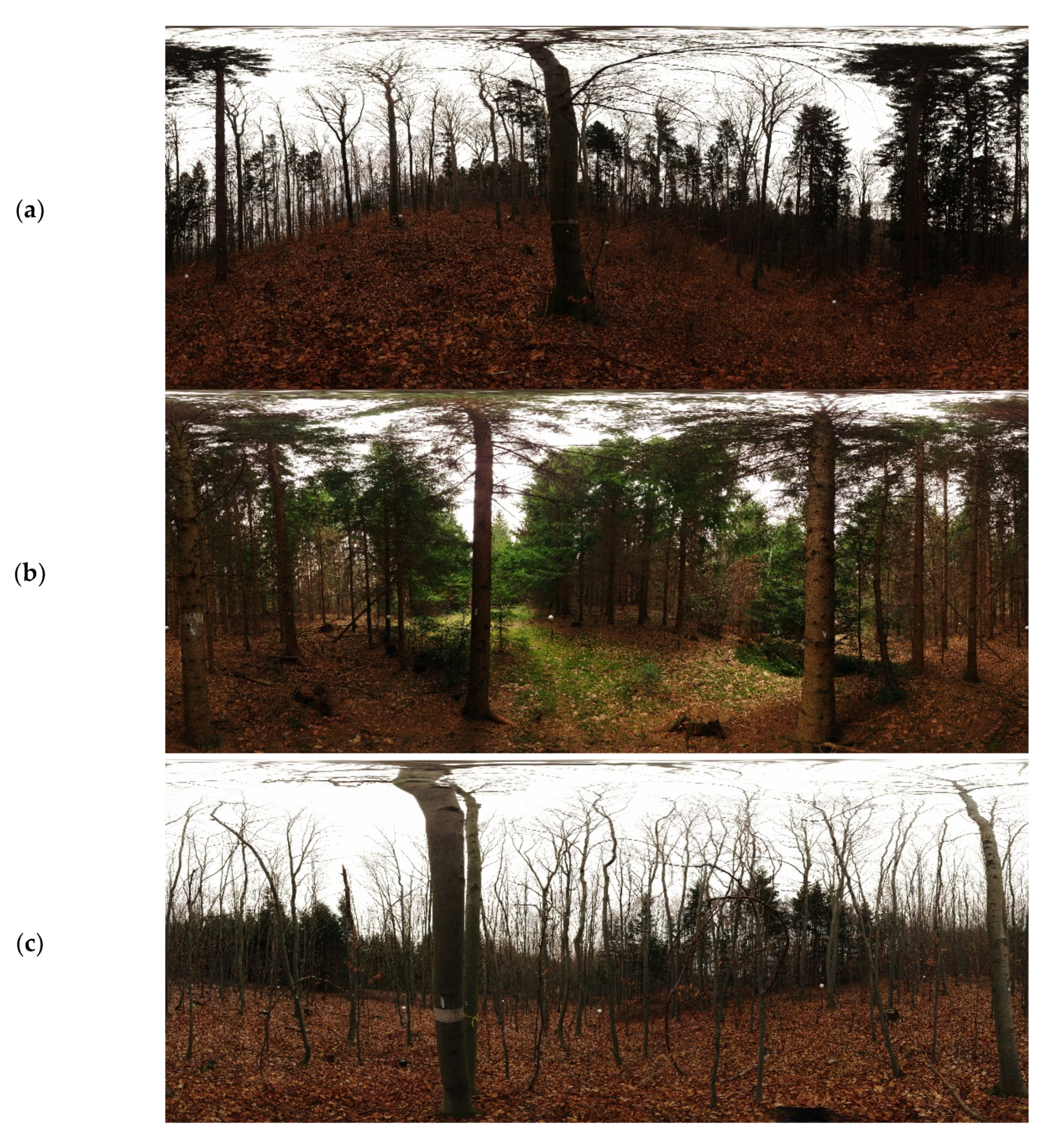
2.1. Study Area and Sample Plots

Since 1989, the Institute of Forest Growth has maintained a permanently repeated forest inventory in the forest district of Ofenbach, located in the federal state of Lower Austria near the village of Forchtenstein [65]. A total of 554 sample plots are systematically aligned in a regular grid with a mesh width of 141.4 m $\times$ 141.4 m. At each sample point, Bitterlich relascope sampling (synonymously, angle count sampling) [66,67,68] was conducted using a constant basal area factor of k = 4 m² ha⁻¹. Trees were recorded only if their diameter at breast height (dbh) is greater than or equal to a lower threshold of 5 cm, and if their distance to the plot center $\mathrm{R}\le 50\times \mathrm{dbh}/2$. Thus, the Bitterlich method produces an incomplete pattern of spatial tree positions resulting from a size-related and distance-dependent thinning.

For the present study, a subsample of 20 plots was selected in such a way that the variation in forest type (broadleaved, coniferous, and mixed), forest structure (one- or two-layered), and terrain property (flat to steep) was represented. In order to obtain reference information for the trees that were not included in the Bitterlich sample, additional manual measurements were conducted in the field in March 2019. The tree positions, dbh (measured from one direction at 1.3 m height) and species of all trees with a dbh of 5 cm or greater and a distance of 20 m or less from the sample plot center were collected [20].

In addition, covariates were derived for each sample plot: among these are stand class, existence of regeneration, proportion of main species, terrain slope, basal area per hectare ($BA/ha$), quadratic mean diameter ($dm$), stand density index ($SDI$) [69], stem density in terms of number of trees per hectare ($N/ha$), coefficient of variation of diameter at breast height ($CVdbh$), dbh differentiation according to Füldner [70] ($Diff\_Fuel$), Clark and Evans aggregation index [71] ($CE$), and Shannon index [72].

Table 1. Summary statistics of sample plots. $slope$, slope of sample plot; $dm$, diameter of mean basal area tree; $BA/ha$, basal area per hectare; $N/ha$, number of trees per hectare; $SDI$, stand density index; $CVdbh$, coefficient of variation of diameter at breast height; $Diff\_Fuel$, dbh differentiation according to Füldner; $CE$, Clark and Evans aggregation index; $shannon$, Shannon index.

# of sample plots	20
# of trees	2466
# of trees/sample plot	123.3
dbh range (cm)	5.0–74.0
	Mean	SD	Min	Max	q(0.05)	q(0.25)	q(0.5)	q(0.75)	q(0.95)
$slope$ (%)	29.4	10.2	10.5	51.0	14.0	22.4	29.1	34.3	47.3
$dm$ (cm)	27.0	9.1	12.1	43.1	13.4	20.2	27.2	32.8	41.9
$BA/ha$ (m2/ha)	39.6	8.0	26.8	56.9	26.8	32.9	39.8	43.9	51.7
$N/ha$ (trees/ha)	981	807	239	3350	284	483	689	1218	2383
$SDI$ (trees/ha)	802	174	535	1246	545	717	772	935	1009
$CVdbh$	0.53	0.13	0.25	0.74	0.34	0.45	0.54	0.63	0.71
$Diff\_Fuel$	0.41	0.08	0.20	0.52	0.29	0.35	0.40	0.47	0.50
$CE$	0.93	0.12	0.71	1.14	0.79	0.85	0.93	0.99	1.13
$shannon$	0.79	0.28	0.15	1.20	0.38	0.61	0.81	0.98	1.15

shows summary statistics (number of trees, mean, standard deviation, min, and max) of the metric sample plot parameters. A complete description of the 20 sample plots can be found in Appendix A,

Table A1. Plot descriptions of the 20 sample plots and summary statistics of sample plots. $slope$, slope of sample plot; $p\_spr$, proportion of Norway spruce; $p\_bee$, proportion of Common beech; $p\_lar$, proportion of European larch; $p\_pin$, proportion of Scots pine; $p\_fir$, proportion of Silver fir; $dm$, diameter of mean basal area tree; $BA/ha$, basal area per hectare; $N/ha$, number of trees per hectare; $SDI$, stand density index; $CVdbh$, coefficient of variation of diameter at breast height; $Diff\_Fuel$, dbh differentiation according to Füldner; $CE$, Clark and Evans aggregation index; $shannon$, Shannon index; PLS/TLS, used scanner device.

Plot	Stand Class	Regen- eration	$\mathit{s}\mathit{l}\mathit{o}\mathit{p}\mathit{e} (\%)$	$\mathit{p}\_\mathit{s}\mathit{p}\mathit{r} (\%)$	$\mathit{p}\_\mathit{b}\mathit{e}\mathit{e} (\%)$	$\mathit{p}\_\mathit{l}\mathit{a}\mathit{r} (\%)$	$\mathit{p}\_\mathit{p}\mathit{i}\mathit{n} (\%)$	$\mathit{p}\_\mathit{f}\mathit{i}\mathit{r} (\%)$	$\mathit{d}\mathit{m} \left(\mathbf{cm}\right)$	dbh Range (cm)	$\mathit{B}\mathit{A}/\mathit{h}\mathit{a} ({\mathbf{m}}^2/\mathbf{ha})$	$\mathit{N}/\mathit{h}\mathit{a} (\mathbf{trees}/\mathbf{ha})$	$\mathit{S}\mathit{D}\mathit{I} (\mathbf{trees}/\mathbf{ha})$	$\mathit{C}\mathit{V}\mathit{d}\mathit{b}\mathit{h}$	$\mathit{D}\mathit{i}\mathit{f}\mathit{f}\_\mathit{F}\mathit{u}\mathit{e}\mathit{l}$	$\mathit{C}\mathit{E}$	$\mathit{S}\mathit{h}\mathit{a}\mathit{n}\mathit{n}\mathit{o}\mathit{n}$	PLS/TLS
1	2	1	27.4	5	86	3	3	1	25.7	5.3–54.4	38.4	740	774	0.71	0.52	0.85	0.61	PLS/TLS
2	3	2	22.4	9	73	4	2	5	32.3	7.0–49.5	37.2	454	685	0.34	0.38	0.93	0.98	PLS
3	3	4	32.5	37	47	0	3	7	41.8	16.0–58.0	32.8	239	546	0.25	0.20	1.14	1.20	PLS/TLS
4	2	1	24.0	58	11	31	0	0	28.1	5.2–57.3	39.5	637	768	0.65	0.31	1.13	0.92	PLS/TLS
5	1	0	22.4	26	71	3	0	0	15.0	5.0–42.5	40.0	2260	997	0.5	0.36	0.83	0.73	PLS/TLS
6	1	0	34.2	14	86	0	0	0	12.1	5.0–32.4	26.8	2332	727	0.46	0.33	0.93	0.43	PLS/TLS
7	3	3	22.4	35	50	3	6	6	38.3	6.8–62.0	32.9	286	567	0.52	0.40	0.99	1.15	PLS/TLS
8	1	1	10.5	82	10	1	0	5	18.7	5.0–50.7	32.9	1202	752	0.48	0.37	0.99	0.69	PLS/TLS
9	1	0	51.0	60	39	0	0	0	13.5	5.0–28.2	47.9	3350	1246	0.42	0.33	1.03	0.69	PLS/TLS
10	2	0	47.1	13	87	0	0	0	26.3	5.0–49.6	26.8	493	535	0.57	0.50	0.96	0.39	PLS/TLS
11	3	3	24.0	71	29	0	0	0	43.1	5.4–74.0	56.9	390	934	0.40	0.30	1.12	0.60	PLS/TLS
12	3	1	14.2	56	38	0	0	5	35.2	5.8–59.1	43.3	446	770	0.47	0.40	0.89	0.85	PLS/TLS
13	2	0	34.2	41	57	0	0	0	21.1	5.1–42.0	44.4	1265	966	0.68	0.48	0.84	0.78	PLS/TLS
14	2	0	41.4	35	56	1	6	1	32.0	6.6–55.4	43.7	541	806	0.43	0.39	0.98	0.98	PLS/TLS
15	2	0	25.7	43	45	0	0	0	20.2	5.1–43.7	42.3	1313	936	0.74	0.43	0.80	1.00	PLS/TLS
16	3	1	37.8	26	56	0	0	19	32.7	5.1–56.7	46.7	557	855	0.58	0.47	0.90	0.99	PLS/TLS
17	3	2	20.7	5	53	0	24	18	33.1	5.0–60.2	42.6	493	776	0.56	0.50	0.71	1.13	PLS/TLS
18	2	1	30.8	3	64	0	6	27	28.5	5.4–56.0	51.4	804	993	0.64	0.50	0.93	0.91	PLS/TLS
19	2	0	32.5	0	97	0	3	0	22.6	5.2–43.2	31.1	772	659	0.63	0.47	0.90	0.15	PLS
20	2	0	34.4	4	86	0	0	0	20.2	5.4–44.2	33.8	1050	748	0.59	0.46	0.79	0.57	PLS

Stand class: 1, dbh <22 cm; 2, >50% dbh 22–37 cm; 3, >50% dbh 37–52 cm. Regeneration: 0, no regeneration; 1, <1.3 m; 2, >1.3 m coverage <33%; 3, >1.3 m coverage 33–66%; 4, >1.3 m coverage >66%.

. Panoramic photos of three typical sample plots can be found in Appendix A, Figure A1.

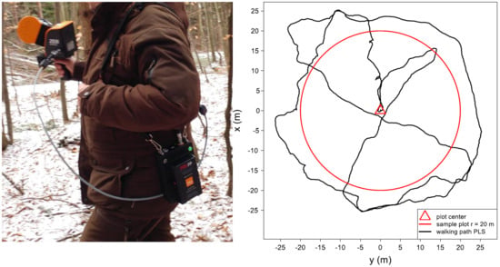
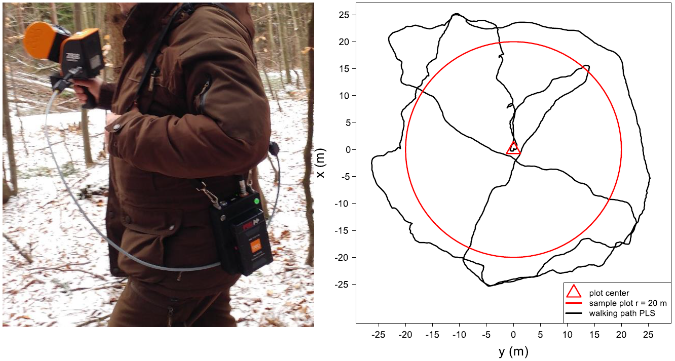
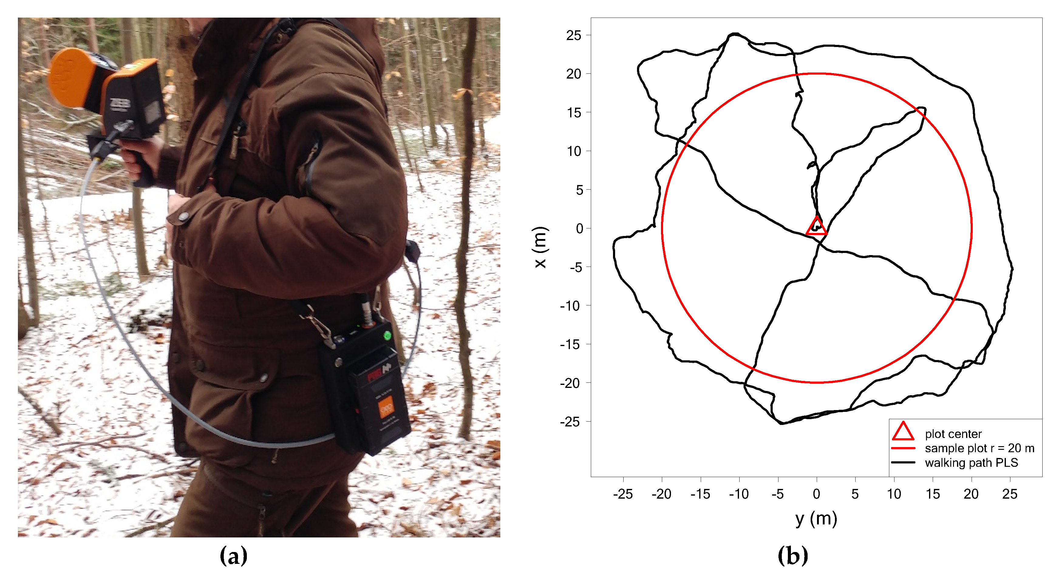
2.2. Instrumentation and Data Collection

A total of 20 sample plots were scanned in March 2019 using a GeoSLAM ZEB HORIZON (GeoSLAM Ltd., Nottingham, UK) [64] personal mobile laser scanner (see Figure 1a). The hand-held part of the device (1.3 kg) includes a VLP-16 (Velodyne LiDAR Inc., Morgan Hill, CA, USA) [73], an optional Firefly 8si camera with 4k resolution, an inertial measurement unit (IMU), and a handle.

The VLP-16 (0.83 kg) has 16 channels and uses time-of-flight Light Detection and Ranging (LIDaR) technology to measure up to 300,000 points per second in single return mode within a maximum range of 100 m. The distances are measured with a continuous wavelength of 903 nm and a range accuracy of ±3 cm. The field of view of the VLP-16 is 360° $\times$ 30° with a vertical angular resolution of 2° and a horizontal angular resolution of 0.1°–0.4°, and the internal rotation rate is 5–20 Hz. The VLP-16 is attached to the ZEB HORIZON by a revolving housing that rotates around an axis orthogonal to the internal rotation axis of the VLP-16 at a rate of 31 min⁻¹. The combination of the internal and external rotation results in an angular field of view of 360° $\times$ 270° [64].

The data logger (2.4 kg) contains the processing unit, a solid-state disk storage (120 GB), and the battery (operational time approx. 3.5 h); this is connected to the hand-held part via a cable. The size of the collected point data is approximately 100–200 MB per minute. A USB 3.0 port on the data logger is used to transfer the data to an external flash drive [64].

Given its battery capacity of approximately 3.5 hours, total weight of 3.7 kg (1.3 kg + 2.4 kg), and compact design (100 mm $\times$ 200 mm $\times$ 240 mm for the hand-held part), the scanner is easy to handle in forestry measurement campaigns. The use of SLAM technology solves the problem of missing or poor GNSS signals under the forest canopy.

Data acquisition with ZEB HORIZON starts with IMU initialization, in order to establish the local coordinate reference system. In the course of this, the scanner was placed on a tripod at the center of the plot. After approximately 15 s of initialization, the survey was executed by moving at walking speed, while the rotating scanner head captured data of the full 3D environment. The 3D data was stored in real time on the hard drive, located in the data logger in GEOSLAM’s proprietary compressed data format. The walking path had a star-shaped design, based on Bauwens et al. [49], for optimal coverage of the plot area, low scanner range noise, and to reduce the drift associated with the SLAM algorithm. Starting from the plot center to the north, the circular sample plot with 20 m radius was circled once with a 2–3 m buffer zone and then crossed twice. The scanner was then placed back (closing the loop) on the tripod at the plot center and the scanning process ended. The recording of the entire sample plots took approximately 7–15 min, depending on the possible walking speed, which differed due to stand and terrain characteristics. There was no need for artificial reference targets. An example of the walking path in a sample plot is presented in Figure 1b.

Out of the 20 PLS scanned sample plots, 17 were scanned in February–March 2018, during the study of Gollob et al. [20], using a FARO Focus3D X330 terrestrial laser scanner (Faro Technologies Inc., Lake Mary, FL, USA). For further information on the scanner and the hardware parameter settings, the reader is referred to Gollob et al. [20].

According to the results of Gollob et al. [20], the multi-scan mode with a scan position in the center and three scan positions at a distance of 15 m in a triangular shape (scan variant 3) was selected as the TLS scan for comparison in this study. The TLS scans were performed with nine Styrofoam spheres as artificial targets and took about 49.6 min (32.6 min scan time without photographs, approx. 12 min scanner installation, and approx. 5 min sphere installation).

2.3. Point Cloud Processing

A step-by-step overview of the entire workflow and detailed parameter settings is given in Appendix A,

Table A2. Workflow and applied software functions and parameters. Black indicates steps for both PLS and TLS. Red indicates steps for PLS solely and blue indicates steps for TLS solely.

Step No.	Step/Substep		Software	Package/Function		Parameters
1	Registration of point cloud		GeoSLAM Hub
2	Export in .las format					100% of points time stamp: scan point color: none
3	Co-registration of scans		FARO SCENE
4	Export in .xyz format
5	Import, transform, and export in .las format		R	data.table, rlas	fread(), write.las()
6	Import data			lidR	readLAS()	filter = "-keep_circle 0 0 21"
7	Classify into ground points and non-ground points				lasground()	csf(class_threshold = 0.05, cloth_resolution = 0.2, rigidness = 1)
8	Create DTM				grid_terrain()	res = 0.2, knnidw(k = 2000, p = 0.5)
9	Normalize relative to DTM				lasnormalize()
10	Remove ground points				lasfilter()	Classification = 1
11	Sample random point per voxel			TreeLS	tlsSample()	voxelize(spacing = 0.02) voxelize(spacing = 0.015)
12a	Clustering 2D	calculate reachability of each point		dbscan	optics()	eps = 0.025 minPts = 90
12b		DBSCAN clustering			extractDBSCAN()	eps_cl = 0.025
13	Filter clusters			various functions in base		nr. of points ≥ 500 nr. of points ≥ 600 vertical extent ≥ 1.3 m
14a	if(extension≥0.22 m²) Clustering 3D	calculate reachability of each point		dbscan	optics()	eps = 0.025 minPts = 20
14b		DBSCAN clustering			extractDBSCAN()	eps_cl = 0.02
14a	if(extension<0.22 m²) Clustering 3D	calculate reachability of each point		dbscan	optics()	eps = 0.025 minPts = 18
14b		DBSCAN clustering			extractDBSCAN()	eps_cl = 0.023
15	Filter clusters			various functions in base		nr. of points ≥ 500 vertical extent ≥ 1.3 m 80% quantile intensity > 7900
16	Stratification into 14 vertical layers			various functions in base		from 1 m to 2.625 m vertical extent = 0.15 m overlap = 0.025 m
17a	Preparing layers for diameter estimation	$d_{circ}$		edci	circMclust()	nx = 25 ny = 25 nr = 5
17b		$d_{ell}$l		conicfit	EllipseDirectFit()
17c		if(diam. <0.3 m) add buffer		various functions in base		+ 0.06 m
17d		if(diam. ≥0.3 m) add buffer		various functions in base		+ 0.09 m
18a	diameter estimation	$d_{circ}$		edci	circMclust()	nx = 25 ny = 25 nr = 5
18b		$d_{ell}$		conicfit	EllipseDirectFit()
18c		$d_{circ2}$		conicfit	LMcircleFit()
18d		$d_{gam}$		mgcv	gam() predict()	s(angle, bs="cc")
				spatstat	area.owin()
18e		$d_{tegam}$		mgcv	gam() predict()	te(angle, Z, bs=c("cc","tp")) Z = 1.3 m
18f				spatstat	area.owin()
19a	Check criteria for diameters for 6 out of 14 layers	sd XY position ($d_{circ}$ and $d_{ell}$)		various functions in base		≤ 0.01 m
19b		sd diameter ($d_{circ}$ and $d_{el}l$)				≤ 0.0185 m
20	Calculate final position at 1.3 m (from $d_{circ}$ or $d_{ell}$)			base	lm()
21	Calculate final dbh at 1.3 m for all diameter fits			base	lm()
22	Affine transformation of tree positions			vec2dtransf	AffineTransform-ation()
23	Assign tree positions			spatstat	pppdist()	cutoff = 0.3
24	Correct bias for dgam			base	lm()

.

When the PLS field data collection was completed, the data was transferred from the data logger to a desktop computer with GeoSLAM Hub 5.2.0 software [74] using a USB flash drive. The GeoSLAM Hub software processed the data automatically with the SLAM algorithm. A moving time window through the raw data was used for scanner location and to calculate the trajectory of the scanner, based on IMU data and feature detection algorithms [46]. Registering of the point cloud was based on the distances and angles of the points relative to the scanner position, using a linearized model to minimize the error in the IMU measurements as well as maximizing the correspondences between the 3D point cloud data for each respective time segment [46]. According to [64], the relative accuracy of points obtained by the ZEB HORIZON is 1–3 cm in the registered point cloud under normal lighting conditions. The registered point cloud is given in a local coordinate system, with origin at the start/end position of the walking path. The data for each of the seventeen sample plots was exported in the LAS file format [75], which is compatible with a variety of point cloud software. For exporting, the parameter settings “100% of points”, “time stamp: scan”, and “point color: none” were selected in GeoSLAM Hub 5.2.0.

Co-registration of the raw TLS scan data was performed manually for each sample plot, by means of Styrofoam reference targets, using the FARO SCENE 6.2 software [76]. A constant cutoff distance of 30 m was chosen for each of the four scanner positions. The aligned scans were then further processed to obtain a complete 3D point cloud for each sample plot. The registered point cloud was in a local coordinate system with origin at the first scan position in the center of the plot. Point clouds were exported separately for each of the seventeen sample plots, in xyz format, as plain text files.

Transforming the local coordinates obtained by PLS and TLS into global coordinates thus only requires a precise measurement of the plot center and a correction of magnetic declination.

In addition to point position measurements, a laser scanner simultaneously measure the energy of the backscattered laser signal and recorde it as an intensity value for each point [77,78,79,80], by internally converting the optical power to voltage by amplifying it in the system, and then transforming it into a scaled integer value named intensity [81]. The intensity values of the two scanners cannot be compared directly, because of a different scaling and because of different laser wavelengths (1550 nm for the FARO Focus3D X330 [82], and 903 nm for the GeoSLAM ZEB HORIZON [64,73]) resulting in a different reflectivity of the surfaces hit by the laser, and thus in a different energy of the backscattered laser signal.

Further point cloud processing and analysis was performed using the statistical computing language R [83]. The TLS point clouds were imported, transformed, and exported in the .las format using the functions fread() and write.las() of the R packages data.table [84] and rlas [85], respectively. Henceforth, the point clouds of PLS and TLS were processed and analyzed with the same algorithms (any differences in the individual parameters can be seen in Appendix A, Table A2). The points were imported and simultaneously clipped to an upright-oriented cylinder with a radius of 21 m centered at the sample plot center using the readLAS() function from the lidR package [86]. Each point cloud was then processed with the lidR lasground() function. By doing so, all points were classified into ground and non-ground points, using a cloth simulation filter algorithm by Zhang et al. [87]. A Digital Terrain Model (DTM) with 20 cm raster resolution was created by interpolating the classified ground points using the grid_terrain() function from lidR. Subsequently, all points were normalized relative to the ground-derived DTM (lasnormalize() from lidR), and the ground points were discarded from the data (lasfilter() from lidR).

2.4. Clustering, Detection of Tree Positions, and dbh Measurement

For automatic tree detection, we further refined the algorithms of Ritter et al. [8] and Gollob et al. [20] based on density-based clustering.

The OPTICS (ordering points to identify the clustering structure) algorithm, developed by Ankerst et al. (1999) [88], was used for clustering. OPTICS is an extension of DBSCAN (density-based spatial clustering of applications with noise) [89], which allows cluster detection in data of varying density (a typical characteristic of TLS and PLS data). DBSCAN requires two parameters: a maximum distance $ϵ$ and a minimum number of points $minPts$. A point $p$ is considered to be a core point of a cluster if its $ϵ$-neighbourhood contains at least $minPts$ points. DBSCAN returns a list of clusters, consisting of core points and points whose $ϵ$-neighbourhood contains core points, but less than $minPts$ points. All other points, which are not reachable from any other point, are considered noise. In the case where $p$ is a core point, a cluster is formed with p together with all points (core or non-core) that are reachable from it. Instead of using a fixed value of $ϵ$, the discrimination of clusters with OPTICS is based on the core distance of every point $p$; that is, the maximum distance value between $p$ and one of its $minPts$ nearest neighbors.

Based on the core distances, for each point $p$, the reachability distance to every other point is calculated. Valleys in these reachability distances represent clusters (the deeper the valley, the more dense the cluster) and high distances indicate points between clusters. The parameter ε is basically unnecessary in OPTICS; however, it improves the computational performance by providing an upper limit for the core distance calculation. Both algorithms (DBSCAN and OPTICS) enable clustering in 2D and 3D space. For full computational details on DBCAN and OPTICS, we refer to Ankerst et al. [88] and Ester et al. [89], respectively. DBSCAN and especially OPTICS have several advantages which justify their selection for clustering point clouds: (i) they are suitable for large databases, (ii) they discover areas of high density and group them into clusters, (iii) they discover clusters of arbitrary shape, (iv) they do not impose any restrictions on the shape of the resulting clusters, (v) they do not require a predetermined number of clusters, and (vi) they can identify noise points [90,91,92].

In order to obtain a lower number of points and a slightly more homogeneous point density for clustering, a random point per voxel at a spatial resolution of 2 cm for PLS data and 1.5 cm for TLS data was sampled from the normalized point cloud using the tlsSample() function from the TreeLS package [93], in order to obtain a comparable point density for PLS and TLS. Subsequently, a vertical layer with an extent of 2 m was clipped and, by discarding the Z values, the points were projected onto a plane. The lower boundary of the layer was placed at 1 m height above ground and the upper boundary of the layer was set at 3 m height. For the remaining points, the reachability of each individual point was calculated using the optics() function from the dbscan package [93]. The parameter eps ($ϵ$) was set to 2.5 cm and parameter minPts ($minPts)$ to 90. Finally, the function extractDBSCAN(), implemented in the dbscan package [93], extracted the DBSCAN clustering [89] by cutting the reachability of the points at eps_cl = 2.5 cm. The points classified as noise were removed, whereby the branch, needle, and regeneration points were largely filtered out. Subsequently, the missing Z values were then merged to the clustered points. Clusters with less than 500 points for PLS (less than 600 points for TLS) or a vertical extent of less than 1.3 m were excluded from further analysis. The further steps were done individually for each cluster. As, in some cases, two or more trees standing close together were classified into a common cluster, an additional cluster step, depending on the horizontal extent (calculated as range of X values $\times$ the range of Y values), was added. If this horizontal extension was greater than or equal to 0.22 m², the parameters eps = 2.5 cm, minPts = 20, and eps_cl = 2 cm were used for optics() and extractDBSCAN(); otherwise (i.e., extension less than 0.22 m²), the parameters eps = 2.5 cm, minPts = 18, and eps_cl = 2.3 cm were used. In contrast to the first cluster step, this clustering was done in 3D. Subsequently, points classified as noise were removed and only clusters with greater or equal than 500 points and a vertical extent of more or equal than 1.3 m remained. Furthermore, the 80% quantile of the intensities was calculated for the PLS data, and only those clusters that had an 80% quantile of intensities greater than 7900 were further analyzed. Through this second cluster step and the intensity filtering (PLS), close-standing trees were segmented and further noise (e.g., branch, needle, and regeneration points) were filtered out.

The 3D point clouds of these clusters were then stratified into 14 vertical layers, each of which had a vertical extent of 15 cm. The lower boundary of the lowest layer was placed at 1 m height above ground, and the lower boundary of the topmost layer was at 2.625 m height. The distance between two neighboring layers was 12.5 cm, resulting in a 2.5 cm overlap of neighboring layers. The 3D points from each layer were projected onto a horizontal plane, creating 2-dimensional XY points. If a layer had less than 50 points, it was excluded from further analysis. Subsequently, circles were separately fitted to the points of each layer using the circular cluster method of Müller and Garlipp [94]. This method has been implemented in the function circMclust() in the R package edci [95]. A regular grid of 25 $\times$ 25 starting points was chosen for the initial circle centers in the optimization. In addition, a sequence of five starting radii, beginning at 1 cm and ending at 50 cm, and with a step width of 9.8 cm, was chosen at each grid point. This procedure resulted in 3125 starting values for each of the 14 layers. Additionally, an ellipse was fitted to the same points as before, using the method of Fitzgibbon et al. [96], which is extremely robust and efficient, as it incorporates an ellipticity constraint into the normalization factor and as it can be solved naturally by a generalized eigensystem. The method has been implemented in the function EllipseDirectFit() in the R package conicfit [97]. These preliminary diameter fits to the thinned point cloud were used to initialize diameter fitting to the original (high-resolution) point cloud. Therefore, the fitted center and shape of the circle (if the circle fit converged) or the ellipse (if the circle fit did not converge) were used to construct a clipping region in the original normalized point cloud (result of Section 2.3., Point Cloud Processing) for each of the 14 layers. To clip out the points, a diameter depending on buffer distance (6 cm for a preliminary diameter estimate of less than 30 cm; 9 cm for a preliminary diameter estimate of 30 cm or more) was added to the radii of the preliminary fitted circles or ellipses.

The final diameters were then calculated based on these clipped points, using the circMclust() and EllipseDirectFit() functions for circular and elliptical fitting, respectively. The ellipse diameter was calculated as the quadratic mean of the ellipse’s two radii. Henceforward, these diameters are referred to as $d_{circ}$ and $d_{ell}$; $d_{ell}$ was only calculated if the ratio of the semi-minor axis to the semi-major axis was greater than or equal to 0.6. Another circle with diameter $d_{circ2}$ was then fitted, using the least-squares-based algorithm of Chernov [98] implemented in the R package conicfit [97]. For this, the center and radii values of $d_{circ}$ or $d_{ell}$ were used as the initial starting radius and initial center, respectively. The stem cross-sections were also modeled using a Generalized Additive Model (GAM) with a smoothing spline (see Figure 2). Thereby, using the above-mentioned center (i.e., from $d_{circ}$ or $d_{ell}$), the Cartesian coordinates were transformed into polar coordinates, including the distance and the angle to the center. The distance to the center was modeled as a function of the angle using a cyclic penalized cubic regression spline smooth (see Figure 2b). This method has been implemented in the function gam() in the R package mgcv [99,100,101,102,103]. The resulting curve was a natural cubic spline through the values at the knots (given two extra conditions specifying that the second derivative of the curve should be zero at the two end knots). The number of knots and the dimension of the basis used to represent the smooth term were chosen by default. The standard deviation of the residuals ($s{d}_{res\_gam}$) was used as a measure of the noise from the point clouds. Distance values were then predicted for 360 angles (from $-\pi$ to $\pi$) and the new polar coordinates were transformed back into Cartesian coordinates (see Figure 2c). Based on this, a polygonal observation window was created and its area was calculated using the functions owin() and area.owin() of the spatstat package [104], respectively. Hereafter, the diameter of a circle with the same area was calculated and referred to as $d_{gam}$. Another diameter was estimated via a tensor product smooth. Therefore, the Cartesian coordinates of the 14 vertical layers (or correspondingly fewer, if less than 50 points were contained in a layer) were transformed into polar coordinates with the use of each layer’s center (from $d_{circ}$ or $d_{ell}$). In contrast to the layered procedure for the previous diameter estimates, it was ensured that there were no vertical overlaps of neighboring layers and the Z coordinates were used (in addition to the angle) to predict the distance. Methodically, this was done with a tensor product smooth implemented in the mgcv package [99,100,101,102,103], using the smooth terms "cc" (cyclic cubic regression spline) and "tp" (thin plate regression spline) for the angle and the Z coordinate, respectively. Distance values were then predicted for 360 angles (from $-\pi$ to $\pi$) and a Z coordinate of 1.3 m. The rest of the process was the same as for $d_{gam}$, and the obtained diameter is referred to as $d_{tegam}$.

After accomplishing the diameter fitting in each vertical layer or for all layers ($d_{tegam}$), the decision as to the tree position was finally proposed as the diameter’s center, determined by the results of the $d_{circ}$ and $d_{ell}$ fits. Trials revealed that this decision could be safely made, depending on the following two criteria. For six out of the 14 total layers: (i) the standard deviation of the XY position coordinates must be less than or equal to 0.01 m, and (ii) the standard deviation of the diameter measurements must be less than or equal to 1.85 cm. The preliminary proposal of a tree location was rejected if at least 1 of the 2 criteria was not met for any of the 3003 total possible combinations of 6 samples from the 14 layers. If several combinations met both criteria, the one with the lowest standard deviation in diameter measurement across the six layers was further analyzed to derive the final tree position and dbh measurement. There were three possibilities for the output: (i) both $d_{circ}$ and $d_{ell}$ had six layers that met the criteria, (ii) only $d_{circ}$ had six layers that met the criteria, and (iii) only $d_{ell}$ had six layers that met the criteria. Based on this, the final tree position was calculated at 1.3 m height using a linear model of the 6 X and Y coordinates over the height. If there were both outputs ($d_{circ}$ and $d_{ell}$) or only $d_{circ}$, then the final tree position was calculated based on the $d_{circ}$ centers. If there was only one output for $d_{ell}$, then the final position was calculated based on this. This means that a final tree position only existed if at least one combination of $d_{circ}$ or $d_{ell}$ met the criteria. A subset of the found tree positions was taken from a circle of 20 m radius around the sample plot center, to be comparable with the reference data. In the same way as for the position, the actual dbh (i.e., $d_{circ}$ and $d_{ell}$) at 1.3 m height was calculated using a linear model. The remaining dbhs (d_circ2, $d_{gam}$, and $d_{tegam}$) were then calculated from the best combinations of $d_{circ}$ and $d_{ell}$ using the heights of the six layers. This means that a final tree dbh for $d_{circ2}$, $d_{gam}$, and $d_{tegam}$ only existed if there was also a final $d_{circ}$ or $d_{ell}$.

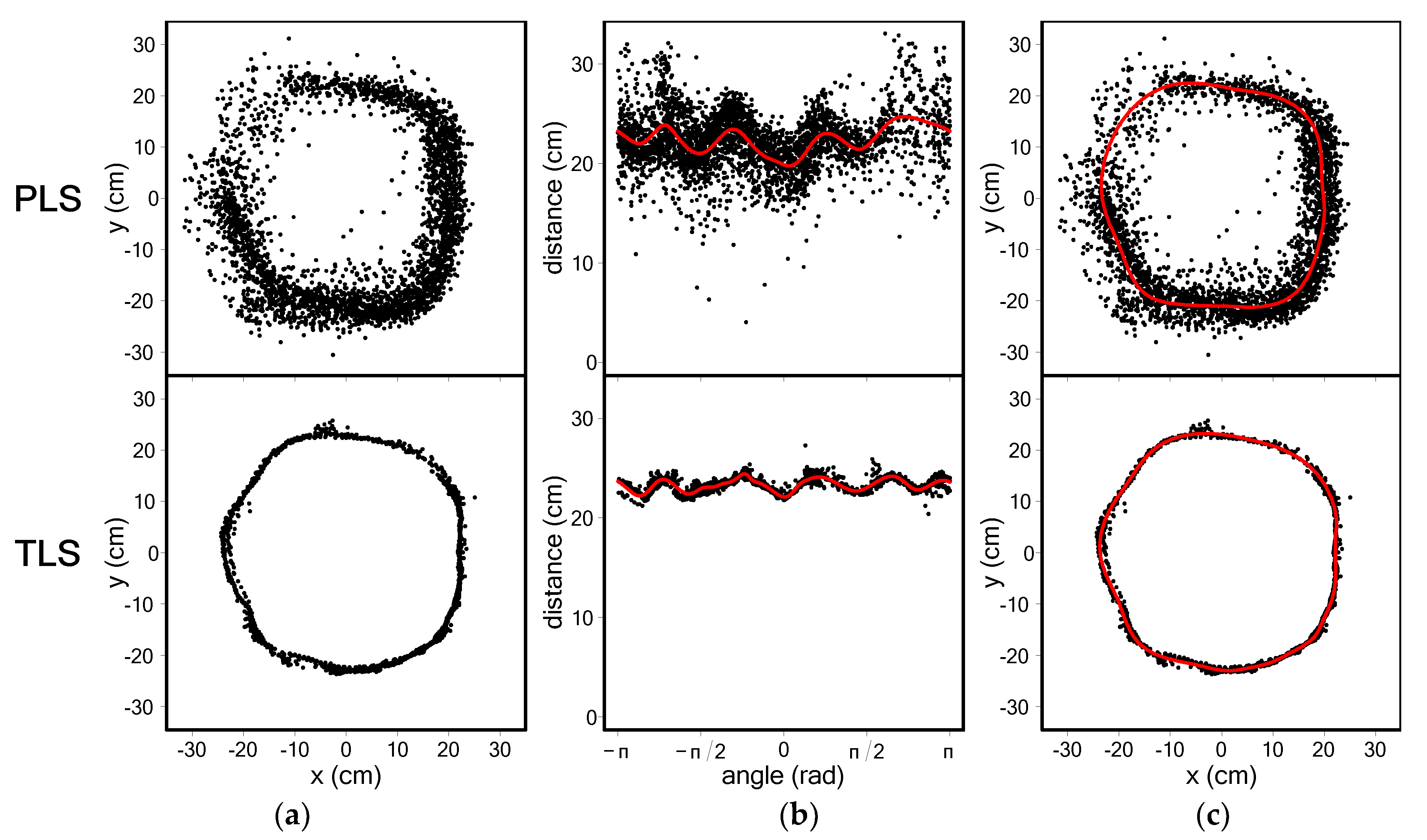
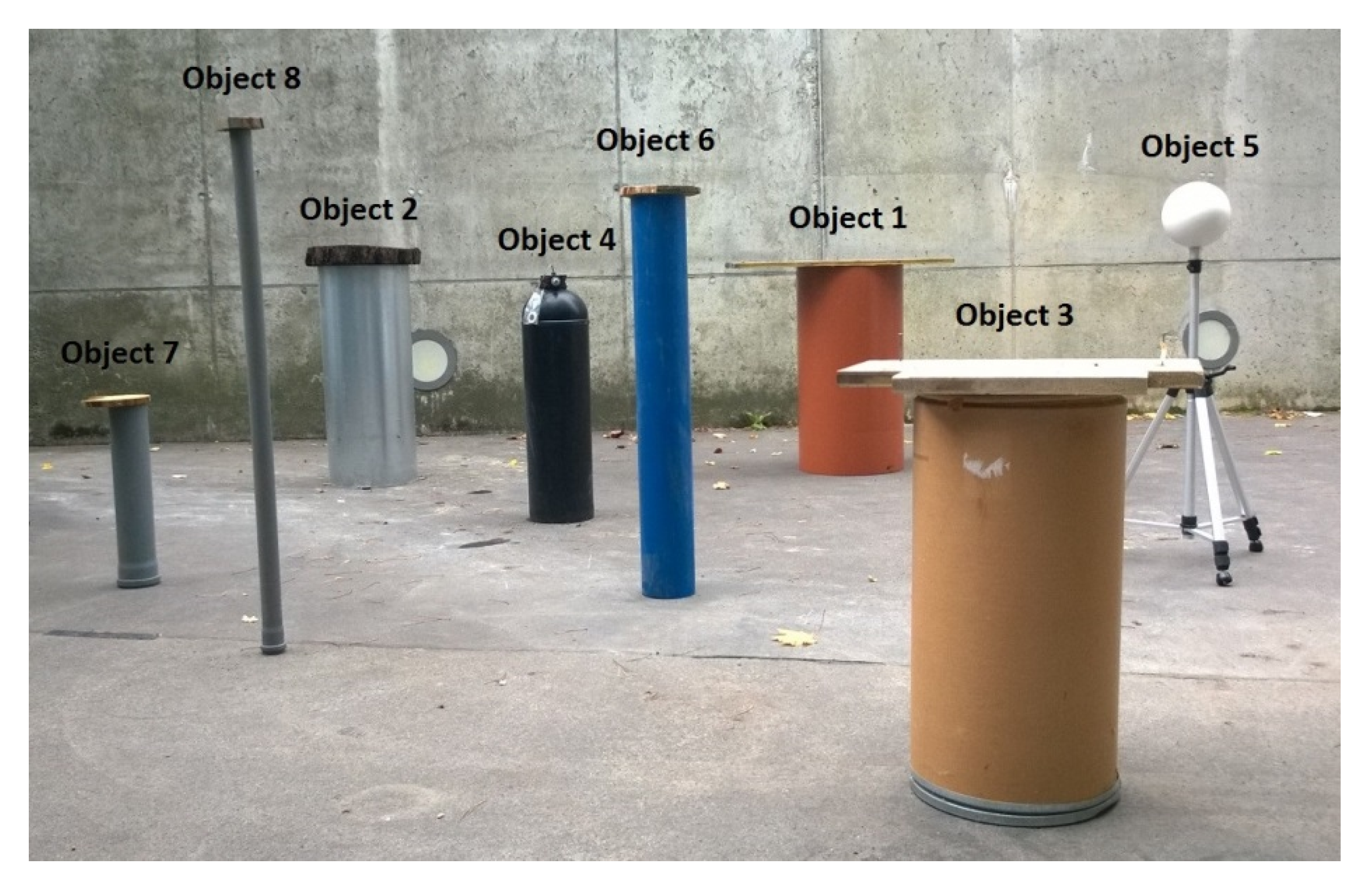
2.5. Evaluation of Point Cloud Quality and Diameter Fitting on Cylindrical Reference Objects

As the ZEB HORIZON PLS was new on the market at the time of the study, the quality of the point clouds and the performance of the diameter estimation algorithm were examined on seven cylindrical objects and one spherical object (Figure 3). In addition, a possible bias of the diameter estimation was also examined on the reference objects in order to eliminate the effects of tree species or bark. These objects were scanned under virtually perfect conditions (i.e., no wind, feature-rich environment, short scanning range, and high scanning resolution) to exclude disturbing effects from the forest environment and to judge the potential accuracy of the scanner. An overview of the objects, in terms of shape, material, and diameter, can be found in

Table 2. Overview of the objects in terms of shape, material, and diameter.

	Shape	Material	Diameter (cm)
Object 1	cylinder	plastic	49.8
Object 2	cylinder	metal	40.0
Object 3	cylinder	cardboard	36.1
Object 4	cylinder	plastic	25.5
Object 5	sphere	plastic	20.2
Object 6	cylinder	plastic	15.9
Object 7	cylinder	plastic	11.0
Object 8	cylinder	plastic	5.0

. All objects were cylindrically shaped, except for object 5 (Faro reference sphere). The surfaces of the objects were smooth and made of plastic (objects 1, 4–8), metal (object 2), or cardboard (object 3). The diameters of the objects were measured with a caliper, and were between 5 cm and 49.8 cm. The objects were scanned with the PLS in two scan surveys, with different walking speeds and using the same walk path with the same start and end point. Scanning times were 2 min and 1 min, respectively. In addition, the same objects were scanned from three scanning positions with the FARO Focus3D X330 TLS. For both PLS and TLS, care was taken to ensure that the objects received laser beams from all sides and the objects were covered to ensure that no laser beams hit the inside of the objects. PLS and TLS data were co-registered and exported with use of GeoSLAM Hub 5.2.0 software [74] and FARO SCENE 6.2 software [76], respectively. All parameter settings for the scanners and the software were the same as described in Section 2.2 and Section 2.3.

The individual objects were manually clipped out from the exported point clouds with the CloudCompare v2.10.2 software [105] and saved in LAS file format [75]. For these individual object point clouds, the diameters $d_{gam}$ and $d_{circ2}$ were then estimated at the half of the height, according to the methods described in Section 2.4 (Clustering, Detection of Tree Positions, and dbh Measurement). The deviation $\delta$ of the fitted diameters $\widehat{d}$ to the reference diameters $d$ was calculated as

$$\delta =\widehat{d}-d.$$

(1)

In addition, the standard deviation of the residuals from $d_{gam}$ ($s{d}_{res\_gam}$) was calculated and used as a measure of the noise in the point cloud. With the help of the intensity parameter, which was available for each individual 3D point, an average intensity of the layer was calculated. Then, $\delta$, $s{d}_{res\_gam}$, and average intensity were compared for each object between PLS (scan 1 and scan 2) and TLS.

2.6. Reference Data

Reference data for the actual dbh values and tree positions were derived from field data in March 2019. Based on a preliminary stem map of a study by Gollob et al. [20], trees were recorded if their dbh (measured from one direction with caliper in 1.3 m height) was greater than or equal to a lower threshold of 5 cm and if their distance from the sample plot center was 20 m or less. New trees that were not included in the preliminary stem map were recorded by measuring angles and distances to two known tree positions. To account for possible deviations from the north direction and to ensure that the estimated position and the reference position coordinates would be equal, an affine transformation of the found tree positions was carried out, with the help of 15 trees per sample plot, which were found by the algorithm and were also present in the reference data. This transformation was automatically performed using the function AffineTransformation() in the R package vec2dtransf [106]. The final assignment of tree positions was done using the function pppdist() in the R package spatstat [104]. This function performs a mapping of two similar point patterns by minimizing the average Euclidean distance between matching points. Automatically detected tree positions which could not be assigned to a tree measured in the reference data were manually double-checked in the TLS point cloud. Depending on the results of the check, either the automatically detected tree position was marked as a false positive or, in the case where the tree was visible in the point cloud but missing during the reference measurements in the field, the co-ordinates were added to the reference data post-hoc.

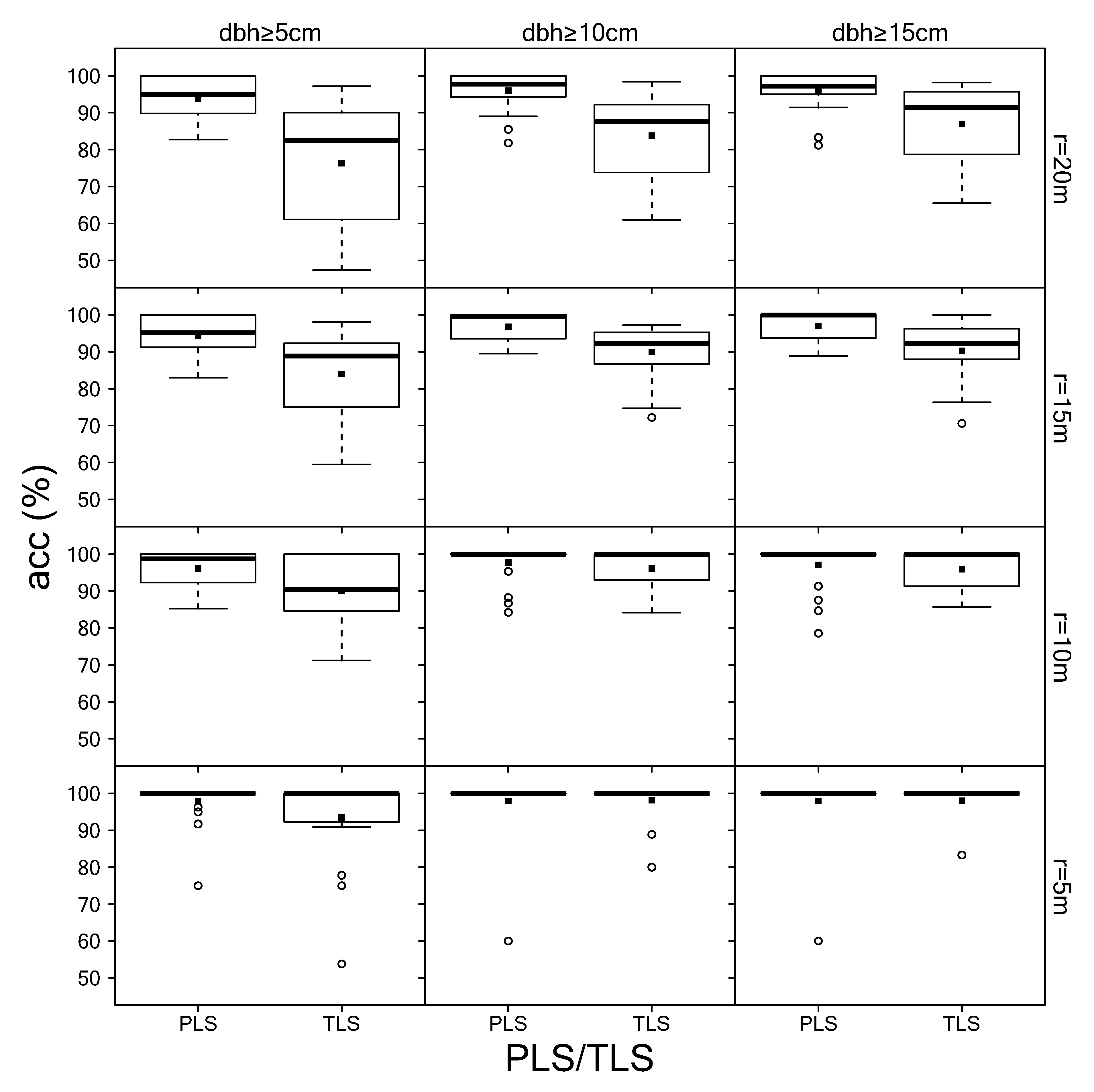
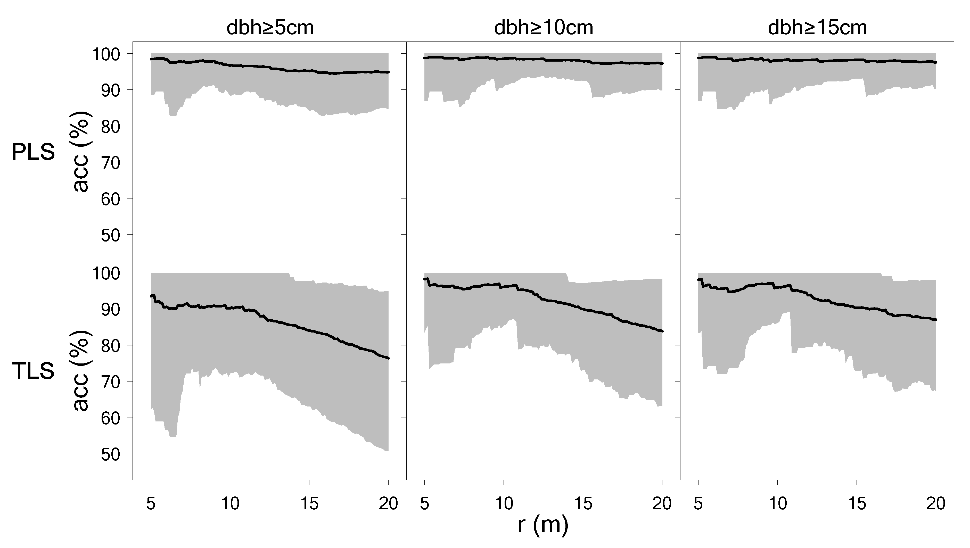
2.7. Accuracy of Tree Detection and dbh Measurement

The accuracy of tree detection was evaluated in terms of three measures: detection rate $d_r(\%)$, commission error $c(\%)$, and overall accuracy $acc(\%)$. These measures were calculated as follows:

$$d_r(\%)=\frac{n_{\mathrm{match}}}{n_{\mathrm{ref}}}\times 100,$$

(2)

$$c(\%)=\frac{n_{\mathrm{falsepos}}}{n_{\mathrm{extr}}}\times 100,$$

(3)

$$acc(\%)=100\%-\left(o(\%)+c(\%)\right),$$

(4)

where $n_{\mathrm{match}}$ is the number of correctly found reference trees; $n_{\mathrm{ref}}$ is the total number of reference trees; $n_{\mathrm{falsepos}}$ is the number of tree positions which could not be assigned to an existing tree in the reference data; $n_{\mathrm{extr}}$ is the number of automatically detected tree positions ($n_{\mathrm{match}}+n_{\mathrm{falsepos}}$); and $o(\%)$ is the omission error, defined as $100\%-d_r(\%)$. The detection rate $d_r (\%)$ measures the proportion of correctly detected tree locations, the commission error $c (\%)$ measures the proportion of falsely detected tree locations, and the overall accuracy $acc(\%)$ is a combination of the latter two metrics and represents a global quality criterion.

The accuracy of the automatic dbh measurements was assessed by means of root mean square error (RMSE), calculated as the square root of the average quadratic deviation between the automatic measurement ${\widehat{dbh}}_i$ and the corresponding reference measurement $db{h}_i$:

$$\mathrm{RMSE}=\sqrt{\frac{1}{n_{\mathrm{match}}}{{\displaystyle \sum }}_{i=1}^{n_{\mathrm{match}}}{\left({\widehat{dbh}}_i-db{h}_i\right)}^2}.$$

(5)

The precision of the automatic dbh measurements was assessed in terms of bias:

$$\mathrm{bias}=\frac{1}{n_{\mathrm{match}}}{{\displaystyle \sum }}_{i=1}^{n_{\mathrm{match}}}\left({\widehat{dbh}}_i-db{h}_i\right).$$

(6)

The deviation between the automatic measurement ${\widehat{dbh}}_i$ and the corresponding reference measurement $db{h}_i$ was computed analogously to Equation (1), and is referred to as ${\delta }_{dbh}$.

RMSE and bias were also calculated as relative measures (RMSE% and bias%):

$$\mathrm{RMSE}\%=\frac{\mathrm{RMSE}}{\overline{dbh}}\times 100,$$

(7)

$$\mathrm{bias}\%=\frac{\mathrm{bias}}{\overline{dbh}}\times 100,$$

(8)

with

$$\overline{dbh}=\frac{1}{n_{\mathrm{match}}}{{\displaystyle \sum }}_{i=1}^{n_{\mathrm{match}}}db{h}_i$$

(9)

being the average dbh of the reference data.

In order to examine whether, and to what extent, the accuracy of the automatic tree detection was influenced by the distance of a tree from the sample plot center, the performance measures for tree detection described above were separately assessed for four subplot sizes defined by disks with radii of 20 m, 15 m, 10 m, and 5 m. In addition, it was analyzed whether the performance of the automatic routines showed trends depending on the size of the trees. For this purpose, the performance measures were evaluated for subsets defined by the three lower dbh thresholds of 5 cm, 10 cm, and 15 cm. Furthermore, the performance of tree detection of PLS and TLS was compared with regard to the lower dbh thresholds and various plot sizes. The deviations δ_i of the estimated dbh values from the reference diameters were analyzed for the different tree species.

To investigate the possible influence of scanner noise and dbh on ${\delta }_i$, a simulation study was performed. For every dbh between 1 cm and 20 cm (with step size 0.5 cm), 1000 cross-sections were simulated. For every cross-section, a noisy point cloud was simulated in polar co-ordinates by adding a normally distributed random error to 1000 radii that were evenly distributed over 1000 angles ranging from -π to π. The random error had a mean of 0 cm and different standard deviations (1 cm, 2 cm, 2.45 cm, and 3 cm), in order to account for different levels of unbiased noise. The standard deviation of 2.45 cm is the mean $s{d}_{res\_gam}$ for all $d_{gam}$ in PLS data. Then, the simulated point cloud was transformed into Cartesian coordinates, and the diameters $d_{gam}$ and $d_{circ2}$ were fitted to assess possible model bias.

In order to correct the estimated PLS diameters for a possible dbh-related bias, the dbh deviation ${\delta }_{dbh}$ was modeled using a simple linear model. For practicality, the proposed linear model should include variables which are easy to estimate accurately, either in the field or during processing. We used the following linear model for bias correction:

$$\begin{gathered} \widehat{{\delta }_{dbh}} ={\beta }_0+{\beta }_1\times \log (d_{gam})+{\beta }_2\times mea{n}_{inten}+{\beta }_3\times s{d}_{re{s}_{gam}}+{\beta }_4 \\ \times \left(mea{n}_{inten}\times s{d}_{re{s}_{gam}}\right)+ϵ, \end{gathered}$$

(10)

where $\widehat{{\delta }_{dbh}}$ is the dbh deviation, log($d_{gam}$) is the logarithmic natural cubic spline dbh, $mean\_inten$ is the mean intensity of the cross-section 3D points, $s{d}_{res\_gam}$ is the standard deviation of the spline residuals, $mean\_inten\times s{d}_{res\_gam}$ is an interaction term, $ϵ$ is the residual error, and ${\beta }_0, \dots , {\beta }_4$ are linear coefficients.

To evaluate the significant effects of the above-mentioned covariates, a linear regression model was formulated using the lm() function in R. Before that, the predictor variables were plotted against the dependent variable and, in the course of modeling, any plausible interactions were also tested.

In order to determine the necessary sample size for modeling the dbh-related bias with satisfactory precision, we performed cross-validations with sample sizes varying between 30 and 500 for the model data set; that is, we investigated how many dbhs have to be measured manually in order to obtain robust predictions for the remaining dbh deviations. For each sample size, 10,000 random samples of the reference dbh values were drawn. Then, the $\widehat{{\delta }_{dbh}}$ were predicted on the independent validation sets. The dbh-related bias of $d_{gam}$ was then corrected by $\widehat{{\delta }_{dbh}}$ and, as a quality criterion, the RMSE was calculated. The deviations ${\delta }_{dbh}$ of the corrected estimated diameters $d_{gam\_corr}$ were analyzed in relationship with the reference diameters.

3. Results

3.1. Detection of Tree Positions

The analysis of the sample plots (20 for PLS, 17 for TLS) showed that the detection rate $d_r(\%)$ strongly depended on the lower dbh threshold and the sample plot radius applied as a maximum radius (Figure 4). In general, the detection rate increased with an increasing lower threshold for dbh and a decreasing maximum radius. Furthermore, it can be seen that TLS scans generally had lower detection rates, which became more pronounced with a lower threshold for dbh and an increasing sample plot radius. The range of the detection rates in the sample plots were always smaller with PLS than with TLS. The average detection rates for PLS over all 20 sample plots, dbh thresholds, and plot radii ranged from 95.99% to 100%, while the corresponding average detection rates for TLS on 17 plots ranged from 78.46% to 99.02%. Using plot radii of 20 m, 15 m, and 10 m, and a lower dbh threshold of 10 cm, the respective average detection rates for PLS were 98.76%, 98.95%, and 99.48%, while the respective values for TLS were 86.32%, 93.81%, and 98.35% (see further details in Appendix B,

Table A3. Detection rates, commission errors, and overall accuracies for PLS/TLS, lower dbh thresholds, and plot radii.

		$\mathbf{Detection} \mathbf{Rate} {\mathit{d}}_{\mathit{r}}\left(\mathit{\%}\right)$		$\mathbf{Commission} \mathbf{Error} \mathit{c} \left(\mathit{\%}\right)$		$\mathbf{Overall} \mathbf{Accuracy} \mathit{a}\mathit{c}\mathit{c} \left(\mathit{\%}\right)$
Radius	dbh	PLS	TLS	PLS	TLS	PLS	TLS
20 m	≥5 cm	95.99	78.46	1.13	2.41	94.83	76.38
20 m	≥10 cm	98.76	86.32	1.40	2.70	97.29	83.81
20 m	≥15 cm	99.36	90.07	1.69	3.19	97.58	87.04
15 m	≥5 cm	95.98	87.33	0.84	3.26	95.16	84.05
15 m	≥10 cm	98.95	93.81	1.06	3.68	97.86	89.96
15 m	≥15 cm	99.56	94.78	1.29	4.27	98.24	90.33
10 m	≥5 cm	97.33	92.22	0.66	1.98	96.67	90.15
10 m	≥10 cm	99.48	98.35	0.91	2.08	98.55	96.08
10 m	≥15 cm	99.18	98.64	1.08	2.47	98.05	95.93
5 m	≥5 cm	99.15	93.97	0.62	0.42	98.44	93.52
5 m	≥10 cm	100.00	98.82	1.00	0.59	98.75	98.17
5 m	≥15 cm	100.00	99.02	1.00	0.84	98.75	98.04

). Using a lower dbh threshold of 10 cm and plot radii of 20 m, 15 m, and 10 m, a respective detection rate of 100% was achieved on 90%, 70%, and 60% of the sample plots using PLS, while it was only achieved on 76%, 35%, and 6% of the sample plots using TLS.

The commission error (Figure 5) increased with increasing lower dbh threshold and maximum radius. This increase was more obvious with TLS than with PLS. The commission error differed only slightly among dbh threshold and maximum radii for PLS. In general, the average and the range of the commission errors were smaller with PLS than with TLS. The average commission errors for PLS over all 20 sample plots, dbh thresholds, and plot radii ranged from 0.62% to 1.69%, while the corresponding average commission errors for TLS on 17 plots ranged from 0.42% to 4.27%.

Overall accuracy rates ($acc(\%)$), as a combination of detection and commission rates, are presented in Figure 6. Overall accuracy showed similar behavior to detection rate, depending on dbh threshold, plot radius, and scan variant. Average overall accuracies for PLS across all 20 sample plots varied between 94.83% and 98.75%, while the average overall accuracies for TLS on 17 plots varied between 76.38% and 98.17%. Using plot radii of 20 m, 15 m, and 10 m, and a lower dbh threshold of 10 cm, respective average overall accuracies for PLS were 97.29%, 97.86%, and 98.55%. The respective values for TLS were 83.81%, 89.96%, and 96.08% (see further details in Appendix B, Table A3).

Using a lower dbh threshold of 10 cm and plot radii of 20 m, 15 m, and 10 m, a respective overall accuracy of 100% was achieved on 80%, 50%, and 40% of the sample plots using PLS, while it was only achieved on 59%, 0%, and 0% of the sample plots using TLS.

The performance in terms of tree detection separately for each sample plot can be found in Appendix B, Table A3.

The relationship between overall accuracy and maximum sample plot radius was analyzed, in more detail, for PLS and TLS. The curves of the overall accuracy rates over the sample plot radii had a similar shape for all three lower dbh thresholds (Figure 7). However, the level of the curve (i.e., the overall accuracy) was lowest for the 5 cm threshold and highest for the 15 cm threshold. Furthermore, it can be seen that the overall accuracies of PLS decreased only slightly with increasing sample plot radii. In comparison, the overall accuracies of TLS remained almost constant, up to a sample plot radius of approx. 10 m, and continuously declined for sample plot radii greater than 10 m.

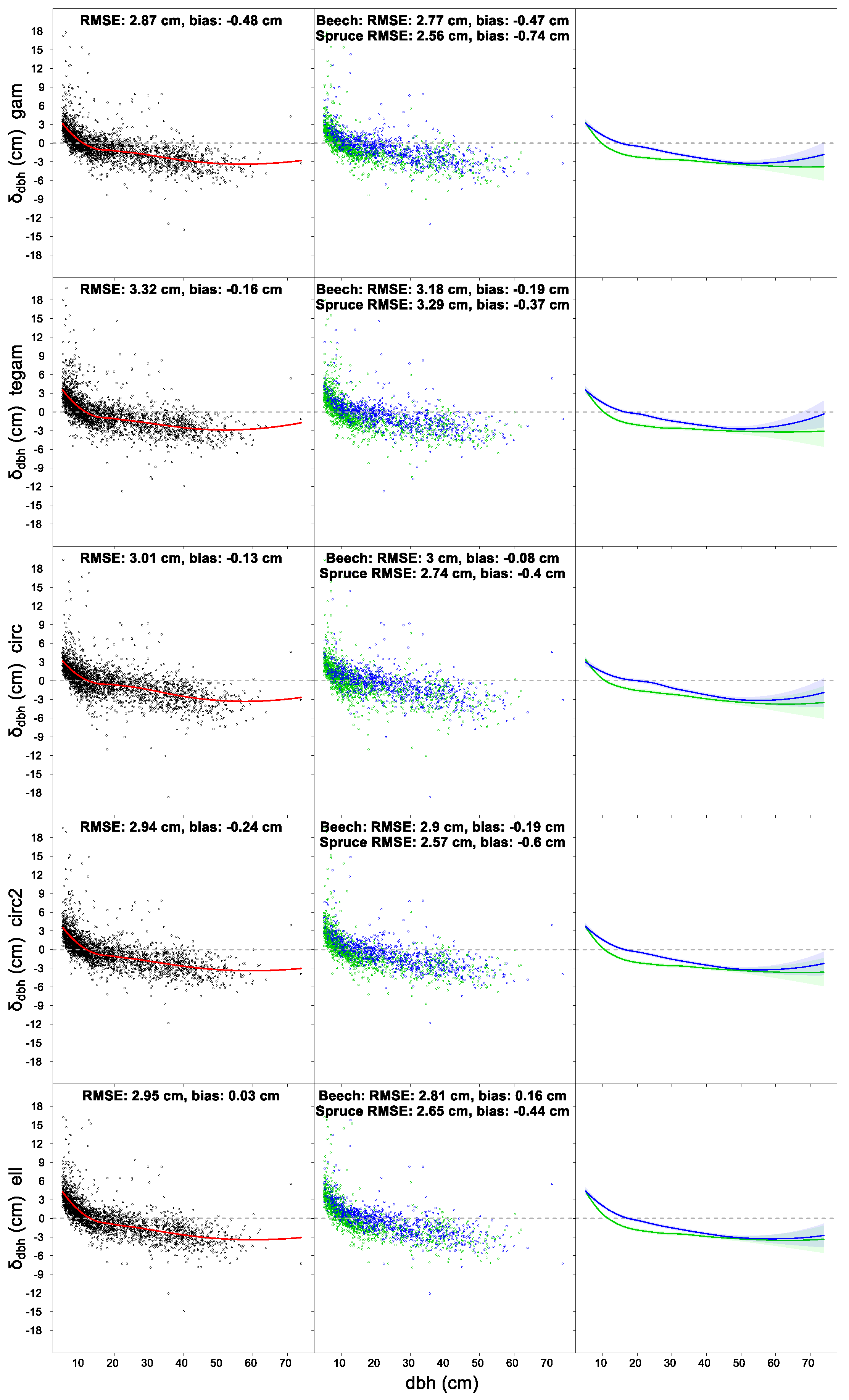
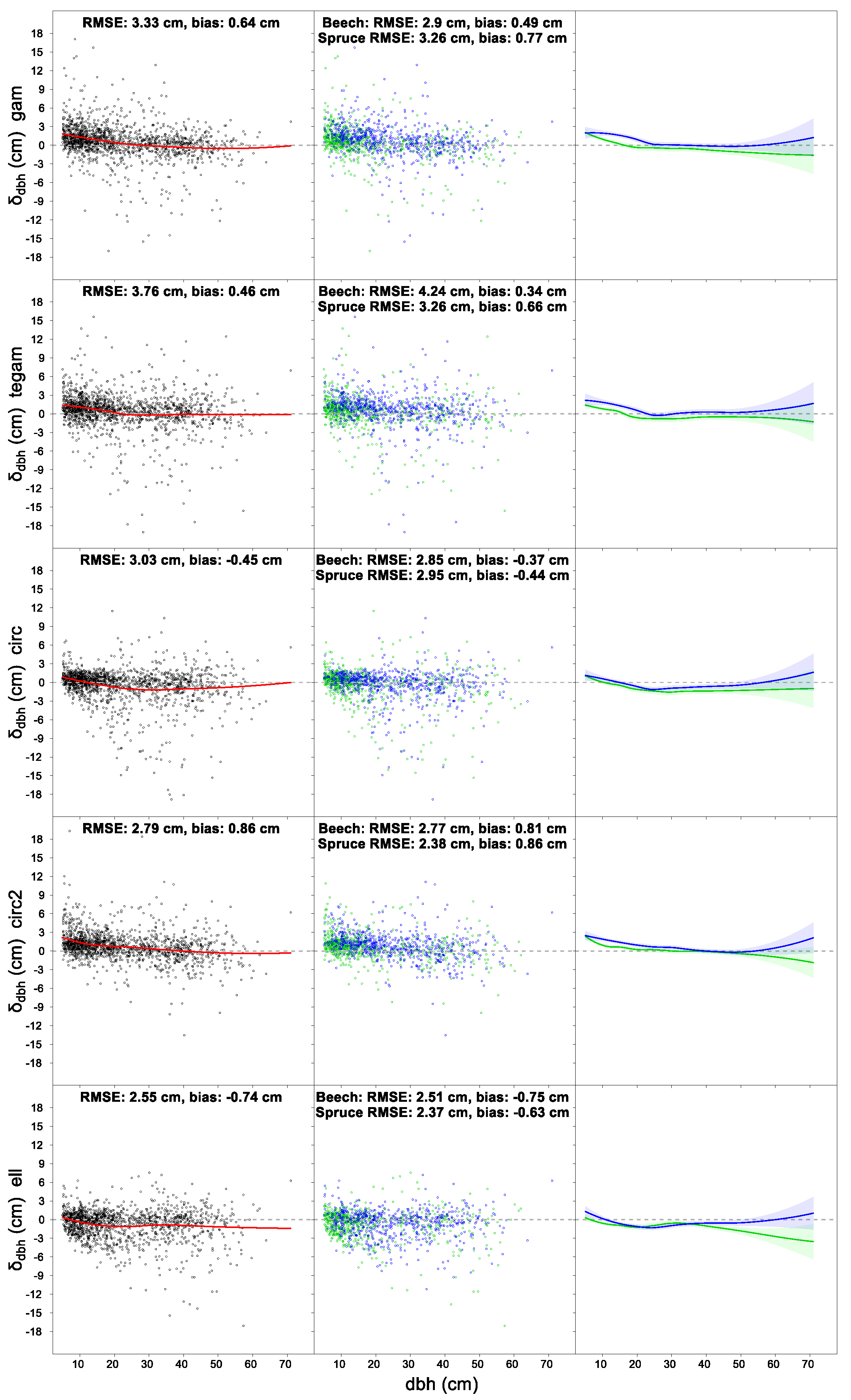
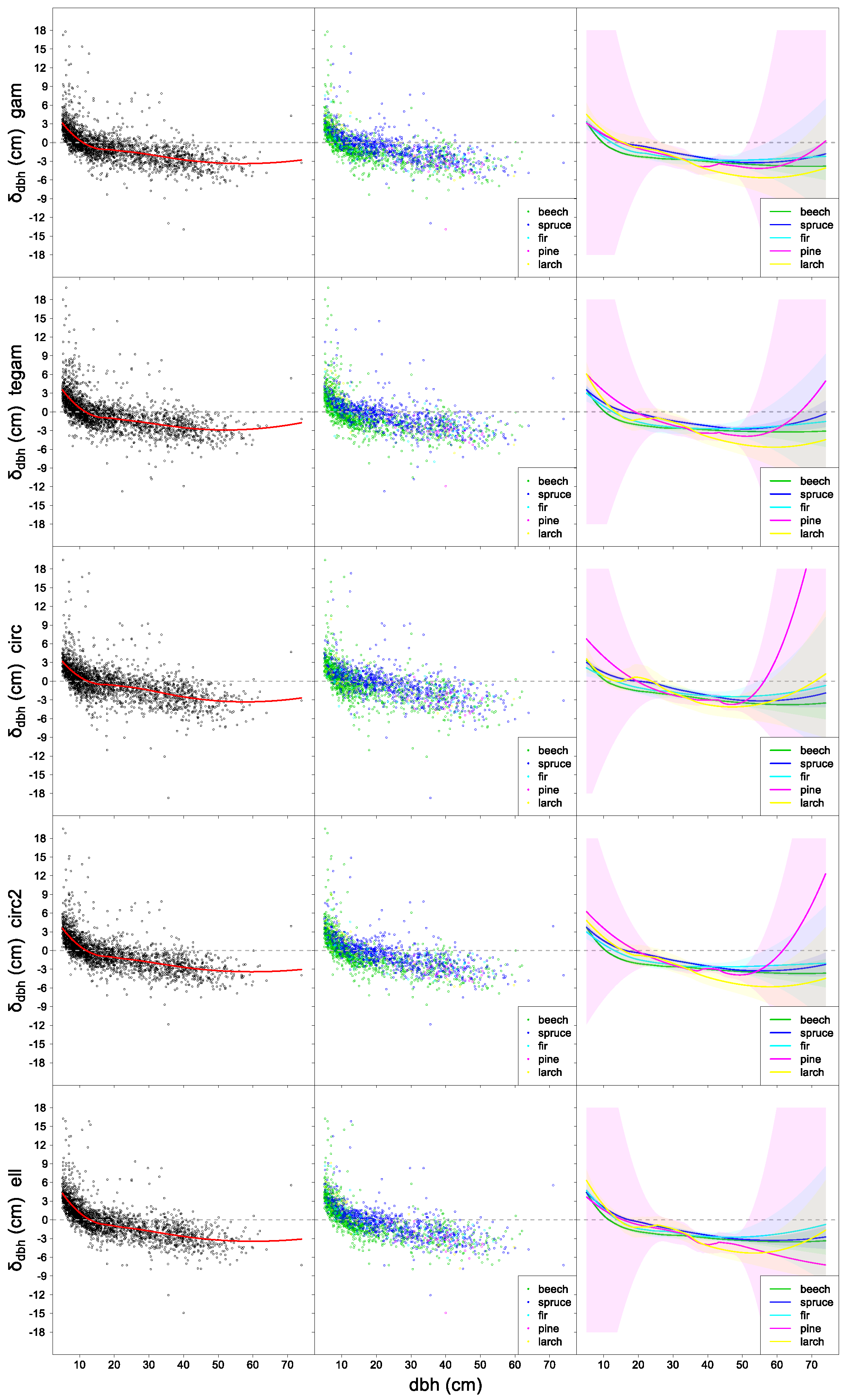
3.2. Estimation of dbh

3.2.1. Personal Laser Scanning (PLS)

The performance of automatic dbh estimation, in terms of deviation between dbh estimates from PLS and dbh measured in the field, is outlined in Figure 8. For all dbh fitting methods (i.e., $d_{gam}$, $d_{tegam}$, $d_{circ}$, $d_{circ}$, $d_{circ2}$, and $d_{ell}$), small diameters (dbh < 10 cm) were generally overestimated, while large diameters (dbh > 10 cm) were generally underestimated. Underestimation increased with further increasing dbh, and the overestimation increased with decreasing dbh. Evaluating the various dbh fitting methods, the RMSE ranged between 2.87 cm (14.85%) and 3.32 cm (17.18%) and the bias between −0.48 cm (−2.48%) and 0.03 cm (0.16%). The lowest RMSE was obtained by $d_{gam}$ (2.87 cm = 14.85%), while the lowest bias was obtained by $d_{ell}$ (0.03 cm = 0.16%). The mean standard deviation ($s{d}_{res\_gam}$) of the residuals from $d_{gam}$ was 2.45 cm, which can be considered as measure for the noise in the PLS point cloud. A separate representation of spruce and beech showed that there were discernible differences between the tree species. In the case of beech, the RMSE ranged between 2.77 cm (16.32%) and 3.18 cm (19.49%) and the bias between −0.47 cm (−2.88%) and 0.16 cm (0.98%). For spruce, the RMSE ranged between 2.56 cm (10.62%) and 3.29 cm (13.46%) and the bias between −0.74 cm (−3.07%) and −0.40 cm (−1.66%). For an overview of the dbh deviations for all tree species, refer to Appendix C, Figure A2. The performance of dbh estimation separately for each sample plot is presented in Appendix B,

Table A4. Performance of tree detection and diameter estimation for PLS/TLS with a lower dbh threshold of 5 cm and plot radius of 20 m.

Plot	${\mathit{d}}_{\mathit{r}}\left(\mathit{\%}\right) \mathbf{PLS}$	${\mathit{d}}_{\mathit{r}}\left(\mathit{\%}\right) \mathbf{TLS}$	$\mathit{c} \left(\mathit{\%}\right) \mathbf{PLS}$	$\mathit{c} \left(\mathit{\%}\right) \mathbf{TLS}$	$\mathit{a}\mathit{c}\mathit{c} \left(\mathit{\%}\right) \mathbf{PLS}$	$\mathit{a}\mathit{c}\mathit{c} \left(\mathit{\%}\right) \mathbf{TLS}$	$\mathit{R}\mathit{M}\mathit{S}\mathit{E} \left(\mathbf{cm}\right) \mathbf{PLS}$	$\mathit{R}\mathit{M}\mathit{S}\mathit{E} \left(\mathbf{cm}\right) \mathbf{TLS}$	$\mathit{R}\mathit{M}\mathit{S}\mathit{E} \mathbf{corr}. \left(\mathbf{cm}\right) \mathbf{PLS}$	$\mathit{b}\mathit{i}\mathit{a}\mathit{s} \left(\mathbf{cm}\right) \mathbf{PLS}$	$\mathit{b}\mathit{i}\mathit{a}\mathit{s} \left(\mathbf{cm}\right) \mathbf{TLS}$	$\mathit{b}\mathit{i}\mathit{a}\mathit{s} \mathbf{corr}. \left(\mathbf{cm}\right) \mathbf{PLS}$	$\mathit{s}{\mathit{d}}_{\mathit{r}\mathit{e}\mathit{s}\_\mathit{g}\mathit{a}\mathit{m} } \left(\mathbf{cm}\right) \mathbf{PLS}$	$\mathit{s}{\mathit{d}}_{\mathit{r}\mathit{e}\mathit{s}\_\mathit{g}\mathit{a}\mathit{m} } \left(\mathbf{cm}\right) \mathbf{TLS}$	Time (min) PLS	Time (min) TLS
1	100.0	91.7	0.0	1.1	100.0	90.6	2.96	2.38	2.11	−1.32	−0.75	−0.92	2.58	0.55	9.1	49.6
2	100.0		0.0		100.0		1.95		1.64	−1.06		0.49	2.58		7.3
3	100.0	93.3	0.0	3.4	100.0	90.0	3.79	5.11	2.50	−3.59	−2.40	−1.93	2.78	0.58	11.7	49.6
4	95.0	78.8	1.3	0.0	93.8	78.8	3.56	1.67	2.02	−0.23	−0.24	0.09	2.55	0.54	12.0	49.6
5	90.8	63.8	0.4	1.1	90.5	63.1	2.79	2.89	2.51	0.22	−1.11	−0.35	2.43	0.62	13.4	49.6
6	83.3	47.3	0.4	0.0	82.9	47.3	3.50	2.16	3.16	0.52	−0.88	0.29	2.33	0.56	10.7	49.6
7	100.0	69.4	7.7	10.7	91.7	61.1	3.15	4.20	2.44	−2.35	−2.30	−0.98	2.69	0.46	13.9	49.6
8	97.4	62.9	1.3	3.1	96.0	60.9	4.00	2.50	3.81	0.86	−1.21	1.55	2.57	0.58	13.5	49.6
9	92.2	56.1	0.0	0.4	92.2	55.9	1.83	2.28	1.98	0.21	−0.55	0.80	2.18	0.57	15.5	49.6
10	95.2	92.9	0.0	1.5	95.2	91.4	3.67	2.06	2.51	−2.13	0.34	−1.21	2.74	0.50	8.5	49.6
11	100.0	90.0	0.0	2.2	100.0	88.0	3.13	3.54	2.66	−1.92	−1.21	0.91	2.67	0.47	11.4	49.6
12	98.2	93.4	1.8	5.0	96.4	88.5	3.26	1.52	1.67	−2.63	−0.27	−0.03	2.61	0.39	10.6	49.6
13	90.6	72.3	0.7	0.0	89.9	72.3	3.27	2.34	2.86	−0.41	−0.91	0.80	2.50	0.61	13.1	49.6
14	100.0	97.2	0.0	0.0	100.0	97.2	2.26	1.86	1.47	−1.37	−0.21	0.34	2.59	0.39	8.6	49.6
15	87.3	57.1	0.7	0.9	86.7	56.6	2.25	3.19	2.10	−0.2	−1.06	0.54	2.52	0.61	10.6	49.6
16	100.0	94.4	0.0	4.2	100.0	90.3	3.17	2.39	1.61	−2.05	−0.84	0.00	2.70	0.55	12.1	49.6
17	95.2	88.7	6.3	5.2	88.7	83.9	2.62	1.91	1.50	−1.91	−0.18	0.51	2.58	0.41	9.8	49.6
18	99.0	84.5	2.0	2.2	97.0	82.5	2.97	2.59	1.81	−1.81	−0.21	−0.10	2.45	0.44	11.0	49.6
19	97.9		0.0		97.9		2.29		1.95	−0.46		0.02	2.39		8.0
20	97.7		0.0		97.7		2.01		1.59	−0.53		−0.48	2.35		8.3

.

3.2.2. Terrestrial Laser Scanning (TLS)

The performance of automatic dbh estimation, in terms of deviation between dbh estimates from TLS and dbh measured in the field, is outlined in Figure 9. For some dbh fitting methods ($d_{gam}$, $d_{tegam}$, $d_{circ}$, and $d_{circ2}$), small diameters (dbh < 10 cm) were overestimated. Large diameters (dbh > 10 cm) were underestimated for $d_{circ}$ and $d_{gam}$. Evaluating the various dbh fitting methods, the RMSE ranged between 2.55 cm (13.19%) and 3.32 cm (19.45%) and the bias between −0.74 cm (−3.83%) and 0.86 cm (4.45%). The lowest RMSE was obtained by $d_{ell}$ (2.55 cm = 13.19%), while the lowest bias was obtained by $d_{circ}$ (−0.45 cm = −2.33%). The mean standard deviation of the residuals from $d_{gam}$ was 0.52 cm, which can be considered as measure of the noise in the TLS point cloud. A separate representation of spruce and beech showed that there were no discernible differences between the tree species. In the case of beech, the RMSE ranged between 2.51 cm (15.38%) and 4.24 cm (25.98%) and the bias between −0.75 cm (−4.60%) and 0.81 cm (4.96%). For spruce, the RMSE ranged between 2.37 cm (9.83%) and 3.26 cm (13.52%) and the bias between −0.63 cm (−2.61%) and 0.86 cm (3.57%). The performance of dbh estimation separately for each sample plot is presented in Appendix B, Table A4.

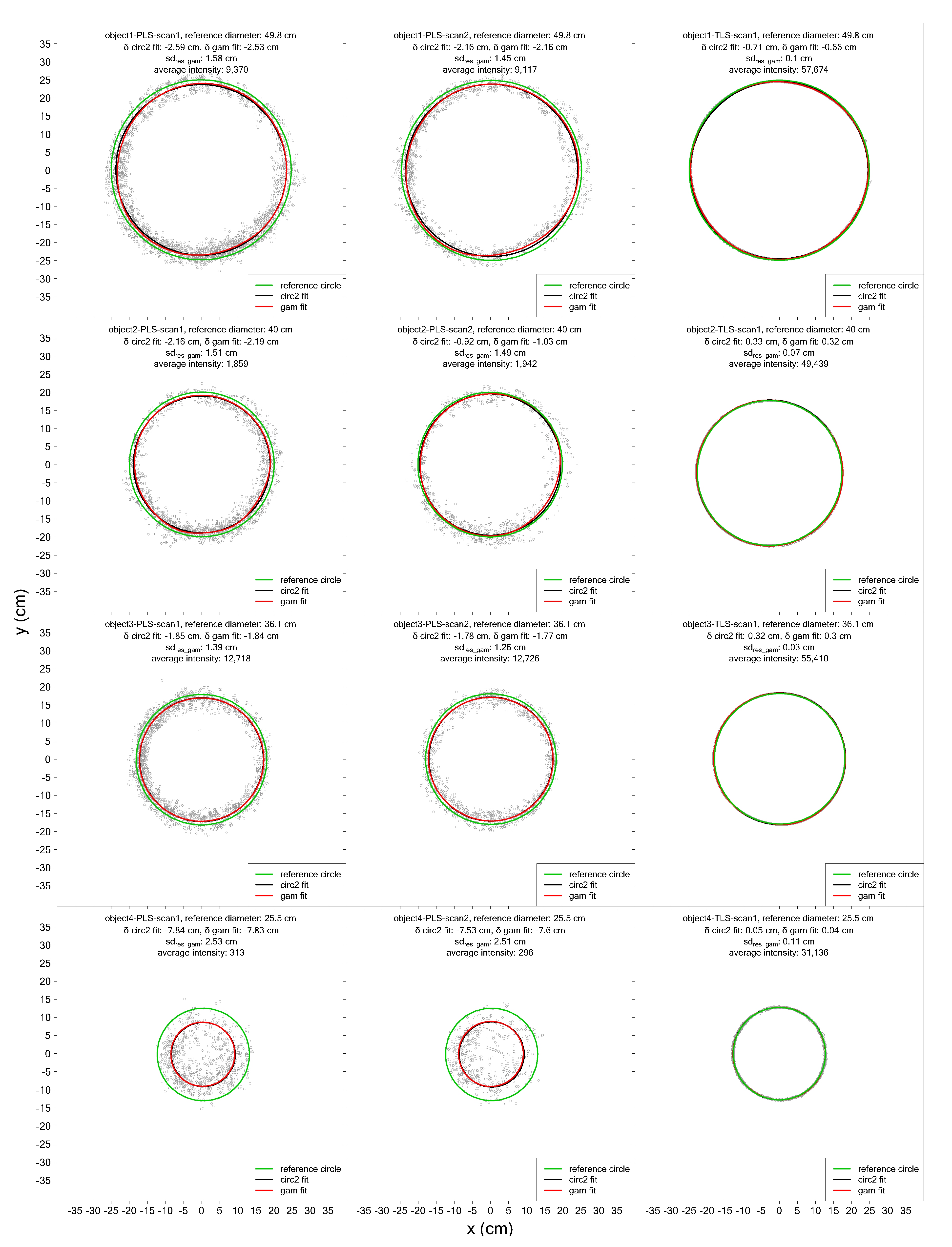
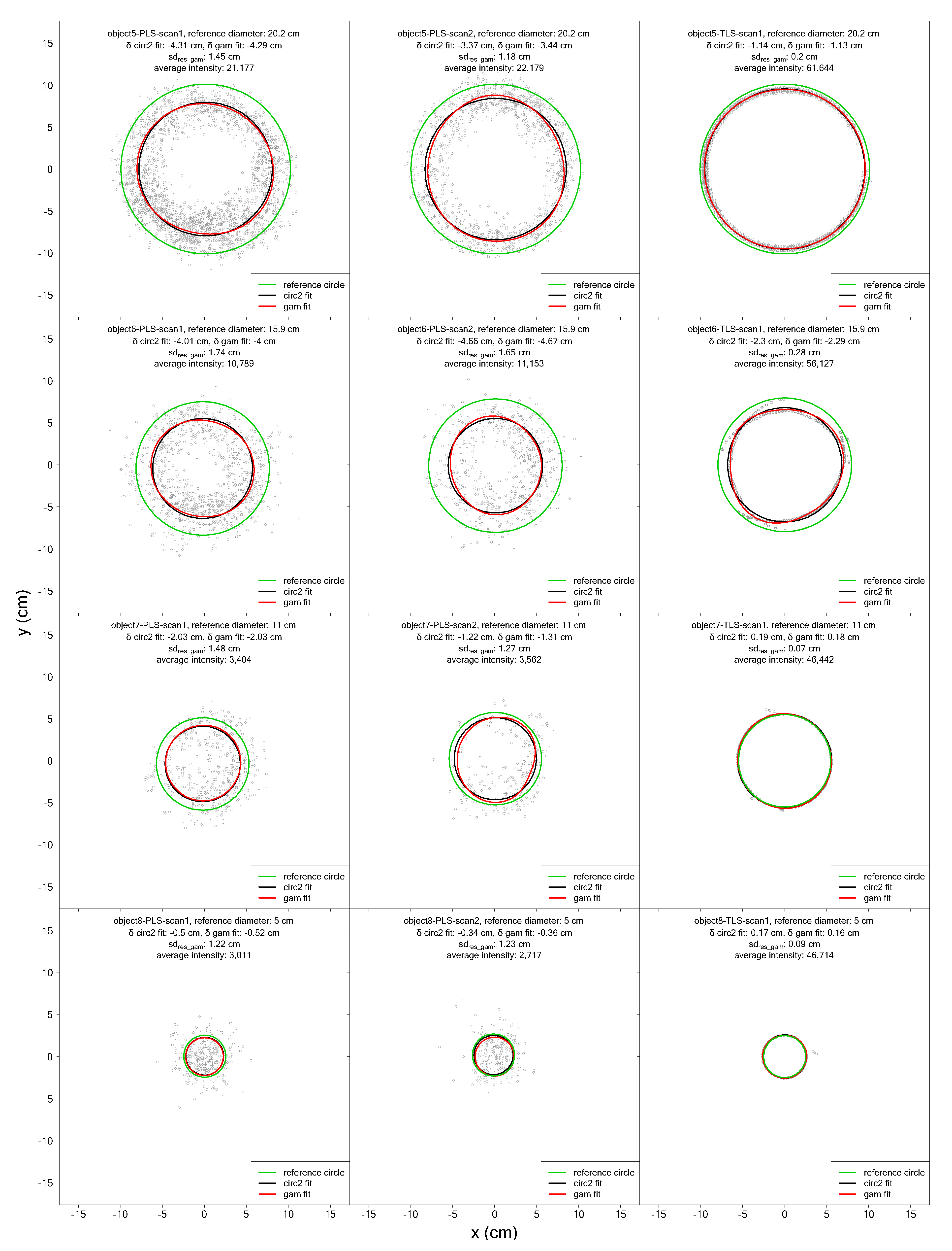
3.3. Cylindrical Reference Objects under Controlled Conditions

For a better understanding of the performance of PLS with regard to dbh measurement, and to better evaluate the dbh results obtained with PLS in the forest, reference data were collected on eight objects under perfect scanning conditions. For the individual object point clouds, the diameters $d_{gam}$ and $d_{circ2}$ were estimated using the same algorithms for diameter estimation as in the forest. The evaluation of two PLS scans (scan 1: 2 min and scan 2: 1 min) and a TLS scan with regard to diameter deviation $\delta$, standard deviation of the residuals from the natural cubic spline $s{d}_{res\_gam}$, and average intensity of the points belonging to the cross-section can be found in

Table 3. Evaluation of PLS and TLS on cylindrical reference objects.

Object	Reference Diameter (cm)	PLS Scan 1				PLS Scan 2				TLS Scan 1
		Scan Time: 2 min				Scan Time: 1 min				Scan Time: 27 min
		$\mathit{\delta }$	$\mathit{\delta }$	$\mathit{s}{\mathit{d}}_{\mathit{r}\mathit{e}\mathit{s}\_\mathit{g}\mathit{a}\mathit{m} } \left(\mathbf{cm}\right)$	Aver-Age Inten-Sity	$\mathit{\delta }$	$\mathit{\delta }$	$\mathit{s}{\mathit{d}}_{\mathit{r}\mathit{e}\mathit{s}\_\mathit{g}\mathit{a}\mathit{m} } \left(\mathbf{cm}\right)$	Aver-Age Inten-Sity	$\mathit{\delta }$	$\mathit{\delta }$	$\mathit{s}{\mathit{d}}_{\mathit{r}\mathit{e}\mathit{s}\_\mathit{g}\mathit{a}\mathit{m} } \left(\mathbf{cm}\right)$	Aver-Age Inten-Sity
Object 1	49.80	−2.59	−2.53	1.58	9370	−2.16	−2.16	1.45	9117	−0.71	−0.66	0.10	57,674
Object 2	40.00	−2.16	−2.19	1.51	1859	−0.92	−1.03	1.49	1942	0.33	0.32	0.07	49,439
Object 3	36.10	−1.85	−1.84	1.39	12,718	−1.78	−1.77	1.26	12,726	0.32	0.3	0.03	55,410
Object 4	25.50	−7.84	−7.83	2.53	313	−7.53	−7.60	2.51	296	0.05	0.04	0.11	31,136
Object 5	20.20	−4.31	−4.29	1.45	21,177	−3.37	−3.44	1.18	22,179	−1.14	−1.13	0.2	61,644
Object 6	15.90	−4.01	−4.00	1.74	10,789	−4.66	−4.67	1.65	11,153	−2.30	−2.29	0.28	56,127
Object 7	11.00	−2.03	−2.03	1.48	3404	−1.22	−1.31	1.27	3562	0.19	0.18	0.07	46.442
Object 8	5.00	−0.50	−0.52	1.22	3011	−0.34	−0.36	1.23	2717	0.17	0.16	0.09	46,714

. In general, it can be seen that the deviations from the reference diameter were higher with PLS than with TLS. Furthermore, the noise in the point clouds, as measured by the standard deviation of the residuals $s{d}_{res\_gam}$, was lower with TLS (0.03–0.28 cm) than with PLS (1.18–2.53 cm). The mean intensities were higher with TLS. The values of the deviations showed no relationship with the reference diameters. When comparing PLS scans 1 and 2, it was noticed that PLS scan 2 (with 1 min scan time) generally had lower diameter deviations and residual standard deviation. The highest PLS diameter deviation occurred with object 4 (scan 1: −7.84 cm, scan 2: −7.60 cm). Object 4 also had the highest noise, in terms of $s{d}_{res\_gam}$ (scan 1: 2.53 cm, scan 2: 2.51 cm), and the lowest average intensity (scan 1: 313, scan 2: 296). For TLS, object 6 had the highest deviation (−2.30 cm) with the highest noise in terms of $s{d}_{res\_gam}$. PLS scans 1 and 2 showed a systematic underestimation (scan 1: −0.50 to −7.84 cm, scan 2: −0.34 to −7.60 cm) of the diameters whereas, for TLS, both underestimation and overestimation (−2.30 cm to 0.33 cm) existed. A comparison of the diameter fitting methods showed that, with PLS scan 1 and TLS, $d_{gam}$ basically caused lower deviations and, with PLS scan 2, the opposite occurred. An overview of the eight object cross-sections, including the fitted diameters, deviations, standard deviations of the residuals, and average intensities, can be found in Appendix C, Figure A3 and Figure A4.

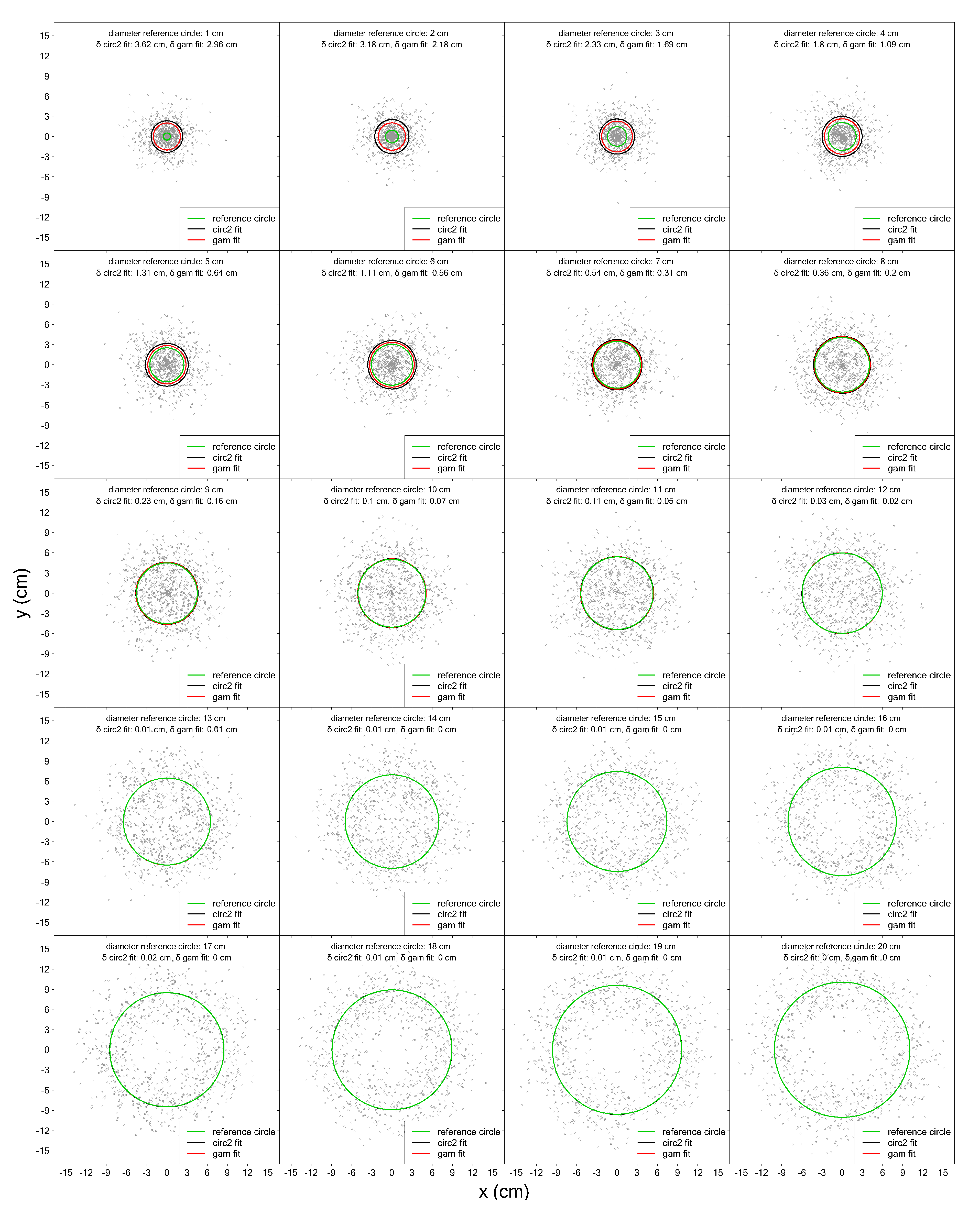
3.4. Simulated Noisy Cross-Sections

To explain the overestimation of the small trees, 1000 cross-sections, each with a dbh of 1–20 cm, were simulated. Normally distributed random errors with mean of 0 cm and standard deviations of 1 cm, 2 cm, 2.45 cm, and 3 cm were added to the distances (radii in a closed circle) of 1000 polar co-ordinates per tree to simulate noisy cross-sections. The transformation to Cartesian coordinates resulted in cross-sections, to which $d_{gam}$ and $d_{circ2}$ were fitted. The bias resulting from the comparison with the error-free diameters is presented in Figure 10. In general, the bias drastically increased with decreasing reference diameter. With increasing standard deviation, the bias occurred with larger reference diameters and, thus, bias became larger for a given diameter. With regard to the diameter fitting method, $d_{gam}$ caused a smaller bias than $d_{circ2}$. Simulated examples of noisy cross-sections with sd = 2.45 cm are presented in Appendix C, Figure A5.

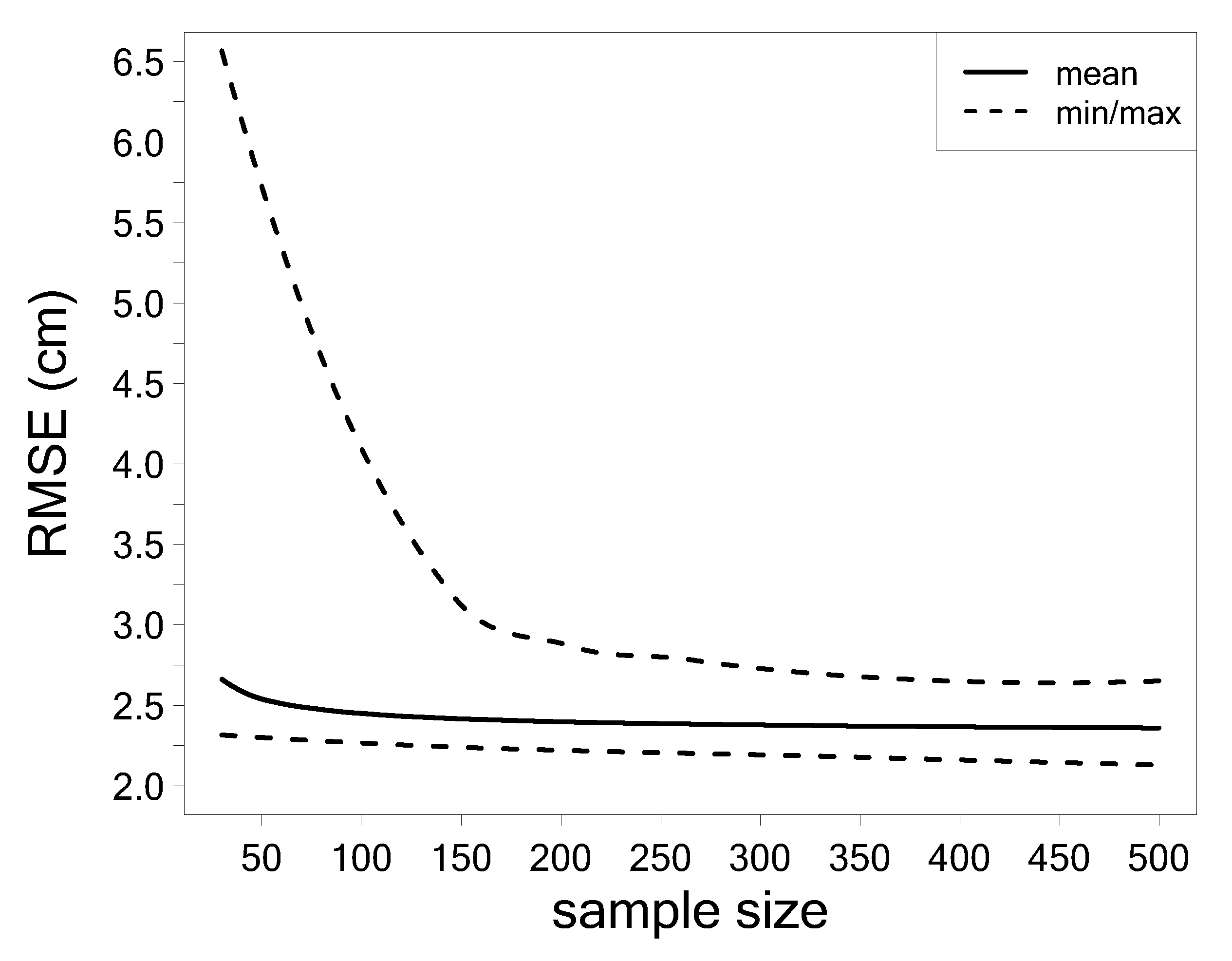
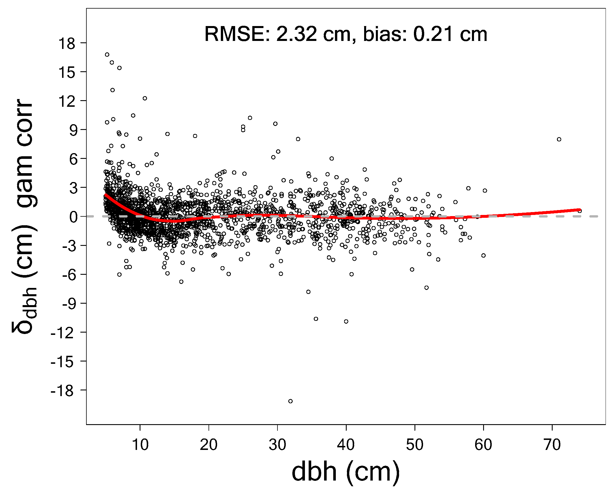
3.5. Diameter Correction

We found that dbh modeled with natural cubic splines had the lowest RMSE for PLS. Nevertheless, a bias depending on the reference diameter was also seen, as shown in Figure 8. The results of the cross-validation for the linear model to correct the estimated diameters can be found in Figure 11. It can be seen that the RMSE decreased with increasing number of measured reference diameters. The maximum RMSE could be kept below 2.70 cm and the average RMSE below 2.40 cm when using 250 or more manual reference measurements.

The model results for an example of 10,000 random samples used for modeling and validation can be found in

Table 4. Regression analysis.

		$\mathbf{dbh} \mathbf{Deviation} \mathit{\delta }$
Covariate	Coef.	Est.	SE	t Value	p Value
$\mathit{I}\mathit{n}\mathit{t}\mathit{e}\mathit{r}\mathit{c}\mathit{e}\mathit{p}\mathit{t}$	${\mathit{\beta }}_{\mathbf{0}}$	−9.770	3.355	−2.912	0.004
$\mathit{l}\mathit{o}\mathit{g}({\mathit{d}}_{\mathit{g}\mathit{a}\mathit{m}})$	${\mathit{\beta }}_{\mathbf{1}}$	−1.851	0.752	−6.727	<0.001
$\mathit{m}\mathit{e}\mathit{a}\mathit{n}\mathit{\_}\mathit{i}\mathit{n}\mathit{t}\mathit{e}\mathit{n}$	${\mathit{\beta }}_{\mathbf{2}}$	0.001	<0.001	3.371	<0.001
$\mathit{s}{\mathit{d}}_{\mathit{r}\mathit{e}\mathit{s}\mathit{\_}\mathit{g}\mathit{a}\mathit{m}}$	${\mathit{\beta }}_{\mathbf{3}}$	689.9	138.9	4.996	<0.001
$\mathit{m}\mathit{e}\mathit{a}\mathit{n}\mathit{\_}\mathit{i}\mathit{n}\mathit{t}\mathit{e}\mathit{n}\mathit{\times }\mathit{s}{\mathit{d}}_{\mathit{r}\mathit{e}\mathit{s}\mathit{\_}\mathit{g}\mathit{a}\mathit{m}}$	${\mathit{\beta }}_{\mathbf{4}}$	−0.045	0.010	−4.336	<0.001
${\mathit{R}}^{\mathbf{2}}$		0.353

SE, standard error; $R^2$, coefficient of determination.

. The dbh deviation $\left(\delta \right)$ decreased (in the sense of becoming more negative) as the estimated logarithmic dbh $\left(d_{gam}\right)$ increased. When the mean intensity ($mean\_inten$) and the standard deviation of residuals ($s{d}_{res\_gam}$ increased, the dbh deviation ($\delta$) also increased (in the sense of becoming more positive). The effect of mean intensity ($mean\_inten$) on dbh deviation decreased as the standard deviation of residuals ($s{d}_{res\_gam}$) increased. The coefficient of determination was 0.353 for the linear model.

An example of how the dbh deviations looked after correction by the linear model (using 250 reference diameters) is shown in Figure 12. The bias, for large diameters (dbh > 10 cm), widely disappeared; however, overestimation of small diameters (dbh < 10 cm) decreased only marginally and was still present. This resulted in a RMSE of 2.32 cm and a bias of 0.21 cm. A table with the performance, in terms of corrected dbh estimations separately for each sample plot, can be found in Appendix B, Table A4.

4. Discussion

4.1. Point Cloud Quality PLS/TLS

One of the major advantages of applying PLS (in this study: GeoSLAM ZEB HORIZON [64]) is rapid data acquisition over the entire forest plot. The PLS had some clear advantages over TLS when taking field measurements: it solved the TLS-related problems of setting up the system and using calibration targets on tripods. With a maximum number of 300,000 points per second and a maximum range of 100 m, the GeoSLAM ZEB HORIZON may also be well-suited to capturing tree heights and canopy shapes. However, this requires further research. The PLS combined with SLAM algorithms had better registration accuracies in forest environments, compared to MLS systems using GNSS data. The registration process for the points worked automatically and 100% of the PLS sample points were successfully registered. The process took approximately 30 min per sample plot on a notebook with 64 GB main memory and an i7-8750H hexa core CPU (Intel Corp., Santa Clara, CA, U.S.A.). Initial tests showed that the registration of the points with the SLAM algorithm worked without problems, up to a recording time of approximately 30 min. Real time data processing and visualization would be a convenient feature, as field crews could directly check if scanning worked properly. Scanners with lower range and data acquisition rate, like the GeoSLAM ZEB RevoRT already offer this feature, however, currently, the amount of data produced by the ZEB Horizon, is still too large to be processed in real time. Keeping Moore’s law in mind, it is however only a question of time until real time data visualization will be possible for scanners like the ZEB Horizon.

Longer recording times (up to 45 min) yielded instrumental drift and registration problems which resulted in the occurrence of doubled tree images. Moreover, the computing time and especially the amount of necessary main memory drastically increased: on a machine equipped with 64 GB of main memory, registration was impossible; on a machine equipped with 128 GB main memory and an i7-6850K hexa core CPU (Intel Corp., Santa Clara, CA, U.S.A.), registration took approximately 24h of computing time.

Due to the high cross-section completeness of the PLS scans, compared to TLS scans, there were also more flexible options for modeling the diameter, such as polygons [107] or free-form curves [108]. Nevertheless, the noise in the point clouds was higher for PLS than for TLS. Thus, problems occurred; especially with small diameters, as these no longer had a gap in the center. This could also lead to problems for modeling taper forms, as no reduction in the upper, smaller diameters was visible in the PLS point clouds. Applications such as modeling of branching architecture, bark structure, or tree species recognition could be limited due to this high PLS noise.

Future research questions in the area of PLS arise in dealing with the low precision of the 3D points. There will still be applications that can only be managed with TLS, due to their high precision requirements. However, PLS also opens up new possibilities for sample design. It is no longer necessary to make circular samples and, so, new methods could be developed; for example, using random walk approaches.

4.2. Stem Detection

The algorithm used in this study was developed and trained based on the sample plots of the BOKU forest inventory and worked fully automatically for PLS and TLS. Sample plots were intentionally selected to represent a broad range of stand and terrain conditions (stand density ranging from 286 trees ha⁻¹ to 3350 tress ha⁻¹, and slope ranging from 10.1% to 51.0 %), the results remain constant under all conditions. The TLS data acquisition was done one year before the PLS recordings, which means that, due to thinning and for a fair comparison, only 17 TLS sample plots were used. One advantage of our study was that the different scanning methods had the same pre-conditions regarding stem density, tree species, stem sizes, understory vegetation, reference data, and plot size. This made it easier to compare the PLS and TLS used in the study. Except for processing the raw scan data with the manufacturer’s software, point cloud processing and analysis was performed using R statistical software (R Foundation for Statistical Computing, Vienna, Austria) [83]. This was also an advantage, as the majority of the workload can be carried out with freely available and programmable software. For each sample plot and scanner system (PLS and TLS), constant parameter settings were applied for the underlying clustering algorithms and diameter fitting routines. There were only a few differences in the parameters of PLS and TLS algorithms (see Appendix A, Table A2), which were necessary mainly due to the higher point density in TLS. As a result, the proposed methodology proved to be robust and provided high flexibility under different forest structure scenarios and in different scanning setups.

The use of PLS resulted in a better tree detection rate than multi-scan TLS with a very competitive acquisition time. For PLS, the average detection rate and time required for a 20 m radius sample plot with a lower dbh threshold of 5 cm were 96% (sd ±4.84%) and 10.96 min (sd ±2.24 min), respectively. In comparison, the TLS detected 78.46% (sd ±16.22%) of trees in 49.6 min (sd ±0 min). The high number of non-detections with TLS can be explained by occlusion effects resulting from the small number of only four scan positions. The PLS provides a multi-view mapping scenario, which records each tree from different directions as the operator position and viewing geometry constantly changed and the entire plot was recorded by walking through it. The proportion of falsely detected trees (commission error) was 1.13% (sd ±2.12%) for PLS and 2.41% (sd ±2.76%) for TLS. Although the commission error for both was very low, TLS had about twice as many falsely detected trees as PLS. This was mainly due to TLS co-registration problems. It was shown that plot size and the lower dbh threshold in PLS had only a small influence, in contrast to that in TLS. The detection rate increased at 10 m radius and 10 cm lower dbh threshold to 99.49% (sd ±1.59%) for PLS and to 98.35% (sd ±4.01%) for TLS. This was because the density of the TLS 3D point cloud data became thinner and occlusion effects were more likely to occur with a higher distance from the scanner.

4.3. dbh Estimation

In dbh measurement, it was found that small diameters (dbh < 10 cm) were overestimated and large diameters (dbh > 10 cm) were underestimated with PLS, regardless of the fitting method. It turned out that the dbh modeled with natural cubic splines had the highest accuracy (RMSE: 2.87 cm) for PLS, with corresponding bias of −0.48 cm. An interpretation of the overall bias is meaningless, due to the dependency of the bias on the diameters. There were also differences between tree species, but the general trend that small diameters were overestimated and large diameters were underestimated remained the same. The reason for the overestimation of small trees was probably the high noise in the PLS point clouds: With increasing noise, in terms of $s{d}_{res\_gam}$, the overestimation increased.

In order to obtain exact diameter estimates from PLS, a correction model for $d_{gam}$ with the predictor variables $d_{gam}$, mean intensity of the points ($mean\_inten$), standard deviation of the residuals ($s{d}_{res\_gam}$), and interaction between the $mean\_inten$ and $s{d}_{res\_gam}$ was fitted. In the course of this, the diameter deviation should be predicted. The mean intensity was also a term for the tree dimension, which increased as the diameter increased. The point intensity also reflected the reflectivity of the surfaces and, thus, different tree species were represented to a certain extent. As the standard deviation of the residuals ($s{d}_{res\_gam}$) increased, the diameter error also increased. Cross-validation showed that at least 250 manual reference measurements are necessary to keep the RMSE below 2.40 cm. The large diameters showed, after correction, no underestimation; although, for small diameters, only a marginal reduction of the overestimation was seen. With regard to the correction, it could also be beneficial to measure the reference in diameter classes separately, according to tree species. This could reduce measurement costs and better consider differences in tree species. In order to control the underestimations of large trees, alternatively smooth additive regression models for quantiles were fitted with the function qgam() in the R package qgam [109], in order to see if there was an optimal quantile. However, the optimal quantile could only be predicted with a coefficient of determination of 0.28 using the preliminary estimated diameter $d_{gam}$ and, therefore, proved to be unsuitable.

The dbh estimates from TLS did not show a trend in diameter deviations, like for PLS estimates, and there were no tree species differences. The highest accuracy (RMSE: 2.55 cm) was achieved for TLS with an elliptical dbh fit. However, there were also high diameter deviations for TLS, which are explained mainly by co-registration problems. It seems that all diameter fitting methods tended to have outliers when the cross-sections of the stem were incomplete. Particularly in the outer areas of the sample plots, TLS had more incomplete cross-sections, compared to PLS. In this regard, it may be advantageous to place the outer scan positions of the TLS at the perimeter of the sample plot.

In principle, the performance of the algorithms used for the point cloud processing, position finding, and dbh measurement should not be influenced by seasonal effects. However, in the leaf-on stage during the vegetation period, the quality (completeness) of the point cloud is probably lower, due to shadowing effects. Particularly in deciduous forests, a high stem density and a multi-layered structure could more easily produce co-registration problems during the vegetation period. In order to provide clear results, further research is needed in the future on how the methods are affected by such seasonal effects.

4.4. Cylindrical Reference Objects

Using reference data collected on eight cylindrical objects, it was shown that the diameter was underestimated for all objects (i.e., regardless of their actual diameter). However, the noise, in terms of $s{d}_{res\_gam}$ in the reference data obtained under controlled conditions, was lower compared to the PLS scans in the forest. Concerning this, there was also a positive correlation with the scan time. The fact that the reference objects were underestimated even with small diameters (5 cm) was due to the small standard deviation of the residuals, compared to the data from the forest. Obviously, the systematic underestimation of PLS-derived diameters had device-related or software-related (SLAM) reasons.

4.5. Comparison with Other Studies

Table 5. Comparison of current results with previous studies.

Reference	Method	Scanner	TLS Scanner- Positions	Detection Rate (%)	Commis-sion Rate (%)	Overall Accuracy (%)	RMSE (cm)	Bias (cm)
This study	PLS	GeoSLAM ZEB HORIZON		96	1.1	94.9	2.32	0.21
	TLS	FARO Focus3D X330	4	78.5	2.4	76.1	2.55	−0.74
Bauwens et al. [49]	PLS	GeoSLAM ZEB1		90	31	59	1.11	−0.08
	TLS	FARO Focus 3D 120	5	93	22	71	1.30	−0.17
	TLS	FARO Focus 3D 120	1	78	21	57	3.73	−0.08
Oveland et al. [53]	PLS	GeoSLAM ZEB1		74.0	4.8	69.2	3.1	0.30
	TLS	FARO Focus3D X130	1	61.8	5.4	56.4	6.2	−2.00
Chen et al. [47]	PLS	GeoSLAM ZEB-REVO-RT		93.3	6.1	87.2	1.58	−1.26
Ryding et al. [46]	PLS	GeoSLAM ZEB1		*	*	*	2.90	−0.30

* Not evaluated against manual field data.

shows a comparison of the results of our study with other studies which evaluated SLAM-based PLS approaches. In particular, recent studies and those with TLS comparisons on the same sample plots were used. The GeoSLAM ZEB HORIZON used in our study represents the latest scanner generation from GeoSLAM. Compared to other studies, the highest detection rate and lowest commission rate were achieved with PLS. Regarding RMSE and bias, the results of the present study performed in the middle range. For further details on the comparative studies, the reader is referred to those. In Gollob et al. [20], where the same 17 TLS points were used as in this study, only 59.1% of the trees were found in a 20 m sample plot radius with a lower dbh threshold of 5 cm and using a different algorithm. It can be seen that there were also large differences due to the algorithms used, which makes it difficult to compare studies.

Bauwens et al. [49] also found a trend in the diameter deviations due to the tree size for the GeoSLAM ZEB1. In addition to the tree size, the bark roughness was also shown to have a significant effect on dbh estimates [49]. Furthermore, Brolly et al. [110] stated that the roughness of the bark seems to have influence in the accuracy of TLS dbh estimates. Ryding et al. [46] indicated that there was a significant difference in the fitting accuracy of trunks with diameters greater than 10 cm and less than 10 cm. In our study, tree species differences could also be found, but they did not change the general trend in diameter deviations due to tree size and were relatively small. The high noise in the PLS cross-sections may have masked the effect of bark roughness. Bauwens et al. [49] argued that the influence of the tree size for dbh estimates is based on the irregularity of the shape of cross-sections and the fact that smaller trees often have low branches and are surrounded by other small trees with low branches. We attempted to model such irregular shapes in our study with flexible curves ($d_{gam}$, $d_{tegam}$), but this did not result in much higher dbh precision and accuracy. The trends of overestimation (small diameters) and underestimation (large diameters) were still present. In this study, a test was also made to measure the diameter, similar to the method used in the field with calipers. Therefore, the non-circularly modeled cross-sections ($d_{gam}$, $d_{tegam}$, $d_{ell}$) were measured with rotating clipping boxes, in the same way as with a caliper from different directions. This also did not lead to more precise diameters.

Some studies [46,54] have indicated that PLS is 2 to 12 times faster in scanning time than TLS. However, this comparison must be viewed critically, with regard to different hardware parameter settings, number of TLS locations, and walking paths in PLS. Furthermore, the times for co-registration are usually not taken into account. In the present study, the scan time for PLS, with an average of 10.96 min per sample plot, was 4.6 times shorter than for TLS (49.9 min). In comparison, traditional inventory methods like the Bitterlich relascope sampling, which has been carried out on the same sample plots since 1989, took around 30 min per sample plot. The times mentioned were always recording times for one person doing the inventory. Further research is necessary for more informed statements regarding walking times to the sample plots, processing times for the 3D data and transfer times for the traditional inventories. In terms of a fair comparison, it is important to mention that the Bitterlich relascope sampling does not include the full tree pattern and no tree locations.

In this study, a star-shaped walking path was used, similar to Bauwens et al. [49], Oveland et al. [53], and Giannetti et al. [56]. The walking path influences the scanner range noise and drifts associated with the SLAM algorithm. Liang et al. [42] stated that, for PLS in general, it is important to plan the walking path before data acquisition. The results of the present study showed that the noise in the point clouds increased with the scan time. A recommendation for forest inventory on circular samples could be to make the radius smaller, in order to shorten the scanning time. However, a decreased sample plot size would require more sample plots to obtain the same level of inventory precision. As this would be associated with more working time for moving from plot to plot, studies on the optimal sample plot size for PLS are needed in the future. Ryding et al. [46] stated that, for the GeoSLAM ZEB1, a slower operational gait may also allow for a higher resolution point cloud creation. Del Perugia et al. [55] showed, in a study on the influence of scan density on the estimation of single-tree attributes by SLAM-based PLS, that a distance of 10 m between scan paths provided the best results with the GeoSLAM ZEB1. No such studies have yet been carried out for the new GeoSLAM ZEB HORIZON used in our study.

Due to the many possible combinations of parameter settings, such as hardware properties, scanner position variations, underlying forest structure diversity, and non-homogeneous quality criteria, comparative assessment of the results from different laser scanning studies is difficult [7]. For this reason, an international benchmark project [7] for TLS forest inventory has been initiated, in order to evaluate the performance of different algorithms under predefined reference conditions. To carry out an objective comparison of different routines for PLS forest inventory, a benchmark project for PLS or MLS would also be beneficial in the future. This is the reason why the PLS, TLS, and reference data from the sample plots of this study have been made freely available for research purposes.

4.6. Quality of Reference Data

The assessment of results from automatic laser scanning routines is usually based on manually collected field measurements. The tree position in the field measurement is defined as the cross-section center at a height of 1.3 m (i.e., breast height). If trees fork just above or below this height, it is not guaranteed that an automatic algorithm recognizes them and correctly detects the corresponding number of trees. The 1.3 m breast height should also be viewed critically. In forestry, the ground level (height = 0 m) is defined as the highest point of the ground around the tree; however, the algorithms used for tree detection and diameter estimation do not always use this definition. Frequently (as in this study), the point clouds are normalized with a DTM and, thus, the definition of breast height is violated. Another crucial step is the classification of terrain points. If the stem base is also classified as terrain, then the trees are made smaller due to normalization. In the current study, care was taken when choosing the parameters for terrain classification, such that terrain points were clearly separated from the stem bases. Errors in the 1.3 m breast height have an influence on the estimated positions and diameters and ensure, together with manual reference diameters measured at the wrong heights, imprecise results. A solution to this would be to mark the breast height before scanning and manual dbh measurements.

Irregularities at the base of the stem, such as ovality, might induce error in the measured diameter when using calipers, due to the measuring direction. During a manual field survey for this study, it was not always guaranteed that the specified measuring direction was followed. In order to take this into account, trials were made to test different measuring directions with clipping boxes rotating around the modeled cross-sections. This did not lead to more precise diameter estimates. However, the high noise in the PLS data may have masked the influence of the measuring direction. For the incomplete TLS cross-sections, an evaluation of the measuring direction was not meaningful. On the other hand, least-square fitting methods on irregular cross-sections, as well as on trees with rough bark, induce lower diameter estimates than with caliper measurement. Tilted trees are another problem: according to the field measurement instructions, tilted trees were also measured at an angle using the calipers. Many automatic laser scanning routines (including that in this study) do not take the tilt of the trees into account.

Luoma et al. [111] assessed the precision in conventional field measurements of individual tree attributes. A total of 319 sample trees were measured independently by four trained mensurationists. The standard deviations in tree dbh and height measurements were 0.3 cm (1.5%) and 0.5 m (2.9%), respectively. There were no statistically significant differences for tree species and tree size classes between the obtained dbh or height measurements. These results are important when using sample plot data in forest inventory applications; especially now, at a time when new tree attribute measurement techniques based on remote sensing are being developed and compared to conventional caliper and clinometer measurements.

5. Conclusions

The major goal of the present study was to investigate the accuracy of tree detection and diameter estimation in forest inventory using PLS under various stand and terrain conditions. A new SLAM-based personal laser scanner (PLS) was used for this and, to the best of our knowledge, this represents the first application of this scanner in a forestry context. The results of the PLS data were compared with TLS results on the same inventory plots, using a new algorithm for automatic tree detection and dbh estimation. Our tree detection and diameter estimation method proved to be applicable to manifold forest structure conditions comprising different species combinations, varying stem densities, and dense understory vegetation. Parameter setup of the scanning devices was kept fixed for PLS and TLS scans under all environmental conditions, so that the field crews did not have to change the setup. Additionally, the parameter setup of the algorithms for extracting tree attributes from the point cloud were unchanged, so that these extractions worked fully automated. It was shown that, with PLS, 96% of trees could be detected in a 20 m sample plot radius with a lower dbh threshold of 5 cm. The proportion of falsely detected trees was 1.1%. In comparison, TLS detected 78.5% of the trees with a percentage of falsely detected trees of 2.4%. Using plot radii of 20 m, 15 m, and 10 m, as well as a lower dbh threshold of 10 cm, the respective detection rates for PLS were 98.76%, 98.95%, and 99.48%, while the respective detection rates for TLS were considerably lower (86.32%, 93.81%, and 98.35%), especially for larger sample plots. Different methods for diameter estimation were tested for PLS and TLS. Regarding diameter estimation, there was a trend in the diameter deviations of PLS which depended on the tree size. However, this trend was corrected with a function, resulting in a RMSE of 2.32 cm (12.01%) and a bias of 0.21 cm (1.09%) for the best diameter estimation method ($d_{gam}$). With TLS, an accuracy, in terms of RMSE, of 2.55 cm (13.19%) and a precision, in terms of bias, of −0.74 cm (−3.83%) was achieved with the best diameter estimation method ($d_{ell}$). The scan time for PLS, with an average of 10.96 min per sample plot, was 4.6 times shorter than for TLS (49.9 min).

Decision-making in forest resources relies on precise information collected using sample-based inventories. With traditional instruments, such as calipers and tapes, the entire workflow—from data collection to data analysis—can be regarded as inefficient. In contrast, information is kept electronically throughout the entire workflow of laser-based surveys. Thus, high-resolution 3D data remains accessible with novel software routines in the future. PLS technology represents the next step (i.e., after TLS technology) towards an efficient and modern forest inventory methodology. It is also expected that PLS will be more often used in forest inventories as soon as the currently developed programs are available, in terms of free software routines, and the challenges of imprecise PLS point clouds are solved.

References

1. Wendland, A.; Bawa, K.S. Tropical forestry: The costa rican experience in management of forest resources. J. Sustain. For. 1996, 3, 91–156. [Google Scholar] [CrossRef]
2. Kershaw, J.A.; Ducey, M.J.; Beers, T.W.; Husch, B. Forest Mensuration; John Wiley & Sons, Ltd.: Chichester, UK, 2016; ISBN 9781118902028. [Google Scholar]
3. Köhl, M.; Magnussen, S.; Marchetti, M. Sampling Methods, Remote Sensing and GIS Multiresource Forest Inventory; Tropical Forestry; Springer Berlin Heidelberg: Berlin, Heidelberg, 2006; ISBN 978-3-540-32571-0. [Google Scholar]
4. Kauffman, J.B.; Arifanti, V.B.; Basuki, I.; Kurnianto, S.; Novita, N.; Murdiyarso, D.; Donato, D.C.; Warren, M.W. Protocols for the Measurement, Monitoring, and Reporting of Structure, Biomass, Carbon Stocks and Greenhouse Gas Emissions in Tropical Peat Swamp Forests; Center for International Forestry Research (CIFOR): Bogor, Indonesia, 2017. [Google Scholar]
5. Kramer, H.; Akça, A. Leitfaden zur Waldmesslehre; J. D. Sauerländers Verlag: Bad Orb, Germany, 2008. [Google Scholar]
6. Liang, X.; Kankare, V.; Hyyppä, J.; Wang, Y.; Kukko, A.; Haggrén, H.; Yu, X.; Kaartinen, H.; Jaakkola, A.; Guan, F.; et al. Terrestrial laser scanning in forest inventories. ISPRS J. Photogramm. Remote Sens. 2016, 115, 63–77. [Google Scholar] [CrossRef]
7. Liang, X.; Hyyppä, J.; Kaartinen, H.; Lehtomäki, M.; Pyörälä, J.; Pfeifer, N.; Holopainen, M.; Brolly, G.; Francesco, P.; Hackenberg, J.; et al. International benchmarking of terrestrial laser scanning approaches for forest inventories. ISPRS J. Photogramm. Remote Sens. 2018, 144, 137–179. [Google Scholar] [CrossRef]
8. Ritter, T.; Schwarz, M.; Tockner, A.; Leisch, F.; Nothdurft, A. Automatic mapping of forest stands based on three-dimensional point clouds derived from terrestrial laser-scanning. Forests 2017, 8, 265. [Google Scholar] [CrossRef]
9. Liang, X.; Kukko, A.; Hyyppä, J.; Lehtomäki, M.; Pyörälä, J.; Yu, X.; Kaartinen, H.; Jaakkola, A.; Wang, Y. In-situ measurements from mobile platforms: An emerging approach to address the old challenges associated with forest inventories. ISPRS J. Photogramm. Remote Sens. 2018, 143, 97–107. [Google Scholar] [CrossRef]
10. Watt, P.J.; Donoghue, D.N.M. Measuring forest structure with terrestrial laser scanning. Int. J. Remote Sens. 2005, 26, 1437–1446. [Google Scholar] [CrossRef]
11. Maas, H.-G.; Bienert, A.; Scheller, S.; Keane, E. Automatic forest inventory parameter determination from terrestrial laser scanner data. Int. J. Remote Sens. 2008, 29, 1579–1593. [Google Scholar] [CrossRef]
12. Vonderach, C.; Vögtle, T.; Adler, P.; Norra, S. Terrestrial laser scanning for estimating urban tree volume and carbon content. Int. J. Remote Sens. 2012, 33, 6652–6667. [Google Scholar] [CrossRef]
13. Liu, J.; Liang, X.; Hyyppä, J.; Yu, X.; Lehtomäki, M.; Pyörälä, J.; Zhu, L.; Wang, Y.; Chen, R. Automated matching of multiple terrestrial laser scans for stem mapping without the use of artificial references. Int. J. Appl. Earth Obs. Geoinf. 2017, 56, 13–23. [Google Scholar] [CrossRef] [Green Version]
14. Ritter, T.; Nothdurft, A. Automatic assessment of crown projection area on single trees and stand-level, based on three-dimensional point clouds derived from terrestrial laser-scanning. Forests 2018, 9, 237. [Google Scholar] [CrossRef] [Green Version]
15. Henning, J.G.; Radtke, P.J. Detailed Stem Measurements of Standing Trees from Ground-Based Scanning Lidar. For. Sci. 2006, 52, 67–80. [Google Scholar] [CrossRef]
16. Moorthy, I.; Miller, J.R.; Berni, J.A.J.; Zarco-Tejada, P.; Hu, B.; Chen, J. Field characterization of olive (Olea europaea L.) tree crown architecture using terrestrial laser scanning data. Agric. For. Meteorol. 2011, 151, 204–214. [Google Scholar] [CrossRef]
17. Strahler, A.H.; Jupp, D.L.; Woodcock, C.E.; Schaaf, C.B.; Yao, T.; Zhao, F.; Yang, X.; Lovell, J.; Culvenor, D.; Newnham, G.; et al. Retrieval of forest structural parameters using a ground-based lidar instrument (Echidna ®). Can. J. Remote Sens. 2008, 34, S426–S440. [Google Scholar] [CrossRef] [Green Version]
18. Moskal, L.M.; Zheng, G. Retrieving forest inventory variables with terrestrial laser scanning (TLS) in urban heterogeneous forest. Remote Sens. 2012, 4, 1–20. [Google Scholar] [CrossRef] [Green Version]
19. Schilling, A.; Schmidt, A.; Maas, H.-G. Tree Topology Representation from TLS Point Clouds Using Depth-First Search in Voxel Space. Photogramm. Eng. Remote Sens. 2012, 78, 383–392. [Google Scholar] [CrossRef]
20. Gollob, C.; Ritter, T.; Wassermann, C.; Nothdurft, A. Influence of Scanner Position and Plot Size on the Accuracy of Tree Detection and Diameter Estimation Using Terrestrial Laser Scanning on Forest Inventory Plots. Remote Sens. 2019, 11, 1602. [Google Scholar] [CrossRef] [Green Version]
21. Piermattei, L.; Karel, W.; Wang, D.; Wieser, M.; Mokroš, M.; Surový, P.; Koreň, M.; Tomaštík, J.; Pfeifer, N.; Hollaus, M. Terrestrial Structure from Motion Photogrammetry for Deriving Forest Inventory Data. Remote Sens. 2019, 11, 950. [Google Scholar] [CrossRef] [Green Version]
22. Panagiotidis, D.; Surový, P.; Kuželka, K. Accuracy of Structure from Motion models in comparison with terrestrial laser scanner for the analysis of DBH and height influence on error behaviour. J. For. Sci. 2016, 62, 357–365. [Google Scholar] [CrossRef] [Green Version]
23. Mikita, T.; Janata, P.; Surový, P.; Hyyppä, J.; Liang, X.; Puttonen, E. Forest Stand Inventory Based on Combined Aerial and Terrestrial Close-Range Photogrammetry. Forests 2016. [Google Scholar] [CrossRef] [Green Version]
24. Mokroš, M.; Liang, X.; Surový, P.; Valent, P.; Nava, J.; Chudý, F.; Tunák, D.; SaloňSaloˇSaloň, Š.; Merganič, J. Geo-Information Evaluation of Close-Range Photogrammetry Image Collection Methods for Estimating Tree Diameters. ISPRS Int. J. Geo-Inf. 2018. [Google Scholar] [CrossRef] [Green Version]
25. Liu, J.; Feng, Z.; Yang, L.; Mannan, A.; Khan, T.U.; Zhao, Z.; Cheng, Z. Extraction of sample plot parameters from 3D point cloud reconstruction based on combined RTK and CCD continuous photography. Remote Sens. 2018, 10. [Google Scholar] [CrossRef] [Green Version]
26. Liang, X.; Jaakkola, A.; Wang, Y.; Hyyppä, J.; Honkavaara, E.; Liu, J.; Kaartinen, H. Remote sensing The Use of a Hand-Held Camera for Individual Tree 3D Mapping in Forest Sample Plots. Remote Sens. 2014, 6, 6587–6603. [Google Scholar] [CrossRef] [Green Version]
27. Liang, X.; Wang, Y.; Jaakkola, A.; Kukko, A.; Kaartinen, H.; Hyyppa, J.; Honkavaara, E.; Liu, J. Forest Data Collection Using Terrestrial Image-Based Point Clouds From a Handheld Camera Compared to Terrestrial and Personal Laser Scanning. IEEE Trans. Geosci. Remote Sens. 2015, 53, 5117–5132. [Google Scholar] [CrossRef]
28. Maltamo, M.; Næsset, E.; Manag, J.V.-C. Concepts and Case Studies. In Forestry Applications of Airborne Laser Scanning; Springer: Berlin, Germany, 2014. [Google Scholar]
29. Lindberg, E.; Hollaus, M. Comparison of methods for estimation of stem volume, stem number and basal area from airborne laser scanning data in a hemi-boreal forest. Remote Sens. 2012, 4, 1004–1023. [Google Scholar] [CrossRef] [Green Version]
30. Korhonen, L.; Vauhkonen, J.; Virolainen, A.; Hovi, A.; Korpela, I. Estimation of tree crown volume from airborne lidar data using computational geometry. Int. J. Remote Sens. 2013, 34, 7236–7248. [Google Scholar] [CrossRef]
31. Vauhkonen, J.; Næsset, E.; Gobakken, T. Deriving airborne laser scanning based computational canopy volume for forest biomass and allometry studies. ISPRS J. Photogramm. Remote Sens. 2014, 96, 57–66. [Google Scholar] [CrossRef]
32. Yu, X.; Hyyppä, J.; Kaartinen, H.; Maltamo, M. Automatic detection of harvested trees and determination of forest growth using airborne laser scanning. Remote Sens. Environ. 2004, 90, 451–462. [Google Scholar] [CrossRef]
33. Brede, B.; Calders, K.; Lau, A.; Raumonen, P.; Bartholomeus, H.M.; Herold, M.; Kooistra, L. Non-destructive tree volume estimation through quantitative structure modelling: Comparing UAV laser scanning with terrestrial LIDAR. Remote Sens. Environ. 2019, 233. [Google Scholar] [CrossRef]
34. Puliti, S.; Dash, J.P.; Watt, M.S.; Breidenbach, J.; Pearse, G.D. A comparison of UAV laser scanning, photogrammetry and airborne laser scanning for precision inventory of small-forest properties. For. An Int. J. For. Res. 2019. [Google Scholar] [CrossRef]
35. Brede, B.; Lau, A.; Bartholomeus, H.; Kooistra, L. Comparing RIEGL RiCOPTER UAV LiDAR Derived Canopy Height and DBH with Terrestrial LiDAR. Sensors 2017, 17, 2371. [Google Scholar] [CrossRef]
36. Li, J.; Yang, B.; Cong, Y.; Cao, L.; Fu, X.; Dong, Z. 3D forest mapping using a low-cost UAV laser scanning system: Investigation and comparison. Remote Sens. 2019, 11. [Google Scholar] [CrossRef] [Green Version]
37. Bruggisser, M.; Hollaus, M.; Kükenbrink, D.; Pfeifer, N. Comparison of Forest Structure Metrics Derived from Uav Lidar and Als Data. In Proceedings of the ISPRS Annals of the Photogrammetry, Remote Sensing and Spatial Information Sciences; Copernicus GmbH, Bergamo, Italy, 6–8 February 2019; Volume 4, pp. 325–332. [Google Scholar]
38. Cao, L.; Liu, H.; Fu, X.; Zhang, Z.; Shen, X.; Ruan, H. Comparison of UAV LiDAR and Digital Aerial Photogrammetry Point Clouds for Estimating Forest Structural Attributes in Subtropical Planted Forests. Forests 2019, 10, 145. [Google Scholar] [CrossRef] [Green Version]
39. Puliti, S.; Solberg, S.; Granhus, A. Use of UAV Photogrammetric Data for Estimation of Biophysical Properties in Forest Stands Under Regeneration. Remote Sens. 2019, 11, 233. [Google Scholar] [CrossRef] [Green Version]
40. Krause, S.; Sanders, T.G.M.; Mund, J.-P.; Greve, K. UAV-Based Photogrammetric Tree Height Measurement for Intensive Forest Monitoring. Remote Sens. 2019, 11, 758. [Google Scholar] [CrossRef] [Green Version]
41. Surový, P.; Almeida Ribeiro, N.; Panagiotidis, D. Estimation of positions and heights from UAV-sensed imagery in tree plantations in agrosilvopastoral systems. Int. J. Remote Sens. 2018, 39, 4786–4800. [Google Scholar] [CrossRef]
42. Liang, X.; Kukko, A.; Kaartinen, H.; Hyyppä, J.; Yu, X.; Jaakkola, A.; Wang, Y. Possibilities of a Personal Laser Scanning System for Forest Mapping and Ecosystem Services. Sensors 2014, 14, 1228–1248. [Google Scholar] [CrossRef]
43. Maltamo, M.; Bollandsas, O.M.; Naesset, E.; Gobakken, T.; Packalen, P. Different plot selection strategies for field training data in ALS-assisted forest inventory. Forestry 2011, 84, 23–31. [Google Scholar] [CrossRef] [Green Version]
44. Holopainen, M.; Kankare, V.; Vastaranta, M.; Liang, X.; Lin, Y.; Vaaja, M.; Yu, X.; Hyyppä, J.; Hyyppä, H.; Kaartinen, H.; et al. Tree mapping using airborne, terrestrial and mobile laser scanning—A case study in a heterogeneous urban forest. Urban For. Urban Green. 2013, 12, 546–553. [Google Scholar] [CrossRef]
45. Liang, X.; Hyyppa, J.; Kukko, A.; Kaartinen, H.; Jaakkola, A.; Yu, X. The Use of a Mobile Laser Scanning System for Mapping Large Forest Plots. IEEE Geosci. Remote Sens. Lett. 2014, 11, 1504–1508. [Google Scholar] [CrossRef]
46. Ryding, J.; Williams, E.; Smith, M.; Eichhorn, M. Assessing Handheld Mobile Laser Scanners for Forest Surveys. Remote Sens. 2015, 7, 1095–1111. [Google Scholar] [CrossRef] [Green Version]
47. Chen, S.; Liu, H.; Feng, Z.; Shen, C.; Chen, P. Applicability of personal laser scanning in forestry inventory. PLoS ONE 2019, 14, e0211392. [Google Scholar] [CrossRef] [PubMed]
48. Pueschel, P.; Newnham, G.; Rock, G.; Udelhoven, T.; Werner, W.; Hill, J. The influence of scan mode and circle fitting on tree stem detection, stem diameter and volume extraction from terrestrial laser scans. ISPRS J. Photogramm. Remote Sens. 2013, 77, 44–56. [Google Scholar] [CrossRef]
49. Bauwens, S.; Bartholomeus, H.; Calders, K.; Lejeune, P. Forest Inventory with Terrestrial LiDAR: A Comparison of Static and Hand-Held Mobile Laser Scanning. Forests 2016, 7, 127. [Google Scholar] [CrossRef] [Green Version]
50. Bienert, A.; Georgi, L.; Kunz, M.; Maas, H.G.; von Oheimb, G. Comparison and combination of mobile and terrestrial laser scanning for natural forest inventories. Forests 2018, 8, 395. [Google Scholar] [CrossRef] [Green Version]
51. Rönnholm, P.; Liang, X.; Kukko, A.; Jaakkola, A.; Hyyppä, J. Quality Analysis and correction of mobile backpack laser scanning data. ISPRS Ann. Photogramm. Remote Sens. Spat. Inf. Sci. 2016, III–1, 41–47. [Google Scholar] [CrossRef]
52. Tjernqvist, M. Backpack-based Inertial Navigation and LiDAR Mapping in Forest Environments; Umeå University: Umeå, Sweden, 2017. [Google Scholar]
53. Oveland, I.; Hauglin, M.; Giannetti, F.; Kjørsvik, N.S.; Gobakken, T. Comparing three different ground based laser scanning methods for tree stem detection. Remote Sens. 2018, 10, 538. [Google Scholar] [CrossRef] [Green Version]
54. Cabo, C.; Del Pozo, S.; Rodríguez-Gonzálvez, P.; Ordóñez, C.; González-Aguilera, D. Comparing terrestrial laser scanning (TLS) and wearable laser scanning (WLS) for individual tree modeling at plot level. Remote Sens. 2018, 10, 540. [Google Scholar] [CrossRef] [Green Version]
55. Del Perugia, B.; Giannetti, F.; Chirici, G.; Travaglini, D. Influence of Scan Density on the Estimation of Single-Tree Attributes by Hand-Held Mobile Laser Scanning. Forests 2019, 10, 277. [Google Scholar] [CrossRef] [Green Version]
56. Giannetti, F.; Puletti, N.; Quatrini, V.; Travaglini, D.; Bottalico, F.; Corona, P.; Chirici, G. Integrating terrestrial and airborne laser scanning for the assessment of single-tree attributes in Mediterranean forest stands. Eur. J. Remote Sens. 2018, 51, 795–807. [Google Scholar] [CrossRef] [Green Version]
57. Vatandaşlar, C.; Zeybek, M. Application of handheld laser scanning technology for forest inventory purposes in the NE Turkey. Turkish J. Agric. For. 2020. [Google Scholar] [CrossRef]
58. Zhou, S.; Kang, F.; Li, W.; Kan, J.; Zheng, Y.; He, G. Extracting Diameter at Breast Height with a Handheld Mobile LiDAR System in an Outdoor Environment. Sensors 2019, 19, 3212. [Google Scholar] [CrossRef] [PubMed] [Green Version]
59. Kukko, A.; Kaijaluoto, R.; Kaartinen, H.; Lehtola, V.V.; Jaakkola, A.; Hyyppä, J. Graph SLAM correction for single scanner MLS forest data under boreal forest canopy. ISPRS J. Photogramm. Remote Sens. 2017, 132, 199–209. [Google Scholar] [CrossRef]
60. Thrun, S.; Montemerlo, M. The Graph SLAM Algorithm with Applications to Large-Scale Mapping of Urban Structures. Int. J. Robot. Res. 2006. [Google Scholar] [CrossRef]
61. ZEB Revo—GeoSLAM. Available online: https://geoslam.com/solutions/zeb-revo/ (accessed on 12 January 2020).
62. ZEB Revo RT—GeoSLAM. Available online: https://geoslam.com/solutions/zeb-revo-rt/ (accessed on 12 January 2020).
63. Abegg, M.; Kükenbrink, D.; Zell, J.; Schaepman, M.; Morsdorf, F.; Abegg, M.; Kükenbrink, D.; Zell, J.; Schaepman, M.E.; Morsdorf, F. Terrestrial Laser Scanning for Forest Inventories—Tree Diameter Distribution and Scanner Location Impact on Occlusion. Forests 2017, 8, 184. [Google Scholar] [CrossRef] [Green Version]
64. ZEB Horizon—GeoSLAM. Available online: https://geoslam.com/solutions/zeb-horizon/ (accessed on 13 January 2020).
65. Schodterer, H. Einrichtung eines Permanenten Stichprobennetzes im Lehrforst; University of Natural Resources and Life Sciences: Wien, Austria, 1987. [Google Scholar]
66. Bitterlich, W. Die Winkelzählprobe. Allgemeine forst-und holzwirtschaftliche Zeitung 1948, 59, 4–5. [Google Scholar] [CrossRef]
67. Bitterlich, W. Die Winkelzählprobe. Forstwiss. Cent. 1952, 71, 215–225. [Google Scholar] [CrossRef]
68. Bitterlich, W. The Relascope Idea. Relative Measurements in Forestry; Commonwealth Agricultural Bureau: Oxfordshire, UK, 1984; ISBN 0851985394. [Google Scholar]
69. Reineke, L.H. Perfecting a stand-density index for evenage forests. J. Agric. Res. 1933, 46, 627–638. [Google Scholar]
70. Fueldner, K. Strukturbeschreibung von Buchen-Edellaubholz-Mischwäldern; Georg-August-Universitaet Goettingen: Göttingen, Germany, 1995. [Google Scholar]
71. Clark, P.J.; Evans, F.C. Distance to Nearest Neighbor as a Measure of Spatial Relationships in Populations. Ecology 1954, 35, 445–453. [Google Scholar] [CrossRef]
72. Shannon, C.E. A Mathematical Theory of Communication. Bell Syst. Tech. J. 1948, 27, 379–423. [Google Scholar] [CrossRef] [Green Version]
73. PuckTM|Velodyne Lidar. Available online: https://velodynelidar.com/products/puck/ (accessed on 13 January 2020).
74. Hub—GeoSLAM. Available online: https://geoslam.com/solutions/geoslam-hub/ (accessed on 13 January 2020).
75. LAS (LASer) File Format, Version 1. Available online: https://www.loc.gov/preservation/digital/formats/fdd/fdd000418.shtml (accessed on 20 February 2020).
76. FARO SCENE|FARO Technologies. Available online: https://www.faro.com/products/construction-bim-cim/faro-scene/ (accessed on 23 February 2019).
77. Tan, K.; Zhang, W.; Shen, F.; Cheng, X. Investigation of TLS Intensity Data and Distance Measurement Errors from Target Specular Reflections. Remote Sens. 2018, 10, 1077. [Google Scholar] [CrossRef] [Green Version]
78. Kashani, A.; Olsen, M.; Parrish, C.; Wilson, N. A Review of LIDAR Radiometric Processing: From Ad Hoc Intensity Correction to Rigorous Radiometric Calibration. Sensors 2015, 15, 28099–28128. [Google Scholar] [CrossRef] [PubMed] [Green Version]
79. Tan, K.; Cheng, X. Correction of Incidence Angle and Distance Effects on TLS Intensity Data Based on Reference Targets. Remote Sens. 2016, 8, 251. [Google Scholar] [CrossRef] [Green Version]
80. Yan, W.Y.; Shaker, A.; El-Ashmawy, N. Urban land cover classification using airborne LiDAR data: A review. Remote Sens. Environ. 2015, 158, 295–310. [Google Scholar] [CrossRef]
81. Pfeifer, N.; Briese, C. Laser scanning—Principles and applications. In Proceedings of the GeoSiberia 2007—International Exhibition and Scientific Congress, Novosibirsk, Russia, 25 April 2007; EAGE Publications BV: Houten, The Netherlands, 2014. [Google Scholar]
82. FARO Laser Scanner Focus3D X 330 Features, Benefits & Technical Specifications. Available online: https://faro.app.box.com/s/8ilpeyxcuitnczqgsrgp5rx4a9lb3skq/file/441668110322 (accessed on 29 April 2020).
83. R Core Team. R: A Language and Environment for Statistical Computing; R Version 3.5.1; R Foundation for Statistical Computing: Vienna, Austria, 2018. [Google Scholar]
84. Dowle, M.; Srinivasan, A.; Gorecki, J.; Chirico, M.; Stetsenko, P.; Short, T.; Lianoglou, S.; Antonyan, E.; Bonsch, M.; Parsonage, H.; et al. Data.Table: Extension of “Data.Frame”, version 1.12.8. CRAN 2019.
85. Roussel, J.-R.; De Boissieu, F. rlas: Read and Write “las” and “laz” Binary File Formats Used for Remote Sensing Data 2019; R Foundation for Statistical Computing: Vienna, Austria, 2019. [Google Scholar]
86. Roussel, J.-R.; Auty, D.; Romain, J.-R.; Auty, D.; De Boissieu, F.; Meador Sánchez, A. lidR: Airborne LiDAR Data Manipulation and Visualization for Forestry Applications 2019; R Foundation for Statistical Computing: Vienna, Austria, 2019. [Google Scholar]
87. Zhang, W.; Qi, J.; Wan, P.; Wang, H.; Xie, D.; Wang, X.; Yan, G. An Easy-to-Use Airborne LiDAR Data Filtering Method Based on Cloth Simulation. Remote Sens. 2016, 8, 501. [Google Scholar] [CrossRef]
88. Ankerst, M.; Breunig, M.M.; Kriegel, H.P.; Sander, J. OPTICS: Ordering Points to Identify the Clustering Structure. ACM Sigmod Record 1999, 28, 49–60. [Google Scholar] [CrossRef]
89. Ester, M.; Kriegel, H.-P.; Sander, J.; Xu, X. A Density-Based Algorithm for Discovering Clusters in Large Spatial Databases with Noise. In Proceedings of the KDD’96: Second International Conference on Knowledge Discovery and Data Mining, Portland, OR, USA, 2–4 August 1996. [Google Scholar]
90. Ferrara, R.; Virdis, S.G.P.; Ventura, A.; Ghisu, T.; Duce, P.; Pellizzaro, G. An automated approach for wood-leaf separation from terrestrial LIDAR point clouds using the density based clustering algorithm DBSCAN. Agric. For. Meteorol. 2018, 262, 434–444. [Google Scholar] [CrossRef]
91. Birant, D.; Kut, A. ST-DBSCAN: An algorithm for clustering spatial–temporal data. Data Knowl. Eng. 2007, 60, 208–221. [Google Scholar] [CrossRef]
92. Eisenkeil, F.; Schafhitzel, T.; Kühne, U.; Deussen, O. Clustering and visualization of non-classified points from LiDAR Data for Helicopter Navigation. In Proceedings of the Signal Processing, Sensor/Information Fusion, and Target Recognition XXIII. International Society for Optics and Photonics, Baltimore, MD, USA, 5–8 May 2014; p. 90910V. [Google Scholar]
93. De Conto, T. TreeLS: Terrestrial Point Cloud Processing of Forest Data 2019; The Comprehensive R Archive Network: Wien, Austria, 2019. [Google Scholar]
94. Müller, C.H.; Garlipp, T. Simple consistent cluster methods based on redescending M-estimators with an application to edge identification in images. J. Multivar. Anal. 2005, 92, 359–385. [Google Scholar] [CrossRef] [Green Version]
95. Garlipp, T. edci: Edge Detection and Clustering in Images, R package version 1.1-3. 2018. Available online: https://CRAN.R-project.org/package=edci (accessed on 23 February 2019).
96. Fitzgibbon, A.W.; Pilu, M.; Fisher, R.B. Direct least squares fitting of ellipses. In Proceedings of the International Conference on Pattern Recognition, Vienna, Austria, 25–29 August 1996; Institute of Electrical and Electronics Engineers Inc.: New York, NY, USA, 1996; Volume 1, pp. 253–257. [Google Scholar]
97. Gama, J.; Chernov, N. conicfit: Algorithms for Fitting Circles, Ellipses and Conics Based on the Work by Prof. Nikolai Chernov 2015; R Foundation for Statistical Computing: Vienna, Austria, 2015. [Google Scholar]
98. Chernov, N. Circular and Linear Regression; CRC Press: Boca Raton, FL, USA, 2010. [Google Scholar]
99. Wood, S.N. Fast stable restricted maximum likelihood and marginal likelihood estimation of semiparametric generalized linear models. J. R. Stat. Soc. 2011, 73, 3–36. [Google Scholar] [CrossRef] [Green Version]
100. Wood, S.N.; Pya, N.; Säfken, B. Smoothing parameter and model selection for general smooth models (with discussion). J. Am. Stat. Assoc. 2016, 111, 1548–1575. [Google Scholar] [CrossRef]
101. Wood, S.N. Stable and efficient multiple smoothing parameter estimation for generalized additive models. J. Am. Stat. Assoc. 2004, 99, 673–686. [Google Scholar] [CrossRef] [Green Version]
102. Wood, S.N. Generalized Additive Models: An Introduction with R, 2nd ed.; Chapman and Hall/CRC: Boca Raton, FL, USA, 2017. [Google Scholar]
103. Wood, S.N. Thin-plate regression splines. J. R. Stat. Soc. 2003, 65, 95–114. [Google Scholar] [CrossRef]
104. Baddeley, A.; Turner, R. {spatstat}: An {R} Package for Analyzing Spatial Point Patterns. J. Stat. Softw. 2005, 12, 1–42. [Google Scholar] [CrossRef] [Green Version]
105. Girardeau-Montaut, D.C. 3D Point Cloud and Mesh Processing Software; Telecom ParisTechs: Palaiseau, France, 2017. [Google Scholar]
106. CRAN—Package vec2dtransf. Available online: https://cran.r-project.org/web/packages/vec2dtransf/index.html (accessed on 8 May 2020).
107. Wezyk, P.; Koziol, K.; Glista, M.; Pierzchalski, M. Terrestrial laser scanning versus traditional forest inventory first results from the polish forests. In Proceedings of the ISPRS Workshop on Laser Scanning 2007 and SilviLaser 2007, Espoo, Finland, 12–14 September 2007; Volume 36, pp. 424–429. [Google Scholar]
108. Pfeifer, N.; Winterhalder, D. Modelling of tree cross sections from terrestrial laser scanning data with free-form curves. Int. Arch. Photogramm. Remote Sens. Spat. Inf. Sci. 2004, 36, 76–81. [Google Scholar]
109. Fasiolo, M.; Wood, S.N.; Zaffran, M.; Nedellec, R.; Goude, Y. Fast Calibrated Additive Quantile Regression. J. Am. Stat. Assoc. 2020. [Google Scholar] [CrossRef] [Green Version]
110. Brolly, G.; Király, G. Algorithms for Stem Mapping by Means of Terrestrial Laser Scanning. Acta Silv. Lignaria Hung. 2009, 5, 119–130. [Google Scholar]
111. Luoma, V.; Saarinen, N.; Wulder, M.; White, J.; Vastaranta, M.; Holopainen, M.; Hyyppä, J. Assessing Precision in Conventional Field Measurements of Individual Tree Attributes. Forests 2017, 8, 38. [Google Scholar] [CrossRef] [Green Version]
112. Gollob, C.; Ritter, T.; Nothdurft, A. LAUT—Terrestrial and Personal laser scanner data from Austrian forest Inventory plots. Zenodo 2020. [Google Scholar] [CrossRef]
Figure 1. (a) ZEB HORIZON personal laser scanning (PLS) in operation; and (b) walking path for PLS data acquisition (starting and ending in plot center) and sample plot.
Remotesensing 12 01509 g001
Figure 2. (a) Cross-section of a single tree for PLS and terrestrial laser scanning (TLS); (b) transformed points with cyclic cubic spline for PLS and TLS; and (c) back-transformed points with cyclic cubic spline for PLS and TLS.
Remotesensing 12 01509 g002
Figure 3. Cylindrical and spherical objects for evaluation of point cloud quality and diameter fitting.
Remotesensing 12 01509 g003
Figure 4. Distribution of detection rates for PLS/TLS, lower dbh thresholds, and plot radii. Black squares represent average detection rates over all sample plots.
Remotesensing 12 01509 g004
Figure 5. Distribution of commission errors for PLS/TLS, lower dbh thresholds, and plot radii. Black squares represent average detection rates over all sample plots.
Remotesensing 12 01509 g005
Figure 6. Distribution of overall accuracies for PLS/TLS, lower dbh thresholds, and plot radii. Black squares represent average detection rates over all sample plots.
Remotesensing 12 01509 g006
Figure 7. Average overall accuracy achieved with PLS and TLS, evaluated separately for lower dbh thresholds of 5 cm, 10 cm, and 15 cm and different sample plot radii r. Solid black lines indicate overall accuracy averaged over 20 (PLS) and 17 (TLS) sample plots, respectively. Gray shaded area indicates 95% prediction interval.
Remotesensing 12 01509 g007
Figure 8. dbh deviation, δ d b h , for different methods of dbh estimation (ell, circ2, circ, tegam, and gam) over all 20 sample plots for PLS. The dashed gray line is zero-reference. Left panel: the deviation between dbh estimates from PLS and dbh measured in the field. The solid red line is a locally weighted scatterplot smoothing (LOESS) fit with a span of 3/4. Central panel: The deviation between dbh estimates from PLS and dbh measured in the field for the two most common tree species. Blue dots indicate spruce (Picea abies) and green dots indicate beech (Fagus sylvatica). Right panel: LOESS fit with a span of 3/4 for the data from the central panel. The blue lines indicate spruce and the green lines indicates beech. The shaded blue and green areas indicate 95% confidence intervals of the corresponding LOESS fits.
Remotesensing 12 01509 g008
Figure 9. dbh deviation, δ d b h , for different methods of dbh estimation (ell, circ2, circ, tegam, and gam) over 17 sample plots for TLS. The dashed gray line is zero-reference. Left panel: the deviation between dbh estimates from TLS and dbh measured in the field. The solid red line is a locally weighted scatterplot smoothing (LOESS) fit with a span of 3/4. Central panel: The deviation between dbh estimates from TLS and dbh measured in the field for the two most common tree species. Blue dots indicate spruce (Picea abies) and green dots indicate beech (Fagus sylvatica). Right panel: LOESS fit with a span of 3/4 for the data from the central panel. The blue lines indicate spruce and the green lines indicates beech. The shaded blue and green areas indicate 95% confidence intervals of the corresponding LOESS fits.
Remotesensing 12 01509 g009
Figure 10. Bias from simulating noisy cross-sections depending on reference diameter, standard deviation, and dbh fitting method. Mean bias of d g a m (red curves) and d c i r c 2 (black curves) and range (min–max) as dashed curves. The light-gray dotted line is zero-reference.
Remotesensing 12 01509 g010
Figure 11. Root mean square error (RMSE) of a cross-validated linear model. The sample size represents the number of measured reference diameters. The solid black line indicates the average RMSE. The corresponding dashed lines indicate the min/max values of RMSE.
Remotesensing 12 01509 g011
Figure 12. dbh deviation, δ dbh , of corrected values with RMSE and bias over all sample plots for PLS. The solid red line is a LOESS fit with a span of 3/4. The light-gray dashed line is zero-reference.
Remotesensing 12 01509 g012