An UAV and Satellite Multispectral Data Approach to Monitor Water Quality in Small Reservoirs

Abstract

A multi-sensor and multi-scale monitoring tool for the spatially explicit and periodic monitoring of eutrophication in a small drinking water reservoir is presented. The tool was built with freely available satellite and in situ data combined with Unmanned Aerial Vehicle (UAV)-based technology. The goal is to evaluate the performance of a multi-platform approach for the trophic state monitoring with images obtained with MultiSpectral Sensors on board satellites Sentinel 2 (S2A and S2B), Landsat 8 (L8) and UAV. We assessed the performance of three different sensors (MultiSpectral Instrument (MSI), Operational Land Imager (OLI) and Rededge Micasense) for retrieving the pigment chlorophyll-a (chl-a), as a quantitative descriptor of phytoplankton biomass and trophic level. The study was conducted in a waterbody affected by cyanobacterial blooms, one of the most important eutrophication-derived risks for human health. Different empirical models and band indices were evaluated. Spectral band combinations using red and near-infrared (NIR) bands were the most suitable for retrieving chl-a concentration (especially 2 band algorithm (2BDA), the Surface Algal Bloom Index (SABI) and 3 band algorithm (3BDA)) even though blue and green bands were useful to classify UAV images into two chl-a ranges. The results show a moderately good agreement among the three sensors at different spatial resolutions (10 m., 30 m. and 8 cm.), indicating a high potential for the development of a multi-platform and multi-sensor approach for the eutrophication monitoring of small reservoirs.

1. Introduction

One of the main problems currently affecting water resources is the eutrophication of water bodies, both coastal and freshwater [1,2]; it was already known ten years ago that around 20% of European lakes were suffering from nutrient enrichment [3]. In the European Union, the management of reservoirs and natural waterbodies is directly linked to the Water Framework Directive [4], which requires periodic monitoring; this being a common trait all over the world [5]. Most of the reservoir monitoring programs are currently based on measurements taken in the field making it difficult to capture the spatial and temporal variability of phenomena such as algal blooms, with irregular spatiotemporal patterns and potential toxicity (Cyanobacterial blooms). This circumstance hampers the possibility of taking timely and informed management decisions to prevent, counteract or mitigate the negative effects of eutrophication in drinking water reservoirs where “early warning” systems are increasingly needed.

The application of remote sensing for the measurement of a range of parameters indicative of water quality (temperature, transparency, turbidity, concentration of photosynthetic pigments, colored dissolved organic matter, etc.) has been proven effective in capturing this variability in aquatic ecosystems through the use of satellite images from multispectral sensors such as a Medium Resolution Imaging Spectrometer (MERIS), the various Landsat Thematic Mapper/Enhanced Thematic Mapper (TM/ETM+), Operational Land Imager (OLI) sensors, or more recently Sentinel 2 MSI (e.g., [6,7,8,9,10,11,12,13,14]).

The retrieval of phytoplankton chlorophyll-a concentration (chl-a) from remotely sensed data is one of the key issues in aquatic remote sensing. The spectral signature of chl-a is characterized by strong absorption in the blue (443 nm) and red wavelengths (near 675 nm) and high reflectance in the green (550–555 nm) and rededge spectrum regions (685–710 nm) [15,16,17]. These spectral features have been used to develop several band ratios to quantify chl-a concentration in inland and near-coastal transitional waters through empirical approaches, providing timely and accurate information [9]. Specifically, empirical algorithms based on green and blue bands have been successfully applied to open oceans (Case 1 waters [18]) and oligotrophic inland waters [19,20], while the near-infrared (NIR) to red reflectance ratios are used in productive waters (Case 2). In the latter, chl-a is not correlated with the other optically active constituents, and the absorption by Coloured Dissolved Organic Matter (CDOM), tripton, and other pigments overlaps the absorption peak of chl-a in the blue spectral region. In this type of water, the only spectral range maximally sensitive to chl-a is the Red-NIR, which is still affected by the residual absorption by CDOM and tripton. Several algorithms have been developed using this spectral range, all based on the properties of the reflectance peak near 700 nm, which is maximally sensitive to the variations in chl-a in water and its relationships with the red chl-a absorption band (660–690 nm). Still, the backscattering by all particulate matter is also affecting the reflectance in this spectral region, hence a third band in the NIR region (>740 nm) was added by [21] to account for this effect in chl-a estimation, as the variations in particulate backscattering, control variations in reflectance in this region [21,22,23]. The use of combined algorithms has been also suggested for the monitoring of these different water types and trophic states [24].

Two of the main limitations that affect the systematic or periodic monitoring of aquatic ecosystems through satellite remote sensing are: on the one hand, the presence of atmospheric effects, which can leave the managers of water bodies without information for extended time periods, and on the other hand, the spatial resolution of sensors on board satellites. Multispectral sensors designed for water applications are mainly designed for ocean water monitoring (e.g., MODerate resolution Imaging Spectroradiometer (MODIS), Medium Resolution Imaging Spectrometer (MERIS) or Ocean and Land Colour Instrument (OLCI)) and their coarse spatial resolution is lower than that required to monitor small systems. It is for this reason that the sensors currently employed for the monitoring of most inland water bodies are sensors initially designed for terrestrial applications as Sentinel 2 MultiSpectral Instrument (MSI) and Landsat 8 Operational Land Imager (OLI).

As with the multispectral sensors on board satellites, the commercial technology currently available for sensors that can be boarded on UAVs is not specifically designed for aquatic but for terrestrial applications, mostly for precision agriculture. Hence, the design of the sensor spectral bands is not ideal, but theoretically they can be used for some aquatic applications, including the quantification of the pigment chl-a.

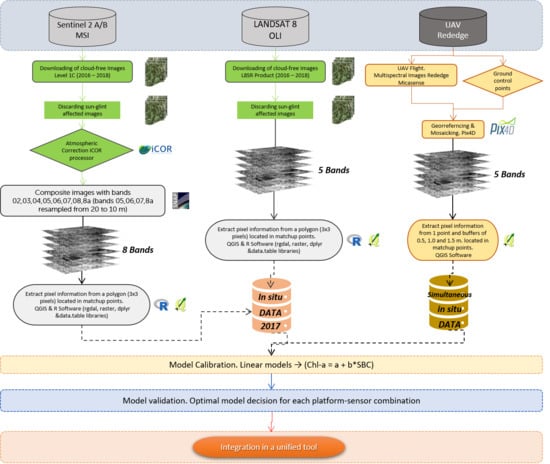
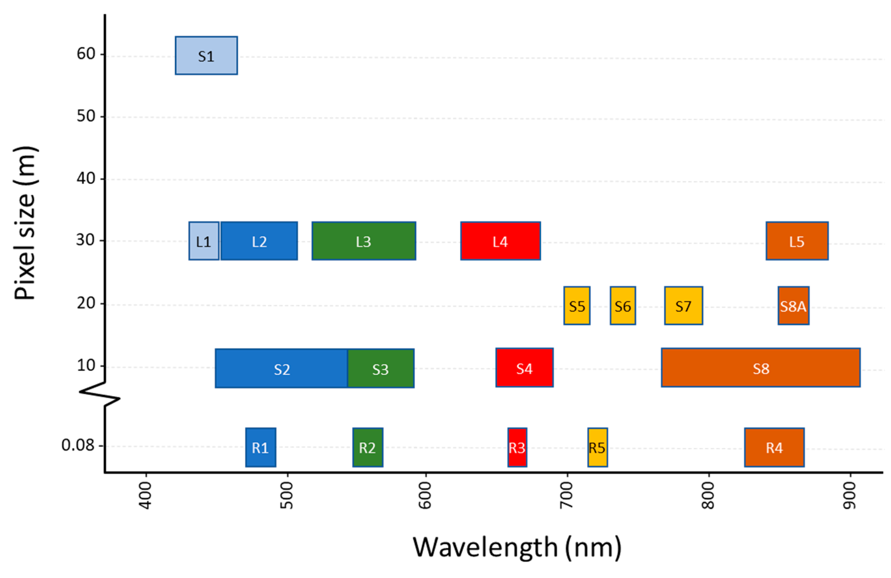
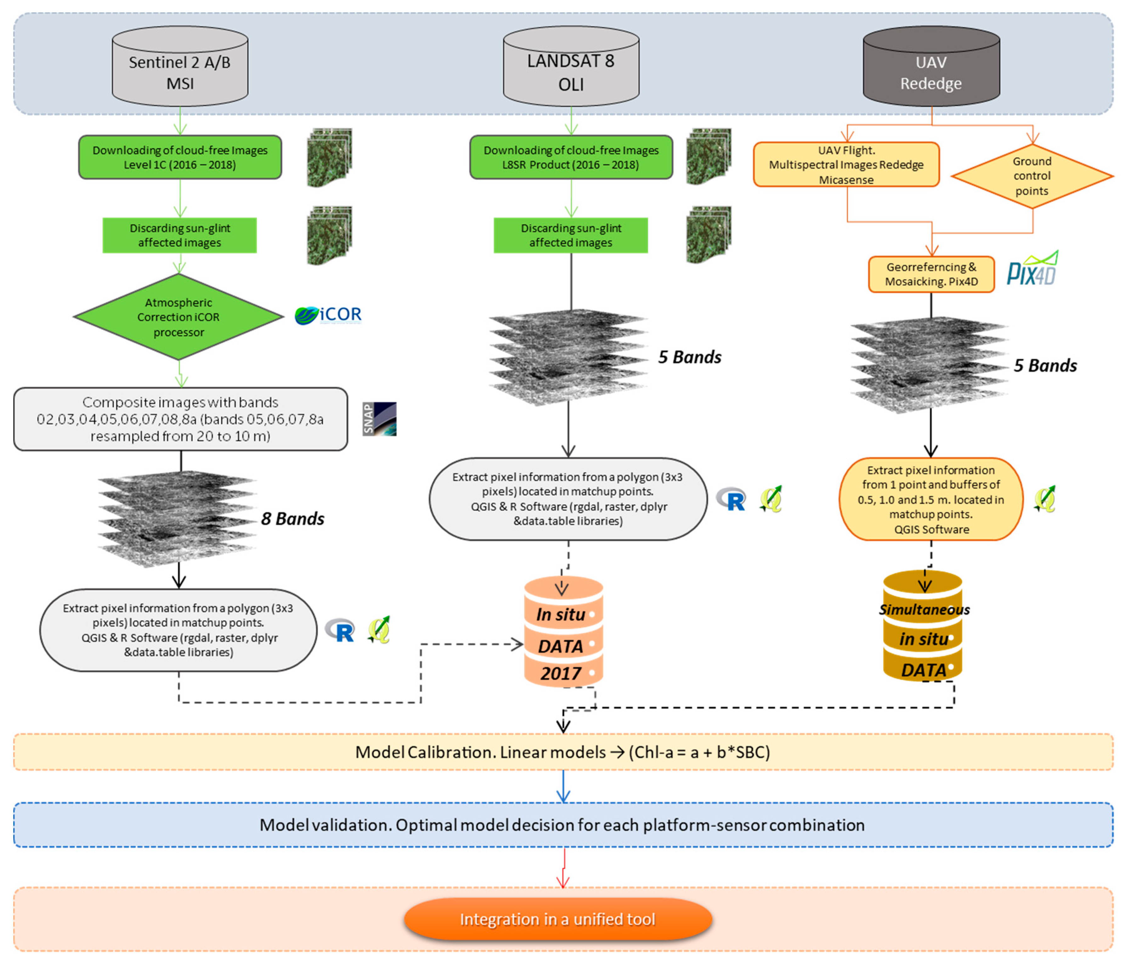
Based on this background, we propose a methodology for the monitoring of aquatic resources trying to maximize the periodicity of data acquisition and gap-filling by combining sensors and platforms, complementing an established monitoring program. On it, freely distributed images obtained through multispectral sensors on board two satellite platforms (Sentinel 2 and Landsat 8), used as a virtual constellation [25,26], are combined with commercial multispectral sensors mounted on UAV platforms. This approach is seeking to combine the affordability, stability, quality and continuity of ESA and NASA missions with the flexibility and spatial resolution provided by the use of UAV platforms, to make the most of these resources in favor of efficient management of aquatic resources. The empirical approach has been used to test the retrieval of chl-a as a quantitative descriptor of the presence of phytoplankton and the degree of eutrophication of a small water body, using images at different scales taken with three multispectral sensors with different characteristics, in a test carried out during 2017 and 2018 in a drinking water reservoir regularly affected by the presence of cyanobacteria.

The objectives of the study are: (1) To evaluate the performance of different algorithms and band indices in a small waterbody, by using images obtained with three different sensors, during 2016, 2017 and 2018. (2) To validate the application of free-distributed multispectral images from Sentinel 2 and Landsat 8 satellites to improve the continuous monitoring of small reservoirs, in an area of very high cloud cover (Galicia, NW Iberian Peninsula). (3) To assess the detection and quantification capability for chl-a of a remote sensing system consisting of a commercial multispectral camera on board a multirotor UAV and to verify its potential application in the absence of valid satellite images.

2. Materials and Methods

2.1. Study Area

The study area is a small reservoir (4.5 ha) with a capacity of 0.24 hm³ located in Spain, in the northwest (NW) of the Iberian Peninsula (Figure 1). Since 2000, the reservoir has maintained a drinking water supply service for households and facilities in the municipality. According to the data obtained during the conducted sampling, it has a maximum depth of 9.0 m. A river park was set up in 2012, when the reservoir also became navigable and a small jetty and a recreational area were installed, confirming its use as a leisure area for residents. The reservoir is located in the Atlantic Biogeographical Region, under an oceanic temperate climate, with a mean annual temperature of 19.6 °C and high precipitation (1146.2 mm) and relative humidity (90.6%) (mean annual values for five years (2013–2017) [27]). The rainiest period spans from November to February.

The main problem facing the reservoir is eutrophication. It has a very small catchment area with agricultural and livestock farms that, in many cases, generate an excess of slurry responsible for the existence of diffuse organic pollution and an excess of nutrients in the water. It is a system affected by recurrent cyanobacterial blooms with periodic high chl-a concentration, especially in late summer-early autumn (

Table 1. Summary statistics of the chl-a values (μgr/L) registered in the two sampling points of the reservoir during the periodic monitoring during the 3 years of the study period. (n is the total number of samples available for each year and sample point BC and BP). Source: [28].

	BC					BP
	Mean	Min	Max	SD	n	Mean	Min	Max	SD	n
2016	26.01	6.29	134.34	27.14	22	314.49	2.42	1779.57	574.77	12
2017	11.11	3.09	21.16	4.76	45	20.96	2.86	89.70	18.75	43
2018	64.47	2.40	1028.76	216.23	23	130.31	2.65	1353.66	339.85	22

), documented by the Environmental Information Service of Galicia (SIAM) since 2012 (www.siam.xunta.gal). In addition, its proximity to a highway makes it sensitive to potential spills from it. Taking this into account, and the sensitivity due to its role as the supply of drinking water and a leisure and recreational area, this reservoir is considered a very good example of a system with the need for preventive monitoring and periodic control.

2.2. In Situ Data

The in situ chl-a data used to calibrate and validate the satellite models were taken from the Galician Platform for Environmental Information (GAIA), supplied freely and on a regular basis, coming from the cyanobacterial monitoring program in the reservoirs of the district [28]. It maintains 2 permanent sampling points in the waterbody, one close to the dock (BP) and the other near the uptake system for drinking water (BC) (Figure 1). For the purpose of this study, we established two matchup points for the satellite reflectance data retrieval, as near as possible as these two ones, in a place still considered representative of the chl-a values, while far enough from the dock and the wall dam to be as unaffected as possible from adjacency effects. The point near the dock (BP) is located in the direction of dominant winds and tends to accumulate a high concentration of cyanobacteria during bloom events. Under such conditions, this point was not considered representative of the free water pixel used for matchup with satellite images and not used in the study.

Chl-a concentrations were retrieved from filtered surface water samples followed by acetone extraction and fluorometric measurements [29]. All the samples were taken from 10:00 am to 2:00 pm (local time). The sampling period used for calibration spans from January 2017 to December 2017, with a dataset of 45 samplings and 86 potential matchup points. The available data for validation is from the previous and following year: 2016 (from 4th January to 19th December) and 2018 (5th March to 26th November) with a dataset of 34 and 45 potential matchups, respectively.

During the field data campaigns, simultaneously to the UAV flights (19th September 2017 and 2th October 2018), water samples were also taken in 5 points of the reservoir (Figure 1). As the 90% of the radiation received by the remote sensors comes from the first optical thickness, which corresponds to 0.6 times the Secchi disk depth (SD) ([24,30], integrated water samples were taken with a hosepipe from the surface layer at a depth equal to 0,6*SD. These water samples were then taken to the lab, stored in the dark in a cooler and analyzed for chlorophyll a (chl-a), phycocyanin (PC), Total Suspended Solids (TSS) and Dissolved Organic Carbon (DOC). The chl-a was determined by acetone extraction (90%) followed by spectrophotometric measurements and the application of Jeffrey and Humpfrey [31] equations following the procedure described in [32]. Phycocyanin determination was made by the method described by Quesada [33]. The method for obtaining TSS was nº2540D of the APHA Standard Methods [32] and the DOC concentration was obtained through combustion and catalytic oxidation followed by NIR with a Skalar Formacs HT TOC analyzer following UNE EN 1484:1998.

Five profiles were also done with a YSI6600 multi parameter sonde with the following attached sensors: temperature (°C), electrical conductivity (µS/cm.), pH/ORP, dissolved oxygen (% and mg/L), turbidity (NTU), chlorophyll (µgr/L) and phycocyanin (BGA-PC, cells/mL). The sample taken in the central point of the reservoir was also analyzed for principal nutrients (Total Phosphorous TP, Total Nitrogen TN, Nitrate, Nitrite and Ammonium). TP was analyzed by ICP-MS following an internal procedure of the support services for research (SAI) of the University of A Coruña (nº P-SAI-UEPM-09) accredited by ENAC, with high-resolution equipment (ELEMENTXR/ELEMENT2; Thermo Finnigan). Determination of TN was done through catalytic combustion and chemiluminiscence detection following prior oxidation with a Skalar Formacs HT analyzer in samples filtered through membrane (Millipore Millex-HM, 0.45 µm) following UNE-EN 12260:2004. Colorimetric ammonium determination was performed by AquaKem 250 (Labmedics) in water samples previously filtered through Millex-HN membrane (0.45 µm) following SAI internal procedure: P-SAI-UAA-15. Nitrate and nitrite were determined by ionic chromatography with a chromatographer Metrohm 850 Professional IC equipped with a column Metrohm Metrosep A Supp 7 250/4.0 mm, following the internal SAI procedure: P-SAIUAA-20.

2.3. Remotely Sensed Data

Three different multispectral sensors on board four platforms were used as well as three satellite platforms (S2A, S2B and L8) and one UAV platform (Octocopter Atyges FV8). The characteristics (spatial resolution and bandwidths) of the sensors (namely MSI, OLI and Rededge Micasense) are described in Figure 2 and

Table 2. Bandwidths, central wavelengths (nm) and spatial resolution (m) of the evaluated sensors bands. In case of MSI Sentinel 2A data are given.

L8 OLI.	B1	B2	B3	B4					B5
Bandwidth	20	65	75	50					40
Central wavelength	443	482	562	655					865
Resolution.	30	30	30	30					30
S2A MSI	B1	B2	B3	B4	B5	B6	B7	B8	B8a
Bandwidth	21	66	36	31	15	15	20	106	21
Central wavelength	443	492	560	665	704	740	783	833	865
Resolution.	60	10	10	10	20	20	20	10	20
Rededge Mic.		B1	B2	B3	B5			B4
Bandwidth		20	20	10	10			40
Central wavelength		475	560	668	717			840
Resolution.	0.08

).

2.3.1. Satellite Imagery Pre-Processing

All available images of both sensors (MSI and OLI) acquired during 2017 were considered for calibration. The first selection criterion was a maximum interval of 3 days with respect to the acquisition of in situ data. Images with cloud cover were discarded, achieving a final number of 21 a priori valid images for Sentinel 2A and 2B. Once processed and analyzed, those images taken during winter (December, January and February) were considered not valid because of the shadow projected from the hills besides the reservoir. The imagery of the rest of the year, captured under higher sun elevation angles, were not affected by this artifact. The final number of Sentinel 2 MSI valid images for 2017 were 12 (24 potential matchups). Landsat 8 OLI images were obtained following the same criteria as for Sentinel 2, with a final number of 7 valid scenes for calibration (14 matchup points).

The validation dataset with the previous and following year images (2016 and 2018) followed the same rules. For Sentinel 2 MSI, 4 images of 2016 and 7 images of 2018 were considered valid. The 2016 dataset has few images because only S2A was operational and the high cloud cover in this area; moreover, some of the cloud-free images were invalid by a very strong sun-glint effect. The S2 MSI validation dataset was made of 15 match-up points. In case of Landsat 8, the validation dataset was made of 5 images of 2016 and 6 corresponding to 2018, with a total number of 14 match-up points.

The Sentinel 2 MSI product used was L1C scenes in the SAFE format, i.e., orthorectified, geolocated and radiometrically calibrated top-of-atmosphere (TOA) reflectances in Universal Transverse Mercator (UTM) projection with the WGS84 datum. S2 MSI images were subsequently corrected to bottom-of-atmosphere (BOA) reflectance using the iCOR (Image Correction for atmospheric effects) atmospheric correction algorithm (AC processor), a single atmospheric correction implementation for land and water. It derives aerosol optical thickness from the image and allows for adjacency correction with SIMilarity Environmental Correction (SIMEC) over water. In iCOR, land pixels are used to derive the AOT based on an adapted version of the SCAPE-M method and uses MODTRAN5 LUT to perform the atmospheric correction. Solar and viewing angles (Sun zenith angle (SZA), view zenith angle (VZA) and relative azimuth angle (RAA)) and a DEM are used as auxiliary data and can originate from external sources or be derived from the image itself [34]. Default settings for this processor were used and the SIMEC option was enabled. iCOR is implemented as a plugin in the SNAP (Sentinel Application Platform) toolbox version 6.0. Once atmospherically corrected, all the used spectral bands were resampled to a 10-m. pixel size by the nearest neighbor resampling method in SNAP 6.0.

The Landsat 8 OLI product used was Landsat 8 Surface Reflectance (L8SR). The L8SR product [35] is processed with the LaSRC algorithm and made available by the United States Geological Survey (USGS). The images are radiometrically calibrated and orthorectified, projected in Universal Transverse Mercator (UTM) with the WGS84 datum. The L8SR product provides the surface reflectance image rescaled by a factor of 10,000. This product has been proven effective in aquatic applications [36,37,38]. For both satellite products, surface reflectance data were transformed into Rrs dividing by π.

The extraction of the pixel information from 30 × 30 m. polygons (3 × 3 pixels for Sentinel 2 and 1 pixel for Landsat 8) located in matchup points, was done using QGIS and R software (rgdal, raster, dplyr and data.table libraries [39,40,41,42,43]) (see Figure 3).

2.3.2. UAV Imagery Pre-Processing

In order to increase the spatial and temporal resolution obtained with freely available satellite imagery, a complementary system was implemented based on the analysis of multispectral images taken with a commercial sensor (Rededge Micasense) (5 bands; Figure 2, Table 2) on board an octocopter (Atyges FV8). The first sampling took place on 19/09/2017and a second one, with the initial objective of model validation, was done during the same phenological period in 2018 (2th October).

The flights time was 12:00 am, established regarding the sun angle (between 30° and 60° to minimize sun-glint effects and specular reflections). Nine ground control points were distributed evenly in the flight area and x,y,z coordinates were surveyed with a GPS with submetric precision. The flight mission was planned as a simple grid with a distance between flight lines of 45 m. and a flight height of 120 m; the speed of the octocopter was set to 4 m/s.

No atmospheric correction was applied on the UAV imagery, as there were still not commercially available atmospheric corrections designed for aquatic purposes and UAV close-range remote sensing. Besides, the purpose of this work was to deliver an operational solution with no dependencies on concurrent field radiometric sampling, and therefore the effect of the thin atmosphere layer between the sensor and the water surface was neglected. The georeferencing, radiometric processing and mosaicking of the image were performed with the Pix4D software (Pix4D, Lausanne, Sw.). Raw multispectral images were corrected to ground absolute reflectance using the irradiance measures taken along with each snapshot by a specific sensor onboard the UAV and spectrally rescaled against a calibration panel with values around 70 % of diffuse reflectance in the visible-infrared spectrum. The extraction of the image information was done at different sampling sizes corresponding to the median of all the pixel values included in circular buffers of 0.5, 1.0 and 1.5 m. around each match-up point using QGIS 2.18.15. These buffers were set in order to test the coherence and representativeness of the data given by the sensor against a different size of sampling areas around the in situ sampling points.

In order to compare the reflectances recorded by the S2 MSI and UAV sensors, we used two simultaneous images of both sensors (10/02/2018). We made a focal analysis on the Micasense bands in which the extent of each of the S2 MSI pixels covering the reservoir was used as focal unit, once filtered those prone to spectral mixtures from the shore area. From these extents (squares of 10 × 10 m. labelled with an unique ID), a synthetic value of the Micasense reflectance for each band was calculated as the mean value of the Micasense image pixels covered by the area of each individual S2 MSI image pixel extent.

2.3.3. Data Analysis

For developing the empirical model, linear fits were applied expressing the relationships between Rrs at different wavelengths in every match-up point and their corresponding “in situ” chl-a data as a linear function of the format:

chl-a = a + b × SBC

(1)

where a and b are the model parameters (intercept and slope, respectively) and SBC is the tested Spectral Band Combination (

Table 3. SBC adapted to the OLI, MSI and Rededge sensors on board Landsat 8, Sentinel 2 and UAV platforms.

Algorithm	Band Math L8 OLI	Band Math S2 MSI	Band Math Rededge	Reference
Kab 1 (Rrs)	1.67−3.94*ln(B2) +3.78*ln(B3)	1.67−3.94*ln(B2) +3.78*ln(B3)	1.67−3.94*ln(B1) +3.78*ln(B2)	[47]
Kab 2 (Rrs)	6.92274−5.7581*(ln(B1)/ln(B3)			[47]
SABI	(B5−B4)/(B2+B3)	(B8A−B4)/(B2+B3)	(B4−B3)/(B1+B2)	[48]
KIVU	(B2−B4)/B3	(B2−B4)/B3	(B1−B3)/B2	[49]
NDCI		(B5−B4)/(B5+B4)	(B5−B3)/(B5+B3)	[50]
NDVI	(B5−B4)/(B5+B4)		(B4−B3)/(B4+B3)	[50]
2BDA_1	B5/B4	B6/B4	B4/B3	[22]
2BDA_2		B7/B4	B5/B3	[22]
3BDA_1		(B4−1 − B5−1) * B6	(B3−1 − B5−1) * B4	[21]
3BDA_2		(B4−1−B5−1)*B7		[21]
3BDA_MOD			(B3−1−B5−1)
B3B1	(B3−B1)/(B3+B1)		(B2−B1)/(B2+B1)	Normalized indices
B3B2	(B3−B2)/(B3+B2)	(B3−B2)/(B3+B2)
GB1	B3/B1		B2/B1	Simple ratio
GB2	B3/B2	B3/B2		Simple ratio
GR	B3/B4	B3/B4	B2/B3	Simple ratio

). SBCs are either an index, a ratio or an algorithm. Some of these combinations (of two and three bands) are those proposed by different authors and adapted to OLI, MSI and Rededge spectral bands (Figure 2, Table 2).

As shown in Table 3, in addition to the standard 3 bands and 2 bands algorithms (3BDA and 2BDA) [21,22], we have included one modification of the 3 bands algorithm (3BDA_MOD) adapted to UAV- Rededge Micasense data.

These both algorithms (2BDA and 3BDA) come from a common initial conceptual model, relating remotely sensed reflectance and pigment content in vascular plant leaves [44]. The model was initially conceived to isolate the absorption coefficient of the pigment of interest from the reflectance spectrum. The 3BDA relationship used between the pigment content in the leaves and the reflectance was as follows:

$$3BDA-Pigmentconcentration\propto \left(R_{\lambda 1}^{-1}-R_{\lambda 2}^{-1}\right)R_{\lambda 3}$$

(2)

When the 3BDA model is tuned for the retrieval of chl-a in turbid productive waters, as described by [21,22,45], the spectral regions are defined as:

• λ₁: Spectral region such that R⁻¹_λ1 is maximally sensitive to the absorption chl-a but still affected by the absorption of other constituents and backscattering: λ₁ = 660–690 nm.
• λ₂: Spectral region such that R⁻¹_λ2 is minimally sensitive to chl-a for which the absorption by other constituents is almost equal to that at λ₁: 710-λ₂-730 nm.
• λ₃: Spectral region minimally affected by the absorption of pigments, used to compensate for the variability in backscattering between samples: initially λ₃ > 740 nm.

The 2BDA algorithm is described by the authors as a particular case of the 3BDA, which only uses the λ₁ and λ₃ terms of the equation and gives good results when a_chla(λ₁) ≫ b_b and a_chla(λ₁) ≫ a_tripton(λ₁)+ a_CDOM(λ₁) [39], any a being the absorption coefficients and b_b the backscattering coefficient.

$$2BDA-Pigmentconcentration\propto \left(R_{\lambda 1}^{-1}\right)R_{\lambda 3}$$

(3)

Two formulations for Sentinel 2 MSI data were tested for 2BDA and 3BDA, using Rrs from Bands 6 and 7 as R_λ3. Band 6 Rrs data for MSI have been mostly used in 3BDA and 2BDA algorithms formulated by other authors (e.g., [46]) as it offers more reliable data for water studies inside the NIR region of the spectrum than the rest of NIR bands in MSI. Yet, this band is centered exactly in 740 nm, which is lower than the theoretical wavelength specified by [23] who established the optimal wavelength above 740 nm and obtained the best results with 740–750 nm. Therefore, just one version of these two algorithms with Rrs data from Band 7 (Figure 2, Table 2 and Table 3) was tested.

The computation (R⁻¹ λ₁ - R⁻¹ λ₂) is related to the content of chl-a, but it is still affected by the variability in the backscattering of the medium; however, in our case, we also tried to apply this part of the algorithm alone with the UAV Multispectral Imagery data.

Other algorithms using red and NIR bands were tested, like the Normalized Difference Chlorophyll Index (NDCI) [50] and the Normalized Difference Vegetation Index (NDVI). The first one was inspired in NDVI and developed to retrieve chl-a emulating MERIS channels, thus using Rrs (708) and Rrs (665). NDVI was used in case of L8 OLI images in our study in absence of 708 nm band in this sensor, and also tested for Rededge Micasense.

Algorithms and indices using known features in blue and green spectral channels were also evaluated. We can divide them into two groups.

The first group used green and blue bands but also red and/or NIR. In this group, we have tested Surface Algal Bloom Index (SABI) [48] initially defined with MODIS bands to delineate the spatial distribution of floating micro-algal species in ocean waters with a NIR response similar to that of land vegetation, using in this case MODIS Rrs (869 nm) as NIR data. KIVU, developed for a freshwater lake with chl-a values below 6 μgr/L using Landsat 5 TM images [49], is also in this group. This algorithm uses blue and green bands (TM1 and TM2) and also the red band (TM3) to correct for the additional radiance caused by the scattering of non-organic suspended matter (see Table 3 for formulation and references).

In the last group, we tested Kab1 and Kab2, algorithms developed including blue and green bands and originally formulated for coastal areas using Landsat 7 ETM+ bands. Finally, in this group, we also tested simple ratios (GB1, GB2) and normalized indices (B3B1, B3B2) using only the green and blue bands available for each sensor.

Linear fits were adjusted both to chl-a data and Ln (chl-a) data, this approach also being tested by other authors to account for the non-normal distribution of the chl-a values [47,51].

The validation of the best performing models was done, only in case of satellite data, with images of the previous and next years (2016 and 2018). For both years, the validation was done with data in the chl-a range of 1–40 µgr/L for which the models were calibrated. A range of 4.38–20.42 µgr/L was used in case of Landsat 8 OLI, and 4.38–34.64 µgr/L in case of Sentinel 2 MSI.

The statistical metrics used for the validation exercise were: Root Mean Square Error (RMSE, Equation (4)), Normalized Root Mean Square Error (NRMSE, Equation (5)), Mean Absolute Percentage Error (MAPE, Equation (6)) and bias (Equation (7)).

$$RMSE=\sqrt{1/n{{\displaystyle \sum }}_{i=1}^n{\left(y_{pi}-y_{mi}\right)}^2},$$

(4)

$$NRMSE=\frac{RMSE}{y_{mmax}-y_{mmin}},$$

(5)

$$MAPE=\frac{1}{n}{\displaystyle \sum }_{i=1}^n\left(\frac{\left|y_{pi}-y_{mi}\right|}{y_{mi}}\right)$$

(6)

$$bias=\frac{1}{n}{{\displaystyle \sum }}_{i=1}^n\left(y_{pi}-y_{mi}\right),$$

(7)

where $y_p$ is the predicted values, $y_m$ is the measured values and n is the number of samples.

3. Results

3.1. Water Quality

The studied reservoir is an eutrophic waterbody with recurrent cyanobacterial blooms since 2012, documented through the Galician Platform for Environmental Information (GAIA) (www.gaia.xunta.es) (Table 1). This periodic monitoring showed during 2017 Microcystis sp. as the dominant cyanobacteria, even though Chorococcus sp., Aphanocapsa sp. and Woronischia sp. were also present. The chl-a reached a maximum in the BC point (which is considered more representative of the main waterbody) of 21.26 µgr/L during May being the mean value for this year in BC sampling point 11.11 µgr/L. The highest cyanobacteria cell concentration was registered in October (9750 cel/mL) being Aphanocapsa sp. the dominant taxa. In the BP sampling point, the maximum chl-a was registered on 25th September (89.70 µgr/L), in this case, Microcystis sp. Being the dominant cyanobacterial taxa (115,500 cel/mL), and the mean annual value 20.96 µgr/L [28]. During 2018 (when the second UAV flight was done) the general condition of the reservoir was very different, with bigger cyanobacterial blooms, the mean and maximum values of chl-a being higher than in 2017 (BCmean = 64.47 µgr/L, BPmean = 130.31 µgr/L). This documented highly changing condition in space and time makes this drinking water reservoir a suitable example of a sensible area which needs to be continuously monitored (Table 1).

The water sampling (5 sampling points) made synchronous with the first UAV flight (19th September 2017) showed a situation of low nutrient concentration and phytoplankton biomass (low both chl-a and PC), even though the Secchi Depth values together with turbidity and TSS indicate a slightly turbid state (

Table 4. Summary of the water analysis results of the in situ samplings synchronous with the UAV flights (DOC: Dissolved Organic Carbon; TSS: Total Suspended Solids; EC: Electrical Conductivity, P total: Total Phosphorous).

	2017			2018
	Mean	Max	Min	Mean	Max	Min
Chlorophyll a (µgr/L)	2.19	2.68	1.34	93.04	99.3	89.84
Phycocyanin (µgr/L)	0.18	0.24	0.13	19.03	27.21	18.86
Turbidity (NTU)	4.16	5.20	3.07	2.3	2.8	1.4
Sechi Disc Depth (m.)	1.7	2.0	1.5	1.6	1.75	1.20
pH Surface	7.18	7.26	7.04	7.22	7.32	7.08
DOC (mg/L)	2.22	2.10	2.40	2.77	2.99	2.57
TSS (mg/L)	3.20	6.8	1.2	21.5	27.2	18.0
OD sup (mg/L)	9.72	9.90	9.47	10.5	10.71	10.36
Temp surface (°C)	16.83	16.87	16.76	16.33	16.43	16.15
EC surface (µS/cm)	129.6	131.0	128.0	127.0	127.0	127.0
P total (mg/L)	0.021			0.013
Ammonium (mg/L)	< 0.05
Nitrite (mg/L)	0.057
Nitrate (mg/L)	9.27
N total (mg/L)	2.20			2.76

).

Even though the phenological phase was considered the same in 2018 and in 2017, the second UAV flight was done in very different water quality conditions with a cyanobacterial bloom in the reservoir and much higher chl-a and PC concentrations (Table 4). Curiously, turbidity was higher in the first flight. Even though the same number of samples (5) was taken in either campaign, we have 4 data in 2018 as one of the chl-a samples had to be discarded.

3.2. Spectral Band Combinations for the Retrieval of chl-a

The empirical approach was selected to build models for the retrieving of chl-a from the three types of multispectral images. All the indices and band ratios tested were adapted to the characteristics of the bands of each sensor (Table 2 and Table 3, Figure 2). In case of satellite imagery, the time window used for the development of the algorithms (3 days) can be a source of error in case of sudden changes in the development of an algal bloom. The chosen year for the calibration of the models was the one with more potential matchups (more in situ data) and stable conditions regarding chl-a concentration (cf. Table 1), in order to reduce the uncertainty in the calibration of the models regarding this time difference. To evaluate this effect, we plotted the scatter plot graphics for the calibrated models for retrieving chl-a with a color code reflecting this time difference (0–3 days) (e.g., Figure 4F).

3.2.1. Landsat 8 Imagery

In the calibration to find a suitable linear model for the determination of chl-a (Equation (1)) with Landsat 8 OLI multispectral data, most of the algorithms and band indices tested were positive and significatively correlated (Pearson correlation) with chl-a concentration (

Table 5. Linear model coefficients and linear fit parameters for all the Spectral Band Combinations (SBC) tested for the retrieval of chl-a with multispectral Landsat 8 OLI data. The models were done with Ln (Chl-a). n = 13.

SBC	Intercept (a)	Slope (b)	R2	Pearson r	p Value	Sig. Code 1
SABI	1.979	0.575	0.750	0.866	0.0001	****
KIVU	2.084	−1.127	0.504	−0.710	0.0066	***
NDVI	1.923	1.448	0.749	0.865	0.0001	***
2BDA	1.619	0.350	0.764	0.874	0.0001	****
Kab 1	1.534	0.177	0.636	0.797	0.0011	***
Kab 2	2.797	−0.590	0.403	−0.635	0.0198	**
B3B1	2.077	0.961	0.479	0.692	0.0087	***
B3B2	2.020	1.654	0.615	0.784	0.0015	***
GB1	2.083	0.122	0.233	0.483	0.0945	*
GB2	1.521	0.517	0.577	0.759	0.0026	**
GR	1.622	0.681	0.082	0.286	0.3431

¹ (*) p < 0.1; (**) p < 0.05; (***) p < 0.01; (****) p < 0.001.

). The linear fit was made with both chl-a data inside an interval of 5.65–18.09 µgr/L, and Ln transformed chl-a data, giving the latter the best results.

Given the inherent complexity of inland waters, the combinations using red and NIR bands, specifically 2BDA, SABI and NDVI, were the best performing Spectral Band Combinations. The Surface Algal Bloom Index (SABI) which uses green and blue bands in addition to red and NIR [48] also gave good results. These three had the strongest (Pearson r > 0.8) and the more significative correlations with Ln(chl-a) data (Table 5, Figure 4). The results obtained with un-transformed Ln data did not show high differences, the Pearson r and R² being 0.858 and 0.753 for 2BDA, 0.844 and 0.712 for SABI and 0.834 and 0.6953 for NDVI models, respectively. Kab_1 was also tested as its results were considered good, but the scatterplot showed a relationship based in two defined and separated group of points.

Chl-a models fitted for the 2017 data were subsequently applied to Landsat 8 OLI datasets from 2016 and 2018. The validation, with chl-a from 4.38 to 20.42 µgr/L, showed very similar results for the three best performing indices (Figure 5,

Table 6. Model validation metrics for the best performing models with Landsat 8 OLI.

	RMSE	NRMSE	MAPE	Bias
LANDSAT 8 OLI
SABI	6.30	39.28	69.90	0.94
2BDA	6.46	40.25	65.69	1.07
NDVI	6.26	39.05	65.83	1.13
Kab_1	5.47	34.99	57.26	−0.02

). However, all showed a tendency to overestimate chl-a values (bias ranging from 0.94 to 1.13). The lowest root mean square error (RMSE) was obtained with the NDVI index, which also gave the lowest NRMSE and MAPE, very similar to 2BDA, but the highest bias. Despite the good results in the calibration, the validation did not show a good agreement between measured and predicted values. Even though Kab_1 validation metrics were better that the other models, the graphical output, both for the calibration and the validation, shows a weaker performance (Figure 5, Table 6).

3.2.2. Sentinel 2 Imagery

In the calibration of linear models with Sentinel 2 MSI data, the number of significative correlations with the Spectral Band Combinations was less than for OLI data; the relationships were also slightly weaker. Still, 5 of them were strong, with a Pearson correlation coefficient above 0.7 and the highest significance level. In this case, the best fits were obtained with the chl-a value, and not with the Ln transformed data. The chl-a values in this case ranged from 5.09 to 50.37 µgr/L.

As with OLI data, all the linear models with Pearson r > 0.8 and a p value lower than 0.0001 were considered the best performing and were tested in the validation stage. In this case, we also included in the validation the 3BDA algorithm, as it also gave good results and the correlation coefficient was close to 0.8 (Table 6). In case of Sentinel 2 data, not only did the combination of the NIR and red bands fit best with chl-a values but also 3 Spectral Band Combinations with green and blue bands gave similarly good results (

Table 7. Linear model coefficients and linear fit parameters for all the Spectral Band Combinations tested for the retrieval of chl-a with multispectral Sentinel 2 MSI data. The models were done with in situ chl-a. n = 23.

Index	Intercept (a)	Slope (b)	R2	Pearson r	p Value	Sig. Code 1
SABI	5.885	31.716	0.112	0.335	0.1274
KIVU	24.360	−28.930	0.296	−0.544	0.0089	***
NDCI	10.130	61.300	0.213	0.461	0.0306	**
2BDA_1	29.516	−9.168	0.174	−0.417	0.0532	*
2BDA_2	−30.740	22.850	0.702	0.837	0.0000	****
3BDA_1	14.515	3.597	0.006	0.081	0.7203
3BDA_2	7.134	26.795	0.532	0.729	0.0001	****
Kab_1	−5.064	6.361	0.679	0.824	0.0000	****
B3B2	8.662	61.763	0.673	0.820	0.0000	****
GB2	1.611	10.119	0.656	0.810	0.0000	****
GR	2.766	6.108	0.073	0.270	0.2234

¹ (*) p < 0.1; (**) p < 0.05; (***) p < 0.01; (****) p < 0.001.

, Figure 6).

The results obtained in the linear fits with Ln transformed data showed a lower performance in case of Sentinel 2, the Pearson r and R² being 0.718 and 0.5167 for 2BDA_2, 0.660 and 0.436 for 3BDA_2, 0.653 and 0.427 for Kab_1 and 0.659 and 0.435 for B3B2, respectively.

As can be seen in Figure 6, the models using blue and green bands (Kab_1, B3B2) gave relatively high R² values but the correlation was highly dependent on one data point, so they were not considered robust. The results of the calibration/validation exercise are given (

Table 8. Model validation metrics for the best performing models with Sentinel 2 MSI.

	RMSE	NRMSE	MAPE	Bias
SENTINEL 2 MSI
3BDA_2	4.44	14.67	41.17	0.25
2BDA_2	7.94	26.24	87.18	−0.94
B3B2	10.22	33.76	106.33	3.44
Kab_1	9.36	30.93	99.81	2.71
GB2	8.94	29.55	93.80	2.11

, Figure 7).

The validation of these models was done, as with OLI data, with the valid images for the previous and following years (2016 and 2018) and a chl-a interval from 4.38 to 34.64 µgr/L. The validation metrics showed different performances for these 5 models (Table 8). 2BDA tended to underestimate the chl-a values, giving even negative results (Figure 7), while 3BDA showed a positive bias of 0.25. All indices with good performance in calibration using blue and green bands (B3B2, Kab_1 and GB2) tended to greatly overestimate the chl-a concentration. The best model regarding the validation results for Sentinel 2 MSI was the one using 3BDA algorithm and Band 7 Rrs as the NIR data input, with the lowest values for all metrics, followed by 2BDA, as can also be seen in the validation scatterplots (Figure 7)

A clear pattern regarding the influence of the time window in the calibration of the algorithms (Figure 4 and Figure 6) could not be found in the graphical analysis for Sentinel 2 but Landsat 8 graphics showed the worst fit for the 3-day time-lapse points. Overall, once the validation was done, the best performing model for retrieving chl-a in the studied reservoir was the one fitted with the 3BDA algorithm applied to Sentinel 2 imagery. The validation results for Landsat 8 were poorer than Sentinel 2.

3.2.3. UAV Imagery. Model Calibration

The two UAV flights (2017 and 2018) were made in late summer-early autumn, when the cyanobacterial bloom events take place in this area. This sampling plan was intended to calibrate and subsequently validate the models; but two opposite conditions of algal bloom development were found (extremely different chl-a values, cf. Table 4). The chl-a interval covered was too broad to validate the models obtained with the 2017 flight with the data of the 2018 flight, so the validation was not possible. Nevertheless, these two opposite situations gave the opportunity to test the multispectral sensor performance in low and high chl-a concentrations, test the coherence of the relationships between flights and to test which of the Spectral Band Combinations were most “portable” to monitor chl-a concentration in waterbodies with different eutrophication levels.

The 2017 flight, done in low chl-a concentration conditions, showed a better performance of the Spectral Band Combinations using NIR and red bands. Even though some positive correlations were found, the only significative one applies a modified version of the 3BDA model (3BDA__MOD), for all the three sampling areas tested. (

Table 9. Linear model coefficients and linear fit parameters for all the Spectral Band Combinations tested for the retrieval of chl-a with multispectral data from Rededge Micasense on board the UAV platform for the 2017 flight. The models were done with in situ chl-a and the median of the reflectance values included in a buffer of 0.5 m. around the sampling point.

Index	Interc. (a)	Slope (b)	R2	Pearson r	p Value	Sig. Code 1
SABI	2.073	3.085	0.264	0.514	0.3755
KIVU	3.665	−9.405	0.711	−0.843	0.0727	*
NDCI	4.091	28.404	0.603	0.776	0.1225
NDVI	2.088	2.778	0.363	0.603	0.2819
2BDA	0.970	1.109	0.267	0.517	0.3721
3BDA	3.262	7.039	0.046	0.215	0.7279
3BDA_MOD	3.715	0.2615	0.945	0.972	0.0055	***
2BDA_2	−12.031	16.256	0.597	0.773	0.1256
B3B1	1.371	9.470	0.037	0.193	0.7549
GB1	−2.578	4.008	0.038	0.195	0.7526

¹ (*) p < 0.1(**) p < 0.05; (***) p < 0.01; (****) p < 0.001.

,

Table 10. Linear model coefficients and linear fit parameters for all the Spectral Band Combinations tested for the retrieval of chl-a with multispectral data from Rededge Micasense on board the UAV platform for the 2017 flight. The models were done with in situ chl-a and the median of the reflectance values included in a buffer of 1.0 m. around the sampling point.

Index	Interc (a)	Slope (b)	R2	Pearson r	p Value	Sig. Code 1
SABI	2.083	3.132	0.266	0.515	0.3738
KIVU	3.708	−9.950	0.733	−0.856	0.0638	*
NDCI	4.124	28.100	0.527	0.726	0.1647
NDVI	2.100	−2.823	0.369	−0.607	0.2773
2BDA	0.940	1.1485	0.274	0.524	0.3648
3BDA	2.387	1.273	0.001	0.037	0.9521
3BDA_MOD	3.830	0.276	0.927	0.963	0.0085	***
2BDA_2	−11.787	16.039	0.520	0.721	0.1688
B3B1	1.599	6.787	0.020	0.143	0.8186
GB1	−1.242	2.881	0.021	0.145	0.8158

¹ (*) p < 0.1; (**) p < 0.05; (***) p < 0.01; (****) p < 0.001.

and

Table 11. Linear model coefficients and linear fit parameters for all the Spectral Band Combinations tested for the retrieval of chl-a with multispectral data from Rededge Micasense on board the UAV platform for the 2017 flight. The models were done with in situ chl-a and the median of the reflectance values included in a buffer of 1.5 m. around the sampling point.

Index	Interc. (a)	Slope (b)	R2	Pearson r	p Value	Sig. Code 1
SABI	2.078	3.499	0.300	0.547	0.3395
KIVU	3.696	−9.954	0.719	−0.848	0.0695	*
NDCI	4.217	28.646	0.601	0.775	0.1236
NDVI	2.099	−3.047	0.401	−0.633	0.2514
2BDA	0.791	1.292	0.311	0.558	0.3285
3BDA	2.743	3.462	0.017	0.130	0.8344
3BDA_MOD	3.803	0.264	0.946	0.972	0.0054	***
2BDA_2	−12.06	16.41	0.594	0.771	0.1272
B3B1	1.729	5.301	0.8504	0.117	0.8504
GB1	−0.514	2.271	0.014	0.120	0.8471

¹ (*) p < 0.1; (**) p < 0.05; (***) p < 0.01; (****) p < 0.001.

, Figure 8)

The second flight results, done in high chl-a concentration conditions, confirmed the combination of red and NIR bands as the most suitable for chl-a retrieval with the Rededge Micasense sensor. In this case, the best performing models were always 2BDA and SABI (Figure 8,

Table 12. Linear model coefficients and linear fit parameters for all the Spectral Band Combinations tested for the retrieval of chl-a with multispectral data from Rededge Micasense on board the UAV platform for the 2018 flight. The models were done with in situ Chl-a and the median of the reflectance values included in a buffer of 0.5 m. around the sampling point.

Index	Interc. (a)	Slope (b)	R2	Pearson r	p Value	Sig. Code 1
SABI	90.672	28.895	0.912	0.955	0.0449	**
KIVU	102.65	−80.314	0.912	−0.955	0.0445	**
NDCI	97.157	31.436	0.320	0.566	0.4335
NDVI	91.359	20.330	0.753	0.868	0.1319
2BDA	81.783	9.017	0.867	0.932	0.0684	*
3BDA	94.014	2.844	0.012	0.112	0.8875
3BDA_MOD	96.948	0.130	0.433	0.658	0.3413
2BDA_2	78.540	18.710	0.290	0.538	0.4613
B3B1	64.07	112.43	0.2172	0.466	0.534
GB1	41.240	30.550	0.210	0.459	0.5408

¹ (*) p < 0.1; (**) p < 0.05; (***) p < 0.01; (****) p < 0.001.

,

Table 13. Linear model coefficients and linear fit parameters for all the Spectral Band Combinations tested for the retrieval of chl-a with multispectral data from Rededge Micasense on board the UAV platform for the 2018 flight. The models were done with in situ Chl-a and the median of the reflectance values included in a buffer of 1.0 m. around the sampling point.

Index	Interc. (a)	Slope (b)	R2	Pearson r	p Value	Sig. Code 1
SABI	90.684	29.020	0.911	0.9542	0.0457	**
KIVU	102.671	−80.930	0.907	−0.952	0.0477	**
NDCI	96.906	29.599	0.288	0.536	0.4634
NDVI	91.375	20.373	0.752	0.867	0.1330
2BDA	81.747	9.068	0.865	0.930	0.0696	*
3BDA	93.583	1.587	0.004	0.064	0.9358
3BDA_MOD	93.837	0.127	0.410	0.640	0.3591
2BDA_2	79.550	17.390	0.256	0.506	0.4937
B3B1	68.00	97.26	0.1573	0.396	0.6033
GB1	48.590	26.230	0.151	0.388	0.6114

¹ (*) p < 0.1; (**) p < 0.05; (***) p < 0.01; (****) p < 0.001.

and

Table 14. Linear model coefficients and linear fit parameters for all the Spectral Band Combinations tested for the retrieval of chl-a with multispectral data from Rededge Micasense on board the UAV platform for the 2018 flight. The models were done with in situ Chl-a and the median of the reflectance values included in a buffer of 1.5 m. around the sampling point.

Index	Interc. (a)	Slope (b)	R2	Pearson r	p Value	Sig. Code 1
SABI	90.672	29.021	0.9099	0.9539	0.0461	**
KIVU	102.730	−81.120	0.9056	0.9516	0.0483	**
NDCI	97.096	31.118	0.308	0.5550	0.4450
NDVI	91.361	20.354	0.750	0.8660	0.1340
2BDA	81.740	9.060	0.8651	0.9301	0.0698	*
3BDA	93.810	2.270	0.0079	0.0891	0.9109
3BDA_MOD	96.936	0.1305	0.4257	0.6524	0.3475
2BDA_2	78.740	18.430	0.2772	0.5265	0.4735
B3B1	66.56	102.88	0.1709	0.4133	0.5867
GB1	45.950	27.790	0.1644	0.4054	0.5945

¹ (*) p < 0.1; (**) p < 0.05; (***) p < 0.01; (****) p < 0.001.

).

In another exercise, the data of both flights were analyzed together. We used the 9 available points (5 from 2017 and 4 for 2018) to calibrate linear models that could be adjusted to this broad range of chl-a concentrations. As it was assessed that the results were similar for the 3 buffers tested (Table 9, Table 10, Table 11, Table 12, Table 13 and Table 14), this exercise was done only with the 0.5-m. buffer data. Even though this uneven distribution of data is associated with a high level of uncertainty, we considered the obtained results promising and worthy of being shown.

The only band combinations that fitted in a linear model applied to this broad range of chl-a concentration were those using the first part of the visible spectrum (blue, green and red bands). The combination of these bands (blue-green and green-red) gave the results shown in

Table 15. Linear model coefficients and linear fit parameters for all the Spectral Band Combinations tested for the retrieval of chl-a with multispectral data from Rededge Micasense on board the UAV platform combining the data of 2017 and 2018 flights. The models were done with in situ chl-a and the median of the reflectance values included in a buffer of 0.5 m. around the sampling point.

Index	Interc. (a)	Slope (b)	R2	Pearson r	p Value	Sig. Code 1
SABI	36.210	1110.010	0.0658	0.2565	0.552
NDCI	1.447	−431.077	0.2879	−0.5365	0.1364
NDVI	38.470	71.950	0.0456	0.2137	0.5809
2BDA	−3.8180	39.805	0.0780	0.2793	0.4666
3BDA	−10.15	−222.900	0.4587	−0.6773	0.0450	**
3BDA_MOD	14.629	−1.686	0.4288	−0.6548	0.0550	*
2BDA_2	263.500	−266.00	0.2773	−0.5265	0.153
B3B1	−41.980	520.310	0.9816	0.9907	0.0000	****
GB1	−205.40	175.30	0.9779	0.9889	0.0000	****
GR	−168.90	120.00	0.8654	0.9302	0.0002	****

¹ (*) p < 0.1; (**) p < 0.05; (***) p < 0.01; (****) p < 0.001.

and Figure 9. It can be seen that this relationship is based upon two separate groups of points, so it is not considered good for directly retrieving absolute chl-a values accurately; however, the results suggested that it can be used to classify the pixels into broad chl-a categories or classes to which apply algorithms specific to this narrower chl-a range inside of each class. This is also a key issue when dealing with cyanobacterial blooms with a spatial patchy distribution in waterbodies, in order to spatially stratify the analyses.

As it is shown in Table 15 and Figure 9, the best results were obtained for a normalized index using blue and green bands (B3B1), which gave the highest correlation coefficient (Pearson r = 0.9907) and R² (0.9816) and the highest significance level.

Chl-a = (520.310 ∗ B3B1) − 41.980

(8)

With these first results, we designed a preliminary ensemble model that uses the B3B1 algorithm as the first to be applied to the obtained images to classify the pixels into broad ranges of chl-a content. In our case, we could establish only two classes, dividing them in the middle of our 2 datasets: Class 1: chl-a < 50 μgr/L and Class 2: chl-a > 50 μgr/L. Once the chl-a value for each pixel in the images is obtained using this algorithm and classified into these 2 classes, the calibrated algorithms for low and high chl-a is subsequently applied to each pixel. The results of the application of B3B1 algorithm are shown in Figure 10, and the subsequent application for low and high chl-a value algorithms is shown in Section 3.3.

As it is shown in Figure 10, the image of 2017 was classified by the B3B1 algorithm in a low chl-a value, with almost all the pixels showing chl-a values lower or equal than 50 μgr/L chl-a unless in the northern shore; and most of them below 20 μgr/L chl-a. In this case, the 3BDA_MOD algorithm was subsequently applied to most of the image for a better classification and the SABI algorithm to the pixels identified as > 50 μgr/L chl-a. The image of 2018 was classified by the algorithm into the high chl-a range, with just residual pixels in the south border included in the lower class. In this case, the SABI algorithm for high chl-a concentration was applied to almost all the image. (cf. Section 3.3)

The future of this preliminary ensemble model is to validate the use of green and blue bands for the initial classification with intermediate chl-a data and develop a classification algorithm to discriminate intermediate chl-a classes with these two bands. Moreover, specific algorithms have to be developed for intermediate chl-a ranges, as this range was not covered by the data obtained in our study.

3.3. Combined Monitoring Tool

The initial design of the tool contemplates continuous baseline monitoring of chl-a concentration with satellite imagery, and the use of UAV imagery when there is a lack of satellite data due to maintained cloud cover in the area, or a threatening event in the waterbody, so the algorithms found for the UAV can operate as a “stand alone” part of the approach. Nevertheless, if these data can be made fully comparable to satellite data, the integration of UAV images inside of the chain will enhance the overall performance. To account for this, a comparison between the results of both data has been made with the only simultaneous image available for satellite (S2 MSI) and UAV (10/02/2018). The Rrs for each pixel of S2 MSI in bands 2, 3, 4, 5 and 8 were compared to the mean Rrs value of all the pixels of the UAV image inside the same extent of 10 × 10 m., using, in this case, all available bands of the Micasense sensor (1 to 5). The results of this comparison show a good agreement in the shape of the spectral signature for both sensors but a drift in the absolute value of Rrs was found (Figure 11). These differences are evaluated through RMSE between analogous bands for both sensors as 0.0051, 0.0044, 0.0049, 0.0040 and 0.0046 sr⁻¹ for blue, green, red, rededge and NIR bands, respectively (Figure 11).

This comparison was made for the entire reservoir and dividing the pixels into central (45 central pixels) and outer pixels, to extract information about the adjacency effects in the Rrs values. As can be seen in Figure 11, both sensors registered high Rrs in the NIR band when all data are plotted together, and also when only the outer pixels are analyzed, but this effect disappears when only the central pixels data are used.

The coherence between the shapes of the curves lead to think that the relationships between bands should be maintained among sensors and indices (specially normalized indices), leading to a potential integration between these sensors. We tried all the indices in Table 2 using these 5 bands, and none of them gave a significative relationship. More data in different trophic conditions are needed to find the proper relationships among these two sensors.

In its current form, the workflow includes the application of the best performing algorithms to valid images from both Landsat 8 and Sentinel 2 satellites (

Table 16. Selected algorithms applied to the images of the reservoir obtained with Landsat 8 OLI, Sentinel 2 MSI and Rededge Micasense on board UAV.

Satellite - Sensor	Algorithm
Landsat 8 - OLI	Ln Chl-a = (1.448 * NDVI) + 1.923
Sentinel 2 - MSI	Chl-a = (26.795 * 3BDA_2) + 7.134
UAV-Rededge- Classification	Chl-a = (562.71 * B3B1) − 47.849
UAV-Rededge- Low chl-a	Chl-a = (0.2615 * 3BDA_MOD) + 3.715
UAV-Rededge- High chl-a	Chl-a = (28.895 * SABI) + 90.672

) to generate chl-a thematic maps on a regular basis. In case of UAV data, the algorithms for low and high chl-a values will be applied once the pixels in the image are classified into these classes by the B3B1 algorithm. The algorithms applied were those developed with the results of the 0.5 buffer sampling area:

The combined monitoring approach gave the graphical results shown in Figure 12. This figure shows the graphical output for September and October of 2017 and 2018, considered the most critical period for cyanobacterial bloom development in this area.

During 2017, there is a good agreement between Landsat 8, Sentinel 2 and in situ water samples (Figure 12), apart from the second half of September. In this period, when the UAV flight was done, the simultaneous in situ water sampling made with the flight did not agree either with the in situ periodic monitoring data. While we found chl-a concentrations ranging from 1.34 to 2.68 µgr/L, the data from the Galician Environmental Information System showed concentrations of 14.09 and 13.51 µgr/L one day earlier, which means a sharp decrease in chl-a concentration in the reservoir during that time. The last figure of September 2017 shows how the point sampling in the area of wind driven concentration of cyanobacterial biomass in control point BP found 89.7 µgr/L of chl-a (dominant cyanobacteria: Mycrocistis sp.), which was not detected by the algorithm applied to Landsat 8 imagery that showed an homogenous chl-a concentration in the reservoir in agreement with the in situ chl-a value found in the second control point (BC).

For the following year (2018), the results showed that the used algorithms worked well in the lower chl-a concentrations, as was expected due to the chl-a concentration values available for the calibration. Nevertheless, in the last figure, corresponding with 10/24/2018 images, we could also see good agreement in high chl-a concentration values between satellites and in situ data, better with Sentinel 2 imagery, with which we could even detect higher chl-a values (around 50 µgr/L). The comparison with the UAV flight of 2018 and the official monitoring in situ data (taken one day earlier) shows good agreement in sampling station BP but not in BC which can be a point circumstance in this station, as, in our sampling of the following day, the in situ data showed high chl-a values in all the sampling points.

Overall, the developed Landsat 8 algorithms worked well in low chl-a values but could not detect high values concentrated in one small area. Given the results obtained in the validation, priority should be given to the results obtained with Sentinel 2 images, which showed an overall better agreement with the ground truth data. Landsat 8 data should only be used to detect general trends in the reservoir in absence of other data source. UAV images can be used in absence of valid satellite images to complement the in situ data with spatially explicit information.

4. Discussion

Phytoplankton blooms can be highly variable in space and time, cyanobacterial blooms being especially complex due to their buoyancy capacity that enables them to move vertically along the water column [52]. These blooms present a spatial patchy distribution and a fast development of even only some hours [53]. Therefore, their detection and monitoring are difficult tasks that cannot be tackled only by in situ point measurements; the synoptic view offered by satellites and UAV multispectral or hyperspectral imagery is an excellent complement to this routine type of sampling [14,54]

The data provided by Sentinel 2 and Landsat 8, when combined in the form of a virtual constellation, opened up new opportunities for capturing limnological dynamics that reflect rates of change at an unprecedent resolution [26,36,54]. The Landsat 8 equatorial repeat cycle (since 2013) is 16 days, while each of the Sentinels 2 is 10 days, which becomes 5 days when the two are combined (Sentinel 2A since 2015 and S2B since 2017). The revisit time of the virtual constellation formed by the Landsat 8 and Sentinel 2 satellites has been estimated at ~2.9 days [25], which can be even lower in waterbodies located in latitudes where two overpasses of any of the satellites overlap. Not only the temporal but also the spatial resolution of these satellites (10 m. in case of Sentinel 2 MSI and 30 m. in case of Landsat 8 OLI) has broadened the scope of the inland water quality monitoring through satellite imagery, making it possible to capture much smaller waterbodies than the ones usually studied with dedicated multispectral ocean color sensors on board other satellites (e.g., MERIS or Sentinel 3 OLCI with a 300-m. resolution).

One way to make the most of this combination of platforms and sensors is to validate which models or combination of models are suitable for each type of sensor and type of waterbody and combine the results into a single multi-platform tool with medium to high spatial resolution (10–30 m), which will raise to a very high resolution (8 cm.) in the events of UAV imagery availability. As a pilot experience, we studied a very small waterbody, focusing the efforts on the retrieval of chl-a concentration as a proxy for phytoplankton biomass and trophic status.

The inference process followed in Remote Sensing to obtain information about objects from measurements made from space is always less than perfect. The development of remote sensing products to quantify biophysical parameters is subject to different types and degree of uncertainties due to different sources of error inside of the processing chain. Based on the Image Chain Approach to identify uncertainty in Remote Sensing [55,56], every step in the processing chain from the capture of the image by the sensor to the final product has an associated uncertainty. This uncertainties propagate along the entire chain, but we will focus the analysis of the uncertainties, in our proposed processing scheme, in the weakest points identified, which also have the potential to be improved in the framework of any established monitoring program: the selection of the time window for the match-up points and the performance of the applied atmospheric correction.

The first source of uncertainty is related to the time lapse (± 3 days) between the image acquisition and the in situ ground truth data. Loew et al. [57], in their description of uncertainties in the validation process, state that, regarding the uncertainty due to imperfect spatiotemporal collocation, a compromise should be achieved among two concerns: on the one hand, the measurements should be close to each other relative to the spatiotemporal scale on which the variability of the field becomes comparable to the measurement uncertainties; and on the other hand, the need for sufficient collocated pairs to allow a statistical analysis. In our case, the compromise to minimize the uncertainty of the obtained product had to be achieved among the available data (potential matchups) and the frequency and duration of the algal blooms in the area. Trying to minimize this uncertainty, the data of 2017 were used for algorithm calibration, when the intensity and duration of the algal blooms showed a lower change rate of the 3 studied years (Table 1). Moreover, the extremely high values in sampling point BP were not used in the calibration and validation exercises, being considered exceptional both in time and space and thus with the higher probabilities of not being captured by the satellite images. However, the valid time difference between in situ sampling and satellite overpass used in our work, similar to that used by [51,58,59], is a source of uncertainty that was taken into account when interpreting the results. The uncertainty regarding spatio-temporal collocation can be easily reduced by achieving a compromise with the official agencies in charge of in situ monitoring in which a prioritization of satellite overpassing dates should be established for in situ sampling.

The second source of higher uncertainty identified was the atmospheric correction algorithm applied for each source of data. Lacking vicarious calibration data simultaneous with the satellite overpass to validate the applied AC, we could not give a quantitative estimate of our uncertainty. Nevertheless, this exercise has been done for the Sentinel 2A MSI sensor by Warren et al. [60] in a thorough study evaluating six free source processors for the atmospheric correction over coastal and inland waters. In their comparison against above-water optical in situ measurements, none of the processors performed well over the entire band set tested (444–865 nm). The authors quantify the uncertainties related to the AC algorithms through the value of the Mean Absolute Percentage Difference (ψ), finding the that green (560 nm) and blue (490 nm) bands were best handled by all ACs, but the red, red-edge and NIR bands had often very high uncertainties. More precisely, the uncertainties associated with the atmospheric correction performed by iCOR in Bands 4, 5 and 7 (the most useful in our study to compute 2BDA and 3BDA algorithms) were quantified ψ = 106.05%, ψ = 149.00% and ψ = 681.75%, respectively, while the Root Mean Squared Errors (RMSE) were 0.0029, 0.0027 and 0.0033 sr⁻¹, respectively.

The performance of atmospheric correction applied to MSI data in our study was also evaluated over inland waters by Pereira-Sandoval et al. [61], showing that other processors were more effective in case of oligotrophic to meso-eutrophic waters, while iCOR showed moderately good results in hypereutrophic environments.

In case of Landsat 8, a similar exercise was performed by Ilori et al. [62] in which four AC processors’ performances (including the Landsat 8 Surface Reflectance Code (LaSRC)) were tested against in situ data acquired mainly over coastal waters from the OC component of the Aerosol Robotic Network (AERONET-OC) for Bands 1 to 4 of OLI sensor. Even though AERONET-OC sites are not representative of inland waters, their results showed a poor performance of L8SR product in OLI Bands 1 and 2 but a good performance at a few sites located in nearshore and inland waters. In this assessment, Bands 3 and 4 (used in our final chosen algorithms) showed an RMSE of 0.0030 and 0.0022 sr⁻¹, respectively, which is similar to what was found for Sentinel 2 MSI by Warren et al. [60] for Sentinel 2 MSI. Even though other valuable comparative exercises have been done regarding the performance and associated uncertainties of the AC processor for OLI data used in our study [63], they were performed over different land covers and so were not taken as a reference for our work.

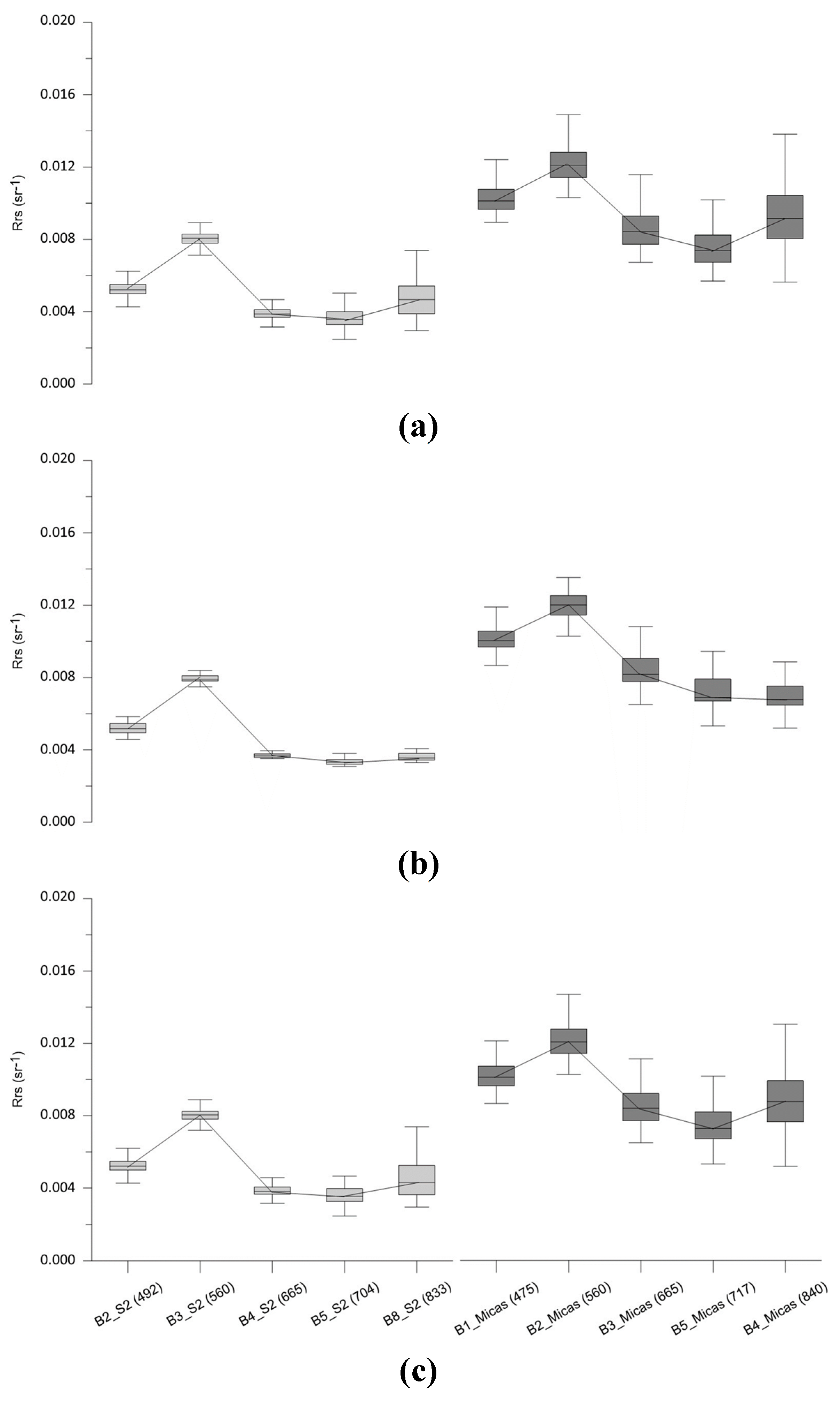
Another source of uncertainty regarding AC is the adjacency effect related to the distance to shore. This effect cause that the reflected light field from the neighboring land pixels, which are brighter, gets into the path from the target (water pixel) to the sensor through atmospheric scattering [64]. This also makes the reflectance value from the water pixels near the coast larger, and, hence, these datasets are prone to errors for the derivation of water quality parameters. This effect has been shown in the analysis made in our study comparing the Rrs reflectance of the outer and central pixels of the reservoir. Our results show how the Rrs reflectance of outer pixels have a higher value in the NIR band (B8 S2 MSI) than the central ones. This high NIR reflectance over inland and coastal waters due to adjacency effects has been already reported based on airborne and spaceborne data [8]. In the study of Warren et al. [60], it was also shown that iCOR performed poorly in coastal waters but much better in inland waters, due to the land/based methodologies applied to this processor. This result supports the use of iCOR when adjacency effects can be challenging, as in our case.

In spite of this, not only in our study but in some others using different AC processors [59,61] and methodologies [46], promising results were obtained in retrieving chl-a using red and NIR band combinations from Sentinel 2 MSI data. Further developments in the correction of these bands and the specific correction of the adjacency effects, which is only built-in in iCOR of all the publicly available AC processors, it is expected to improve the retrieval of chl-a in inland waters and reduce the associated uncertainties.

The propagation of these errors until the product output is leading to the uncertainties found in our product validation phase. The uncertainty associated with the final output of our Remote Sensing chain was evaluated for every model with different pairwise metrics describing bias and accuracy, as is discussed below.

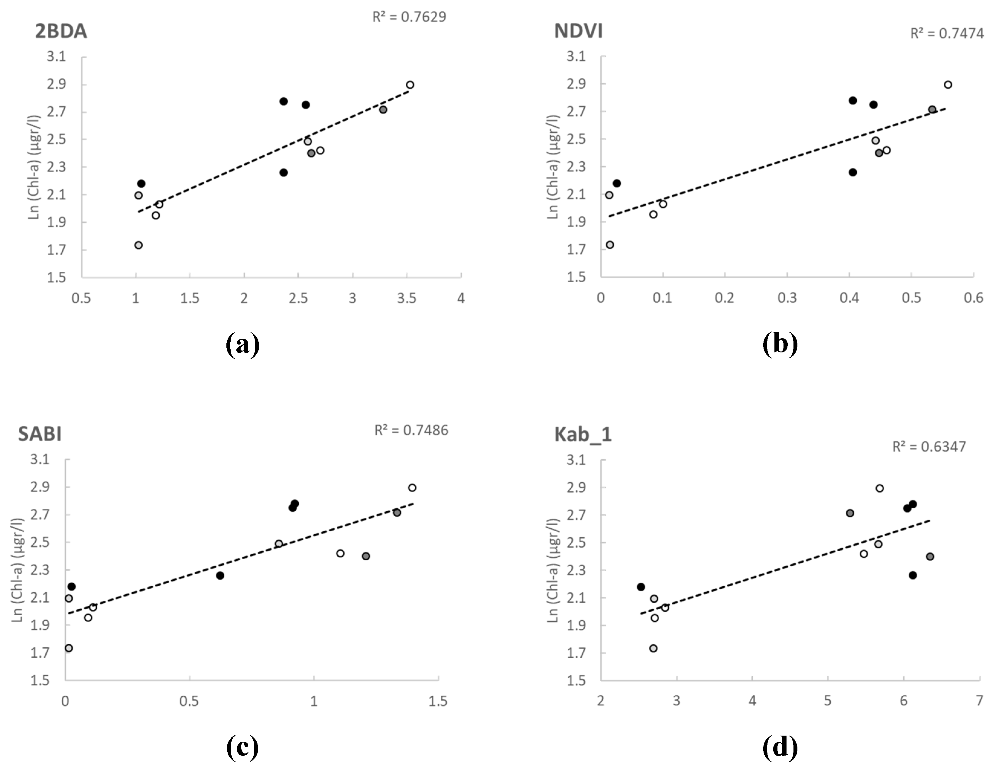
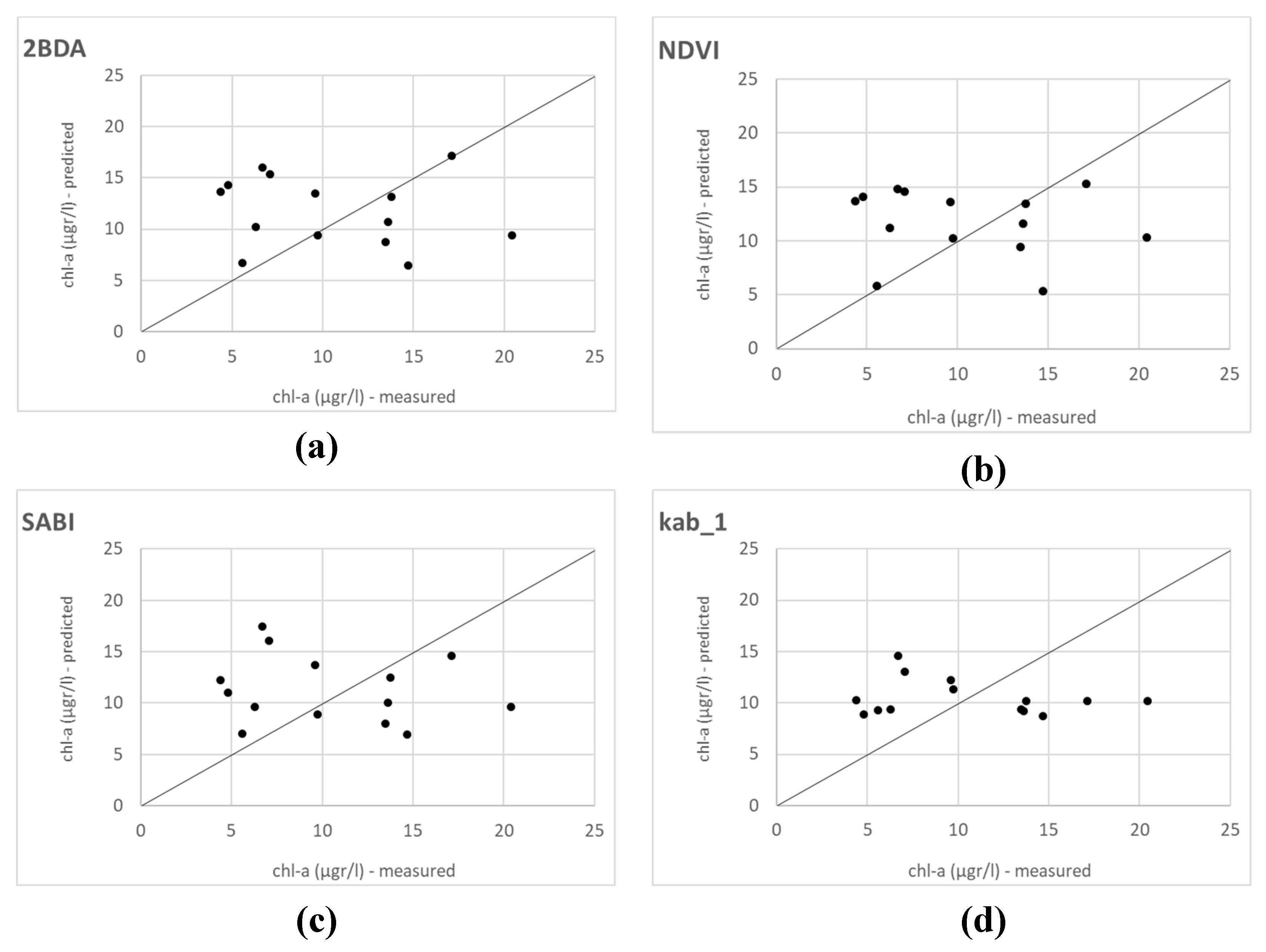
The development of algorithms for Landsat 8 OLI, with a spatial resolution of 30 m., is hampered by the small size of the reservoir, that makes the adjacency effects an important issue in this case [14]. Moreover, the need to move the match-up points in the reservoir from the shoreline in order to avoid this effect as much as possible can introduce a source of error in the algorithm development. Nevertheless, almost all the algorithms and Spectral Band Combinations tested were positively and significatively correlated with in situ chl-a values. Both the calibration and validation showed that the most appropriate Spectral Band Combinations in Landsat 8 OLI for the retrieval of chl-a were those based on red and NIR bands, specifically in our study: 2BDA, NDVI and SABI. The SABI is an empirical algorithm developed in order to detect water floating biomass that has an NIR response similar to land vegetation, and also includes blue and green spectral bands [48].

Although the correlations in the calibration of the models were good, our validation results did not show a good match between the measured and the predicted values (Figure 5). Other studies did not obtain good results with OLI data when developing algorithms applying 2BDA [38,51,58]. Watanabe et al. [38] found no relationship with simulated Rrs spectra for OLI/Landsat-8 based on field data in the eutrophic Barra Bonita Reservoir (Brazil), a bigger and deeper waterbody. In this work, also made in a higher chl-a concentration circumstance (mean values ranging from 120.4 to 428.7 µgr/L), the authors suggest that the 2BDA index, as proposed for clear waters, could not explain the chl-a distribution in their reservoir. The best results were obtained in this case with the SLOPE model developed by Mishra and Mishra [65], which uses red and green bands. Similarly, Boucher et al. [51] did not find a suitable model using the 2BDA algorithm with Landsat 8 images Level 1 corrected atmospherically with the dark object subtraction (DOS) method. In this study, made on a regional scale, including different lakes in New Hampshire and Maine (US), the best performing models where Kab1, Kab2 and KIVU, all based in blue and green bands. None of them used the L8SR product for the calibration of the models, which is also a methodological difference. This product has been evaluated for aquatic applications by Bernardo et al. [37]. L8SR was considered by the authors to provide suitable Rrs values for all OLI bands despite achieving the poorest results in Band 5 (NIR). However, our model calibration results with red and NIR bands show that this level 2 product made available by the USGS could be applied successfully for chl-a retrieval even in small waterbodies and should be further investigated with different trophic situations. Not only Red-NIR combinations were found correlated with in situ data in our study, but also algorithms using blue and green bands, as SABI, with very similar values in the validation of statistical metrics, but worst results in the validation graphical output. The worst results were obtained with all algorithms and indices using Band 1 (coastal-aerosol) (Kab2, B3B1 and GB1; cf. Table 3, Table 5 and Figure 4 and Figure 5). Our results confirm that green and blue band combinations are not the most suitable for retrieving chl-a in complex waters but also that the performance improves when Band 2 is used. This shows the difficulty of performing an accurate atmospheric correction for this ultra-blue band for inland aquatic applications. Wang et al. [66] also found big errors when computing band ratios with Band 1 data atmospherically corrected with different AC algorithms in their assessment of Landsat-8 OLI atmospheric correction algorithms for inland waters, even though they did not assess the L8SR product. The authors reported the same situation for the band ratios formed by the NIR band with all AC algorithms assessed.

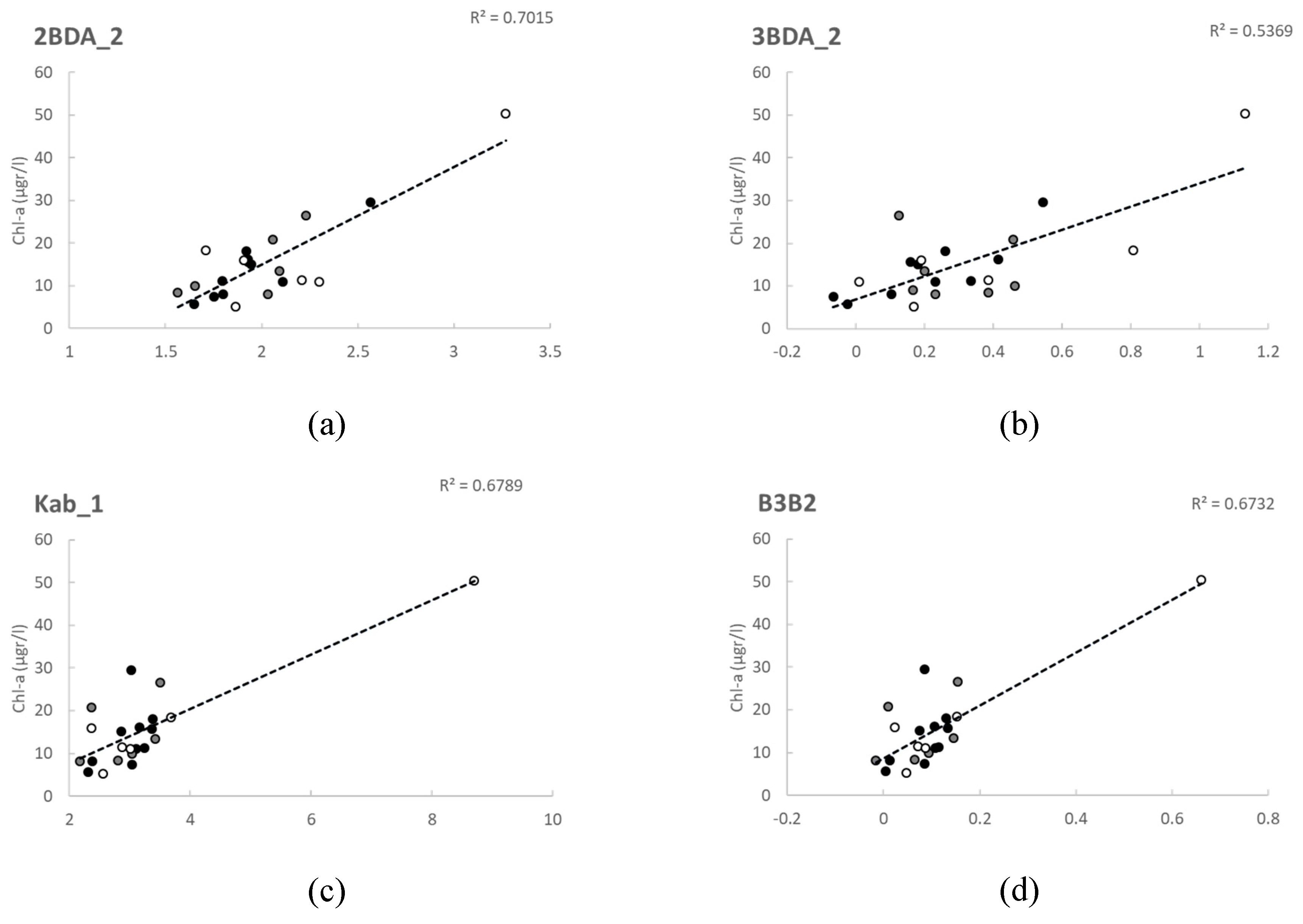
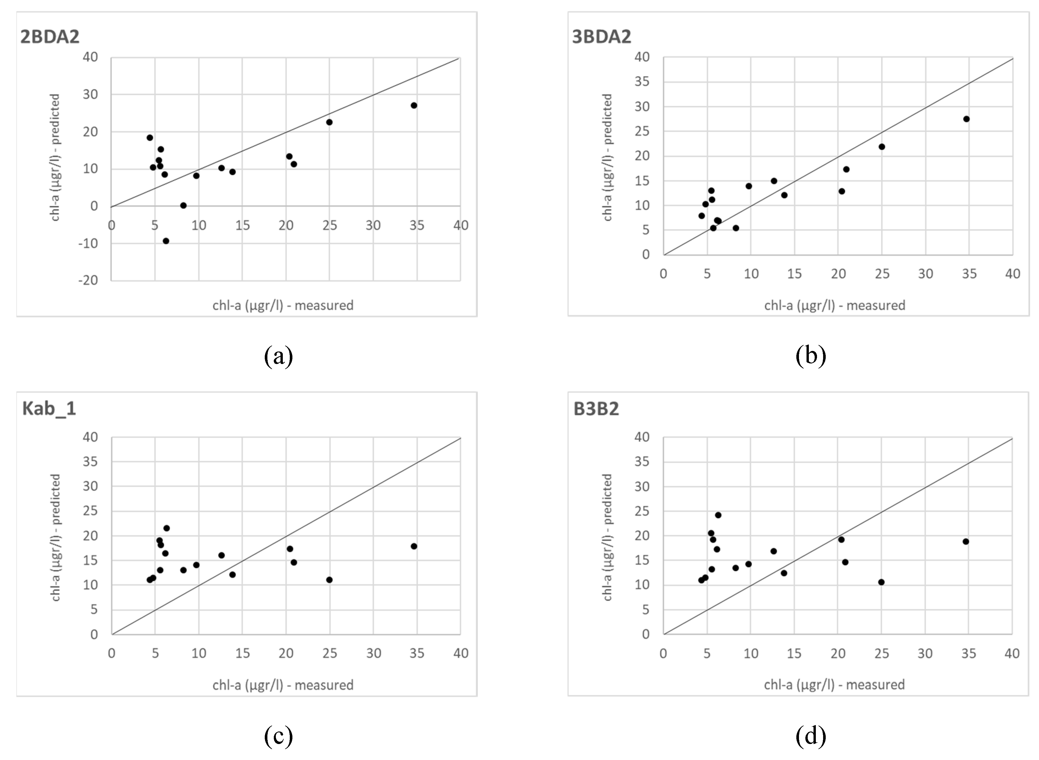
Sentinel 2 data have been extensively tested for chl-a retrieval since its launching in 2015 and 2017, both applying empirical and analytical modelling approaches [14,46,54,59,61,67]. Our results agree with the studies applying empirical modelling approaches [46,59,61], which evaluated the performance of the 3BDA model with good results, even though all of them used what we called here the 3BDA_1 version (with B6 as λ₃). Moreover, in agreement with our study are the results obtained by Xu et al. (2018), who also found good relationships with 3BDA, 2BDA and NDCI, although they used a different formulation of the 2BDA algorithm (B5/B4).

To the best of our knowledge, there is only one other study showing the performance of the commercial sensor Rededge Micasense for chl-a retrieval in waterbodies [68], but, in this case, the authors do not use Spectral band Combinations based in known spectral features of the chl-a but fit single and multiple variable linear approaches concluding that the best models in their case where those using green and red bands. We can nevertheless consider the results of our study as the first to test the algorithms developed, be proven effective for satellite remote sensing, adapted to Rededge Micasense sensor, and be tested in different trophic conditions. Again, the lack of field radiometry (as also happens in the study of Arango and Nairn [68]) entails a higher level of uncertainty in the final product. A radiometric calibration made by Cao et al. [69] for Rededge Micasense, showed in laboratory experiments a good relationship between ASD reflectance and Micasense with R² all above 0.96 for all bands. In field experiments, the comparison with the Pix4D processed image showed lower accuracy (overestimation) in the rededege and NIR regions, but a consistency in the spectral signature shape which reduced the uncertainty when using normalized indices.

When analyzing separately each flight data, the most suitable algorithms were again different combinations of red and NIR bands, including a modification of the 3BDA which excludes the last part of the equation. In our case, using the first computation involving λ₁ and λ₂, without removing the effect of the backscattering of the medium with the use of λ₃, gave the best results with this sensor in low chl-a conditions. The optimal position of λ₃ in 2BDA and 3BDA algorithms were established in practice by Dall’Olmo and Gitelson [70] in 720–740 nm in turbid productive waters. The NIR band of the Rededege Micasense is centered in 840 nm, hence too far from the optimal range, and proved not useful in our study in low chl-a values. As expected by the formulation of the algorithm, when applied in turbid conditions with high chl-a during the second UAV flight, this modification did not perform well (R² = 0.4; Pearson r = 0.6) as the effect of the backscattering of a medium with a high load of suspended particles should be removed with the λ₃ spectral region. Therefore, in this case 2BDA and SABI were the best performing algorithm in the presence of a bloom and high chl-a concentration. Again, the NIR spectral band in Rededge Micasense, used in this version of the 2BDA model in coherence with the formulation initially used for 3BDA, is far away from the optimal 720–740 nm range established by Dall’Olmo and Gitelson [70] to be used turbid productive waters, but performed better than the version of this algorithm made with the rededge band (2BDA_2). This band is centered in 717 nm, nearer of the optimum range, but the authors describe the aim of this band λ₃ as to be in a spectral region where the absorption by pigments, tripton and CDOM is negligible, which is something that happens at λ > 740 [21] so the use of longer wavelengths (840 nm in our case) might be feasible. Moreover, as chl-a increases, the λ₃ spectral region of maximal sensitivity to chl-a shifts toward longer wavelengths, and the precise optimal position of λ₁ and λ₃ will depend on the relative importance of the interferences and on the trophic status of the waterbody [70].

When analyzing the data of both flights in a combined dataset, NIR and red bands got lower correlations than the combination of blue-green and red-green. These last combinations were the best to discriminate the differences between very different chl-a concentrations, being this also reported by Arango and Nairn [68] with the same sensor. They also developed the models with data of two opposite trophic states and mean chl-a concentrations (oligotrophic: 8.52 µgr/L and eutrophic: 352.60 µgr/L) finding the green and red bands as the most significant.

This finding was used to develop a preliminary ensemble model for the retrieval of chl-a with UAV-Rededege data. In the ensemble model the pixels of the images were first classified in two chl-a classes, and subsequently a second model calibrated for that chl-a class was applied to every pixel to obtain a more accurate result. This model is still to be validated and further research will be done in next years to obtain data in intermediate and higher trophic states chl-a classes.

Our results show that the most suitable algorithms for the three combinations of platforms and sensors were those using NIR and red bands, and that 3BDA and its special case 2BDA were the most successful in retrieving chl-a with all the sensors tested. Beck et al. [71] obtained similar results when identifying the most “portable” algorithms for the quantification of chl-a. In their study, images from an airborne hyperspectral sensor (CASI) taken simultaneously with dense in situ water quality measurements, and synthetic multispectral datasets, yielded to the conclusion that the NDCI, 2BDA, and 3BDA chl-a algorithms were the most portable, being successful between hyperspectral imagers, WorldView-2 and -3, and Sentinel-2, MERIS-like imagers and, to a lesser degree, MODIS-like imagers.

The overall performance of our approach shows that the use of satellite data as baseline monitoring for eutrophication can be feasible bycombining different sensors, even in very small waterbodies. In this study, we found coherent results when applying the algorithms developed in low to medium chl-a values (1–20 µgr/L) but these failed in retrieving higher concentrations, which could be caused by the “packaging effect” (e.g., [38,72]) but also highlights the need for a further development of new algorithms calibrated with higher chl-a data. As it has been stressed in a number of studies, remote sensing reflectance data in waters with a high level of optical complexity are affected by the concentration of different optically active constituents and, as such, a single algorithm is unlikely to perform adequately in all situations [46,73]. This issue can be solved by using different algorithms in different conditions, which in our case should be algorithms in high chl-a concentration status, to be used alternatively depending on the limits of applicability stated for each model [7,74]. The choice of the appropriate algorithm for each case needs the availability of “a priori data” that could be obtained through the use of autonomous buoys placed in the most representative point of the lake, with real time data acquisition, ingested by the system to apply the suitable algorithm in each case.

The satellite part of our approach has been designed with freely available data, both of global coverage (satellite imagery freely distributed by ESA and NASA) and in situ point measurements (Regional scale. GAIA Portal [28]). If a compromise between the different agencies responsible for water sampling and analysis could be reached, so that the sampling points were equally representative and valid for use in the calibration and validation (cal/val) of RS products in space and time, and made available as FAIR data, the monitoring of these systems would be enhanced by the spatial component offered by RS through cal/val exercises on a global scale. In this regard, the autonomous buoy networks usually deployed by research institutions, where data are collected at high frequency and made freely available through grassroot networks of global coverage like the Global Lake Observatory Network (GLEON), are of particular interest. These buoys are usually located in central areas of water bodies, i.e., in free-water pixels, perfectly valid for its use as calibration and validation match-up points for RS products.

5. Conclusions

The first objective of this work was to evaluate the combined performance of the chl-a retrieval of three different sensors and remote sensing platforms as a multi-scale approach to be included in the standard monitoring of eutrophication processes in small-sized water bodies, in an area of high cloud cover, such as Galicia (NW Iberian Peninsula), by developing empirical models for the retrieval of chl-a concentration.

Our results show that the best performing models for all sensors and platforms were those using NIR and red bands and that the three platforms can be used in combination to maximize the temporal and spatial resolution offered by any of them independently. The best performing models were first the 3BDA algorithm for Sentinel MSI data and, as a second option in the absence of Sentinel 2 MSI data, the NDVI for Landsat 8 OLI, all of which were validated in a chl-a range of 1–40 µgr/L. Both the improvement in atmospheric corrections above water, especially the accounting for adjacency effects in the AC processors, should be prioritized for the future improvement in the development of this kind of tool for small- and medium-sized water bodies.

The multispectral commercial sensor Rededge Micasense gave the best results in low chl-a values (below 3 µgr/L) with a modified version of the 3BDA algorithm, while, in a high chl-a concentration (85–100 µgr/L), the 2BDA and SABI models were the more successful. However, in the range 1–100 µgr/L, the combinations of blue and green and red and green bands were the most effective in discriminating chl-a values with this sensor. Three of the developed algorithms were combined in a preliminary ensemble model. Further research will be done to validate these models with different ranges of chl-a data to apply them to intermediate and higher chl-a classes.

The developed workflow, in its initial design, can be easily included in the current monitoring scheme of the regional authorities, as the algorithms to be applied to satellite images were calibrated and validated with the data provided by them on a regular basis. With little effort, consisting in the change in the localization of some sampling points from the current location to another more centered in the waterbody and a sampling scheme coincident with satellite overpass (prioritizing Sentinel 2 overpass date and time), the accuracy of these empirical models is expected to improve, reducing the uncertainty related to spatiotemporal collocation and adjacency effects, thus improving their predicting ability. This highlights the value of freely available data sources for capacity building and developing of effective monitoring tools that could maximize the safety of our aquatic resources.

References

1. Ibisch, R.; Austnes, K.; Borchardt, D.; Boteler, B.; Leujak, W.; Lukat, E.; Rouillard, J.; Schmedje, U.; Lyche Solheim, A. European Assessment of Eutrophication Abatement Measures across Land-Based Sources Inland, Coastal and Marine Waters; European Environment Agency: Copenhagen, Denmark, 2016; pp. 7–9. [Google Scholar]
2. Lemley, D.A.; Adams, J.B. Eutrophication. Earth Syst. Environ. Sci. 2019, 1, 86–90. [Google Scholar] [CrossRef]
3. European Environmental Agency. European Waters—Assessment of Status and Pressures; EEA Report No. 8/2012; European Environment Agency: Copenhagen, Denmark, 2012; Available online: http://www.eea.europa.eu/publications/european-waters-assessment-2012 (accessed on 12 December 2019).
4. The European Parliament the Council of the European Union WFD. Directive 2000/60/EC of the European Parliament of the Council of 23 October 2000 establishing a framework for Community action in the field of water policy. OJL 2000, 327, 1–73. [Google Scholar]
5. Clean Water Act. Federal Water Pollution Control Act [As Amended Through P.L. 107–303, 27 November 2002]; United Stated Environmental Protection Agency: Washington, DC, USA, 2002. Available online: https://www.epa.gov/sites/production/files/2017-08/documents/federal-water-pollution-control-act-508full.pdf (accessed on 2 December 2019).
6. Brezonik, P.; Menken, K.D.; Bauer, M. Landsat-based remote sensing of lake water quality characteristics, including chlorophyll and colored dissolved organic matter (CDOM). Lake Reserv. Manag. 2005, 21, 373–382. [Google Scholar] [CrossRef]
7. Kutser, T.; Metsamaa, L.; Strömbeck, N.; Vahtmäe, E. Monitoring cyanobacterial blooms by satellite remote sensing. Estuar. Coast. Shelf. Sci. 2006, 67, 303–312. [Google Scholar] [CrossRef]
8. Moses, W.J.; Gitelson, A.A.; Berdnikov, S.; Povazhnyy, V. Satellite estimation of chlorophyll—A concentration using the red and NIR bands of MERIS—The Azov Sea case study. IEEE Geosci. Remote Sens. Lett. 2009, 6, 845–849. [Google Scholar] [CrossRef]
9. Matthews, M.W. A current review of empirical procedures of remote sensing in inland and near-coastal transitional waters. Int. J. Remote Sens. 2011, 32, 6855–6899. [Google Scholar] [CrossRef]
10. Matthews, M.W. Eutrophication and cyanobacterial blooms in South African inland waters: 10 years of MERIS observations. Remote Sens. Environ. 2014, 155, 161–177. [Google Scholar] [CrossRef]
11. Shi, K.; Zhang, Y.; Liu, X.; Wang, M.; Qin, B. Remote sensing of diffuse attenuation coefficient of photosynthetically active radiation in Lake Taihu using MERIS data. Remote Sens. Environ. 2014, 140, 365–377. [Google Scholar] [CrossRef]
12. Giardino, C.; Bresciani, M.; Stroppiana, D.; Oggioni, A.; Morabito, G. Optical remote sensing of lakes: An overview on Lake Maggiore. J. Limnol. 2014, 73, 201–214. [Google Scholar] [CrossRef] [Green Version]
13. Dörnhöfer, K.; Oppelt, N. Remote sensing for lake research and monitoring—Recent advances. Ecol. Indic. 2016, 64, 105–122. [Google Scholar] [CrossRef]
14. Anster, A.; Alikas, K. Retrieval of Chlorophyll a from Sentinel-2 MSI Data for the European Union Water Framework Directive Reporting Purposes. Remote Sens. 2019, 11, 64. [Google Scholar] [CrossRef] [Green Version]
15. Gitelson, A. The peak near 700 nm on radiance spectra of algae and water: Relationships of its magnitude and position with chlorophyll concentration. Int. J. Remote Sens. 1992, 13, 3367–3373. [Google Scholar] [CrossRef]
16. Kirk, J.T. Light and Photosyntesis in Aquatic Ecosystems, 2nd ed.; Cambridge University Press: Cambridge, UK, 1994; p. 509. [Google Scholar]
17. Mobley, C.D. Light and Water: Radiative Transfer in Natural Waters; Academic Press: Cambridge, MA, USA, 1994; p. 608. [Google Scholar]
18. Morel, A.; Prieur, L. Analysis of variations in ocean color. Limnol. Oceanogr. 1977, 22, 709–722. [Google Scholar] [CrossRef]
19. Witter, D.L.; Ortiz, J.D.; Palm, S.; Heath, R.T.; Budd, J.W. Assessing the application of SeaWiFS ocean color algorithms to Lake Erie. J. Great Lakes Res. 2009, 35, 361–370. [Google Scholar] [CrossRef]
20. Horion, S.; Bergamino, N.; Stenuite, S.; Descy, J.P.; Plisnier, P.D.; Loiselle, S.A.; Cornet, Y. Optimized extraction of daily bio-optical time series derived from MODIS/aqua imagery for Lake Tanganyika, Africa. Remote Sens. Environ. 2010, 114, 781–791. [Google Scholar] [CrossRef]
21. D’all Olmo, G.; Gitelson, A.; Rundquist, D.C. Towards a unified approach for remote estimation of chlorophyll-a in both terrestrial vegetation and turbid productive waters. Geophys. Res. Lett. 2003, 30, 1–4. [Google Scholar] [CrossRef] [Green Version]
22. Gitelson, A.A.; Dall’Olmo, G.; Moses, W.; Rundquist, D.C.; Barrow, T.; Fisher, T.R.; Gurlin, D.; Holz, J. A simple semi-analytical model for remote estimation of chlorophyll-a in turbid waters: Validation. Remote Sens. Environ. 2008, 112, 3582–3593. [Google Scholar] [CrossRef]
23. Gitelson, A.A.; Gurlin, D.; Moses, W.; Barrow, T. A bio-optical algorithm for the remote estimation of the chlorophyll-a concentration in case 2 waters. Environ. Res. Lett. 2009, 4, 1–5. [Google Scholar] [CrossRef]
24. Domínguez, J.A.; Alonso, C.; Alonso, A. Remote sensing as a tool for monitoring water quality parameters for Mediterranean Lakes of European Union water framework directive (WFD) and as a system of surveillance of cyanobacterial harmful algae blooms (SCyanoHABs). Environ. Monit. Assess. 2011, 181, 317–334. [Google Scholar] [CrossRef]
25. Li., J.; Roy, D.P. A Global Analysis of Sentinel-2A, Sentinel-2B and Landsat-8 Data Revisit Intervals and Implications for Terrestrial Monitoring. Remote Sens. 2017, 9, 902. [Google Scholar] [CrossRef] [Green Version]
26. Pahlevan, N.; Chittimalli, S.K.; Balasubramanian, S.V.; Vellucci, V. Sentinel-2/Landsat-8 product consistency and implications for monitoring aquatic systems. Remote Sens. Environ. 2019, 220, 19–29. [Google Scholar] [CrossRef]
27. Meteogalicia. Available online: https://www.meteogalicia.gal/ (accessed on 2 February 2018).
28. GAIA. Available online: https://gaia.xunta.es/plataforma/temas/agua/roaga/seguimiento-embalses/consulta-mediciones (accessed on 5 January 2020).
29. Welschmeyer, N. Fluorometric analysis of chlorophyll a in the presence of chlorophyll b and pheopigments. Limnol. Oceanogr. 1994, 39, 1985–1992. [Google Scholar] [CrossRef]
30. Gordon, H.R.; McCunley, W.R. Estimation of the depth of sunlight penetration in the sea for remote- sensing. Appl. Opt. 1975, 4, 413–416. [Google Scholar] [CrossRef] [PubMed]
31. Jeffrey, S.W.; Humphrey, G.F. New spectrophotometric equations for determining chlorophylls a, b, c1 and c2 in higher plants, algae and natural phytoplancton. Biochem. Physiol. Pflanzen. 1975, 167, 191–194. [Google Scholar] [CrossRef]
32. American Public Health Association, American Water Works Association and Water Environmental Federation. APHA Standard Methods for the Examination of Water and Wastewater, 20th ed.; American Public Health Association, American Water Works Association and Water Environmental Federation: Washington, DC, USA, 1998; p. 874.
33. Quesada, A. Ficobilinas o Ficobiliproteínas. In Estudio de las Aguas Continentales Mediante Teledetección; Domínguez, J.A., Marcos, C., Chao, Y., Delgado, G., Rodríguez, D., Eds.; Universidad Nacional de Educación a Distancia: Madrid, Spain, 2011; pp. 82–85. [Google Scholar]
34. De Keukelaere, L.; Sterckx, S.; Adriaensen, S.; Knaeps, E.; Reusen, I.; Giardino, C.; Bresciani, M.; Hunter, P.; Neil, C.; Van der Zande, D.; et al. Atmospheric correction of Landsat-8/OLI and Sentinel-2/MSI data using iCOR algorithm: Validation for coastal and inland Waters. Eur. J. Remote Sens. 2018, 51, 525–542. [Google Scholar] [CrossRef] [Green Version]
35. U.S. Geological Survey. LANDSAT 8 Surface Reflectance Code (Lasrc) Product Guide. V 2.0; U.S. Geological Survey: Reston, VA, USA, 2019; p. 39.
36. Pahlevan, N.; Schott, J.R.; Franz, B.A.; Zibordi, G.; Markham, B.; Bailey, S.; Schaaf, C.B.; Ondrusek, M.; Greb, S.; Strait, C.M. Landsat 8 remote sensing reflectance (Rrs) products: Evaluations, intercomparisons, and enhancements. Remote Sens. Environ. 2017, 190, 289–301. [Google Scholar] [CrossRef]
37. Bernardo, N.; Watanabe, F.; Rodrigues, T.; Alcantara, E. Atmospheric correction issues for retrieving total suspended matter concentrations in inland waters using OLI/Landsat-8 image. Adv. Space Res. 2017, 59, 2335–2348. [Google Scholar] [CrossRef] [Green Version]
38. Watanabe, F.; Alcantara, E.; Rodrigues, T.; Rotta, L.; Bernardo, N.; Imai, N. Remote sensing of the chlorophyll-a based on OLI/Landsat-8 and MSI/Sentinel-2A (Barra Bonita reservoir, Brazil). Ann. Braz. Acad. Sci. 2017, 90, 1–14. [Google Scholar] [CrossRef] [Green Version]
39. R Core Team. R: A Language and Environment for Statistical Computing; R Foundation for Statistical Computing: Vienna, Austria, 2018; Available online: https://www.R-project.org/ (accessed on 5 May 2020).
40. Bivand, R.; Keitt, T.; Rowlingson, B. rgdal: Bindings for the ‘Geospatial’ Data Abstraction Library. R Package Version 1.4-4. 2019. Available online: https://CRAN.R-project.org/package=rgdal (accessed on 5 May 2020).
41. Hijmans, R.J. raster: Geographic Data Analysis and Modeling. R Package Version 2.9-5. 2019. Available online: https://CRAN.R-project.org/package=raster (accessed on 5 May 2020).
42. Wickham, H.; François, R.; Henry, L.; Müller, K. dplyr: A Grammar of Data Manipulation. R Package. Version 0.8.1. 2019. Available online: https://CRAN.R-project.org/package=dplyr (accessed on 5 May 2020).
43. Matt Dowle and Arun Srinivasan (2019). data.table: Extension of ‘data.frame’. R Package Version 1.12.2. 2019. Available online: https://CRAN.R-project.org/package=data.table (accessed on 5 May 2020).
44. Gitelson, A.A.; Gritz, Y.; Merzlyak, M.N. Relationship between leaf chlorophyll content and spectral reflectance and algorithms for non-destructive chlorophyll assessment in higher plant leaves. J. Plant Physiol. 2003, 160, 271–282. [Google Scholar] [CrossRef]
45. Dall’Olmo, G.; Gitelson, A.A. Effect of bio-optical parameter variability on the remote estimation of chlorophyll-a concentration in turbid productive waters: Experimental results. Appl. Opt. 2005, 44, 412–422. [Google Scholar] [CrossRef] [Green Version]
46. Xu, M.; Hongxing, L.; Beck, R.; Lekki, J.; Yang, B.; Shu, S.; Kang, E.L.; Anderson, R.; Johansen, R.; Emery, E.; et al. A spectral space partition guided ensemble method for retrieving chlorophyll-a concentration in inland waters from Sentinel-2A satellite imagery. J. Great Lakes Res. 2019, 45, 454–465. [Google Scholar] [CrossRef]
47. Kabbara, N.; Benkhelil, J.; Awad, M.; Barale, V. Monitoring water quality in the coastal area of Tripoli (Lebanon) using High-resolution satellite data. ISPRS J. Photogramm. Remote Sens. 2008, 63, 488–495. [Google Scholar] [CrossRef]
48. Alawadi, F. Detection of surface algal blooms using the newly developed algorithm surface algal bloom index (SABI). Proc. Int. Soc. Opt. Eng. 2010, 7825, 1–14. [Google Scholar] [CrossRef] [Green Version]
49. Brivio, P.A.; Giardino, C.; Zilioli, E. Determination of chlorophyll concentration changes in Lake Garda using an image-based radiative transfer code for Landsat TM images. Int. J. Remote Sens. 2001, 22, 487–502. [Google Scholar] [CrossRef]
50. Mishra, S.; Mishra, D.R. Normalized difference chlorophyll index: A novel model for remote estimation of chlorophyll-a concentration in turbid productive waters. Remote Sens. Environ. 2012, 117, 394–406. [Google Scholar] [CrossRef]
51. Boucher, J.; Weathers, K.C.; Norouzi, H.; Steele, B. Assessing the effectiveness of Landsat 8 chlorophyll-a retrieval algorithms for regional freshwater monitoring. Ecol. Appl. 2018, 28, 1044–1054. [Google Scholar] [CrossRef] [Green Version]
52. Walsby, A.E.; Hayes, P.K.; Boje, R.; Stal, L.J. The selective advantage of buoyancy provided by gas vesicles for planktonic cyanobacteria in the Baltic Sea. New Phytol. 1997, 136, 407–417. [Google Scholar] [CrossRef]
53. Agha, R.; Cires, S.; Wörmer, L.; Domínguez, J.A.; Quesada, A. Multi-scale strategies for the monitoring of fresh- water cyanobacteria: Reducing the sources of uncertainty. Water Res. 2012, 46, 3043–3053. [Google Scholar] [CrossRef]
54. Bresciani, M.; Cazzaniga, I.; Austoni, M.; Sforzi, T.; Buzzi, F.; Morabito, G.; Giardino, C. Mapping phytoplankton blooms in deep subalpine lakes from Sentinel-2A and Landsat-8 M. Hydrobiologia 2018, 824, 197–214. [Google Scholar] [CrossRef] [Green Version]
55. Woodcock, C.E. Uncertainty in Remote Sensing. In Uncertainty in Remote Sensing and GIS; Foody, G.M., Atkinson, P.A., Eds.; John Wiley & Sons, Ltd.: Hoboken, NJ, USA, 2002; pp. 19–24. [Google Scholar] [CrossRef]
56. Schott, J.R. Remote Sensing: The Image Chain Approach; Oxford University Press: New York, NY, USA, 1997. [Google Scholar] [CrossRef]
57. Loew, A.; Bell, W.; Brocca, L.; Bulgin, C.E.; Burdanowitz, J.; Calbet, X.; Donner, R.V.; Ghent, D.; Gruber, A.; Kaminski, T.; et al. Validation practices for satellite-based Earth observation data across communities. Rev. Geophys. 2017, 55, 779–817. [Google Scholar] [CrossRef] [Green Version]
58. Yang, Z.; Anderson, Y. Estimating Chlorophyll-A Concentration in a Freshwater Lake Using Landsat 8 Imagery. J. Environ. Earth Sci. 2016, 6, 134–142. [Google Scholar]
59. Toming, K.; Kutser, T.; Laas, A.; Sepp, M.; Paavel, B.; Nõges, T. First experiences in mapping lake water quality parameters with sentinel-2 MSI imagery. Remote Sens. 2016, 8, 640. [Google Scholar] [CrossRef] [Green Version]
60. Warren, M.A.; Simis, S.G.H.; Martinez-Vicente, V.; Poser, K.; Bresciani, M.; Alikas, K.; Spyrakos, E.; Giardino, C.; Ansper, A. Assessment of atmospheric correction algorithms for the Sentinel-2A MultiSpectral Imager over coastal and inland waters. Remote Sens. Environ. 2019, 225, 267–289. [Google Scholar] [CrossRef]
61. Pereira-Sandoval, M.; Urrego, P.; Ruiz-Verdú, A.; Tenjo, C.; Delegido, J.; Soria-Perpinyà, X.; Vicente, E.; Soria, J.; Moreno, J. Calibration and validation of algorithms for the estimation of chlorophyll-a concentration and Secchi depth in inland waters with Sentinel-2. Limnetica 2019, 38, 471–487. [Google Scholar] [CrossRef]
62. Ilory, C.O.; Pahlevan, N.; Knudby, A. Analyzing Performances of Different Atmospheric Correction Techniques for Landsat 8: Application for Coastal Remote Sensing. Remote Sens. 2019, 11, 469. [Google Scholar] [CrossRef] [Green Version]
63. Doxani, G.; Vermote, E.; Roger, J.C.; Gascon, F.; Adriaensen, S.; Frantz, D.; Hagolle, O.; Hollstein, A.; Kirches, G.; Li, F.; et al. Atmospheric correction inter-comparison exercise. Remote Sens. 2018, 10, 352. [Google Scholar] [CrossRef] [Green Version]
64. Moses, W.; Sterckx, S.; Montes, M.J.; De Keukelaere, L.; Knaeps, E. Atmospheric Correction for Inland Waters. In Bio-Optical Modeling and Remote Sensing of Inland Waters; Mishra, D.R., Ogashawara, I., Gitelson, A.A., Eds.; Elsevier Inc.: Amsterdam, The Netherlands, 2017; pp. 69–100. [Google Scholar] [CrossRef]
65. Mishra, D.R.; Mishra, S. Plume and bloom: Effect of the Mississippi River diversion on the water quality of Lake Pontchartrain. Geocarto Int. 2010, 25, 555–568. [Google Scholar] [CrossRef]
66. Wang, D.; Ma, R.; Xue, K.; Loiselle, S.A. The Assessment of Landsat-8 OLI Atmospheric Correction Algorithms for Inland Waters. Remote Sens. 2019, 11, 169. [Google Scholar] [CrossRef] [Green Version]
67. Ha, N.T.T.; Thao, N.T.P.; Koike, K.; Nhuan, M.T. Selecting the Best Band Ratio to Estimate Chlorophyll-a Concentration in a Tropical Freshwater Lake Using Sentinel 2A Images from a Case Study of Lake Ba Be (Northern Vietnam). Int. J. Geo-Inf. 2017, 6, 290. [Google Scholar] [CrossRef]
68. Arango, J.G.; Nairn, R.W. Prediction of Optical and Non-Optical Water Quality Parameters in Oligotrophic and Eutrophic Aquatic Systems Using a Small Unmanned Aerial System. Drones 2020, 4, 1. [Google Scholar] [CrossRef] [Green Version]
69. Cao, S.; Danielson, B.; Clare, S.; Koenig, S.; Campos-Vargas, C.; Sánchez-Azofeifa, A. Radiometric calibration assessments for UAS-borne multispectral cameras: Laboratory and field protocols. J. Photogramm. Remote Sens. 2019, 149, 142–145. [Google Scholar] [CrossRef]
70. Dall’ Olmo, G.; Gitelson, A. Effect of Bio-Optical Parameter Variability and Concentration in Turbid Productive Waters: Remote Estimation of Chlorophyll-a Uncertainties in Reflectance Measurements on the Modeling Results. Appl. Opt. 2006, 45, 3577–3592. Available online: http://digitalcommons.unl.edu/natrespapers/259 (accessed on 18 June 2019).
71. Beck, R.; Zhan, S.; Liu, H.; Tong, S.; Yang, B.; Xu, M. Comparison of satellite reflectance algorithms for estimating chlorophyll-a in a temperate reservoir using coincident hyperspectral aircraft imagery and dense coincident surface observations. Remote Sens. Environ. 2016, 178, 15–30. [Google Scholar] [CrossRef] [Green Version]
72. Bricaud, A.; Babin, M.; Morel, A.; Claustre, H. Variability in the chlorophyll-specific absorption coefficients of natural phytoplankton: Analysis and parameterization. J. Geophys. Res. 1995, 100, 321–332. [Google Scholar] [CrossRef]
73. Tyler, A.; Hunter, P.D.; Spyrakos, E.; Groomb, E.; Constantinescu, A.M.; Kitchen, J. Developments in Earth observation for the assessment and monitoring of inland, transitional, coastal and shelf-sea waters. Sci. Total Environ. 2016, 572, 1307–1321. [Google Scholar] [CrossRef] [PubMed] [Green Version]
74. Stumpf, R.P.; Tyler, M.A. Satellite detection of bloom and pigment distributions in estuaries. Remote Sens. Environ. 1988, 24, 385–404. [Google Scholar] [CrossRef]
Figure 1. Localization of the study site in Europe (A), in the NW of the Iberian Peninsula (B) and aerial picture of the reservoir with in situ sampling points both from the periodic monitoring [28] and from the two Unmanned Aerial Vehicle (UAV) flights (same sampling points for 2017 and 2018) (C).
Remotesensing 12 01514 g001
Figure 2. Graphical representation of spatial resolution and bandwidths of the three multispectral sensors used. Notation: S (Sentinel 2, MSI), L (Landsat 8, OLI) and R (Rededge Micasense), followed by the band number in each sensor.
Remotesensing 12 01514 g002
Figure 3. Workflow for Image processing and data analysis.
Remotesensing 12 01514 g003
Figure 4. Best performing models (models using the SBC: (a) 2BDA; (b) NDVI; (c) SABI and (d) Kab_1) for retrieving chl-a from Landsat 8 OLI data. The code color of the points reflects the time difference between the in situ data and the satellite image acquisition data: white: 0 days; light grey: 1 day; dark grey: 2 days and black: 3 days.
Remotesensing 12 01514 g004
Figure 5. Validation scatter plots for the best performing models for retrieving chl-a using Landsat 8 OLI data. Models using the SBC: (a) 2BDA; (b) NDVI; (c) SABI and (d) Kab_1). Line 1:1 is also shown.
Remotesensing 12 01514 g005
Figure 6. Best performing models for retrieving chl-a from Sentinel 2 MSI data (models using the SBC: (a) 2BDA_2; (b) 3BDA_2; (c) Kab_1 and (d) B3B2). The color code of the points reflects the time difference between the in situ data and the satellite image acquisition data: white: 0 day; dark grey: 2 days and black: 3 days (there are no match-ups with 1 day difference).
Remotesensing 12 01514 g006
Figure 7. Validation scatter plots for the best performing models for retrieving chl-a from Sentinel 2 MSI data. Models using the SBC: (a) 2BDA_2; (b) 3BDA_2; (c) Kab_1 and (d) B3B2. Line 1:1 is also shown.
Remotesensing 12 01514 g007
Figure 8. Best performing models for retrieving chl-a from Rededge Micasense on board UAV. 3BDA_MOD in (a) a low-chl-a condition which corresponds to 2017 flight data, and (b) and (c) high chl-a condition, which corresponds with 2018 flight data. The results correspond to the calculations made with data included in a 0.5, 1.0 and 1.5-m. buffers, which are shown following this order from top to base.
Remotesensing 12 01514 g008
Figure 9. Best performing models for retrieving chl-a from Rededge Micasense on board UAV when the data of both flights are combined. Models applying Spectral Band Combinations (a) B3B1; (b) GB1 and (c) G/B are shown.
Remotesensing 12 01514 g009
Figure 10. Application of the B3B1 algorithm to the images corresponding to the 2017 flight (low-chl-a) (a) and 2018 flight (high chl-a) (b). Legend indicates µgr/L of chl-a.
Remotesensing 12 01514 g010
Figure 11. Box-whiskers plot comparing the spectral signature of Sentinel 2 MSI and Rededge Micasense sensors for the images acquired on 10/02/2018. Figure (a) shows the results for the outer pixels in the reservoir. Figure (b) shows the results for the central pixels in the reservoir, and Figure (c) shows the results for the entire reservoir.
Remotesensing 12 01514 g011
Figure 12. Graphical results of the combining monitoring approach for chl-a in September and October 2017 and 2018. Thematic chl-a (µg/l) maps for Landsat 8 OLI, Sentinel 2 (A- B) MSI and UAV Rededge Micasense flights. The date column shows the satellite overpass. The in situ column shows the results of the periodic monitoring in the reservoir in the nearest date available (BC and BP sampling points in Figure 1) in the same color code (bottom color bar).
Remotesensing 12 01514 g012