A Deep Learning Model for Automatic Plastic Mapping Using Unmanned Aerial Vehicle (UAV) Data


1
Faculty of Architecture, Civil Engineering and Geodesy, University of Banja Luka, 78000 Banja Luka, Bosnia and Herzegovina
2
Faculty of Technical Science, University of Novi Sad, 21000 Novi Sad, Serbia
3
GEOINCA, Universidad de León, 24404 Ponferrada, Spain
*
Author to whom correspondence should be addressed.
Remote Sens. 2020, 12(9), 1515; https://0-doi-org.brum.beds.ac.uk/10.3390/rs12091515
Submission received: 1 April 2020
/
Revised: 3 May 2020
/
Accepted: 7 May 2020
/
Published: 9 May 2020
Abstract
:Although plastic pollution is one of the most noteworthy environmental issues nowadays, there is still a knowledge gap in terms of monitoring the spatial distribution of plastics, which is needed to prevent its negative effects and to plan mitigation actions. Unmanned Aerial Vehicles (UAVs) can provide suitable data for mapping floating plastic, but most of the methods require visual interpretation and manual labeling. The main goals of this paper are to determine the suitability of deep learning algorithms for automatic floating plastic extraction from UAV orthophotos, testing the possibility of differentiating plastic types, and exploring the relationship between spatial resolution and detectable plastic size, in order to define a methodology for UAV surveys to map floating plastic. Two study areas and three datasets were used to train and validate the models. An end-to-end semantic segmentation algorithm based on U-Net architecture using the ResUNet50 provided the highest accuracy to map different plastic materials (F1-score: Oriented Polystyrene (OPS): 0.86; Nylon: 0.88; Polyethylene terephthalate (PET): 0.92; plastic (in general): 0.78), showing its ability to identify plastic types. The classification accuracy decreased with the decrease in spatial resolution, performing best on 4 mm resolution images for all kinds of plastic. The model provided reliable estimates of the area and volume of the plastics, which is crucial information for a cleaning campaign.
Keywords:
deep learning; mapping plastic; automatic detection; AI; remote sensing; UAV; segmentation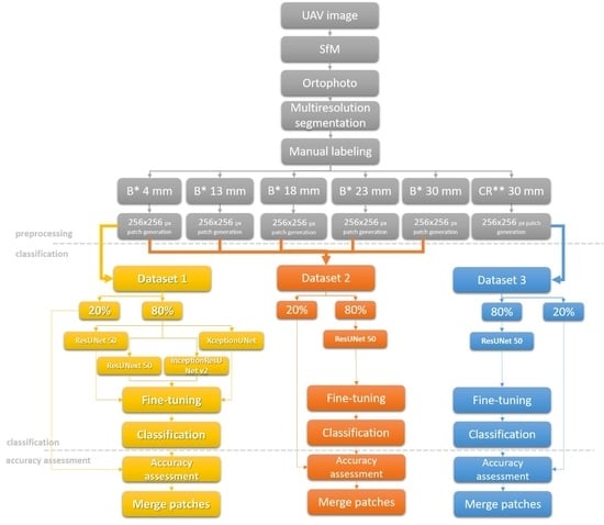
1. Introduction
Plastic pollution has become one of the most significant environmental issues of our age. Since the 1950s, when it was invented, as sanitary and cheap material, plastic took the place of paper and glass in food packaging, wood in furniture, and metal in car production. Global plastic production has increased annually, reaching almost 360 million tons in 2018 [1]. Only nine percent of the nine billion tons of plastic that has ever been produced has been recycled [2]. Subsequently, more than 8 million tons of plastic end up in the ocean each year [3]. Plastic is not biodegradable, and over time, macro plastic pieces degrade into smaller and smaller pieces called microplastic (less than five millimeters long [4]). Microplastic can be swallowed by a wide variety of marine organisms and then rise through the food chain, ending up on our dinner tables. Marine plastic litter is a global environmental problem with significant economic, ecological, public health, and aesthetic impacts. Effective measures to prevent negative effects of marine plastics require an understanding of its origin, pathways, and trends.
Land-based litter, transported by rivers to oceans, is estimated to be a major contributor to this problem [4,5]. The research presented by [6] estimates that just 10 river systems transport more than 90% of the global input. The global estimations of plastic debris entering oceans annually, although numerous, are typically based on local or regional scale surveys, and they vary from 250,000 tons [7] to 4.8–12.7 million tons of plastic [8]. Therefore, the amount of plastic in the global oceans remains poorly understood with a knowledge gap in terms of the temporal and spatial distribution of plastics, degradation, and beach processes. This information is vital for the development of activity plans for reducing land-based litter impact in oceans. Several efforts have been made to establish a standardized monitoring methodology, such as Oslo and Paris Conventions (OSPAR) [9], Commonwealth Scientific and Industrial Research Organization (CSIRO) [10], National Oceanic and Atmospheric Administration (NOAA) [11], and United Nations Environment Programme /Intergovernmental Oceanographic Commission (UNEP/IOC) [12]. Those methodologies are based on traditional beach monitoring by visual counting of plastic pieces along transects. Many guidelines on survey and monitoring of marine litter, such as OSPAR [9], NOAA [11], and UNEP/IOC [12] record the counts of all items larger than 2.5 cm × 2.5 cm, since this is the minimum disposal size permitted under the International Convention for the Prevention of Pollution from Ships (MARPOL) for ground shipping waste [13]. According to [12], each person is responsible for noticing or collecting all litter in the 2 m wide zone along a transect and, as a consequence, traditional beach surveys involve a large number of people. As an example, CSIRO engaged thousands of students, teachers, and employees in order to survey coastal debris in 175 sites in Australia, surveying 575 two-meter wide transects over a period of 18 months [10]. Visual surveys are, therefore, time and labor consuming, and usually only a sub-sample of the target study area is covered. In addition, the surveyors can be in unsafe situations due to heavy wind, slippery rocks, hazards such as rain and snow, or exposed to dangerous substances (such as chemical substances, medical waste, etc.). Plastic litter is mostly concentrated on banks, coastlines and in the upper layer of surface water bodies, mostly within the first 0.5 m [14]. Taking that into account, remote sensing technologies with a high spatial, temporal and spectral resolution have the potential to become reliable sources of information on floating plastics. Two examples of using these techniques have been provided by [15] and [16]. Jakovljevic et al. [15] developed an algorithm for the detection of floating plastic in freshwater, based on Artificial Neural Networks and high-resolution multispectral WorldView-2 images, reporting a Root Mean Square Error (RMSE) of 0.03 during the test phases. Aoyama [16] used high-resolution WordView-3 satellite images and the Spectral Angle Mapper algorithm for the extraction of marine debris in the Sea of Japan.
In recent years, Unmanned Aerial Vehicles (UAVs) have been recognized as an effective low-cost image-capturing platform, suitable for monitoring aquatic environments with high accuracy [17,18]. Customizable flight routes at low-level altitudes in combination with new algorithms for photogrammetric processing, such as the Structure from Motion (SfM) algorithm, provide a cost-effective acquisition of geospatial data with high spatial and temporal resolution, suitable for qualitative and quantitative analysis of natural and artificial structures of streams and floodplains. In addition to infrared and standard sensors, UAV can be equipped with multispectral cameras enabling its data to be combined with satellite imagery. Martin et al. [19] used high-resolution (<1 cm) UAV images and the Random Forest algorithm for the detection of plastic on the beaches, obtaining detection rates of 44%, 5%, and 3.7% for drinking containers, bottle caps, and plastic bags, respectively. Topouzelis et al. [20] compared the spectral response of Sentinel 2 and high-resolution UAV images over a large plastic floating target (100 m2). Geraeds et al. [21] used images obtained by UAV at different flight heights to manually label the riverbank and floating plastic. Moy et al. [22] created a hot spot map of debris on Hawaii Island beaches by visually interpreting orthorectified imagery mosaics with a ground sample distance of 2 cm. Although UAVs can provide appropriate spatial and temporal resolution to produce suitable data for mapping floating plastic, most of the methods developed so far are based on visual interpretation and manual labeling of plastic pieces, which is time-consuming and labor-intensive.
Recently, the deep Convolution Neural Network (CNN) has been widely used in image classification tasks such as automatic classification, object detection [17,18], and semantic segmentation [23,24,25]. With the rapid improvement of Graphics Processing Unit (GPU) computing and the increase of open training datasets, CNN models, such as AlexNet [26], VGGNet [27], ResNet [28], DenseNet [29], and Inception [30], used for image classification or for semantic segmentation in combination with Fully Convolutional Network (FCN), U-Net or DeepLab architecture, have achieved state-of-art accuracy in this topic. However, they completely discard the spatial information in the top layer, thus, producing a lack of accurate positioning and class boundary characterization.
Semantic segmentation aims to assign the set of predefined class labels to each pixel in the image. In early research, deep semantic segmentation used the patch-based CNN method [31,32], where images are first divided into patches and then fed into CNN networks. The network predicts the central pixel label based on the surrounding image patches. This process is repeated for each pixel, producing a high computational cost, especially in overlapping patches. To solve this problem Long et al. [33] proposed to use a Fully Convolutional Network (FCN). The FCN is an end-to-end model that maintains a two-dimensional structure of a feature map and uses contextual and location information to predict class labels, reducing the computational cost significantly. Semantic segmentation models based on FCN can be divided into four categories: encoder-decoder structure [23,24], dilated convolutions [34], and spatial pyramid pooling [35], which are described below.
The encoder-decoder structure is widely applied to semantic segmentation. Firstly, the encoder generates feature maps with high-level semantic but low resolution by using convolutions, pooling and an activation layer. Finally, the decoder upsamples the low-resolution encoder feature maps, retrieving the location information and obtaining fine-scaled segmentation results. SegNet [23] and U-Net [24] are typical architectures with encoder-decoder structures. On the one hand, SegNet [23] stores the index of each max pooling window in the encoder, which then stores the indices of the maximum pixel, so the decoders upsample the input using the indices coming from the encoder stage. On the other hand, U-Net [24] is a highly symmetric U-shaped architecture where the skip connection is used to directly link the output of each level from encoder to the corresponding level of the decoder. Therefore, comparing U-Net to SegNet, the first does not reuse indices but instead it transfers the entire feature map to the corresponding decoders and consonant them to the upsampled decoder feature maps. This process produces more accurate maps than using SegNet, but it consumes more memory [23]. Also, U-Net can produce a precise segmentation with very few training images [24]. Zhao et al. [36] used UAV RGB and multispectral images and U-Net architecture to extract rice lodging, obtaining the dice coefficients of 0.94 and 0.92, respectively. Xu et al. [37] used ResUNet for building extraction from Very High Resolution (VHR) multispectral satellite images reporting an F1 score of 0.98. In that case, the ResUNet adopted the U-Net as basic architecture but the U-Net learning units were replaced with residual learning units. Similarly, Yi et al. [38] used DeepResUNet and aerial VHR to map urban buildings, reaching high accuracies (F1 score: 0.93).
Chen et al. [35] introduced DeepLab architecture, which uses a parallel atrous convolution design instead of deconvolution for upsampling, performing similarly to other state-of-the-art models. Recent studies show that U-Net architecture outperforms DeepLab in cases with complex water environments [39,40]. Furthermore, U-Net architecture is preferred to DeepLab architecture because due to a higher number of hyperparameters the DeepLab architecture is more computationally intensive (processing time is increased by 58%) [39] and it needs more training steps to reach a performance comparable to U-Net [40].
The first step in addressing the ocean’s plastic problem is to do an estimation of the amount of plastic, where it is accumulating and its pathways. However, the differences in the protocols which attempt to monitor the temporal and spatial distribution of plastic pollution (OSPAR [9], CSIRO [10]), and the fact that the accuracy of the collected data varies depending on the observer’s skill, make the integration and comparison of the estimations challenging. The research presented in this paper aims to fulfill the need for an efficient and rapid estimation of floating plastic. The main goals of this paper are to: (1) examine the performance of different deep learning algorithms for mapping floating plastic using high-resolution UAV images, (2) to examine the relationship between the spatial resolution of the UAV imagery and the size of the detected plastic, (3) to test the possibility of mapping different plastic materials such as Oriented Polystyrene (OPS), Polyethylene terephthalate (PET), and Nylon, and (4) to define a methodology for UAV surveying to map floating plastic.
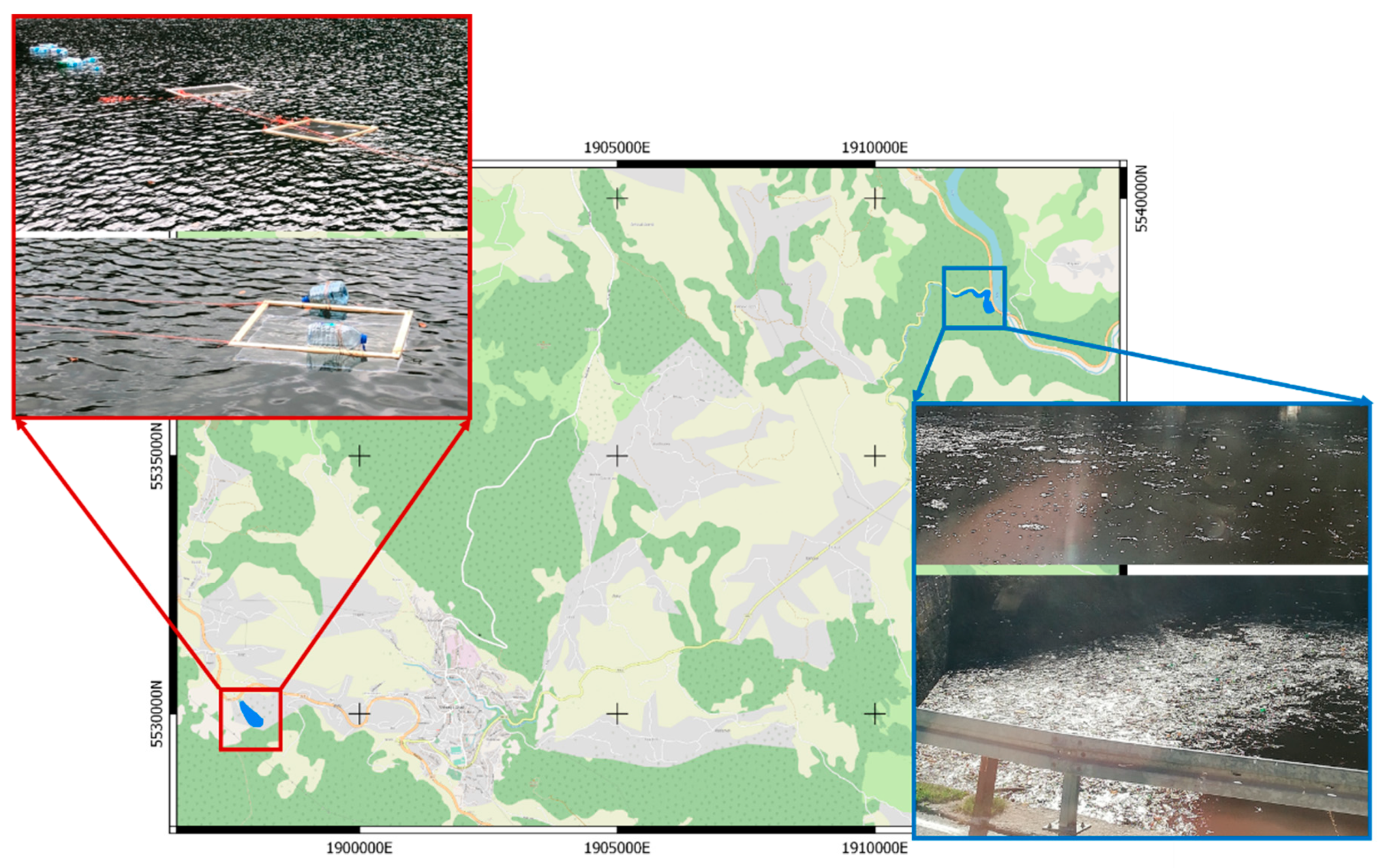
2. Study Area
Two study areas near Mrkonjić Grad (Bosnia and Herzegovina) were defined (Figure 1): (i) the artificial Lake Balkana, with clear water, and (ii) the confluence of the Crna Rijeka and the Vrbas Rivers.
3. Materials
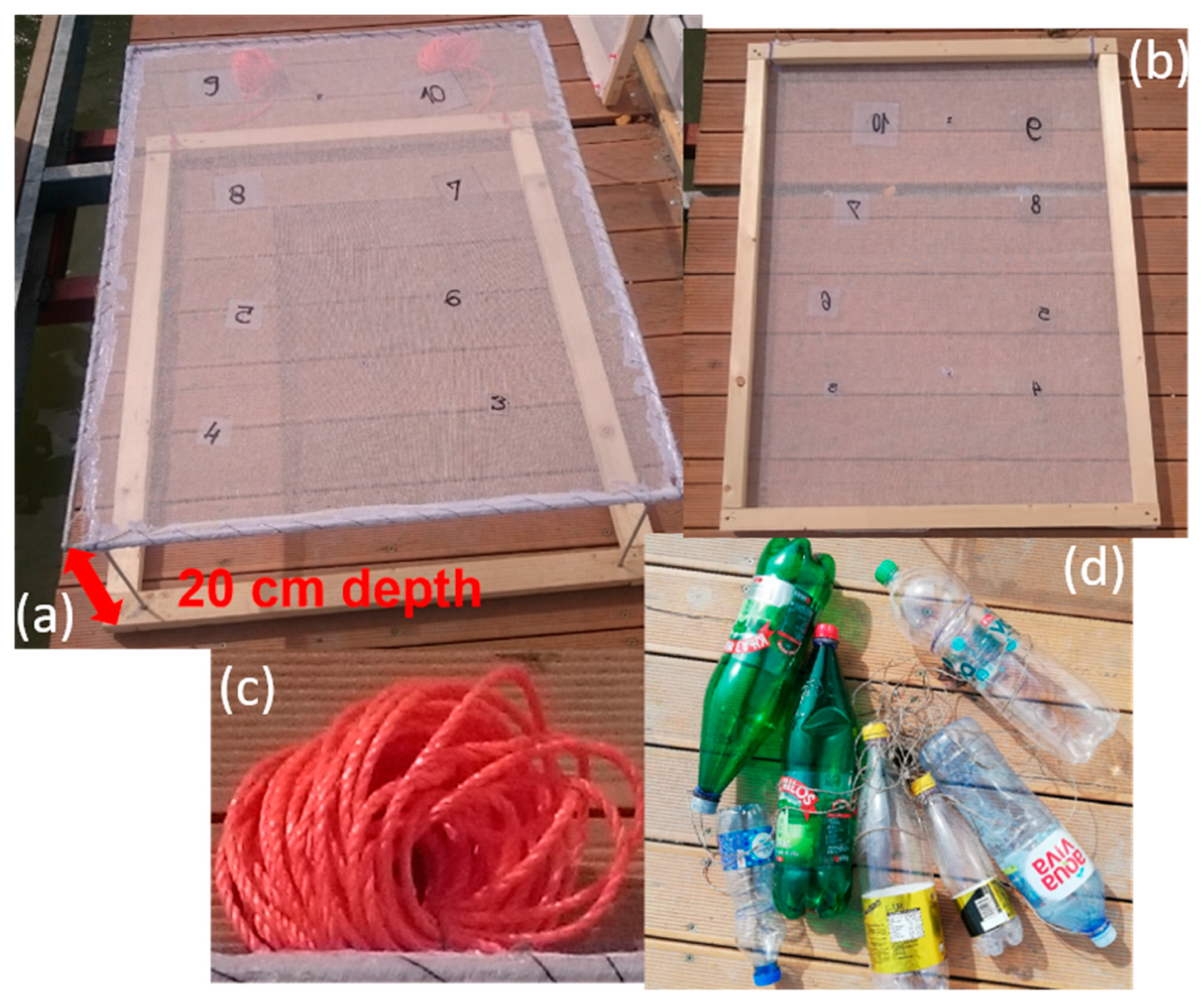
For the study area in the artificial Lake Balkana, targets were designed to examine the possibility of mapping plastics of different sizes using UAV imagery. The targets consisted of (i) a wooden frame (100 cm × 80 cm) with thin and transparent gauze and plastic squares, with side lengths from 1 to 10 cm (Figure 2b), (ii) a wooden frame (100 cm × 80 cm) with thin and transparent gauze and plastic squares, with sides from 11 to 16 cm long, (iii) a wooden frame (100 cm × 80 cm) attached to a metal frame located 20 cm below it, with thin and transparent gauze and plastic squares, with sides from 1 to 10 cm long (Figure 2a), and (iv) plastic bottles of different sizes and colors connected by ropes (Figure 2d). A rope with a diameter of 4 mm was used to keep the frames in the area of interest during the surveys (Figure 2c), while the wood made them floatable. The targets were released in the water in the deepest part of the lake, to exclude the reflection of the lake bottom. Besides, three different plastic materials were used: OPS (used for the plastic squares (Figure 2a,b), PET (plastic bottles Figure 2d)), and Nylon (rope Figure 2c).
For the second study area, upstream of the confluence of the Crna Rijeka and the Vrbas Rivers a net for collecting floating garbage was installed. Floating waste is the major source of litter in this area, due to the disposal of the garbage in illegal landfills and picnic sites along the river or directly in the river. The net collects about 10,000 m3 of material annually, from which 60% is wood, 35% plastic packaging, and 5% other [41]. The plastic packaging consists of 55% PET, while 45% consists of Polyethylene (PE), and Polypropylene (PP) [41]. The amount of litter depends mostly on the weather conditions. The largest quantity is captured during the rainy periods (spring and autumn) when water level increases and washes away the garbage from the river banks. In May 2019, due to heavy rains, the net broke and 10,000 tons of floating garbage ended up in the head pond of the hydroelectric power plant. In order to detect and map the plastic (the self-built targets and the plastic stopped by the net), 6 UAV surveys were conducted, using a DJI Mavic pro equipped with an RGB camera. Five surveys with different flight heights (12–90 m) took place over the Balkana Lake area, and one (at a 90 m flight height) over the Crna Rijeka River. The flight heights and spatial resolutions of the surveys are presented in Table 1.
4. Methods
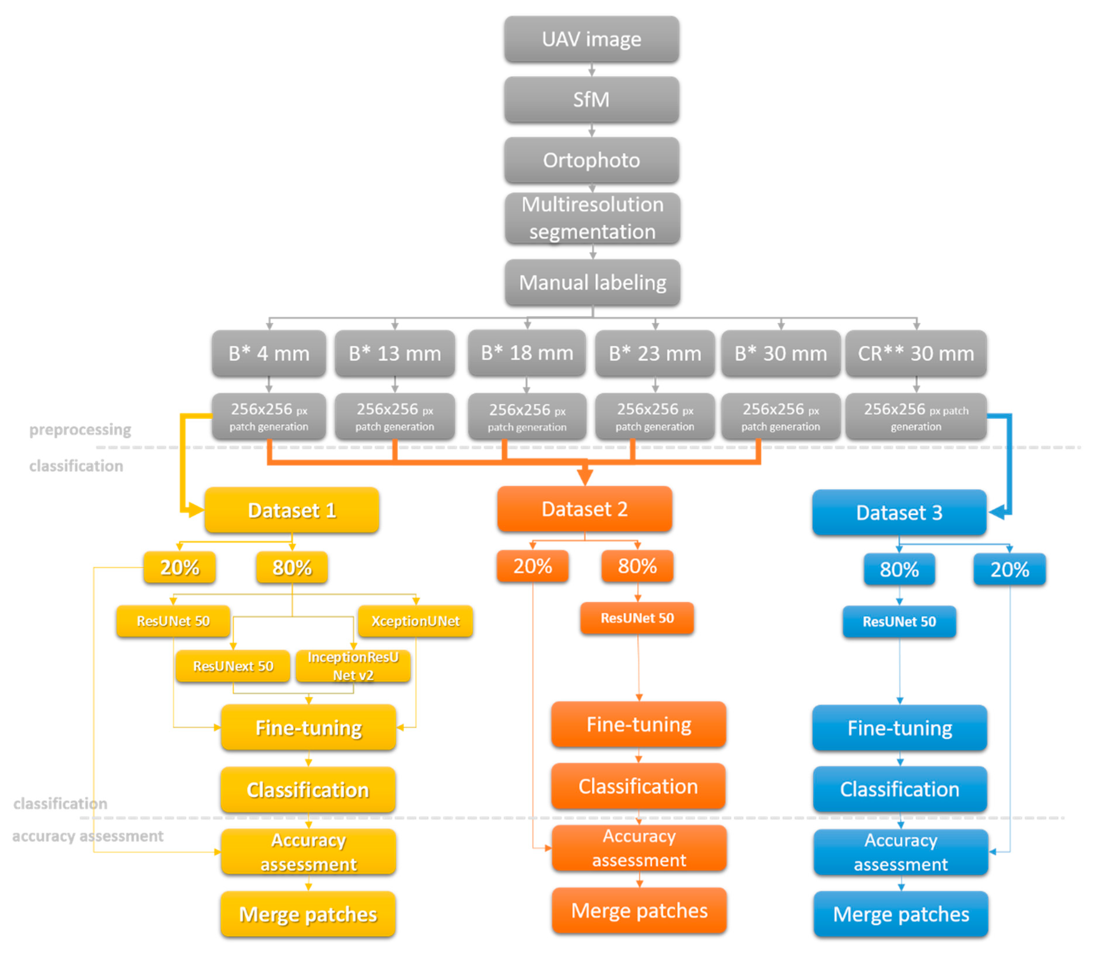
In this paper, a pixel classification method to extract floating plastic pieces from water bodies within VHR remote sensing images based on deep learning algorithms is proposed. Semantic segmentation of floating plastic is highly challenging due to several limitations: low amount of training data, highly imbalanced data sets, limited accuracy of ground truth data, and frequent scene changes due to constant plastic movement. To address those limitations, we propose the workflow showed in Figure 3, which summarizes the approach followed in this paper and consists of three main steps: preprocessing, classification, and accuracy assessment.
4.1. Preprocessing
For each flight, the acquired images and the SfM algorithm were used to generate a high-resolution orthophoto. The SfM algorithm comprises of three main steps [42]: (1) the SIFT algorithm detects and describes key points while the RANdom SAmple Consensus (RANSCAN) method matches key points across multiple images. The bundle block adjustment of matching key points was used to compute the extrinsic and intrinsic camera parameters and three-dimensional (3D) coordinates for a sparse unscaled point cloud; (2) point cloud densification; and (3) digital terrain model and orthophoto generation.
To train the deep learning classifier ground truth data are necessary. Since this study represents the first attempt to map floating plastic based on UAV images, previous ground truth data was not available. Therefore, we created our labels, which was challenging and time consuming, due to the small size, the different colors, the different spectral signatures, the different level of submersion and the constant moving of the floating plastic items.
To reduce the errors caused by the manual delineation of classes, the multiresolution segmentation algorithm implemented in eCognition was used [43]. This algorithm merges pixels to obtain meaningful non-overlapping objects/polygons. The algorithm results are controlled by three factors: (1) scale parameter, i.e., the maximum allowed heterogeneity for the resulting object; (2) shape, i.e., the weight of the object’s shape in comparison to the spectral characteristics of the object (color); and (3) compactness, i.e., the weight representing the compactness of object (please see [43] for more information). The selection of the optimal value combination was based on the trial-and-error process. Each segment was then manually labeled using QGIS software, based on a visual inspection of the orthophoto. In the Balkana study area, plastics were classified into three classes: PET, OPS, and nylon. In the Crna Rijeka area, plastic was classified in two groups: plastic and maybe plastic. The maybe plastic class was created to reduce the spectral confusion in the plastic class, and it was assigned to the segments where the operators were not able to state whether it was plastic by visual inspection and by analyzing the spectral signature.
The Balkana study area was surveyed five times but we were not able to use the same mask for the orthophotos from the different flights (i.e., different spatial resolutions) due to the movement of the plastic. Therefore, for each orthophoto a new ground truth mask was created. This limited the accuracy of the mask and algorithm performance for the lower spatial resolution images.
4.2. Classification
This paper proposes an end-to-end semantic segmentation model for a floating plastic segmentation based on U-net architecture, which has the ability to work with very little training data and provides a precise segmentation [24]. U-Net has a symmetrical encoder-decoder architecture. The encoder side effectively extracts and abstracts the image pixel information while the decoder aims to extract the plastic from the feature maps. The U-Net architecture has been widely used in the semantic segmentation of remote sensing imagery [36,37,38]. Its success is largely attributed to the several skip connections [24,44] between encoding and decoding parts which are used to combine spatial details from lower layers and semantic ones from higher layers of the network. Due to a combination of contextual information at different scales of the input resolution, spatial information can be better restored, producing sharper boundaries of predicted objects after the decoder [45].
4.2.1. Encoder
CNN models consist of a series of layers that are combined in the network. They start with a series of convolutions and a pooling layer, called the convolutional base, and end with a densely connected classifier [46]. The convolutions operate on feature maps with two spatial axes (height and width of the image) and depth (number of channels). The convolutions extract the patches by sliding a window of a fixed size (usually 3 × 3 or 5 × 5) and perform the transformation for all patches, via a dot product with a weight matrix followed by adding bias and the application of the activation function, and finally producing output feature maps [46,47]. The depth of the output feature maps is defined by the number of filters which encode specific aspects of the input data allowing CNN to learn spatial hierarchical patterns. The batch normalization (BN) layer is placed after each convolution to speed up the training process and reduce the internal covariance of each batch of features maps.
The most common way of improving the performance of the deep neural network is increasing the depth (number of layers) and width (number of units within a layer) of the network. However, enlarged networks are more prone to overfitting especially if the size of the training set is limited [48]. Besides, an increase in the network size dramatically increases the use of computational resources.
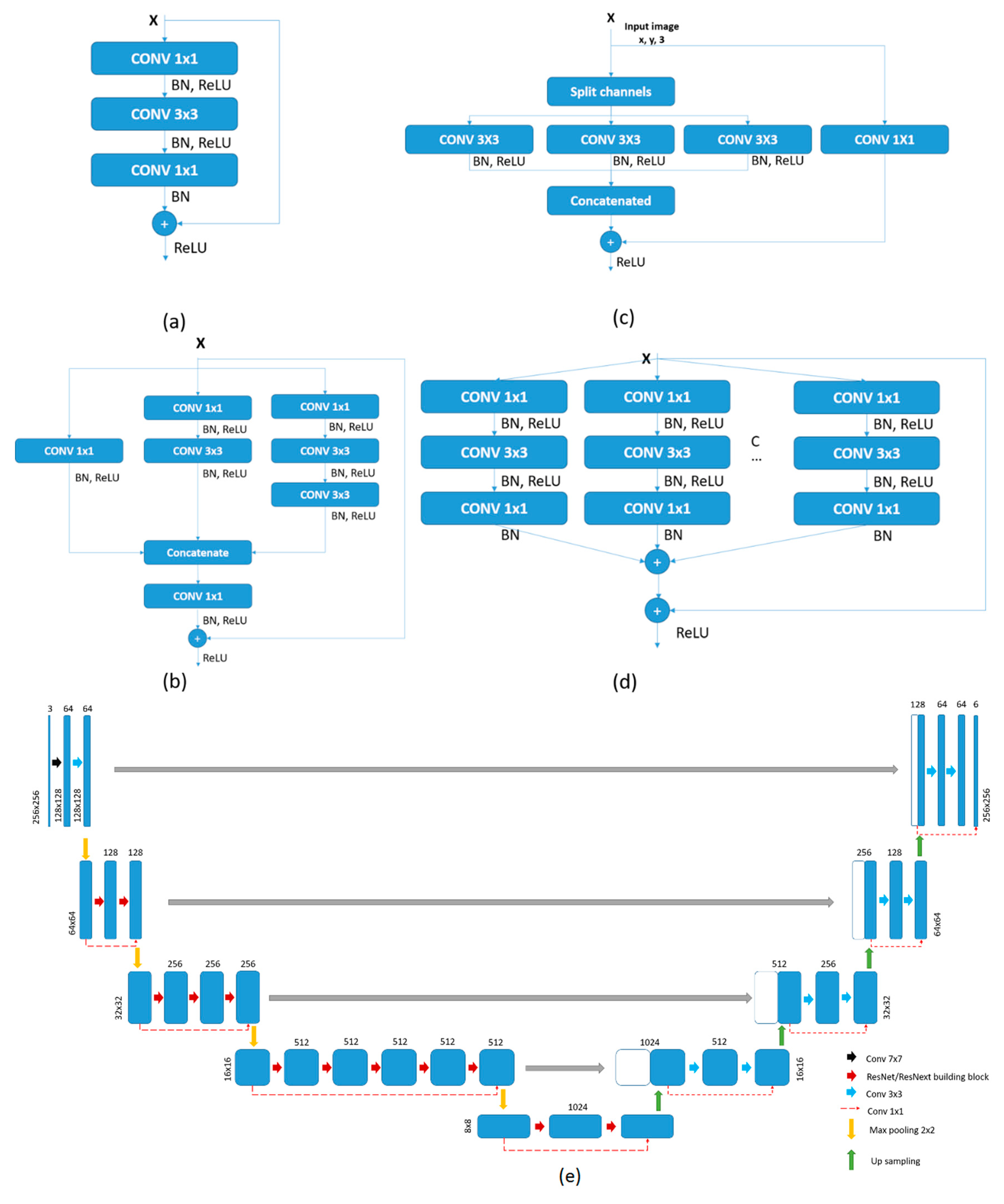
With the increase of the network depth problems like the vanishing gradient start to emerge. The vanishing gradient problem refers to a dramatic gradient decrease as it backpropagates the true network and by the time they reach close to the shallower layers, the updates for the weights nearly vanish. In order to avoid the vanishing gradient problem, a rectified linear unit (ReLU) [49] was used as a nonlinear activation function. The ReLU significantly accelerates the training phase in comparison with the activation functions with a descent gradient such as a sigmoid or hyperbolic tangent function. The pooling layers are used after the convolutional layer to spatially downsample the image and to reduce the number of coefficients to process. Although the stride factor (the distance between two successive windows) can be used for downsampling, the max-pooling tends to work better since it increases the variance by looking at the maximum values of the extracted features over small patches. Since there is not any information about the performance of available models in the case of plastic detection, the encoder side was based on the state of the art CNN models, pre-trained on ImageNet [50] datasets, such as ResNet50 [28], ResNeXt50 [51], Inception-ResNet v2 [30], and Xception [52]. These four architectures were used in this work for the semantic segmentation of floating plastics and are described below.
ResNet50: the deep ResNet architecture addresses the vanishing gradient problem by employing identity skip-connections, which add neither extra parameters nor computational complexity but they lead to a more efficient training and optimization of very deep networks [28]. ResNet is constructed by stacking multiple bottleneck blocks called residual blocks (Figure 4a), which consist of three layers of 1 × 1, 3 × 3, and 1 × 1 convolutions. The 1 × 1 convolution is introduced as the bottleneck layer (to reduce and restore dimensionality) before a 3 × 3 layer to reduce the number of input feature maps and to improve computational efficiency. In this paper, a 50-layer ResNet network was used.
Inception-ResNet v2: this network is constructed by the integration of ResNet [28] and Inception v4 [23], so a residual connection is used to avoid the gradient vanishing problem while the Inception modules increase the network. In the Inception-ResNet v2, the batch normalization is used only on top of the traditional layer enabling the increase of an overall number of Inception blocks [30]. In the Inception blocks, the convolutions with the varying size of the same layer were concatenated at the end of block i.e., the convolution blocks were parallel (Figure 4b). Although the Inception-ResNet v2 shows roughly the same recognition performance as Inception v4, the usage of the residual connection leads to a dramatic improvement in the training speed [30]. Therefore, in this paper, the Inception-ResNet v2 was used.
Xception: the Extremely Inception (Xception) architecture replaces the Inception modules with stacked depthwise separable convolution layers followed by a pointwise convolution. It represents the extreme form of the Inception module, where the spatial features and channel-wise features are fully separated [46]. The Xception architecture has 36 layers structured into 14 modules, all of which have linear residual connections around them, except for the first and last modules (Figure 4c) [52]. The residual connection helps with the vanishing gradient problem both in terms of speed and accuracy.
ResNeXt50: this model is similar to the Inception model since they both follow the split-transform-merge paradigm. However, in the ResNeXt all paths share the same topology and the outputs of different paths are merged by adding them together i.e., ResNeXt consists of a stack of residual blocks that have the same topology (Figure 4d). This architecture introduced the new dimension called cardinality (C) (the number of paths) in addition to depth and width. The results presented in [51] show that an increase in cardinality reduces the error rate while keeping the complexity. In this work a cardinality of 32 was used (Figure 4d).
4.2.2. Decoder
The decoder block aims to upsample the densified encoder (low resolution) feature map to assign a classification result to each pixel of the input image [23]. The encoder and decoder architecture are fully symmetrical i.e., for each encoder there is a corresponding decoder. The decoder gradually recovers the resolution of the original input image by replacing the pooling operation (in the encoder) with 2 × 2 up-sampling operators followed by 3 × 3 convolutions, BN, and the ReLU activation function. The upsampled outputs are combined with contextual information derived from the corresponding encoder via skip connection. In the final layer, a 1 × 1 convolution with the Sigmoid activation function is used to predict the probability of being assigned to one of the pre-defined classes.
4.2.3. Data Augmentation and Transfer Learning
The performance of deep neural networks is highly limited by the low number of training data. The size of the dataset needed for network training is a function of the size of the network (width and depth) and the complexity of the problem. If a model with a large learning capacity is trained on very few data, it can memorize the training sets producing a low generalization power of the model, i.e., overfitting. This overfitting can be reduced by using data augmentation, which artificially enlarges the training set by a random transformation of the existing training samples [26]. Although the produced images are intercorrelated they are not the same, contributing to a better generalization of the network. In addition to reducing overfitting, data augmentation improves the performance when there are imbalanced class problems [53].
Transfer learning is another efficient approach when a limited number of training samples are available. It is based on the idea of fine-tuning (adapting) the models that are already pre-trained on large datasets, such as ImageNet, for completely new classification problems. Transfer learning between different tasks is possible due to the property of deep networks that the first layers are general (i.e., in CNN, first layers tend to learn standard features such as edges, patterns, textures, corners, etc.) while the last layer computes specific features that greatly depend on the chosen dataset and task (such as object parts and objects) [54]. The usual transfer learning approach is based on a fine-tuning which unfreezes (updating weights during the training phase) and adjusts to the parameters of the few top layers in the pre-trained network, while the first layers, representing the general features remain frozen.
4.3. Accuracy Assessment
To test the accuracy of the classification results three standard parameters were calculated: precision, recall, and F-score. Precision (Equation (1)) computes the percent of detected pixels in each class that actually belong to the assigned class, while recall (Equation (2)) represents the fraction of correctly labeled pixels of each class. In a perfect model, the precision and recall are equal to 1. F1-score (Equation (3)) is a quantitative metric useful for imbalanced training data, and it represents the balance between precision and recall [55].
Where TP, FP, FN are true positive, false positive and false negative respectively.
The higher the value of the F1-score, the better the model performance regarding the positive class [56].
4.4. Implementation
Due to the limited processing power, the original images were decomposed to 256 × 256 px patches. The models were based on U-Net architecture, which uses ResNet 50, ResNeXt50, Xception, and Inception-ResNet v2 as encoders. The parameters of the original deep architecture pre-training to the ImageNet datasets were maintained during the fine-tuning. The six different models were trained on three different datasets, as follows. ResNet50, ResNeXt50, Xception, and Inception-ResNet v2 were trained on Dataset 1 (Balkana 4 mm), ResUNet50 was trained on Dataset 2 (which consisted of Balkana 4 mm, 13 mm, 18 mm, 23 mm, and 30 mm resolution orthophotos), and ResUNet was trained on Dataset 3 (Crna Rijeka 30 mm resolution orthophoto) (Figure 3). Dataset 1, Dataset 2, and Dataset 3 contained 328, 434, and 1846 images respectively. All datasets were split into 80% of the data for training and 20% for validation. The batch size was limited by the GPU and it was chosen as big as possible for each network. Different loss functions, such as cross entropy, cross entropy weighted, and focal loss were tested. Since the highest accuracy was obtained using cross entropy, this loss function was used for all the models. The models were implemented in the Python 3 programming language by using artificial intelligence libraries such as PyTorch, TensorFlow, Keras, and Matplotlib. The training of the networks was done using the publicly available cloud platform Colaboratory (Google Colab), which is based on Jupyter Notebooks. The hyperparameters used for the model training are presented in Table 2.
5. Results and Discussion
In this paper, U-Net networks were used for semantic segmentation of floating plastics. Table 3 shows the performance of the four different encoder architectures tested for the extraction of different kinds of plastic materials. Each architecture was pre-trained on the ImageNet datasets and the performance was tested on Dataset 1. Due to simplicity, the results are shown only for the classes that represent plastic.
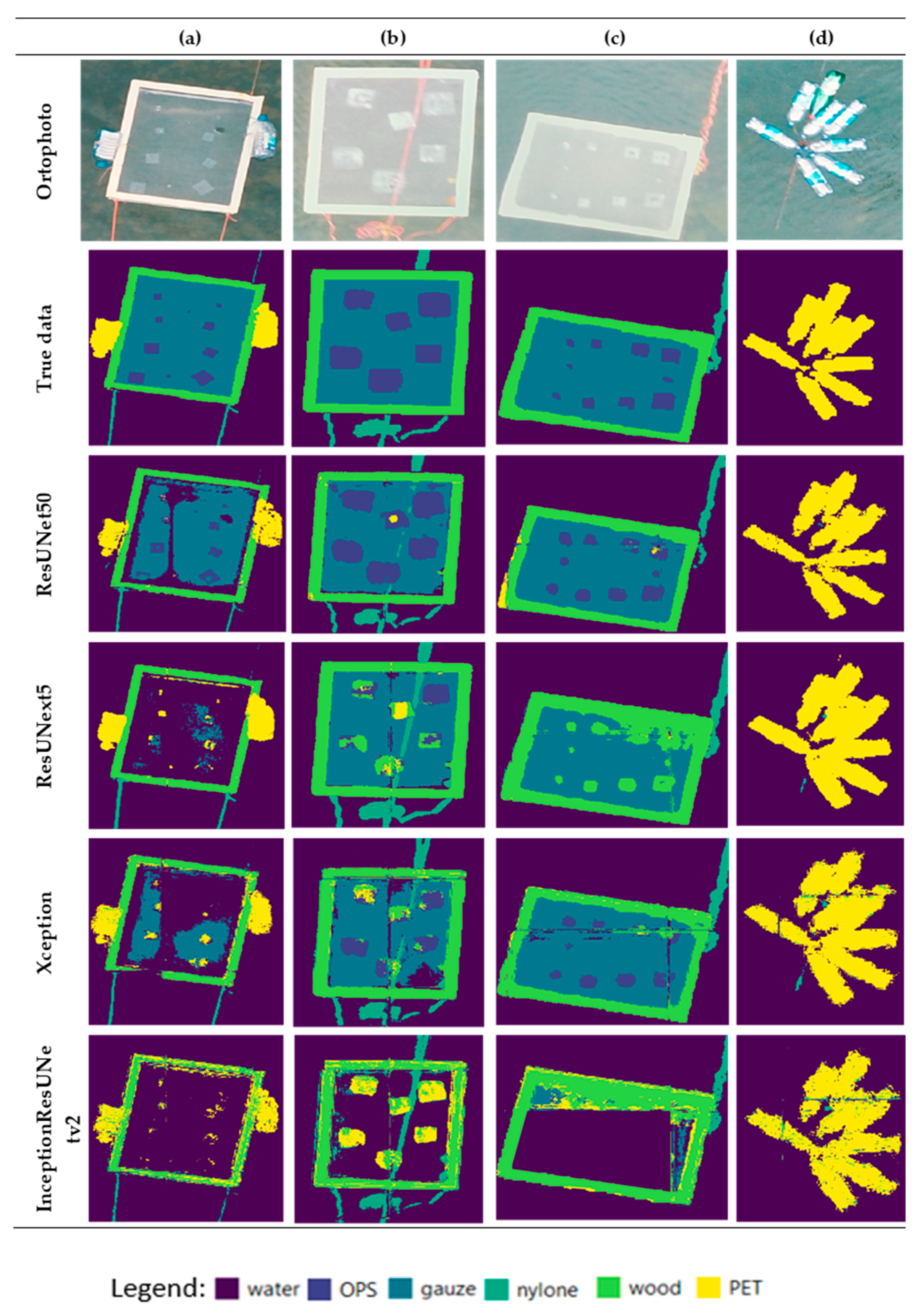
As shown, ResUNet50 has the highest accuracy (F1-score > 0.86) for detecting any of the three plastic classes, while the InceptionResUNet v2 has the lowest (Table 3). Ground truth data and the results of the classification using the four algorithms are shown in Figure 4 for visual inspection (Data set 1). On the one hand, the results show that the ResUNet50 model detected and classified all plastic types with almost no commission or omission errors, matching the ground truth data very accurately (Figure 4 (ResUNet50)). On the other hand, the high recall and low precision obtained by ResUNext50 and XceptionUNet (Table 3.) indicated an overestimation of floating plastic, due to misclassification of water pixels (Figure 4. (ResUNext50, XceptionUNet)). In addition to the misclassification of water pixels, the low accuracy obtained with the InceptionResUNet v2 model (F1: 0; 0.75; 0.65 for each plastic type) was caused by the misclassification between nylon (rope) and PET (bottles), and PET and wood (Figure 4. (InceptionResUNet v2)). The plastic squares were completely omitted by the InceptionResUNet v2, while ResUNext50 strongly misclassified them as wood. On the one hand, the XceptionUNet was capable of detecting small variations in the reflection of different plastic materials (squares F1: 0.53) while, on the other hand, it showed the highest sensitivity to the edge-effect, misclassifying them and decreasing the F1 score. Innamorati et al. [57] showed that segmentation errors are higher for pixels near the edges and even worse at corners [58], due to the lack of the contextual information.
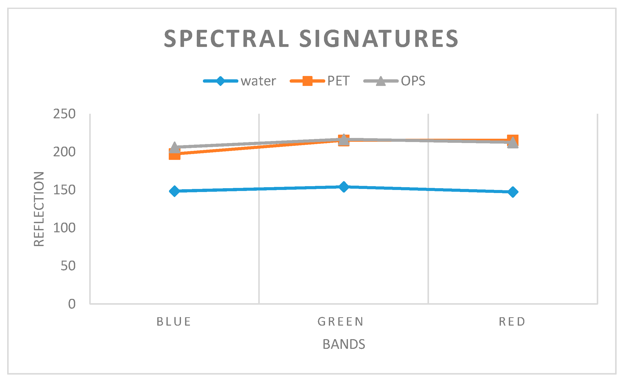
For the underwater squares (Figure 5a), all algorithms, except ResUNet50, misclassified OPS as PET. It should be noted that the total reflection of transparent floating plastic on the water surface is defined as the sum of water reflection, plastic reflection, and the reflection of the light transmitted through the plastic [15,59]. In this study, the presence of plastic bottles (PET) increased, on average, the amount of reflected energy from water by 19%, while OPS increased the reflection by only 3.5% (Figure 6), making it challenging to differentiate between these two classes. This difference is even lower in the case of underwater plastic, due to water absorption, and it can explain the low accuracy of the OPS class for three of the tested models. The quantitative accuracy assessment and the visual inspection confirmed that, among the tested models and for the Lake Balkana study area, ResUNet50 was the most sensitive to detect small differences in the amount of reflected energy, which is crucially important for plastic detection and for identifying different types of plastic. Therefore, all the tests used to achieve the remaining goals of this paper (2, 3, 4) were performed using the ResUNet50 model.
The relationship between the image spatial resolution and the size of the detected plastic was evaluated by using the ResUNet50 model and the ground truth data from Dataset 2. The results of the accuracy assessment are shown in Table 4.
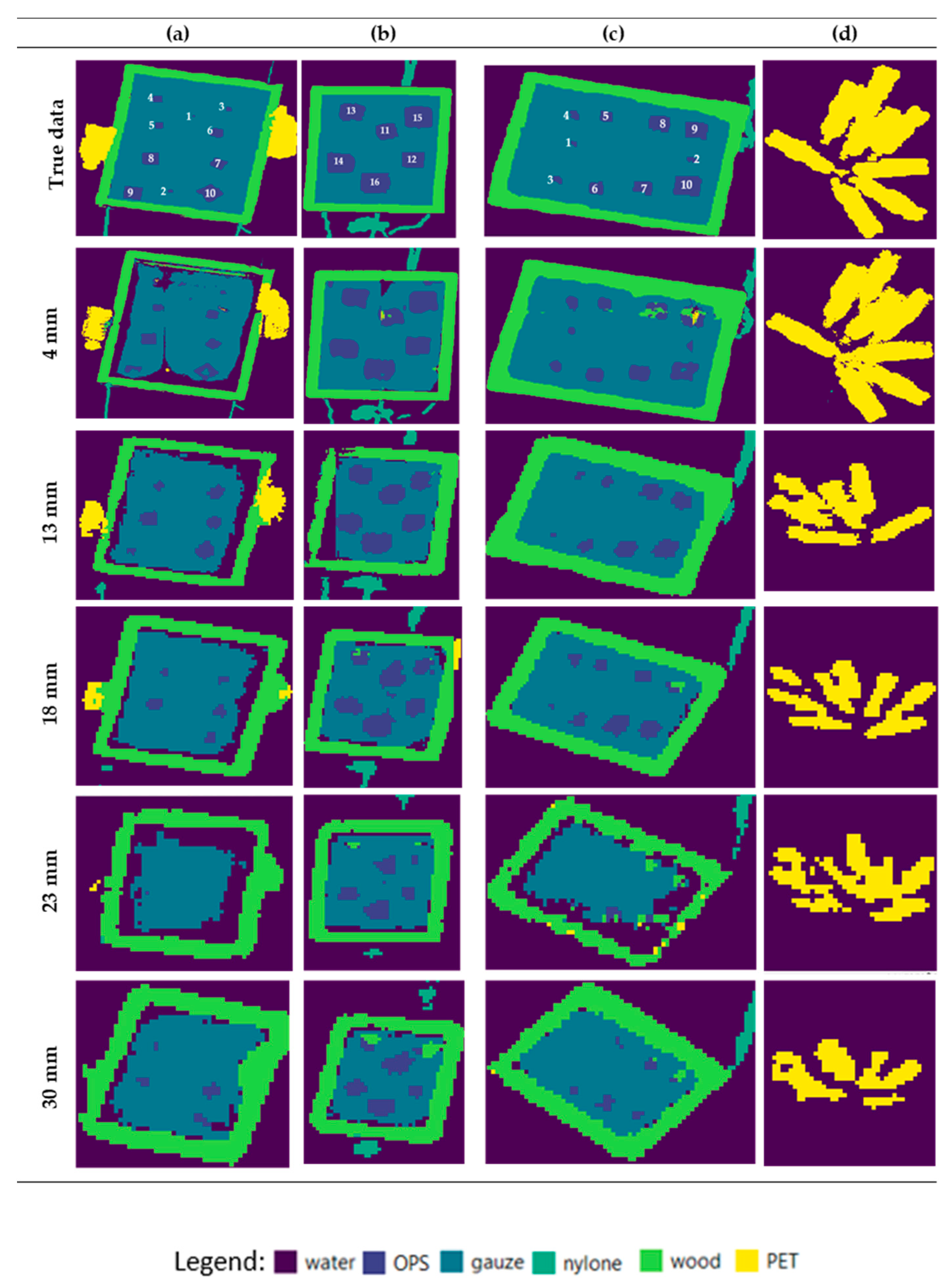
The results showed that the spatial resolution of the image and the accuracy of the model were directly related, i.e., the accuracy decreased with the decrease in spatial resolution. Those findings are in line with the results presented by [60]. As expected, ResUNet50 performed the best on the 4 mm resolution images for all kinds of plastics and the lowest accuracy was obtained for the 30 mm spatial resolution image (Table 4.). The exception was the OPS class, which was mostly omitted in the 23 mm classified orthophoto. Due to changes in of weather conditions (sunny intervals) between the flights, sun glint appeared in the 23 mm orthophoto and increased the reflection [61], in comparison with other images, which led to the misclassification between OPS and gauze (Figure 7 (23 mm), a, b, c), causing the low F1 value. In addition, the amount of reflected energy decreased with the decrease in spatial resolution, due to the larger amount of mixed pixels, resulting in a lower classification accuracy. Visual inspection showed that the algorithm tended to classify mixed pixels as water when the plastic fraction of the target area was larger than the water fraction (e.g., Figure 7d). This result agrees with Ji et. al. [62], who reported that in the case of imbalanced training datasets, mixed pixels tend to be classified as the majority class, even when most of the mixed pixel represents a minority class.
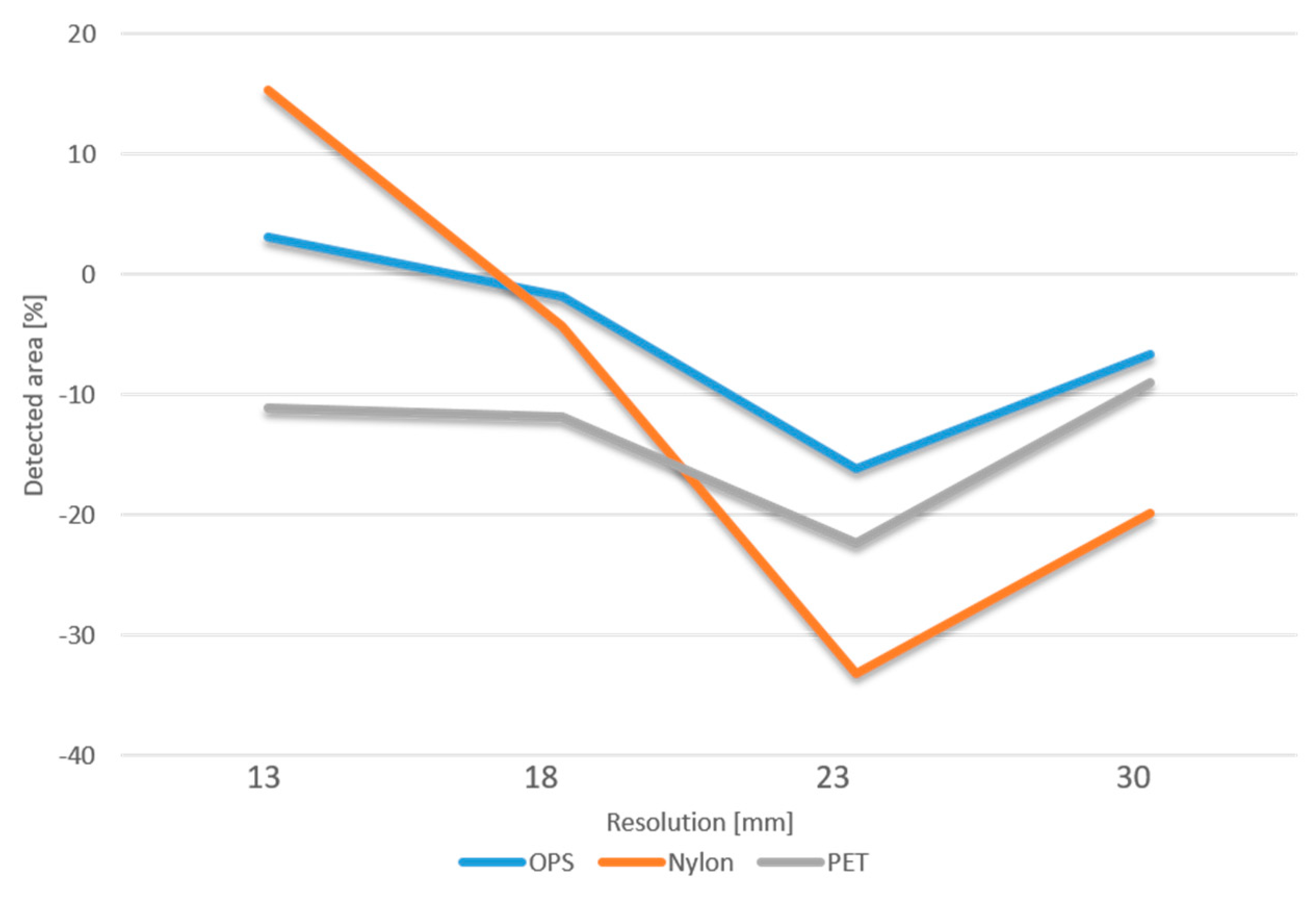
In general, for all the tested spatial resolutions, the algorithm achieved high precision and lower recall values indicating that the model cannot detect all plastic pixels, but that it can be trusted when it does. Taking as a reference value the classification obtained from the 4 mm orthophoto, the largest difference in the extension of the area classified as plastic was obtained from the 23 mm orthophoto (OPS: −16.1%; Nylon: −33.2%; PET: −22.3 %) (Figure 8). The smallest difference for the OPS and Nylon classes was obtained from the 18 mm orthophoto (OPS: −1.8%; Nylon: −4.2%), while the 30 mm orthophoto provided the closest area to the reference for PET plastic (PET: −8.9%) (Figure 7).
The visual inspection showed that with the 4 mm orthophoto the algorithm detected all the OPS squares, while with the 13 mm and 18 mm orthophotos the algorithm omitted the 1 and 2 cm squares on the water surface, and the 1 to 4 cm squares that were underwater. For the 23 mm image, it omitted all the OPS squares smaller than 11 cm, while for 30 mm image, the 1 to 4 cm squares, which were on the water surface, and the 1 to 6 cm squares located underwater, were misclassified as water (Figure 7). Based on these results it can be concluded that the algorithm needs at least one pure pixel (a pixel that includes a single surface material) for detecting plastics on the water surface, and two pure pixels for the detection of underwater plastics. According to the presented results, orthophotos with of 18 mm spatial resolution can be used for litter surveys which follow OSPAR [9], NOAA [11] or UNEP/IOC [12] guidelines, while 4 mm orthophotos should be used for CSIRO [10] surveys, since according to CSIRO guidelines, the minimum size of detected plastic should be 1 cm2.
On the one hand, floating plastic is more accurately extracted from images with higher spatial resolution. On the other hand, the higher the spatial resolution of the image, the smaller the extension of the area covered by the image, as showed in Figure 9. Therefore, a compromise between spatial resolution and the covered area needs to be found.
To test the model performance in an independent scenario, the Crna Rijeka study area was surveyed. Based on the size of the study area and the size of the majority of the plastic items (bottles) that were present, a 30 mm orthophoto was used (Dataset 3), as well as the ResUNet50 model. The results of the accuracy assessment are presented in Table 5.
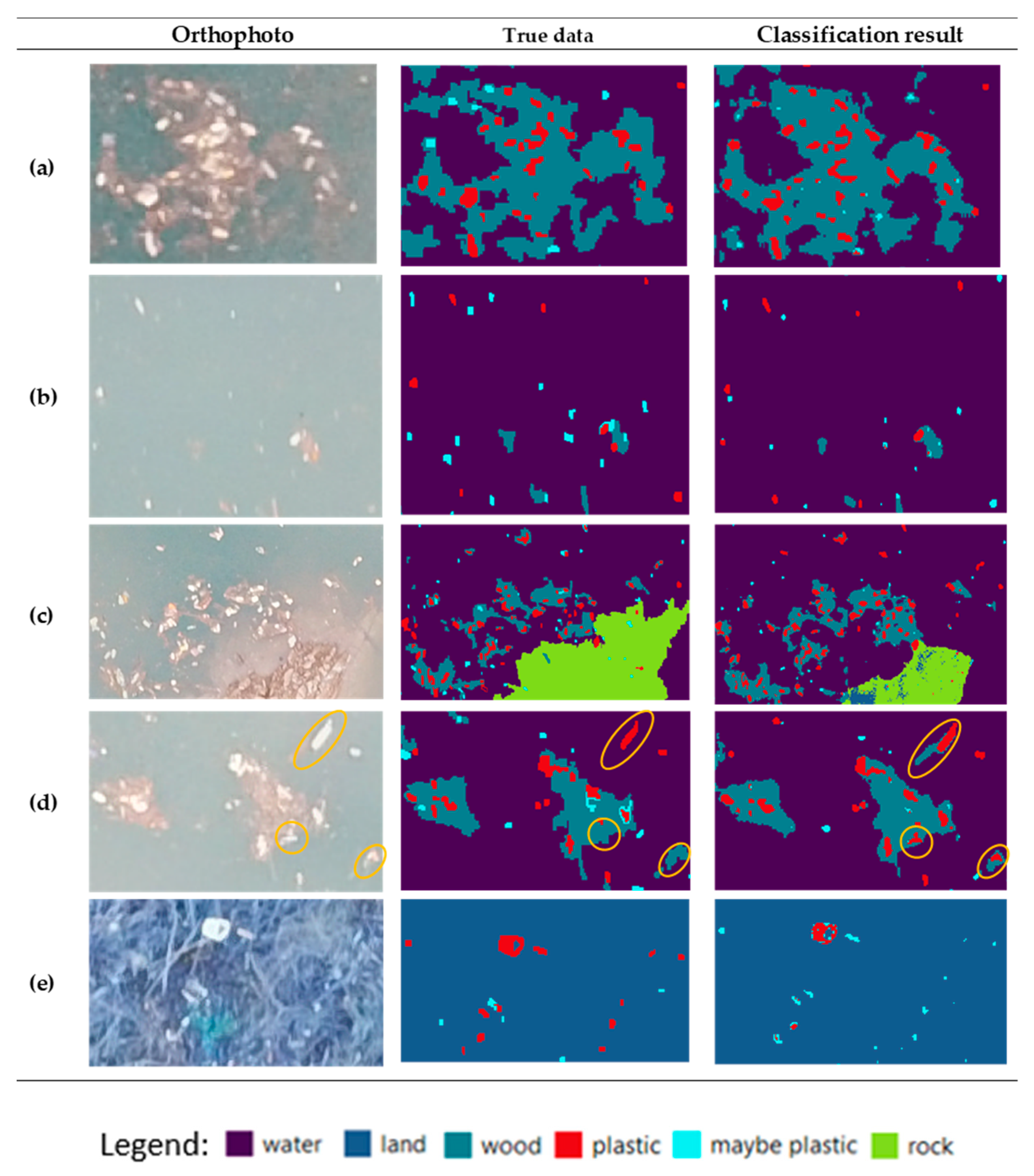
The ResUNet50 showed a stable performance to classify plastic in the different datasets (Dataset 2 (PET class) and Dataset 3 (plastic class)) when comparing the same spatial resolution (F1: 0.73 vs. 0.78, respectively) (Table 4 and Table 5). The highest confusion was obtained for the “maybe plastic” class, which was misclassified as water or plastic. For that class the precision was high, while recall was low, indicating the underestimation of the area covered by the maybe plastic class. Although precision, recall, and F1 score provide a deeper insight into the performance of the algorithm, the area and volume of the detected plastics are more useful for stakeholders. From an operational point of view, when planning a cleaning campaign, that information is the basis for site selection, and for estimating the number of people required and the approximate time needed. In the Crna Rijeka case study, the algorithm only underestimated the plastic area by 3.4%, proving the great potential of its application to optimize cleaning campaigns.
The visual inspection shows (Figure 10) that the locations of the plastic pieces were accurately detected, but some plastic pixels on the border were misclassified as the surrounding class. No differences were observed in the performance of the model between grouped (Figure 10a) or single plastic items (Figure 10b).
Unexpectedly, the algorithm detected plastic accurately in shallow water (Figure 10c). Shallow water is highly challenging for mapping plastic because the presence of the river bed increases water reflectance (same as plastic does) [15]. In this study case, the algorithm accurately extracted the plastic pieces that were omitted from the training data (Figure 10d), showing good generalization abilities, Moreover, the model showed its potential for plastic detection not just in water but also on land, with lower accuracy compared with the floating plastics (Figure 10e).
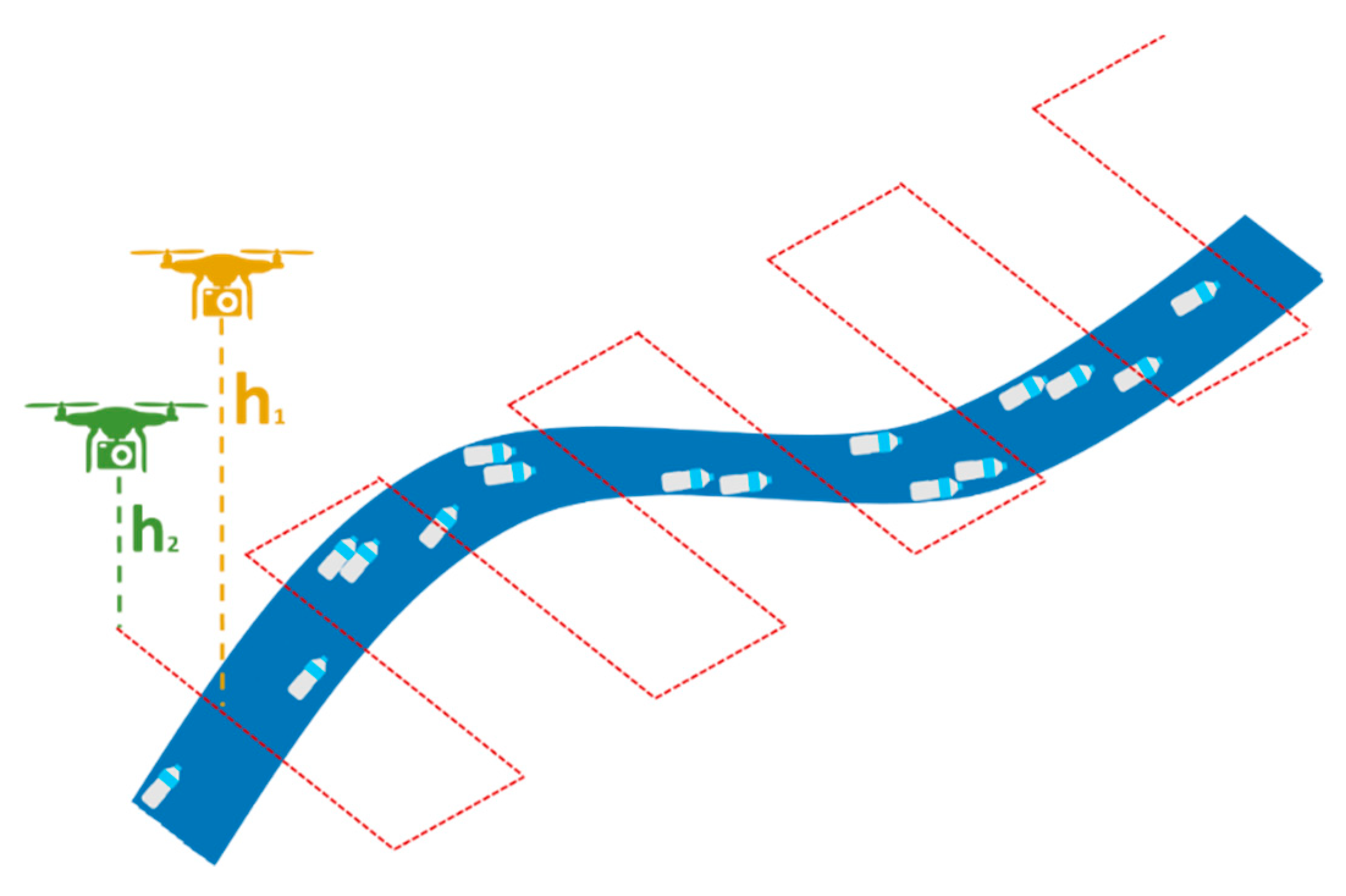
It should be also taken into account that the results are also affected by the accuracy of the training data. The creation of training data was time consuming and a tedious task. Just in the case of the Crna Rijeka orthophoto (Dataset 3), the 418,542 segments were manually labeled, assigning 5519 to the plastic class and 4014 to the maybe plastic one. Visual labeling of plastic pieces is a difficult task which involves errors due to the limited ability to exactly determine the boundary between plastic and maybe plastic. Therefore, in the case of misclassifications between those two classes, it cannot be stated if it was an error in the algorithms or if it was due to a misclassification during the manual labeling stage. To address this limitation, we suggest that during the collection of training data, two UAVs with the same flight pattern should be used (Figure 11). The first UAV would fly at a higher altitude while the second UAV would fly lower to provide higher resolution images which can be used for precise delineation and labeling of the plastic class and other classes, to therefore obtain an accurate data mask. Since floating plastic moves continuously, especially on windy days, the speed of the second UAV should be lower than the first one, to synchronize their flight missions and reduce time overlap between surveys.
Moreover, the UAV surveys should be carried out during cloudy weather to reduce the sunglint effect, since it limits the quality and accuracy of remote sensing data from water bodies [61]. Anggoro et al. [63] reported that the reduction of the sunglint effect increased the overall accuracy by 7%. The same accuracy degradation of was noted in the classification of the 23 mm orthophoto (Table 4.; Figure 7 (23 mm)). Also, the wind speed should be as low as possible, especially in the case of small UAVs. The stability of the camera is affected by the wind and it can cause blurred imagery. In addition, the SfM reconstructs a 3D point cloud based on the matching of multiple views, so if the plastic pieces shift their relative position from image-to-image due to wind-induced movements, the reliability of the point cloud and the accuracy of the produced orthophoto is compromised.
6. Conclusions
Automatic floating plastic extraction from high-resolution UAV orthophotos can be accurately achieved using the end-to-end semantic segmentation ResUNet50 algorithm. Among the other tested algorithms, ResUNet50 showed a stable performance to detect and classify floating plastic in the different datasets and for different spatial resolutions, for underwater and floating targets (F1 score > 0.73). The ResUNext50 and XceptionUNet models led to an overestimation of the floating plastic due to misclassification of water pixels. The model also showed its suitability for plastic detection on water, shallow water and also on land, with lower accuracy compared with the floating plastics. An underestimation of the plastic area of only 3.4% showed its utility to monitor plastic pollution effectively and makes it possible to use it to optimize cleaning campaigns, as well as the integration and comparison of the estimations.
It was possible to accurately detect and classify the three different plastic types located in the study area (OPS, PET, Nylon) using the ResUNet50 model (F1: OPS: 0.86; Nylon: 0.88; PET: 0.92), which was the most sensitive to detect small differences in the amount of reflected energy.
Regarding the relationship between spatial resolution and detectable plastic size, the classification accuracy decreased with the decrease in spatial resolution, performing best on 4 mm resolution images for all the different kinds of plastic. The model cannot detect all plastic pixels, but it can be trusted when it does, for all the tested spatial resolutions. Moreover, the algorithm needs at least one pure plastic pixel (a pixel that only contains that material) to detect plastics on the water surface, and two pure pixels for the detection of underwater plastics. The results obtained with the 18 mm spatial resolution orthophotos and the proposed method meet the requirements described in OSPAR [9], NOAA [11] or UNEP/IOC [12] guidelines, while CSIRO [10] surveys will require the use of 4 mm orthophotos.
Taking as a reference value the classification obtained for the 4 mm orthophoto, the largest difference in the extension of the area classified as plastic was obtained using the 23 mm orthophoto (OPS: 16.1%; Nylon: 33.2%; PET: 22.3 %) (Figure 8). The smallest difference for the OPS and Nylon classes was obtained using the 18 mm orthophoto (OPS: 1.8%; Nylon: 4.2%), while the 30 mm orthophoto provided the closest area to the reference for PET plastic (PET: 8.9%) (Figure 8).
When planning a UAV survey to map floating plastic, the following issues should be taking into account: (i) reaching a compromise between the spatial resolution and the area covered by each image, (ii) two UAVs with the same flight pattern should be used, one to collect the imagery to obtain the maps and a second one flying lower than the other, so it can capture very high spatial resolution data to delineate an accurate training dataset, (iii) synchronizing the two flight missions and reduce time overlap between surveys, (iv) flying during cloudy weather to reduce the sunglint effect, and (v) wind speed should be as low as possible, so the quality of the orthophoto is not compromised.
Author Contributions
Conceptualization, G.J., M.G., and F.A.-T.; methodology, G.J. and M.G.; software, G.J.; validation, G.J; formal analysis, G.J, M.G., and F.A.-T.; investigation, G.J.; writing—original draft preparation, G.J. and M.G.; writing—review and editing, G.J., M.G., and F.A.-T.; visualization, G.J.; supervision M.G. and F.A.-T. All authors have read and agreed to the published version of the manuscript.
Funding
This research received no external funding.
Acknowledgments
The authors would like to thank the three anonymous reviewers who helped improve the manuscript with their comments and suggestions.
Conflicts of Interest
The authors declare no conflict of interest.
References
- Plastics Europe. Available online: https://www.plasticseurope.org/application/files/9715/7129/9584/FINAL_web_version_Plastics_the_facts2019_14102019.pdf (accessed on 27 April 2020).
- United Nations Environment Program. Available online: https://www.unenvironment.org/news-and-stories/press-release/un-declares-war-ocean-plastic-0 (accessed on 27 April 2020).
- United Nations Environment Program. The state of plastic. Available online: https://wedocs.unep.org/bitstream/handle/20.500.11822/25513/state_plastics_WED.pdf?isAllowed=y&sequence=1 (accessed on 27 April 2020).
- Lebreton, L.; van der Zwet, J.; Damsteeg, J.W.; Slat, B.; Andrady, A.; Reisser, J. River plastic emissions to the world’s oceans. Nat. Commun. 2017, 8, 15611. [Google Scholar] [CrossRef] [PubMed]
- Jambeck, J.R.; Hardesty, B.D.; Brooks, A.L.; Friend, T.; Teleki, K.; Fabres, J.; Beaudoin, Y.; Bamba, A.; Francis, J.; Ribbink, A.J.; et al. Challenges and emerging solutions to the land-based plastic waste issue in Africa. Mar. Policy 2018, 96, 256–263. [Google Scholar] [CrossRef]
- The guardian. Available online: https://www.theguardian.com/science/2017/nov/05/terrawatch-the-rivers-taking-plastic-to-the-oceans (accessed on 27 April 2020.).
- Eriksen, M.; Lebreton, L.C.M.; Carson, H.S.; Thiel, M.; Moore, C.J.; Borerro, J.C.; Galgani, F.; Ryan, P.G.; Reisser, J. Plastic pollution in the world’s oceans: More than 5 trillion plastic pieces weighing over 250,000 tons afloat at sea. PLoS ONE 2014, 9, e111913. [Google Scholar] [CrossRef] [PubMed] [Green Version]
- Jambeck, J.R.; Geyer, R.; Wilcox, C.; Siegler, T.R.; Perryman, M.; Andrady, A.; Narayan, R.; Law, K.L. Plastic waste inputs from land into the ocean. Science 2015, 347, 768–771. [Google Scholar] [CrossRef]
- OSPAR commission. Guideline for Monitoring Marine Litter on the Beaches in the OSPAR Monitoring Area. Available online: https://www.ospar.org/documents?v=7260 (accessed on 22 April 2020).
- Hardesty, B.D.; Lawson, T.J.; van der Velde, T.; Lansdell, M.; Wilcox, C. Estimating quantities and sources of marine debris at a continental scale. Front. Ecol. Environ. 2016, 15, 18–25. [Google Scholar] [CrossRef]
- Opfer, S.; Arthur, C.; Lippiatt, S. NOAA Marine Debris Shoreline Survey Field Guide, 2012. Available online: https://marinedebris.noaa.gov/sites/default/files/ShorelineFieldGuide2012.pdf (accessed on 25 April 2020).
- Cheshire, A.C.; Adler, E.; Barbière, J.; Cohen, Y.; Evans, S.; Jarayabhand, S.; Jeftic, L.; Jung, R.T.; Kinsey, S.; Kusui, E.T.; et al. UNEP/IOC Guidelines on Survey and Monitoring of Marine Litter. UNEP Regional Seas Reports and Studies 2009, No. 186; IOC Technical Series No. 83: xii + 120 pp. Available online: https://www.nrc.govt.nz/media/10448/unepioclittermonitoringguidelines.pdf (accessed on 25 April 2020).
- Ribic, C.A.; Dixon, T.R.; Vining, I. Marine Debris Survey Manual. Noaa Tech. Rep. Nmfs 1992, 108, 92. [Google Scholar]
- Kooi, M.; Reisser, J.; Slat, B.; Ferrari, F.F.; Schmid, M.S.; Cunsolo, S.; Brambini, R.; Noble, K.; Sirks, L.-A.; Linders, T.E.W.; et al. The effect of particle properties on the depth profile of buoyant plastics in the ocean. Sci. Rep. 2016, 6, 33882. [Google Scholar] [CrossRef] [Green Version]
- Jakovljevic, G.; Govedarica, M.; Alvarez Taboada, F. Remote Sensing Data in Mapping Plastic at Surface Water Bodies. In Proceedings of the FIG Working Week 2019 Geospatial Information for A Smarter Life and Environmental Resilience, Hanoi, Vietnam, 22–26 April 2019. [Google Scholar]
- Aoyama, T. Extraction of marine debris in the Sea of Japan using high-spatial resolution satellite images. In SPIE Remote Sensing of the Oceans and Inland Waters: Techniques, Applications, and Challenges; SPIE—International Society for Optics and Photonics: New Delhi, India, 2016. [Google Scholar] [CrossRef]
- Gray, P.C.; Fleishman, A.B.; Klein, D.J.; McKown, M.W.; Bezy, V.S.; Lohmann, K.J.; Jhonston, D.W. A Convolutional Neural Network for Detecting Sea Turtles in Drone Imagery. Methods Ecol. Evol. 2018, 10, 345–355. [Google Scholar] [CrossRef]
- Hong, S.-J.; Han, Y.; Kim, S.-Y.; Lee, A.-Y.; Kim, G. Application of Deep-Learning Methods to Bird Detection Using Unmanned Aerial Vehicle Imagery. Sensors 2019, 19, 1651. [Google Scholar] [CrossRef] [Green Version]
- Martin, C.; Parkes, S.; Zhang, Q.; Zhang, X.; McCabe, M.F. Use of unnamed aerial vehicle for efficient beach litter monitoring. Mar. Pollut. Bull. 2018, 131, 662–673. [Google Scholar] [CrossRef] [Green Version]
- Topouzelis, K.; Papakonstantinou, A.; Garaba, S.P. Detection of floating plastics from satellite and unmanned aerial systems (Plastic Litter Project 2018). Int. J. Appl. Earth Obs. Geoinf. 2019, 79, 175–183. [Google Scholar] [CrossRef]
- Geraeds, M.; van Emmeric, T.; de Vries, R.; bin Ab Razak, M.S. Riverine Plastic Litter Monitoring Using Unmanned Aerial Vehicles (UAVs). Remote Sens. 2019, 11, 2045. [Google Scholar] [CrossRef] [Green Version]
- Moy, K.; Neilson, B.; Chung, A.; Meadows, A.; Castrence, M.; Ambagis, S.; Davidson, K. Mapping coastal marine debris using aerial imagery and spatial analysis. Mar. Pollut. Bull. 2018, 132, 52–59. [Google Scholar] [CrossRef] [PubMed]
- Boonpook, W.; Tan, Y.; Ye, Y.; Torteeka, P.; Torsri, K.; Dong, S. A Deep Learning Approach on Building Detection from Unmanned Aerial Vehicle-Based Images in Riverbank Monitoring. Sensors 2018, 18, 3921. [Google Scholar] [CrossRef] [Green Version]
- Ronneberger, O.; Fischer, P.; Brox, T. U-Net: Convolutional Networks for Biomedical Image Segmentation. arXiv 2015, arXiv:1505.04597v1. Available online: https://arxiv.org/abs/1505.04597 (accessed on 25 April 2020.).
- Schmidt, C.; Krauth, T.; Wagner, S. Export of Plastic Debris by Rivers into the Sea. Environ. Sci. Technol. 2017, 51, 12246–12253. [Google Scholar] [CrossRef]
- Krizhevsky, A.; Sutskever, I.; Hinton, G.E. ImageNet classification with deep convolutional neural networks. In Proceedings of the Advances in Neural Information Processing Systems, Lake Tahoe, ND, USA, 3–6 December 2012; pp. 1097–1105. [Google Scholar]
- Simonyan, K.; Zisserman, A. Very Deep Convolutional Networks for Large-Scale Image Recognition. arXiv 2014, arXiv:1409.1556. [Google Scholar]
- He, K.; Zhang, X.; Ren, S.; Sun, J. Deep residual learning for image recognition. In Proceedings of the IEEE Conference on Computer Vision and Pattern Recognition, Las Vegas, NV, USA, 26 June–1 July 2016; pp. 770–778. [Google Scholar]
- Huang, G.; Liu, Z.; van der Maaten, L.; Weinberger, K.Q. Densely Connected Convolutional Networks. 2016, arXiv:1608.06993. Available online: https://arxiv.org/abs/1608.06993 (accessed on 25 April 2020).
- Szegedy, C.; Ioffe, S.; Vanhoucke, V.; Alemi, A.A. Inception-4, Inception-ResNet and the impact of residual connections on learning. In Proceedings of the Thirty-First AAAI Conference on Artificial Intelligence, San Francisco, CA, USA, 4–10 February 2017. [Google Scholar]
- Song, H.S.; Kim, Y.H.; Kim, Y.I. A Patch-Based Light Convolutional Neural Network for Land-Cover Mapping Using Landsat-8 Images. Remote Sens. 2019, 11, 114. [Google Scholar] [CrossRef] [Green Version]
- Lagkvist, M.; Kiselev, A.; Alirezaie, M.; Loutfi, A. Classification and Segmentation of Satellite Orthoimagery Using Convolutional Neural Networks. Remote Sens. 2016, 8, 329. [Google Scholar] [CrossRef] [Green Version]
- Long, J.; Shelhamer, E.; Darrell, T. Fully Convolutional Networks for Semantic Segmentation. In Proceedings of the IEEE Conference on Computer Vision and Pattern Recognition, Boston, MA, USA, 7–12 June 2015; pp. 3431–3440. [Google Scholar]
- Yu, F.; Koltun, V. Multi-scale context aggregation by dilated convolution. arXiv 2016, arXiv:1511.07122. Available online: https://arxiv.org/abs/1511.07122 (accessed on 25 April 2020).
- Chen, L.-C.; Papandreou, G.; Kokkinos, I.; Murphy, K.; Yuille, A.L. Deeplab: Semantic image segmentation with deep convolutional nets, Atrous convolution, and fully connected CRFs. IEEE Trans. Pattern Anal. Mach. Intell. 2018, 40, 834–848. [Google Scholar] [CrossRef] [PubMed]
- Zhao, X.; Yuan, Y.; Song, M.; Ding, Y.; Lin, F.; Liang, D.; Zhang, D. Use of Unmanned Aerial Vehicle Imagery and Deep Learning UNet to Extract Rice Lodging. Sensors 2019, 19, 3859. [Google Scholar] [CrossRef] [Green Version]
- Xu, Y.; Wu, L.; Xie, Z.; Chen, Z. Building Extraction in Very High Resolution Remote Sensing Imagery Using Deep Learning and Guided Filters. Remote Sens. 2018, 10, 144. [Google Scholar] [CrossRef] [Green Version]
- Yi, Y.; Zhang, Z.; Zhang, W.; Zhang, C.; Li, W.; Zhao, T. Semantic Segmentation of Urban Buildings from VHR Remote Sensing Imagery Using a Deep Convolutional Neural Network. Remote Sens. 2019, 11, 1774. [Google Scholar] [CrossRef] [Green Version]
- Guo, H.; He, G.; Jiang, W.; Yin, R.; Yan, L.; Leng, W. A Multi-Scale Water Extraction Convolutional Neural Network (MWEN) Method for GaoFen-1 Remote Sensing Images. Isprs Int. J. Geo Inf. 2020, 9, 189. [Google Scholar] [CrossRef] [Green Version]
- Pashaei, M.; Kamangir, H.; Starek, M.J.; Tissot, P. Review and Evaluation of Deep Learning Architectures for Efficient Land Cover Mapping with UAS Hyper-Spatial Imagery: A Case Study Over a Wetland. Remote Sens. 2020, 12, 959. [Google Scholar] [CrossRef] [Green Version]
- Ekocentar Bočac. Available online: https://ekocentar-bocacjezero.com/zastitna_mreza/zaustavljanje-plutajuceg-otpada-na-mrezi/ (accessed on 29 February 2020).
- Govedarica, M.; Jakovljević, G.; Taboada, F.A. Flood risk assessment based on LiDAR and UAV points clouds and DEM. In Proceedings of the SPIE 10783, Remote Sensing for Agriculture, Ecosystems, and Hydrology XX, 107830B, Berlin, Germany, 10 October 2018. [Google Scholar] [CrossRef]
- Trimble. Available online: http://www.ecognition.com/ (accessed on 12 January 2020).
- Zhou, Z.; Siddiquee, M.R.; Tajbakhsh, N.; Liang, J. UNet++: Redesigning Skip Connections to Exploit Multiscale Features in Image Segmentation. IEEE Trans. Med. Imaging. 2020. Available online: https://arxiv.org/pdf/1912.05074.pdf (accessed on 27 April 2020). [CrossRef] [Green Version]
- Wang, Y.; Liang, B.; Ding, M.; Li, J. Dense Semantic Labeling with Atrous Spatial Pyramid Pooling and Decoder for High-Resolution Remote Sensing Imagery. Remote Sens. 2019, 11, 20. [Google Scholar] [CrossRef] [Green Version]
- Chollet, F. Deep Learning with Python; Manning Publications Co.: Greenwich, CT, USA, 2017. [Google Scholar]
- Goodfellow, I.; Bengio, Y.; Courville, A. Deep Learning. The MIT Press: Cambridge, MA, USA, 2016. [Google Scholar]
- Szegedy, C.; Liu, W.; Jia, Y.; Sermanet, P.; Reed, S.; Anguelov, D.; Erhan, D.; Vanhoucke, V.; Rabinovich, A. Going Deeper with Convolutions. In Proceedings of the IEEE Conference on Computer Vision and Pattern Recognition, Boston, MA, USA, 7–12 June 2015; pp. 1–9. [Google Scholar] [CrossRef] [Green Version]
- Nair, V.; Hinton, G.E. Rectified Linear Units Improve Restricted Boltzmann Machines. In Proceedings of the 27th International Conference on Machine Learning, Haifa, Israel, 21–24 June 2010. [Google Scholar]
- Deng, J.; Dong, W.; Socher, R.; Li, L.; Li, K.; Fei-Fei, L. ImageNet: A large-scale hierarchical image database. In Proceedings of the IEEE Conference on Computer Vision and Pattern Recognition, Miami, FL, USA, 20–25 June 2009; pp. 248–255. [Google Scholar]
- Xie, S.; Girshick, R.; Dollar, P.; Tu, Z.; He, K. Aggregated Residual Transformations for Deep Neural Network. In Proceedings of the IEEE Conference on Computer Vision and Pattern Recognition (CVPR), Honolulu, HI, USA, 21–26 July 2017; Available online: https://arxiv.org/abs/1611.05431 (accessed on 25 April 2020).
- Chollet, F. Xception: Deep Learning with Depthwise Separable Convolutions. In Proceedings of the IEEE Conference on Computer Vision and Pattern Recognition (CVPR), Honolulu, HI, USA, 21–26 July 2017; pp. 1251–1258. [Google Scholar]
- Hasini, R.; Shokri, M.; Dehghan, M. Augmentation Scheme for Dealing with Imbalanced Network Traffic Classification Using Deep Learning. arXiv 2019, arXiv:1901.00204. Available online: https://arxiv.org/pdf/1901.00204.pdf (accessed on 25 April 2020).
- Yosinski, J.; Clune, J.; Bengio, Y.; Lipson, H. How transferable are features in deep neural networks? In Advances in Neural Information Processing Systems 27 (NIPS ’14); NIPS Foundation: Montreal, QC, Canada, 2014. [Google Scholar]
- Fawcett, T. An introduction to ROC analysis. Pattern Recognit. Lett. 2006, 27, 861–874. [Google Scholar] [CrossRef]
- Bekkar, M.; Kheliouane Djemaa, H.; Akrouf Alitouche, T. Evaluation Measure for Models Assessment over Imbalanced Data Sets. J. Inf. Eng. Appl. 2013, 3, 27–38. [Google Scholar]
- Innamorati, C.; Ritschel, T.; Weyrich, T.; Mitra, N.J. Learning on the Edge: Explicit Boundary Handling in CNNs. arXiv 2018, arXiv:180503106.2018. Available online: https://arxiv.org/pdf/1805.03106.pdf (accessed on 25 April 2020).
- Cui, Y.; Zhang, G.; Liu, Z.; Xiong, Z.; Hu, J. A Deep Learning Algorithm for One-step Contour Aware Nuclei Segmentation of Histopathological Images. Med. Biol. Eng. Comput. 2019, 57, 2027–2043. [Google Scholar] [CrossRef] [Green Version]
- Goddijn-Murphy, L.; Peters, S.; van Sebille, E.; James, N.; Gibb, S. Concept for a hyperspectral remote sensing algorithm for floating marine macro plastics. Mar. Pollut. Bull. 2018, 126, 255–262. [Google Scholar] [CrossRef] [PubMed] [Green Version]
- Kannoji, S.P.; Jaiswal, G. Effects of Varying Resolution on Performance of CNN based Image Classification: An Experimental Study. Int. J. Comput. Sci. Eng. 2018, 6, 451–456. [Google Scholar] [CrossRef]
- Kay, S.; Hedley, J.; Lavender, S. Sun Glint Correction of High and Low Spatial Resolution Images of Aquatic Scenes: A Review of Methods for Visible and Near-Infrared Wavelengths. Remote Sens. 2009, 1, 697–730. [Google Scholar] [CrossRef] [Green Version]
- Ji, L.; Gong, P.; Geng, X.; Zhao, Y. Improving the Accuracy of the Water Surface Cover Type in the 30 m FROM-GLC Product. Remote Sens. 2015, 7, 13507–13527. [Google Scholar] [CrossRef] [Green Version]
- Anggoro, A.; Siregar, V.; Agus, S. The effect of sunglint on benthic habitats mapping in Pari Island using worldview-2 imagery. Procedia Environ. Sci. 2016, 33, 487–495. [Google Scholar] [CrossRef] [Green Version]
Figure 1.
Study areas: Lake Balkana (left) and Crna Rijeka River (right). EPSG:3857.

Figure 2.
Targets used in the study area located in Lake Balkana (a) frame with metal construction for the underwater survey, (b) frame for the on the water surface survey, (c) nylon rope, (d) plastic bottles.
Figure 2.
Targets used in the study area located in Lake Balkana (a) frame with metal construction for the underwater survey, (b) frame for the on the water surface survey, (c) nylon rope, (d) plastic bottles.

Figure 3.
Workflow used in this study where “B*” and “CR**” correspond with the Balkana and Crna Rijeka dataset respectively. UAV = Unmanned Aerial Vehicles; SfM = Structure from Motion.
Figure 3.
Workflow used in this study where “B*” and “CR**” correspond with the Balkana and Crna Rijeka dataset respectively. UAV = Unmanned Aerial Vehicles; SfM = Structure from Motion.

Figure 4.
Building blocks of (a) ResNet, (b) Inception-ResNet v2, (c) Xception, and (d) ResNeXt (C = 32) (e) architecture of ResUNet50/ResUNext50. Where: ReLu is Rectified Linear Unit, BN is Batch Normalization, and CONV is convolution.
Figure 4.
Building blocks of (a) ResNet, (b) Inception-ResNet v2, (c) Xception, and (d) ResNeXt (C = 32) (e) architecture of ResUNet50/ResUNext50. Where: ReLu is Rectified Linear Unit, BN is Batch Normalization, and CONV is convolution.

Figure 5.
Ground truth data and results of the classification using the four tested models for detecting different plastic materials, located underwater (a) and overwater (b–d) (Dataset 1). Where: OPS is Oriented Polystyrene and PET is Polyethylene terephthalate.
Figure 5.
Ground truth data and results of the classification using the four tested models for detecting different plastic materials, located underwater (a) and overwater (b–d) (Dataset 1). Where: OPS is Oriented Polystyrene and PET is Polyethylene terephthalate.

Figure 6.
Spectral signatures of water, PET and OPS.

Figure 7.
Ground truth data and results of the classification using the ResUNet50 algorithm for visual comparison, at different spatial resolutions and for different plastic materials, located underwater (a) and overwater (b–d) (Dataset 2).
Figure 7.
Ground truth data and results of the classification using the ResUNet50 algorithm for visual comparison, at different spatial resolutions and for different plastic materials, located underwater (a) and overwater (b–d) (Dataset 2).

Figure 8.
Differences in the extension of the detected area covered by plastic (using the classification of the 4 mm orthophoto as a reference value).
Figure 8.
Differences in the extension of the detected area covered by plastic (using the classification of the 4 mm orthophoto as a reference value).

Figure 9.
Relationship between the spatial resolution (cm/pixel) and the area covered by an image gathered by the DJI Mavic ProCamera (grid mission with an 80 % overlap).
Figure 9.
Relationship between the spatial resolution (cm/pixel) and the area covered by an image gathered by the DJI Mavic ProCamera (grid mission with an 80 % overlap).

Figure 10.
Visual comparison between the orthophoto, true data (ground truth) and classification results for the five different scenarios: (a) group of plastics, (b) single plastic items, (c) plastic in shallow waters, (d) training data errors (orange lines), which were misclassified by the operator and correctly classified by the algorithm (e) plastic on the ground.

Figure 11.
Proposed flight planning methodology to obtain accurate datasets for algorithm calibration.
Figure 11.
Proposed flight planning methodology to obtain accurate datasets for algorithm calibration.


Table 1.
Flight heights and spatial resolutions of the conducted surveys.
| Flight Height (m) | Spatial Resolution (mm) | |
|---|---|---|
| Balkana | Crna Rijeka | |
| 12 | 4 | - |
| 40 | 13 | - |
| 55 | 18 | - |
| 70 | 23 | - |
| 90 | 30 | 30 |
Table 2.
Hyperparameters used for training the models.
| Study Area | Dataset | Architecture | Batch Size | Learning Rate | Training Time |
|---|---|---|---|---|---|
| Balkana | Dataset 1 | ResUNet50 | 8 | 8 × 10⁻⁵ | 31 min |
| Balkana | Dataset 1 | ResUNext50 | 8 | 1 × 10⁻⁶ | 44 min |
| Balkana | Dataset 1 | XceptionUNet | 8 | 2 × 10⁻⁵ | 21 min |
| Balkana | Dataset 1 | InceptionUResNet v2 | 8 | 1 × 10⁻⁵ | 33 min |
| Balkana | Dataset 2 | ResUNet50 | 8 | 3 × 10⁻⁵ | 40 min |
| Crna Rijeka | Dataset 3 | ResUNet50 | 8 | 4 × 10⁻⁶ | 3 h |
Table 3.
Comparison of different encoder architectures for floating plastic detection (where P, R, F1, are precision, recall, and F1-score respectively) (Dataset 1).
Table 3.
Comparison of different encoder architectures for floating plastic detection (where P, R, F1, are precision, recall, and F1-score respectively) (Dataset 1).
| ResUNet50 | ResUNext50 | XceptionUNet | InceptionResUNet v2 | |||||||||
|---|---|---|---|---|---|---|---|---|---|---|---|---|
| P | R | F1 | P | R | F1 | P | R | F1 | P | R | F1 | |
| OPS | 0.86 | 0.86 | 0.86 | 0.99 | 0.19 | 0.31 | 0.81 | 0.39 | 0.53 | 0.01 | 0.00 | 0.00 |
| Nylon | 0.92 | 0.85 | 0.88 | 0.77 | 0.96 | 0.85 | 0.76 | 0.87 | 0.81 | 0.76 | 0.74 | 0.75 |
| PET | 0.92 | 0.92 | 0.92 | 0.82 | 0.96 | 0.88 | 0.78 | 0.75 | 0.77 | 0.60 | 0.72 | 0.65 |
Table 4.
The effect of spatial resolution (mm) on ResUNet50 performance (where P, R, F1 are precision, recall, and F1-score respectively) (Dataset 2).
Table 4.
The effect of spatial resolution (mm) on ResUNet50 performance (where P, R, F1 are precision, recall, and F1-score respectively) (Dataset 2).
| 13 mm | 18 mm | 23 mm | 30 mm | |||||||||
|---|---|---|---|---|---|---|---|---|---|---|---|---|
| P | R | F1 | P | R | F1 | P | R | F1 | P | R | F1 | |
| OPS | 0.88 | 0.77 | 0.82 | 0.69 | 0.71 | 0.70 | 0.79 | 0.31 | 0.44 | 0.75 | 0.45 | 0.56 |
| Nylon | 0.89 | 0.75 | 0.82 | 0.91 | 0.52 | 0.66 | 0.76 | 0.26 | 0.39 | 0.87 | 0.20 | 0.33 |
| PET | 0.92 | 0.83 | 0.87 | 0.78 | 0.84 | 0.81 | 0.83 | 0.68 | 0.75 | 0.77 | 0.70 | 0.73 |
Table 5.
Precision, Recall, and F1-score of plastic classes in the Crna Rijeka study area.
| Precision | Recall | F1 | |
|---|---|---|---|
| Plastic | 0.82 | 0.75 | 0.78 |
| Maybe Plastic | 0.62 | 0.34 | 0.43 |
© 2020 by the authors. Licensee MDPI, Basel, Switzerland. This article is an open access article distributed under the terms and conditions of the Creative Commons Attribution (CC BY) license (http://creativecommons.org/licenses/by/4.0/).
Share and Cite
MDPI and ACS Style
Jakovljevic, G.; Govedarica, M.; Alvarez-Taboada, F. A Deep Learning Model for Automatic Plastic Mapping Using Unmanned Aerial Vehicle (UAV) Data. Remote Sens. 2020, 12, 1515. https://0-doi-org.brum.beds.ac.uk/10.3390/rs12091515
AMA Style
Jakovljevic G, Govedarica M, Alvarez-Taboada F. A Deep Learning Model for Automatic Plastic Mapping Using Unmanned Aerial Vehicle (UAV) Data. Remote Sensing. 2020; 12(9):1515. https://0-doi-org.brum.beds.ac.uk/10.3390/rs12091515
Chicago/Turabian StyleJakovljevic, Gordana, Miro Govedarica, and Flor Alvarez-Taboada. 2020. "A Deep Learning Model for Automatic Plastic Mapping Using Unmanned Aerial Vehicle (UAV) Data" Remote Sensing 12, no. 9: 1515. https://0-doi-org.brum.beds.ac.uk/10.3390/rs12091515
Note that from the first issue of 2016, this journal uses article numbers instead of page numbers. See further details here.