An Improved Cloud Detection Method for GF-4 Imagery

Abstract

Clouds are significant barriers to the application of optical remote sensing images. Accurate cloud detection can help to remove contaminated pixels and improve image quality. Many cloud detection methods have been developed. However, traditional methods either rely heavily on thermal infrared bands or clear-sky images. When traditional cloud detection methods are used with Gaofen 4 (GF-4) imagery, it is very difficult to separate objects with similar spectra, such as ice, snow, and bright sand, from clouds. In this paper, we propose a new method, named Real-Time-Difference (RTD), to detect clouds using a pair of images obtained by the GF-4 satellite. The RTD method has four main steps: (1) data preprocessing, including transforming digital value (DN) to Top of Atmosphere (TOA) reflectance, and orthographic and geometric correction; (2) the computation of a series of cloud indexes for a single image to highlight clouds; (3) the calculation of the difference between a pair of real-time images in order to obtain moved clouds; and (4) confirming the clouds and background by analyzing their physical and dynamic features. The RTD method was validated in three sites located in the Hainan, Liaoning, and Xinjiang areas of China. The results were compared with those of a popular classifier, Support Vector Machine (SVM). The results showed that RTD outperformed SVM; for the Hainan, Liaoning, and Xinjiang areas, respectively, the overall accuracy of RTD reached 95.9%, 94.1%, and 93.9%, and its Kappa coefficient reached 0.92, 0.88, and 0.88. In the future, we expect RTD to be developed into an important means for the rapid detection of clouds that can be used on images from geostationary orbit satellites.

1. Introduction

The Gaofen 4 (GF-4) satellite (gaofen is the Chinese for “high resolution”) was launched on 29 December 2015 and is the first Chinese optical remote sensing satellite in geostationary orbit that was specifically designed for civil use [1]. A panchromatic multispectral sensor (PMS) and an infrared sensor (IRS) are on board the GF-4 satellite. An individual GF-4 scene can cover an area of 400 km × 400 km, with a spatial resolution of about 50 m and 400 m for the PMS and IRS, respectively [2]. GF-4 was designed to operate in gazing image mode, and thus the revisit period can reach 20 s [3]. GF-4 can obtain a series of time-continuous images over the same area, which provides an ideal observation approach for the detection of changing and moving targets. Therefore, GF-4 data can play a significant role in various applications, such as disaster reduction [4], forestry, seismology, meteorology, and marine surveillance [5]. Recently, many applications have been performed based on GF-4 imagery, such as radiometric cross-calibration [6], the acquisition of super-resolution images [2], ship tracking [7], and the recognition of residential areas [8].

Clouds are significant barriers to the application of GF-4 remote sensing data since they obscure a large amount of important information about the Earth’s surface [9]. For most remote sensing applications, such as vegetation monitoring [10], land-cover and land-use analysis [11], change detection [12], and multi-temporal data fusion [13], it is necessary to first detect and exclude clouds before further image processing. Therefore, cloud detection has been one of the most important issues since remote sensing data were first produced [14,15]. In recent years, a great number of excellent cloud detection methods have been proposed. These methods can be roughly divided into two categories based on how many images are used: single-image-based methods and multi-temporal-based methods [16].

Single-image-based methods use a single satellite image to detect clouds. These methods commonly include physical-rule-based approaches and machine-learning-based approaches [17]. Physical-rule-based approaches detect clouds according to the physical characteristics of clouds. Clouds are generally bright, cold, white, and high. As such, in imagery they present higher brightness values in the visible, near-infrared, and shortwave infrared bands, lower values in the thermal infrared bands, and higher elevations and flatter reflectance across the optical bands than most ground objects. Most physical-rule-based algorithms use some predefined or adaptive thresholds derived from physical rules to identify clouds [18]. The performances of several cloud-detection algorithms that use only a single image have been investigated by previous studies. Among these methods, Function of Mask (Fmask) [19] obtained the highest accuracy when a thermal band was required [20]. Of the methods which do not require a thermal band, the automated cloud-cover assessment (ACCA) method [21] performs the best [20]. Recently, Fmask was further developed into version 4.0. Additionally, Global Surface Water Occurrence (GSWO) data and a global Digital Elevation Model (DEM) were used as auxiliary data, and a new Spectral-Contextual Snow Index (SCSI) was further proposed to better distinguish ice and snow from clouds [16].

Machine-learning-based approaches detect clouds based on statistics of spatial and spectral features. In general, such approaches require a large number of training samples, a classifier, and some features to be used in the classification [22]. The whole cloud-detection process can commonly be separated into three stages: training, calculation, and validation. In the first stage, a large number of training samples are needed to train some features through classifiers. In the second stage, the classifiers and above-learned features are used to classify the whole image. Finally, some random samples are used to validate the method’s accuracy. The cloud-detection problem can be formulated as a classification problem and solved using classification models, such as Decision Trees [23], Neural Networks (NN) [24], Support Vector Machines (SVM) [25,26], etc. In recent years, Convolutional Neural Networks (CNN) have obtained high accuracy and achieved great success in the field of cloud detection since they can convolve the entire input image to obtain multi-level spatial and spectral features [22,24].

Multi-temporal cloud-detection methods are also referred to as real-time cloud detection or temporal differencing. Such methods calculate the difference between two images that were acquired at different times (a current image and a previous image); those pixels whose spectral characteristics changed significantly between the images will be identified as clouds [27]. Multi-temporal cloud-detection methods are based on the hypothesis that clouds are always dynamic, and the presence of a cloud will lead to a sudden change in reflectance. Therefore, temporal changes between images can be used to easily detect clouds. Liu et al. proposed an inflexion-based cloud-detection algorithm to generate cloud masks from a time series of MOD09 products [28]. When time series of reflectance are assembled together, inflexion points will exist between the cloudy and clear-sky observations, and those areas with reflectance values larger than the inflexion will be identified as cloudy [28]. Zhu and Woodcock proposed an algorithm called multi-temporal mask (Tmask). This algorithm fits a time series model of each pixel using remaining clear pixels based on an initial cloud mask from Fmask. Then, it compares model estimates of cloud cover with observations in the time series to detect cloud pixels that were omitted in the initial screening by Fmask [11]. In general, multi-temporal methods are better at detecting clouds than single-image methods, as the temporal information provides a valuable complement to spectral information, which is very important for distinguishing clouds from clear land surfaces [29].

However, these methods cannot be fully applicable to GF4 data since there was no thermal band equipped on the payload. It is difficult to estimate the temperature, like Landsat data, to distinguish clouds and snow. Furthermore, it is challenging to obtain clear-sky GF-4 imagery in cloudy areas for use in multi-temporal cloud detection. Therefore, some other features of clouds in GF-4 satellite imagery should be explored. This is because GF-4 is a geostationary orbit satellite with gazing image mode and can capture many images of an area in a short time. By analyzing these images, the movement of clouds can be clearly observed. In this study, we developed a new cloud detection method for use with GF-4 imagery, which is called the Real-Time-Difference (RTD) method. The RTD method was developed and tested using GF-4 images from three sites, in the Hainan, Liaoning, and Xinjiang areas of China. Additionally, the performance of the method was compared with that of an SVM machine-learning method.

2. Materials

The GF-4 satellite can provide fast, reliable, and stable optical images for many applications, such as disaster reduction, forestry, seismology, and meteorology, and also has great potential in industries such as environmental protection, marine, agriculture, and water conservation, as well as regional applications. In recent years, GF-4 imagery has attracted significant research interest due to its continuous imaging properties [2,5]. The orbit parameters and the technical indicators of the GF-4 satellite payload are given in

Table 1. Orbit parameters of the Gaofen-4 (GF-4) satellite.

Parameter	Indicator
Orbit type	Geosynchronous orbit
Orbit altitude	36,000 km
Fixed point location	105.6°E

and

Table 2. Technical indicators of the GF-4 satellite payload.

Spectral Band No.	Spectral Range (µm)	Spatial Resolution (m)	Breadth (km)	Revisit Time (s)
1	0.45~0.90	50	400	20
2	0.45~0.52	50	400	20
3	0.52~0.60	50	400	20
4	0.63~0.69	50	400	20
5	0.76~0.90	50	400	20
6	3.50~4.10	400	400	20

, respectively.

2.1. Test Images

(1)

Hainan area

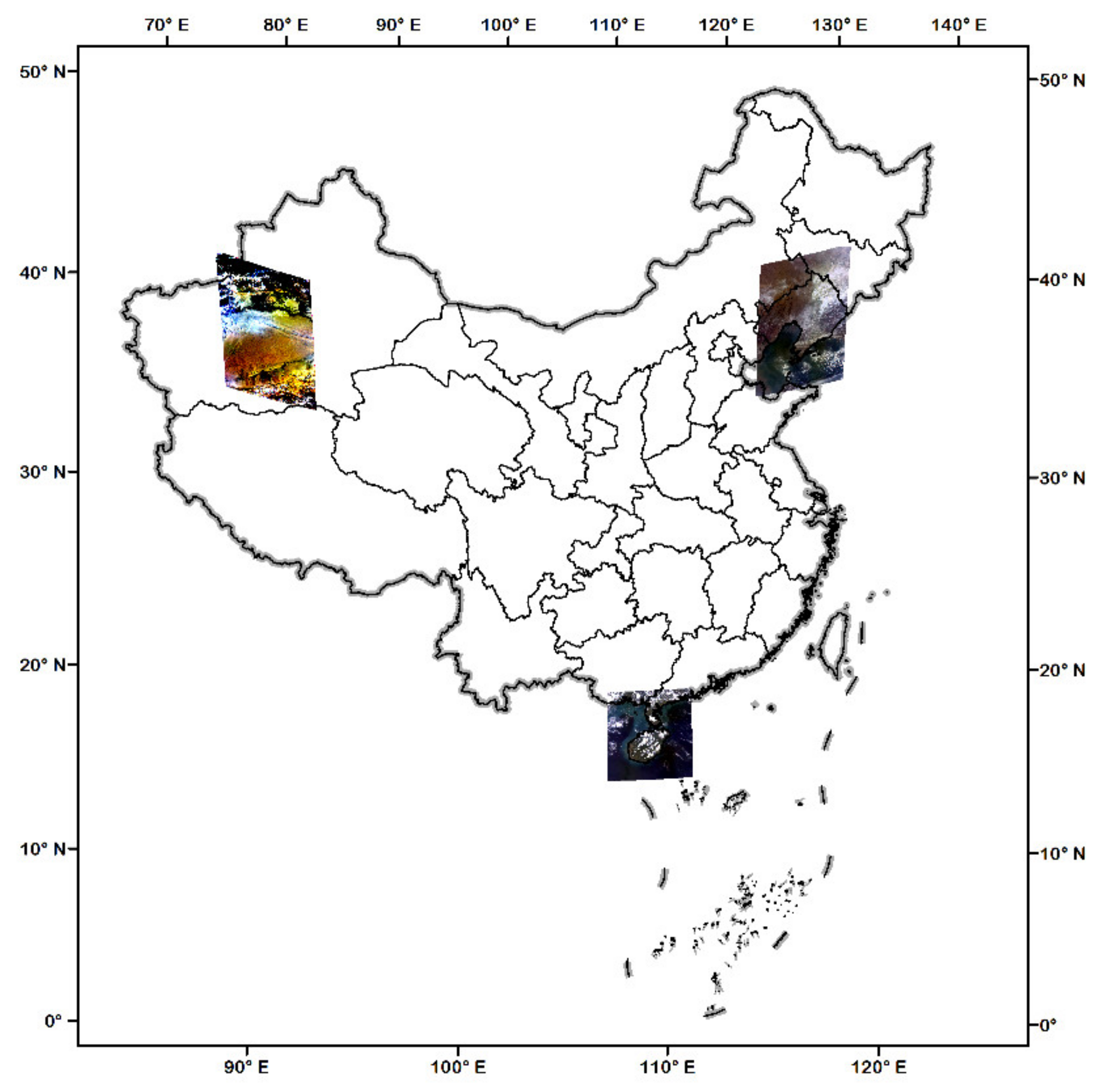
In order to validate the effectiveness of the RTD method, we selected a study area in Hainan Province. This site contains water and a large amount of land and has highly complex water and land backgrounds. Two GF-4 images of this area were used, which were centered at 19.72°N and 109.93°E and captured at 5:30:21 and 5:41:29 GMT on 20 August 2016. These data were freely downloaded from the China Center for Resources Satellite Data and Application (www.cresda.com). The locations of the test sites in China are shown in Figure 1.

(2)

Liaoning area

Ice and snow on the land surface greatly complicate cloud detection due to the fact that their spectra are similar to those of clouds; many cloud detection methods have difficulty in separating these features. Current cloud detection methods mainly rely on thermal and cirrus bands to derive temperature, and it is very difficult to distinguish clouds when these bands are not available. In order to test the effectiveness of the RTD method in areas with ground ice and snow, we selected the Liaoning area as another study area. Two GF-4 images centered at 40.93°N and 122.73°E and captured at 3:04:04 and 3:05:13 GMT on 08 January 2017 were used. The GF-4 images were freely downloaded from the China Center for Resources Satellite Data and Application. At the time of acquisition, there was a large amount of ice and snow cover on the land surface in this area, and these images can therefore be used to test the effectiveness of the RTD method.

(3)

Xinjiang area

In order to further evaluate the effectiveness of the RTD method, we selected Xinjiang as another study area due to the presence of many snowy mountains. Two GF-4 images obtained at 11:51:54 and 11:54:13 GMT on 22 September 2018 were used.

2.2. Reference Images

A total of 30 reference images were used in this experiment to train a series of threshold parameters that were used in the experiment. These reference images are evenly distributed in most geographic regions of China. A total of 2 or 3 images were randomly selected in each geographic region. A variety of surface types, such as forest, grassland, farmland, desert, snowy mountain, built-up area, and ocean, were covered in these reference images. The acquisition times of these images were also different. These reference images are listed in

Table 3. The reference data used in this experiment.

Dataset ID
GF4_PMS_E91.2_N37.9_20181119_L1A0000223392	GF4_PMS_E93.5_N27.2_20180405_L1A0000191705
GF4_PMS_E95.7_N37.8_20181119_L1A0000223393	GF4_PMS_E101.4_N23.3_20180715_L1A0000203338
GF4_PMS_E102.5_N31.9_20180720_L1A0000204513	GF4_PMS_E102.6_N27.7_20180720_L1A0000204512
GF4_PMS_E114.8_N27.0_20181122_L1A0000223800	GF4_PMS_E122.7_N45.6_20180405_L1A0000191701
GF4_PMS_E124.8_N27.6_20180715_L1A0000203347	GF4_PMS_E112.4_N18.6_20181201_L1A0000224692
GF4_PMS_E84.1_N38.7_20180830_L1A0000214112	GF4_PMS_E100.2_N37.8_20181119_L1A0000223394
GF4_PMS_E110.9_N36.4_20180720_L1A0000204522	GF4_PMS_E115.3_N36.4_20180720_L1A0000204521
GF4_PMS_E118.3_N27.7_20180719_L1A0000203560	GF4_PMS_E128.3_N45.9_20180405_L1A0000191702
GF4_PMS_E108.8_N18.5_20181201_L1A0000224693	GF4_PMS_E108.9_N22.3_20181201_L1A0000224698
GF4_PMS_E109.1_N30.2_20181128_L1A0000224373	GF4_PMS_E110.2_N15.5_20181122_L1A0000223841
GF4_PMS_E123.2_N32.1_20180720_L1A0000204518	GF4_PMS_E106.6_N36.4_20180720_L1A0000204523
GF4_PMS_E108.8_N23.3_20180715_L1A0000203336	GF4_PMS_E109.5_N40.8_20180715_L1A0000203368
GF4_PMS_E111.3_N30.3_20180707_L1A0000201956	GF4_PMS_E114.1_N23.4_20180713_L1A0000203186
GF4_PMS_E114.7_N31.9_20180720_L1A0000204516	GF4_PMS_E118.9_N32.0_20180720_L1A0000204517
GF4_PMS_E86.6_N26.9_20170817_L1A0000171808	GF4_PMS_E119.5_N38.7_20170303_L1A0000156660

.

2.3. Auxiliary Data

The main auxiliary data used in the RTD method were Global Surface Water Occurrence (GSWO) data. The GSWO dataset provides terrestrial water dynamics (intra- and interannual variability and change) over long time periods at a spatial resolution of 30 m and was produced based on a 32 year Landsat record [16,30]. The dataset provides water occurrence for each pixel, where 0% indicates permanent land and 100% indicates permanent water [16].

2.4. Validation Data

To validate the accuracy of the proposed RTD method, a standard cloud mask was derived from manual visual interpretation of the test images. The clouds were manually constructed in the ArcMap 10.6 software based on the observation of the original satellite images. However, there are some limitations to the manual cloud mask, in that it is sometimes very difficult for the human eye to distinguish whether a pixel corresponds to a cloud or not, especially for optically thin and fragmented clouds scattered over a city or inshore ocean. Therefore, a total of 2000 pixels, including 1000 cloud pixels and 1000 background pixels, were selected based on stratified random sampling. For the points located in an indeterminate area, these pixels were moved to a clear area for accuracy assessment.

3. Methodology

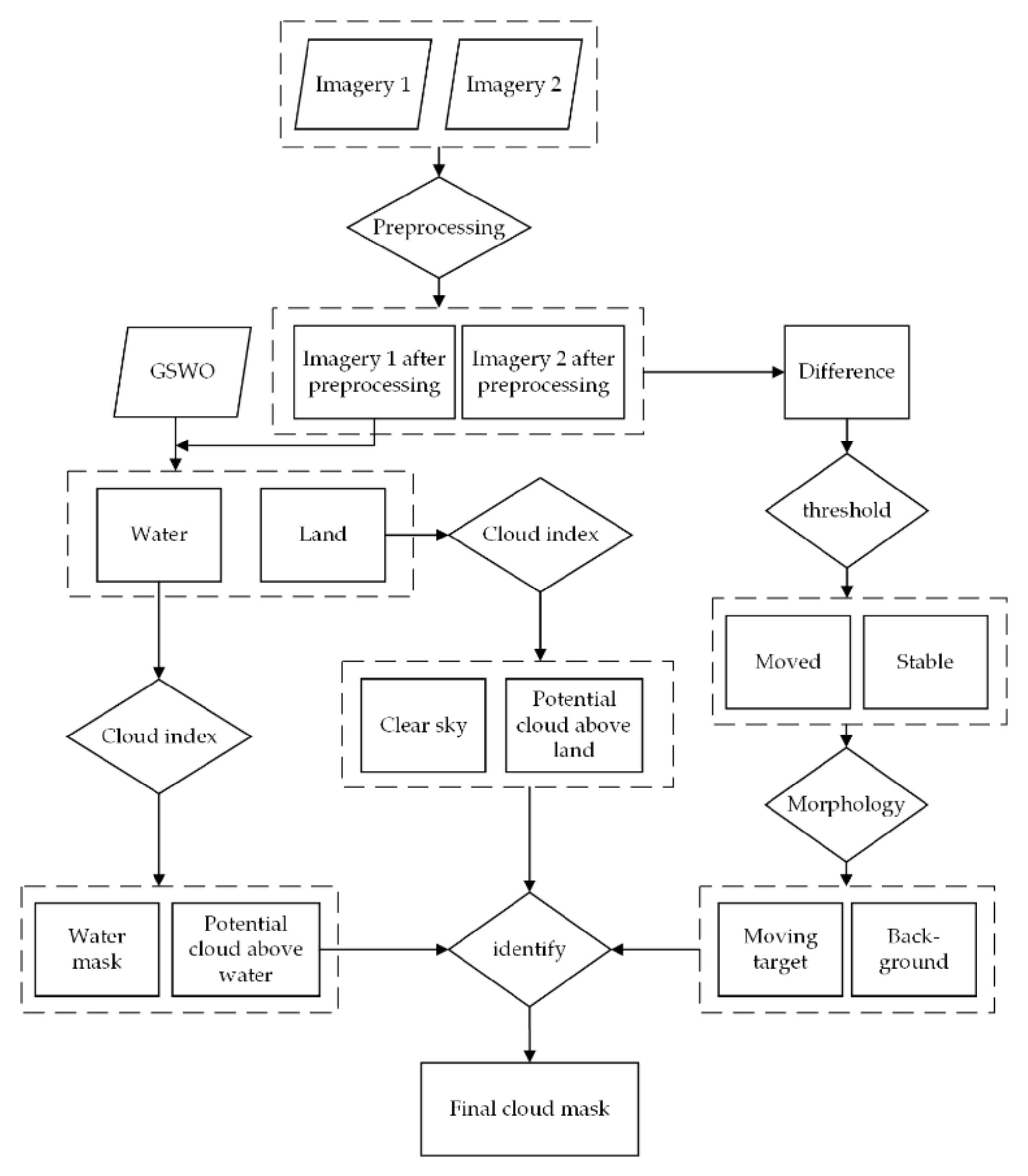
There are four main steps in the RTD method (Figure 2): (1) data preprocessing; (2) computing a series of cloud indexes in the image to highlight potential clouds; (3) calculating the difference between two real-time images and further separating dynamic targets from the stable background; and (4) confirming the real cloud pixels by analyzing the physical and dynamic features of clouds. The four main steps of the RTD method are explained in detail in the following paragraph. In order to examine the effectiveness of this method, we conducted three experiments using GF-4 images of the Hainan, Liaoning, and Xinjiang areas.

3.1. Preprocessing

Preprocessing included the following main steps: radiometric calibration, orthographical correction, and geometric correction.

(1) Radiometric calibration. This is used to obtain the Top of Atmosphere (TOA) reflectance. TOA reflectance is the essential attribute of ground objects, which can avoid the influence of solar radiation intensity and solar altitude angle. Absolute radiometric calibration can be performed by taking the absolute calibration coefficients provided by the China Center for Resources Satellite Data and Application. The equivalent radiation brightness is calculated as follows:

$$\mathrm{Le}=\mathrm{Gain}\cdot \mathrm{DN}+\mathrm{Bias}$$

(1)

where Le is the equivalent radiation brightness at the entrance pupil of the satellite loading channel; its unit is W·m⁻²·sr⁻¹·um⁻¹. Gain and Bias means the gain and offset of the calibration coefficient, respectively. Their unit is W·m⁻²·sr⁻¹·um⁻¹, too. DN is the digital number of a pixel. If we wish to calculate the TOA reflectance, it is necessary to consider the solar irradiance (ESUN) at the outer atmospheric for the GF-4 satellite. However, the China Center For Resources Satellite Data and Application did not provide these data. We then calculated the ESUN using the following equation:

$$ESUN=\frac{{\displaystyle {\int }_{\lambda 1}^{\lambda 2}E(\lambda )S(\lambda )d\lambda }}{{\displaystyle {\int }_{\lambda 1}^{\lambda 2}S(\lambda )d\lambda }}$$

(2)

where E(λ) means the solar spectral radiation energy outside the atmosphere. This is obtained from the solar constant and solar spectral irradiance under zero air mass, which was published in 2016 as a meteorological industry standard of the People’s Republic of China. S(λ) means the spectral response function of the sensor at a certain band, and λ1 and λ2 mean the beginning and ending locations of a certain band spectrum, respectively. After determining the Le and ESUN, we finally calculated the TOA reflectance as follows:

$${\rho }_{\lambda }=\frac{\pi \cdot \mathrm{Le}\cdot d^2}{ESUN\cdot sin(\theta )}$$

(3)

where ${\rho }_{\lambda }$ means the TOA reflectance, $\mathsf{\pi }$ is pi (3.1415926), d means the distance between the Sun and the Earth in astronomical units, and $\theta$ means the solar elevation angle.

(2) Orthographical correction and geometric correction. The GSWO data used in the RTD method are derived from Landsat products. These data are in the UTM-WGS84 projected coordinate system and have been radiometrically and geometrically corrected. The downloaded GF-4 data are a level 1A product and are in the GCS-WGS-1984 geographic coordinate system and have not been radiometrically or geometrically corrected. There will be a huge positional deviation if the Landsat and GF-4 images are directly combined, and accordingly orthographical correction and geometric correction should be performed in advance. Orthographical correction was firstly performed using the rational polynomial coefficient (RPC) model [31]. GF-4 provides the PRC values in its metadata. Geometric correction was performed using Landsat images as reference images. In order to ensure that the correction was accurate, we performed geometric correction three times. Geometric correction was firstly performed between two GF-4 images and the Landsat reference image separately, and then geometric correction was performed again between the two corrected GF-4 images. Thus, we ensured that the geometric corrections had a high matching accuracy. We performed these correction operations using the ENVI 5.3 software and controlled all the RMSEs to less than 2 pixels.

3.2. Potential Cloud Pixels Detection from Single Image

(1)

Separate land and water with GSWO data

As land and water surfaces have very different spectral characteristics, it is essential to determine whether the underlying surface type is land or water before cloud detection can be achieved [11,16,18]. Cloud indexes are commonly calculated separately for land and water surfaces [18]. In previous cloud detection methods, a water mask was obtained through several spectral tests [19]. This approach can separate land and water pixels well when they are clear-sky or thin cloud pixels; however, it does not work for areas covered by thick clouds [16]. It is necessary to develop a water mask that can separate water and land precisely. In recent years, many water products have been developed and used, such as a 30 m water mask from a Landsat-based global land-cover product and a 250 m global water mask from MODIS data [16,18].

GSWO provides water occurrence from 0% to 100% for each pixel [16,30]. A value of 0 means land and a value of 100 means water. The water occurrence is changeable in intertidal zones located near coastlines or terrestrial rivers; however, the value is commonly less than 40%. As such, we can roughly divide the GF-4 images into water and land parts according to Equation (4) as follows:

$$Surface=\left\{\begin{array}{c}Land, \mathrm{if} \mathrm{water} \mathrm{occurrence}\ge 40\% \\ Water, \mathrm{if} \mathrm{water} \mathrm{occurrence} < 40\%\end{array}\right.$$

(4)

It should be noted that this water and land segmentation provides an effective way to guide the subsequent threshold setting. However, GSWO cannot be used to construct an accurate water map for every GF-4 image since the image acquisition time may be different.

(2)

Cloud test

The RTD algorithm combines several spectral tests (as does Fmask) to identify Potential Cloud Pixels (PCPs) [19]. However, only four visible and near-infrared bands were used for GF-4 images. Due to the lack of thermal infrared, cirrus, and short infrared bands, many important spectral parameters cannot be calculated, such as Brightness Temperature (BT), the Normalized Difference Snow Index (NDSI), and the Normalized Difference Built-up Index (NDBI). In the RTD algorithm, six spectral tests of the visible light band were performed.

• Spectral test in a single spectral band

Clouds have high reflectance in the visible light band, so their values are higher than those of ordinary objects. Setting a threshold in the visible band is the simplest way to separate clouds. In our experiment, we firstly used the TOA reflectance of the blue band to separate clouds as follows:

$$Surface=\left\{\begin{array}{c}Cloud, \mathrm{if} \mathrm{band}\_\mathrm{Blue}\ge 0.15 \\ Clear\_sky, \mathrm{if} \mathrm{band}\_\mathrm{Blue} < 0.15\end{array}\right.$$

(5)

The spectral test in a single spectral band can classify most clouds; however, it cannot separate high-reflectance objects, such as sand, rocks, ice, snow, built-up area, etc.

• Whiteness test

The Whiteness Index was originally proposed by [32]. As clouds always appear white due to their flat reflectance in the visible spectrum, these authors used the sum of the absolute difference between the intensity of the visible bands and the overall brightness to calculate the Whiteness Index [19]. Zhu et al. divided this difference by the average value of the intensity of the visible bands and proposed a new Whiteness Index [19]. We examined the index proposed in [19] and found that it works well for distinguishing clouds in GF-4 imagery. As such, we adopted this index in our experiment. It was calculated as follows:

$$Surface=\left\{\begin{array}{c}Cloud, \mathrm{if} \mathrm{Whiteness}\le 0.5 \\ Clear\_sky, \mathrm{if} \mathrm{Whiteness} > 0.5\end{array}\right.$$

(6)

where

$$\mathrm{Whiteness}=\left(\right(\mathrm{band}\_\mathrm{Blue}+\mathrm{band}\_\mathrm{Green}+\mathrm{band}\_\mathrm{Red})-3\cdot MeanVis)/MeanVis$$

(7)

$$MeanVis=(\mathrm{band}\_\mathrm{Blue}+\mathrm{band}\_\mathrm{Green}+\mathrm{band}\_\mathrm{Red})/3$$

(8)

band_Blue, band_Green, and band_Red mean the TOA reflectance in the blue, green, and red channels, respectively. The Whiteness Test can be used to remove those pixels whose spectra are not sufficiently flat relative to cloud. However, neither the original Whiteness Index nor the new Whiteness Index of Zhu et al. can distinguish certain pixels of bare soil, sand, built-up area, and snow/ice, since these are also very bright and have a “flat” reflectance in the visible bands.

• HOT test

The Haze Optimized Transformation (HOT) was firstly developed and assessed for the detection and characterization of the spatial distribution of haze/cloud in Landsat scenes [33]. It is based on the idea that, for most land surfaces under clear-sky conditions, the visible bands are highly correlated but the spectral response to haze and thin cloud is different between the blue and red wavelengths [19]. It is described as

$$\mathrm{HOT}=\mathrm{band}\_\mathrm{Blue}-k\cdot \mathrm{band}\_\mathrm{Red}-b$$

(9)

where k and b are the correlation coefficient and intercept of the TOA reflectance of the blue and red bands, respectively. These were derived from the images in the clear-sky area. However, in real experiments, it is not easy to calculate k and b for every image. Zhu et al. proposed the new format of HOT [19]. It pre-defines several parameters so that it is not necessary to calculate the parameters separately for each image. In this study, we adopted the HOT index proposed in [19], which is described as follows:

$$\mathrm{HOT}=\mathrm{band}\_\mathrm{Blue}-0.5\cdot \mathrm{band}\_\mathrm{Red}$$

(10)

$$Surface=\left\{\begin{array}{c}cloud, \mathrm{if} \mathrm{HOT} \le 0.15\\ Clear\_sky, \mathrm{if} \mathrm{HOT} > 0.15\end{array}\right.$$

(11)

The HOT is useful for detecting clouds, and especially thin clouds; however, it cannot be applied to identify water, snow, or bare soil surfaces due to the irregularity of these surfaces in the red and blue bands.

• NDVI test

The Normalized Difference Vegetation Index (NDVI) can be used to describe the vegetation situation in an image. The NDVI is calculated as follows:

$$\mathrm{NDVI}=(\mathrm{band}\_\mathrm{NIR}-\mathrm{band}\_\mathrm{Red})/(\mathrm{band}\_\mathrm{NIR}+\mathrm{band}\_\mathrm{Red})$$

(12)

where band_NIR and band_Red mean the TOA reflectance of the near-infrared and red channels, respectively. Chlorophyll in vegetation is a strong absorber of red light; however, it strongly reflects in the near-infrared. As such, vegetation presents a high value of NDVI. Meanwhile, clouds present similar reflective features in the red and NIR bands, so their NDVI values fluctuate around 0.

$$Surface=\left\{\begin{array}{c}cloud, \mathrm{if} \mathrm{NDVI} < 0.1\\ Clear\_sky, \mathrm{if} \mathrm{NDVI} \ge 0.1\end{array}\right.$$

(13)

It should be noted that the NDVI test is used to remove the influence of vegetation; however, it cannot be used to remove water, snow, etc., since their NDVI values are also near zero.

• NDWI test

The Normalized Difference Water Index (NDWI) can be used to describe the water situation in an image [34]. The NDWI is calculated as follows:

$$\mathrm{NDWI}=(\mathrm{band}\_\mathrm{Green}-\mathrm{band}\_\mathrm{NIR})/(\mathrm{band}\_\mathrm{Green}+\mathrm{band}\_\mathrm{NIR})$$

(14)

where band_NIR and band_Green mean the TOA reflectance of the near-infrared and green channels, respectively. Water has a strong absorption in the NIR; however, it strongly reflects green light. As such, water commonly presents high values of NDWI. Meanwhile, clouds present similar reflective features in the green and NIR bands, and their NDWI value is commonly lower than 0.3. As such, NDWI test is given by the following equation:

$$Surface=\left\{\begin{array}{c}cloud, \mathrm{if} \mathrm{NDWI} < 0.3\\ Clear\_sky, \mathrm{if} \mathrm{NDWI} \ge 0.3\end{array}\right.$$

(15)

Similar to the NDVI test for vegetation, the NDWI test is only used to remove the influence of water. The clear_sky pixels were probably water to a large extent.

Clouds result in a single image can be finally obtained through the following equation:

$$\begin{array}{l}Cloud=\mathrm{band}\_\mathrm{Blue}\left(\mathrm{true}\right)\cap \mathrm{Whiteness}\left(\mathrm{true}\right)\cap \\ \mathrm{HOT}\left(\mathrm{ture}\right)\cap \mathrm{NDVI}\left(\mathrm{true}\right)\cap \mathrm{NDWI}\left(\mathrm{true}\right)\end{array}$$

(16)

3.3. The Difference between a Pair of Real-Time Images

Clouds are masses of condensed water vapor floating in the atmosphere. They may be in a liquid or solid state and may consist of a mixture of water and ice, and their dynamics, growth, motion, and dissipation are very complex [35]. Clouds are spatial features that evolve over time [36]. Generally, the height of clouds is more than 600 m above the ground surface. The wind speed is more than 20 m/s at such a height. In the stratosphere, the wind speed greatly increases due to the airstream. The time interval between two GF-4 images can reach 20 s. Assume that two images are obtained two minutes apart. In such a time, it is reasonable to assume that changes in the land surface are negligible. However, clouds can move by at least 240 m in this time. The spatial resolution of GF-4 is 50 m pixel. As such, it is theoretically possible to detect the movement of clouds using GF-4 images. In real experiments, geometric correction errors should be considered. Generally, the geometric correction errors can be controlled to within two pixels.

For the purpose of moving target detection, clouds can be regarded as the moving target that should be detected. Moving objects can be identified using the difference between two images if the difference is larger than a given threshold. The moving test can be described as follows:

$$D_k(x,y)=\left|I_{k+1}(x,y)-I_k(x,y)\right|$$

(17)

$$Surface=\left\{\begin{array}{c}cloud, \mathrm{if} D_k(x,y)\ge 0.01\\ background, \mathrm{if} D_k(x,y)<0.01\end{array}\right.$$

(18)

where x and y refer to the row and column number of a pixel, respectively; I_k(x,y) refers to the pixel value of pixel (x,y) at time k; I_k+1(x,y) refers to the pixel value of pixel (x,y) at time k+1; and D_k(x,y) refers to the difference between the two images. The moving test can be used to identify moving clouds by comparing two consecutive images. Due to the images’ coarse resolution, most other moving objects on the Earth cannot be directly detected in GF-4 images, such as buses, trains, and airplanes. Therefore, clouds can be regarded as the only moving targets in GF-4 images. However, there are some problems in real cloud detection experiments. The first one is due to the errors caused by the geometric correction. Second, clouds which overlap in two images can easily be identified as background due to “holes”—i.e., pixels which contain clouds in the first image but which still contain clouds in the second image—produced in the difference process. In order to overcome these two problems, we applied some morphological algorithms, including corrosion, dilation, and flood-fill algorithms [37]. Firstly, a corrosion process was performed to reduce the errors caused by geometric correction and isolated noise caused by system errors. Then, an image segmentation was performed. The eroded images were taken as starting points and the segmentation result was taken as the boundary to use in the flood-fill algorithm. Thus, we obtained a rough cloud result. Dilation was then performed to expand the cloud boundary in order to obtain nearly all of the moved clouds. Finally, the dilated clouds were intersected with the cloud result that was obtained from the cloud index to obtain the final cloud mask.

3.4. Evaluation of RTD by Comparison with SVM

In order to demonstrate the accuracy and effectiveness of the proposed RTD method, this method was compared with the SVM classifier. SVM has been proven to be a highly accurate machine-learning method. Therefore, SVM can be considered as an important benchmark to assess the performance of RTD. A brief description of SVM is presented in the following equation. Assume there are l observations from two classes:

$$\{(x_1,y_1),(x_2,y_2),\dots ,(x_l,y_l)|x_i\in R^N,y_i\in \{-1,1\}\}$$

(19)

where $x_i$ denotes the samples; y_i is a collection of labels that represent the category of $x_i$, and $i$ is the i-th sample. Let us assume that two classes are linearly separable. This means that it is possible to find at least one hyperplane (linear surface), defined by the vector $w\in R^N$ and bias $b\in R$, that can separate the two classes without errors. Finding the optimal hyperplane involves solving a constrained optimization problem using a quadratic equation. The optimization criterion is the width of the margin between the classes. The discrimination hyperplane is defined as follows [38]:

$$f(x)={\displaystyle \sum _{i=1}^l{y}_i{a}_{i}k(x,x_i)+b}$$

(20)

where $k(x,x_i)$ is a kernel function and where the sign of $f(x)$ denotes the membership of $x$. Constructing the optimal hyperplane is equivalent to finding all nonzero $a_i$ values, which are called Lagrange multipliers. Any data point $x_i$ corresponding to a nonzero $a_i$ is a support vector of the optimal hyperplane [39].

In the process of implementing SVM, we used the same reference images as in RTD to obtain the best parameters for the SVM. We tested the linear, polynomial, radial basis, and sigmoid kernel functions, and selected the radial basis kernel function. We then further tested the gamma and penalty parameters. The value of gamma was set to 0.2 and the penalty parameter was set to 100 to classify the cloud.

At the same time, SVM and RTD were compared using the same validation data. We adopted six commonly used indicators to assess the accuracy of the results, namely the overall accuracy (OA), Kappa coefficient, commission error (CE), omission error (OE), producer’s accuracy (PA), and user’s accuracy (UA) [40]. By using the same reference images and validation set, we guaranteed the fairness of the comparison between SVM and RTD.

4. Results

4.1. Hainan Area

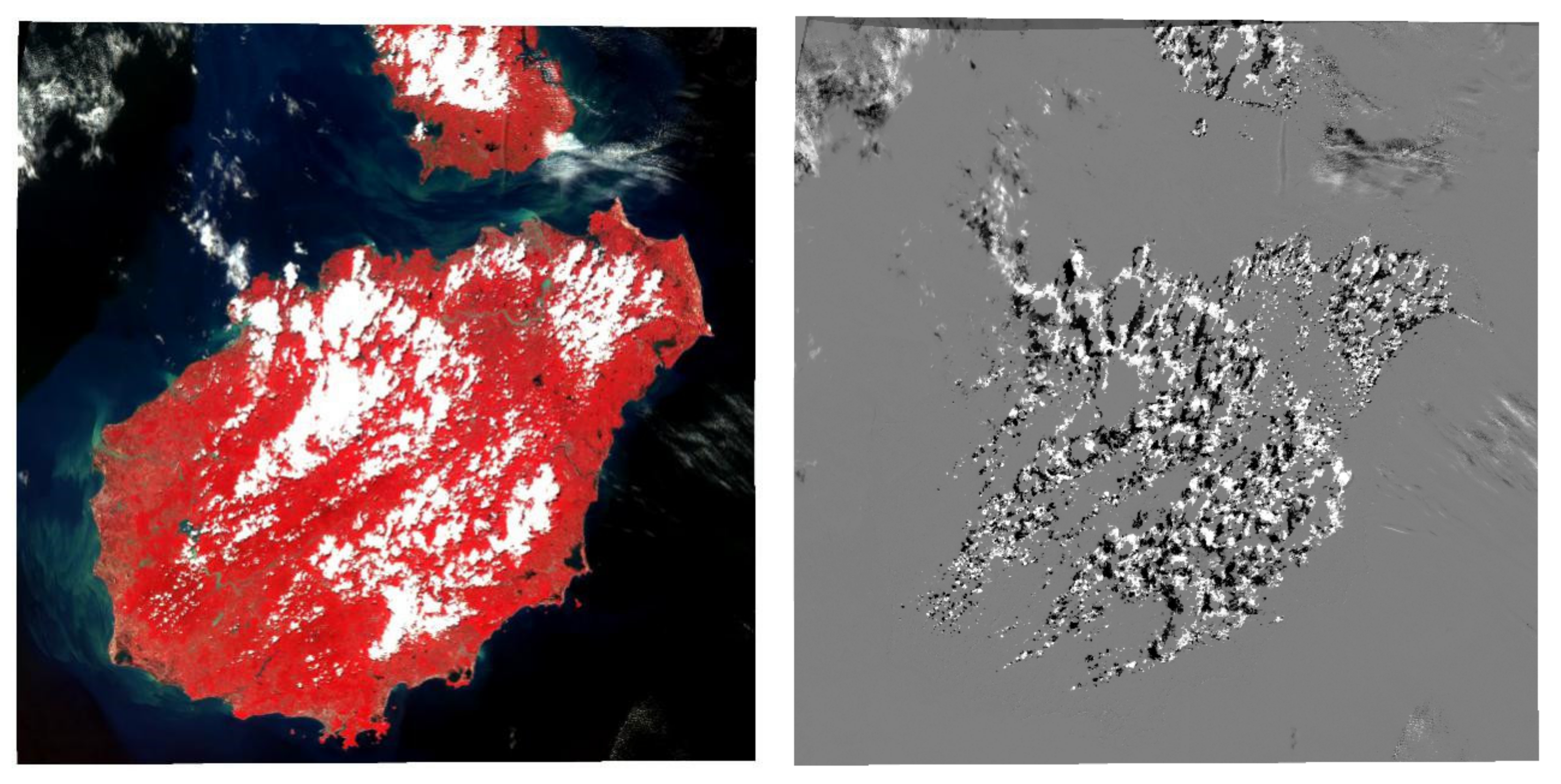
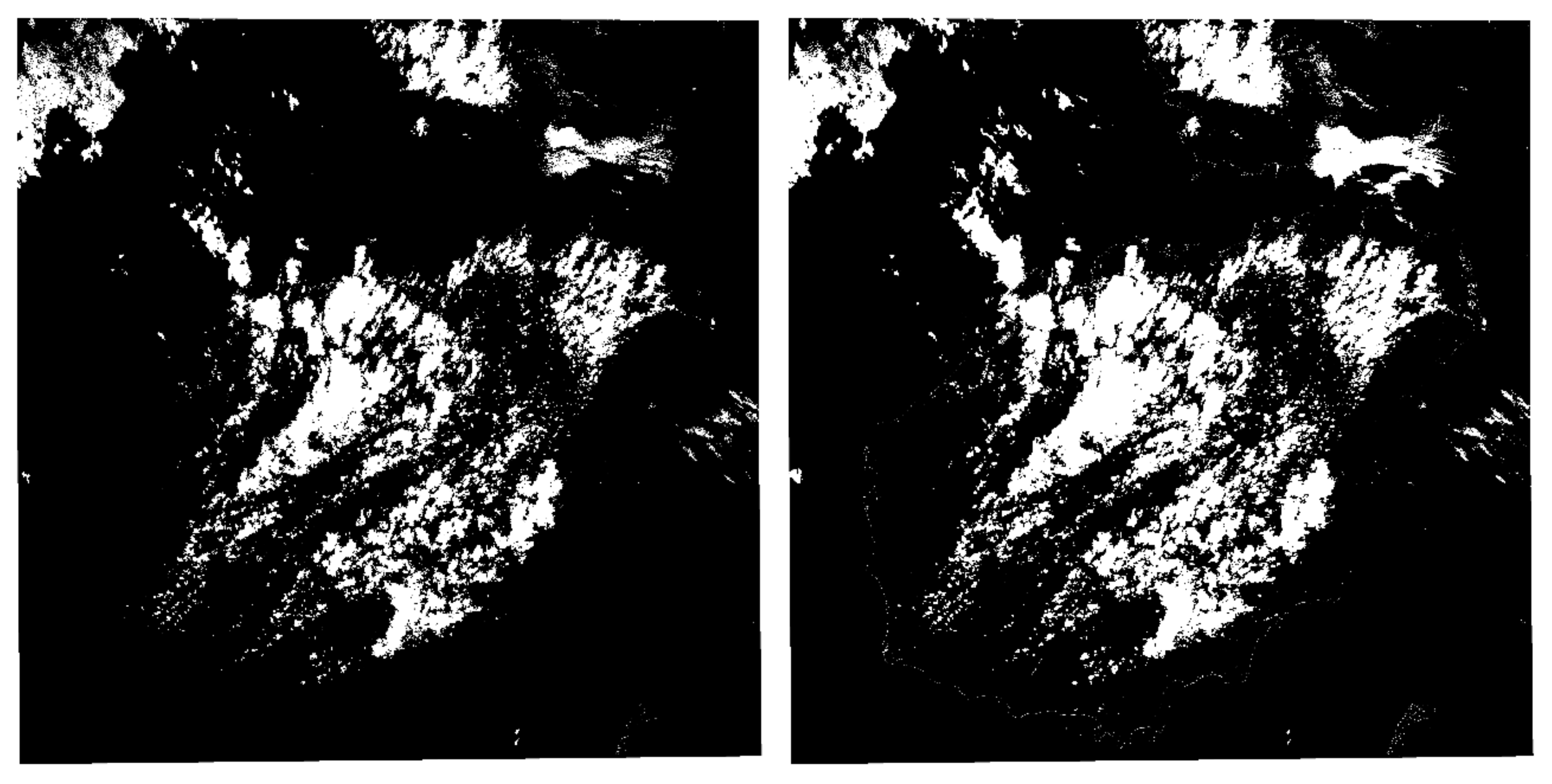
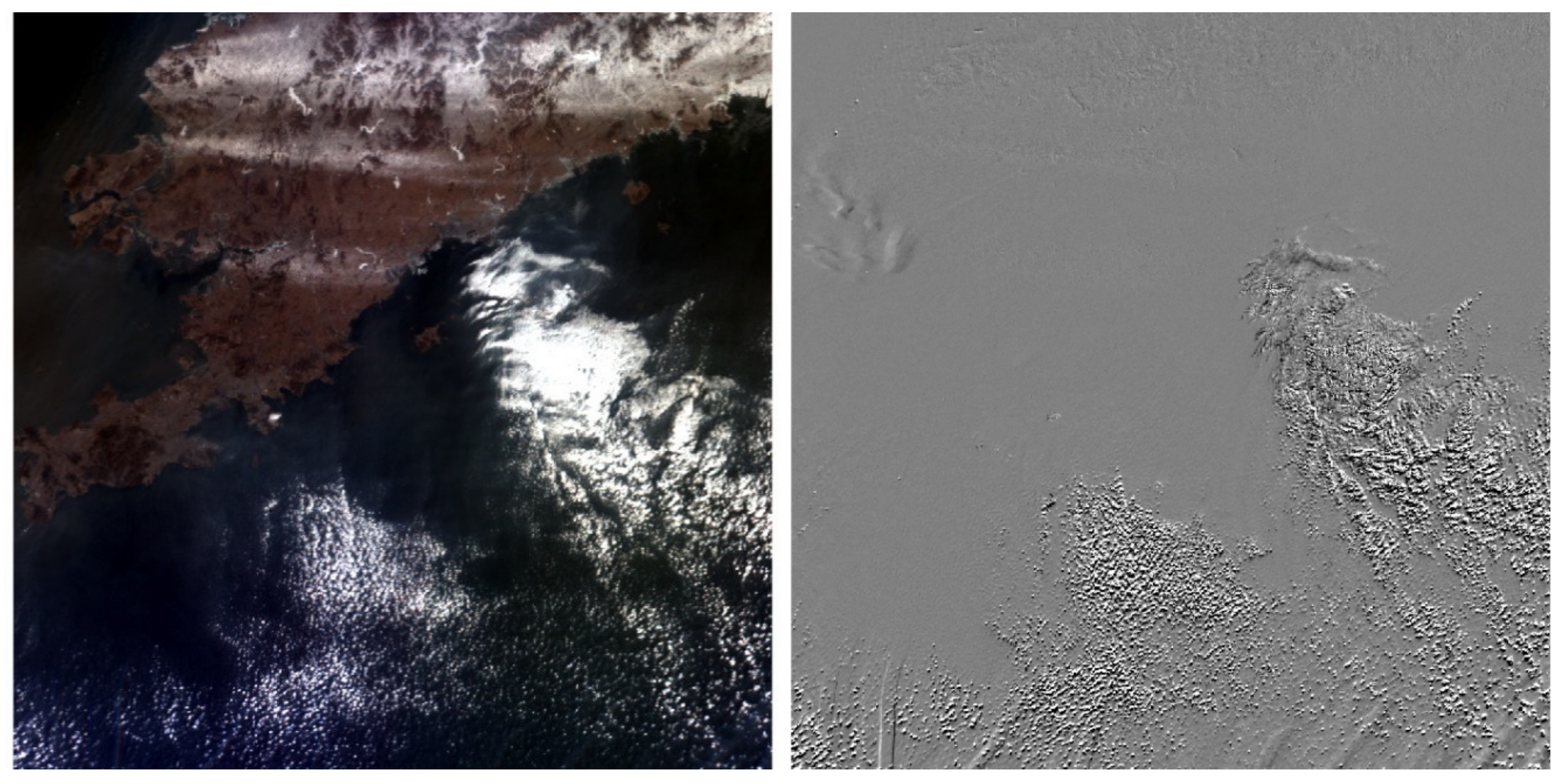
The Hainan area was first used to demonstrate the effect of the cloud detection ability of the RTD method. Hainan has a complex water and land background. The original image and the difference map of time-adjacent images are shown in Figure 3. Additionally, a visual comparison of the results of the RTD and SVM methods is shown in Figure 4. Both methods can identify most clouds and background accurately and showed a comparable cloud detection accuracy. Only some dikes around the coastline and some buildings were wrongly classified as clouds by the SVM method, since they are very bright and have similar spectral features to clouds in the visible and NIR bands.

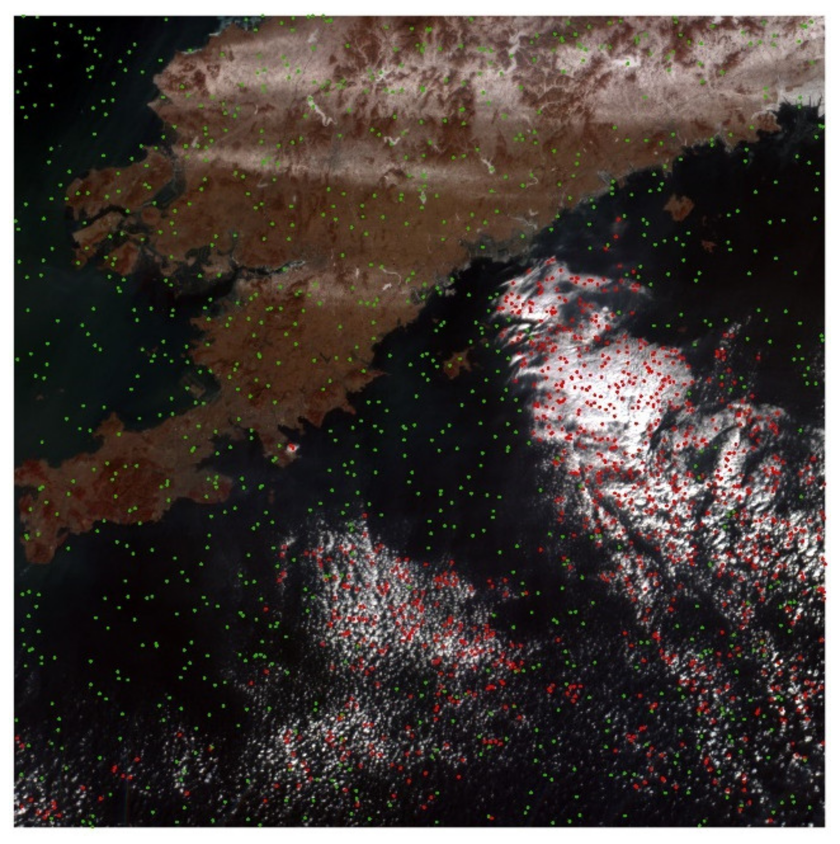
Furthermore, a quantitative accuracy assessment was performed using 2000 random points generated from manual masks (Figure 5). The results are shown in

Table 4. The overall accuracy (OA) and Kappa coefficient of the Support Vector Machine (SVM) and Real-Time-Difference (RTD) methods for the Hainan images.

	OA	Kappa
SVM	95.5%	0.91
RTD	95.9%	0.92

and

Table 5. The cloud commission error (CE), omission error (OE), producer’s accuracy (PA), and user’s accuracy (UA) of the SVM and RTD methods for the Hainan images.

	CE	OE	PA	UA
SVM	5.48%	3.40%	96.60%	94.52%
RTD	1.07 %	7.20%	92.80%	98.93%

. The SVM and RTD methods obtained a comparable OA and their results are very similar. However, in the SVM method, some errors were produced around the coastline, and it is difficult to distinguish many bright objects from clouds. These objects are mainly dikes and the roofs of some buildings. Compared to the SVM method, the RTD method achieved a higher UA but a lower PA. The lower PA of the RTD method can be contributed to the presence of thin and isolated clouds; such clouds have little influence on the DN value, and their difference values are very small. In the RTD method, these clouds were regarded as stable background in the difference process and were therefore wrongly classified. As such, the SVM and RTD methods achieved similar overall accuracies.

4.2. Liaoning Area

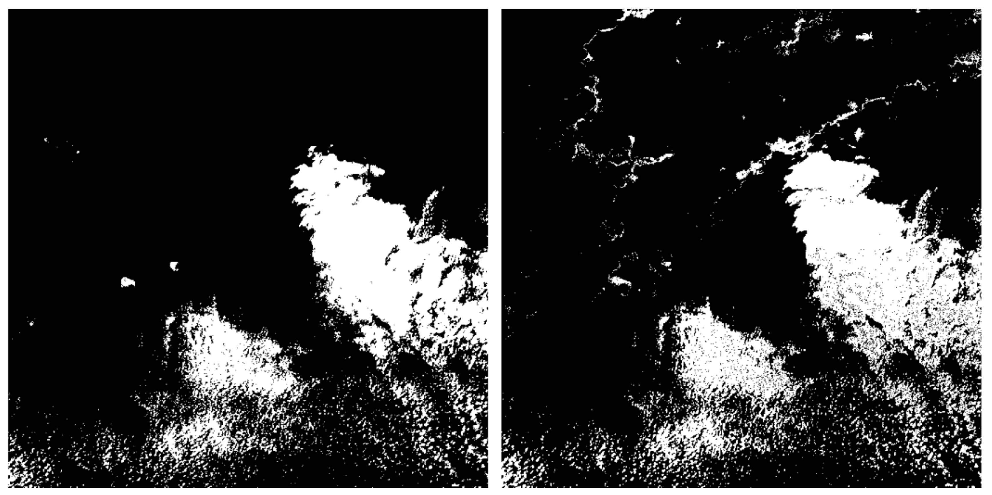
We adopted a similar strategy for the Liaoning area. The situation of the Liaoning area is slightly more complex than the Hainan area since there are some frozen lakes and coastline in this area. The original image and difference map of the time-adjacent images are shown in Figure 6. A visual comparison of the results of the RTD and SVM methods is shown in Figure 7. From this figure, it can be seen that the RTD method showed a strong ability to distinguish ice and bare soil from cloud. However, SVM had difficulty in distinguishing most ice and bare land from clouds, misidentifying many frozen rivers as clouds, and had great difficulty in accurately distinguishing between ice, bare soil, and clouds. The reason for this may be that ice and bare soil are very bright and have very similar spectral features to clouds in the visible and NIR bands.

Quantitative accuracy assessments were obtained using 2000 random points generated from the manual masks (Figure 8). The numerical results are shown in

Table 6. OA and Kappa coefficient of the SVM and RTD methods for the images from the Liaoning area.

	OA	Kappa
SVM	91.15%	0.82
RTD	94.10	0.88

and

Table 7. The cloud CE, OE, PA, and UA for the SVM and RTD methods for the Liaoning area.

	CE	OE	PA	UA
SVM	7.71%	10.20%	89.80%	92.29%
RTD	2.99%	9.00%	91.00%	97.01%

. SVM and RTD achieved comparable accuracy; however, RTD performed slightly better. The OA of RTD was 94.1% and that of SVM was 91.15%. The Kappa coefficient of RTD was 0.88 and that of SVM was 0.82. RTD achieved a lower CE and OE and a higher PA and UA. The results show that RTD can more accurately identify clouds than SVM.

4.3. Xinjiang Area

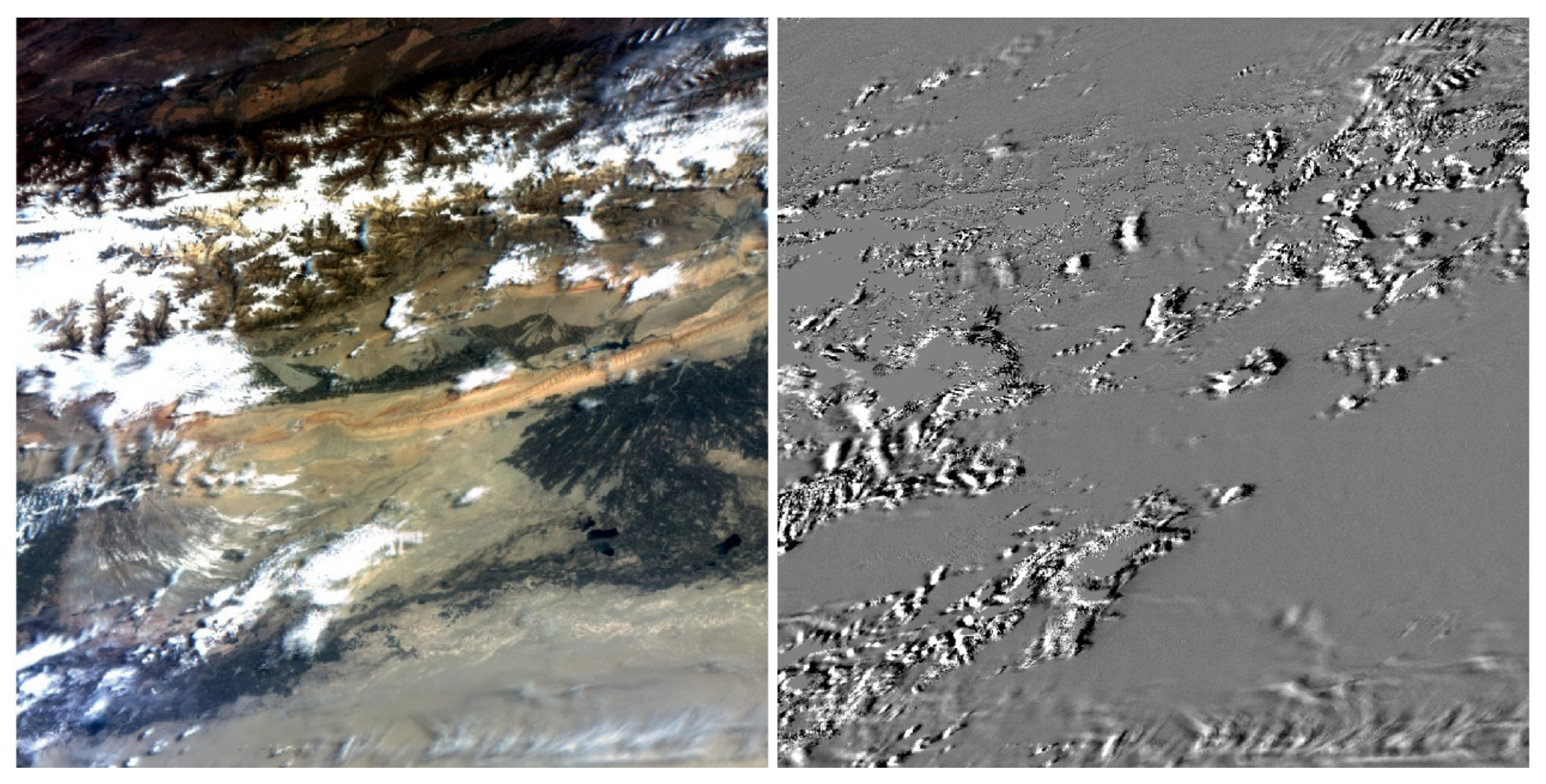
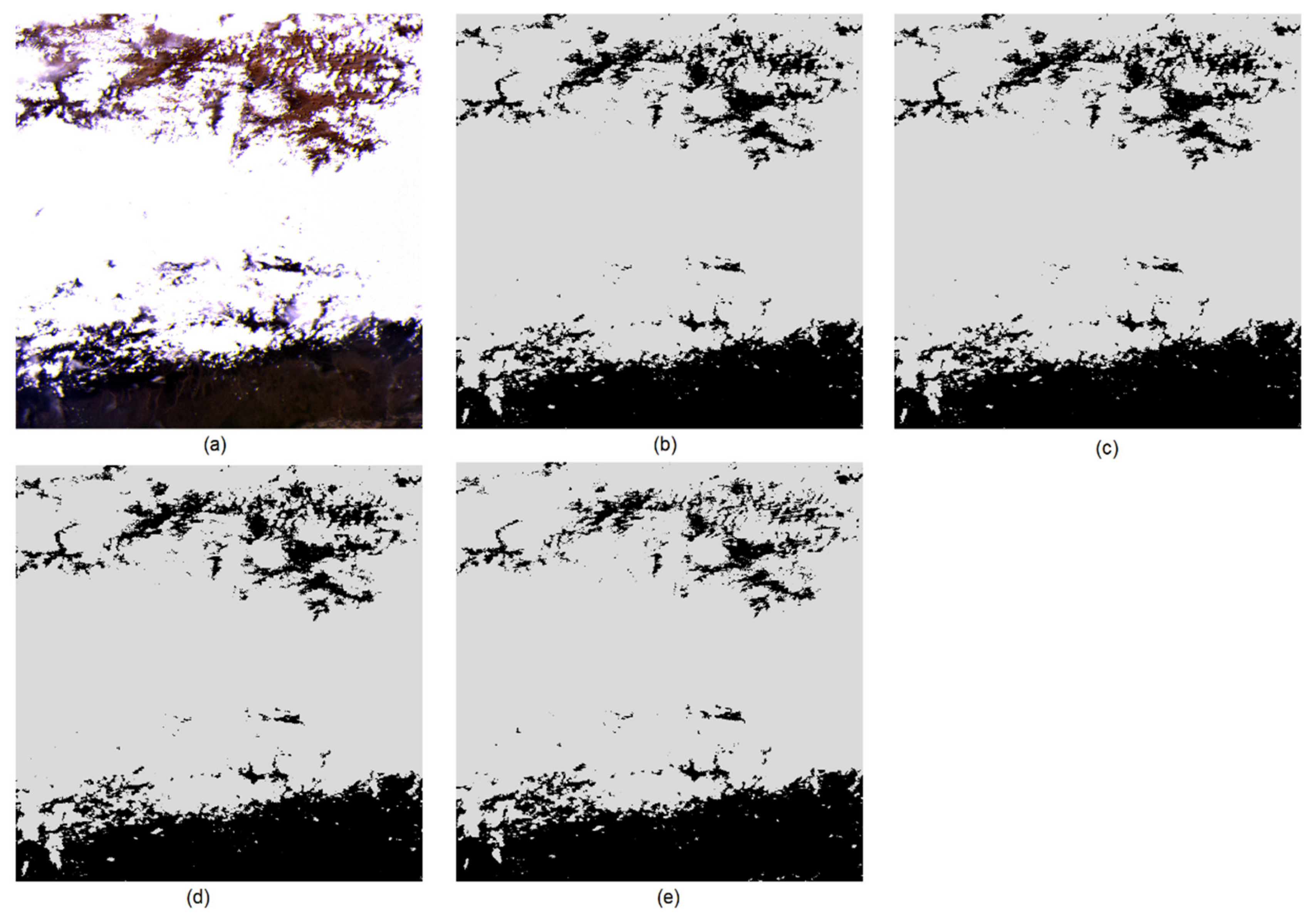
In order to further demonstrate the effectiveness of RTD in cloud detection, we present another experiment in the Xinjiang area. In this area, there are numerous mountains whose tops are covered by large amounts of ice and snow, which complicates cloud detection. As before, we used the RTD and SVM methods to classify the clouds in this area. The original image and the real-time difference image are shown in Figure 9, and the final results obtained by the RTD and SVM methods are shown in Figure 10.

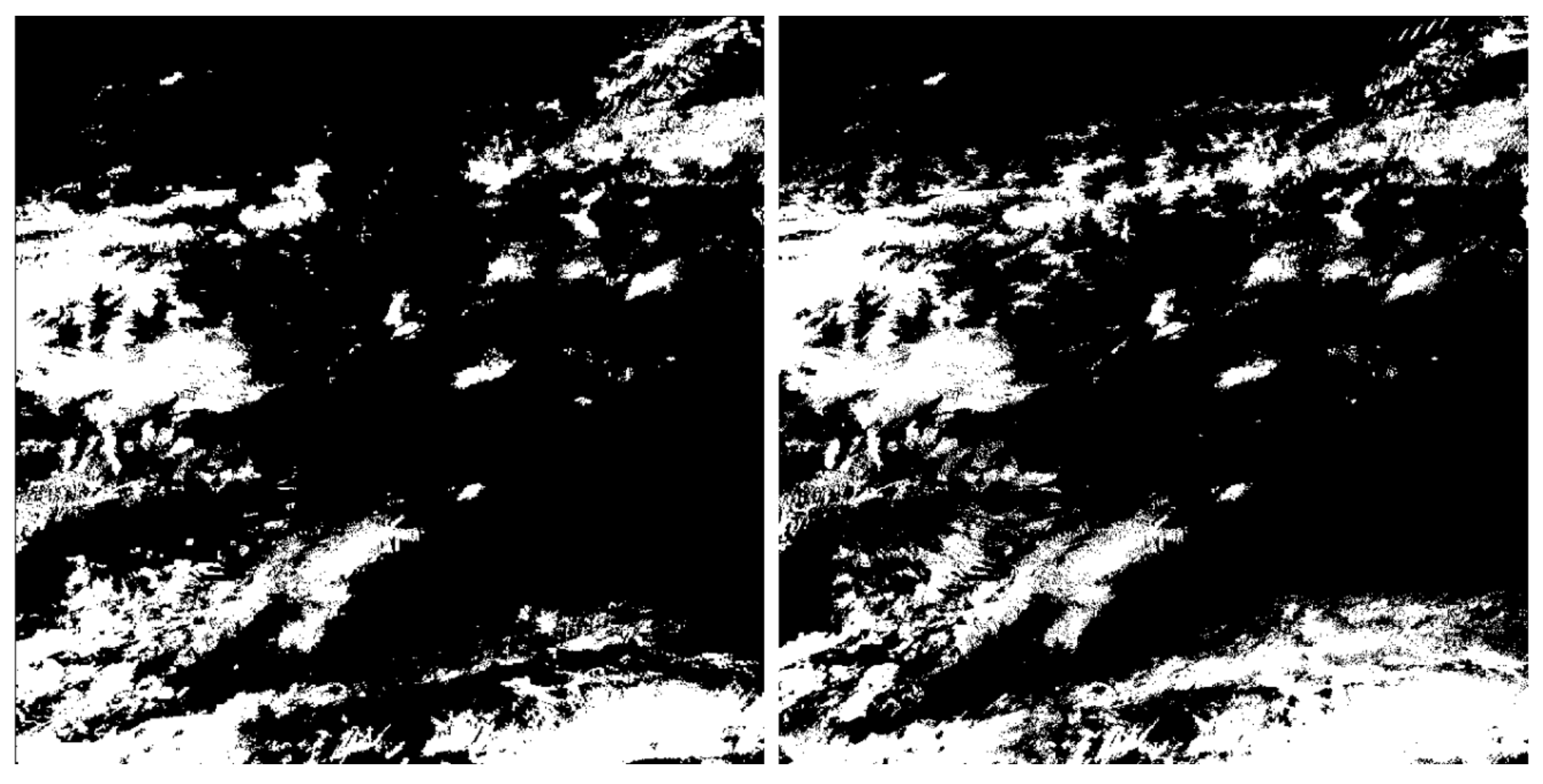
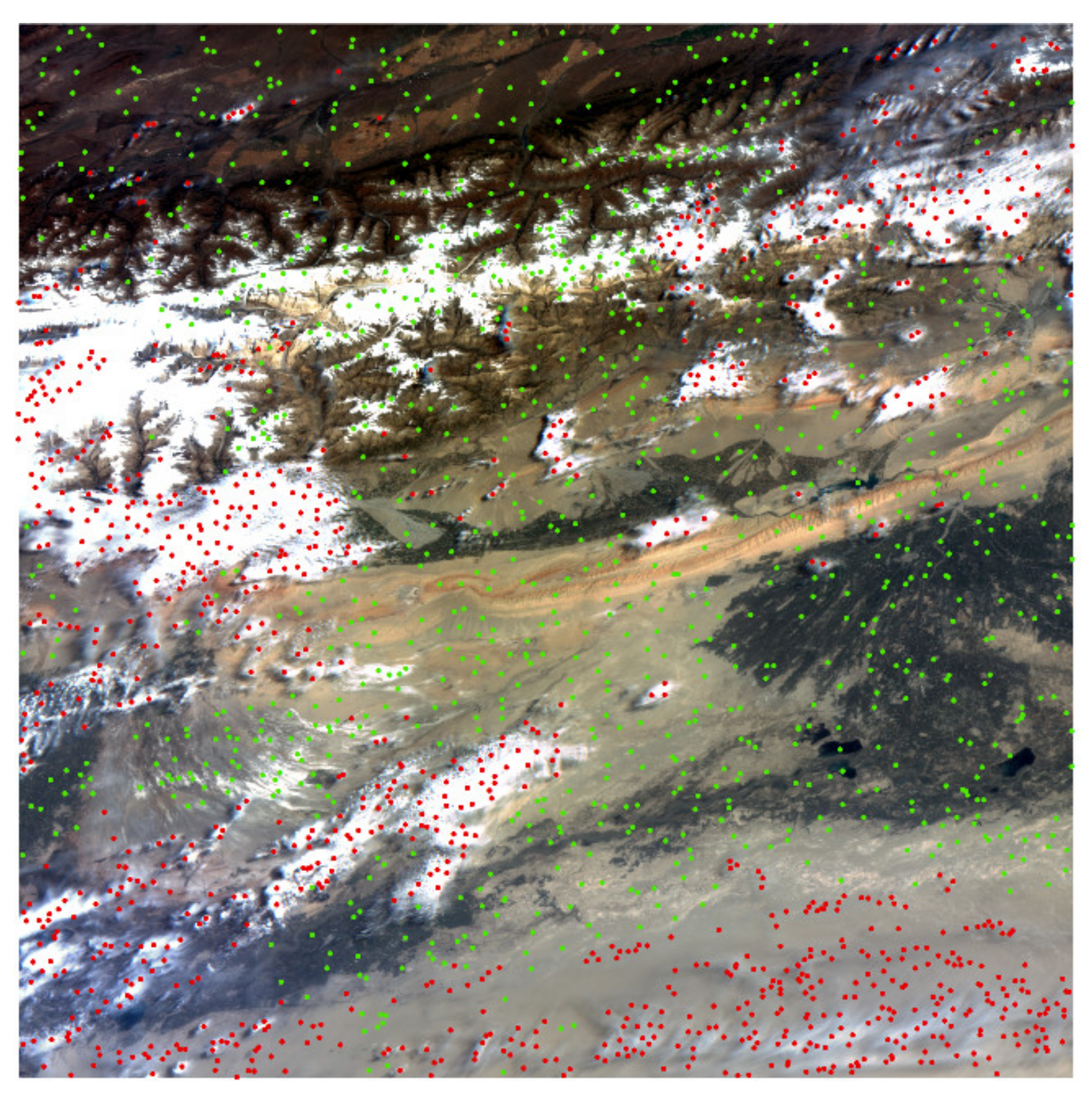
We can see that snowy mountains are very challenging to separate from clouds. The SVM method classified nearly all the snowy mountains as cloud. However, in the RTD method, some of the mountains were deleted. Therefore, in the RTD method, when some clouds are above mountains they will be regarded as moved cloud. However, the RTD method did not remove all the snowy mountains. Quantitative accuracy assessments were also performed using 2000 random points generated from the manual masks (Figure 11). The numerical results are shown in

Table 8. OA and Kappa coefficient of the SVM and RTD methods for the images from the Xinjiang area.

	OA	Kappa
SVM	89.2%	0.784
RTD	93.9%	0.878

and

Table 9. The cloud CE, OE, PA, and UA for the SVM and RTD methods for the Xinjiang area.

	CE	OE	PA	UA
SVM	15.43%	4.1%	95.9%	84.57%
RTD	4.55%	7.8%	92.2%	95.45

. As shown in the tables, the RTD method achieved a higher OA and a higher Kappa coefficient. The SVM method obtained a higher PA but a much lower UA. As such, the SVM method had a lower OA. Conversely, the RTD method had a lower PA but a much higher UA. In the spectral test process of the RTD method, nearly all the cloud pixels were captured. This is very similar to SVM, as can be seen in Figure 12. However, when the RTD process was performed, some thin, small, and isolated clouds were deleted, which caused a slight decrease in the PA. However, this process was beneficial overall since it removed more snowy mountains and improved the OA.

5. Discussion

5.1. Advantages and Disadvantages of the RTD Method

Cloud detection is a necessary step for many applications of optical satellite images before further processing [18]. Many methods have been proposed to screen clouds in optical images. However, these methods may not perform well in terms of distinguishing clouds from ice and snow. This study proposed an algorithm named RTD in an attempt to produce an accurate cloud mask for GF-4 imagery. The RTD algorithm was tested using GF-4 images from three sites with different backgrounds. An excellent classifier, namely SVM, was used to evaluate the performance of RTD. The results show that RTD can obtain accurate cloud masks in the studied images. The good performance of RTD can be attributed to the following aspects:

First, RTD takes full advantage of the real-time imaging features of geostationary satellites. The most important feature of geostationary satellites is that they allow the nearly continuous collection of visible and NIR images of the Earth [41]. Additionally, the revisiting period can reach 20 s for the same region, which is impossible for elliptical satellites. Therefore, it is possible to detect the movement of clouds in real-time using time-adjacent images from a geostationary satellite. Accordingly, in this study, we selected a pair of time-adjacent images to extract the clouds, whose time interval is about 2 or 3 min. As the time interval between images is short, the cloud shapes changed little, and it was consequently very easy to obtain the boundary of moved clouds. If the time interval is too long, it is very challenging to observe the movement of clouds since the shape of clouds continuously changes [42]. Thus, RTD provides a very suitable way to detect clouds using images from geostationary orbit satellites. This is the most important advantage of the RTD algorithm. Another advantage of RTD is that it can identify clouds effectively even without using thermal or cirrus bands. Although ice and snow have similar spectra to clouds in the visible and near-infrared bands, they are usually stationary in the spatial domain. They can be erased as background in difference processes. This advantage makes RTD easy to use with images from most sensors of geostationary satellites. The RTD algorithm provides a more practical way to overcome the difficulties in using GF-4 imagery to monitor clouds. These two advantages ensure that the RTD can obtain more accurate cloud masks. We present the result of an intermediate process of RTD to demonstrate how the RTD improves the cloud-detection accuracy.

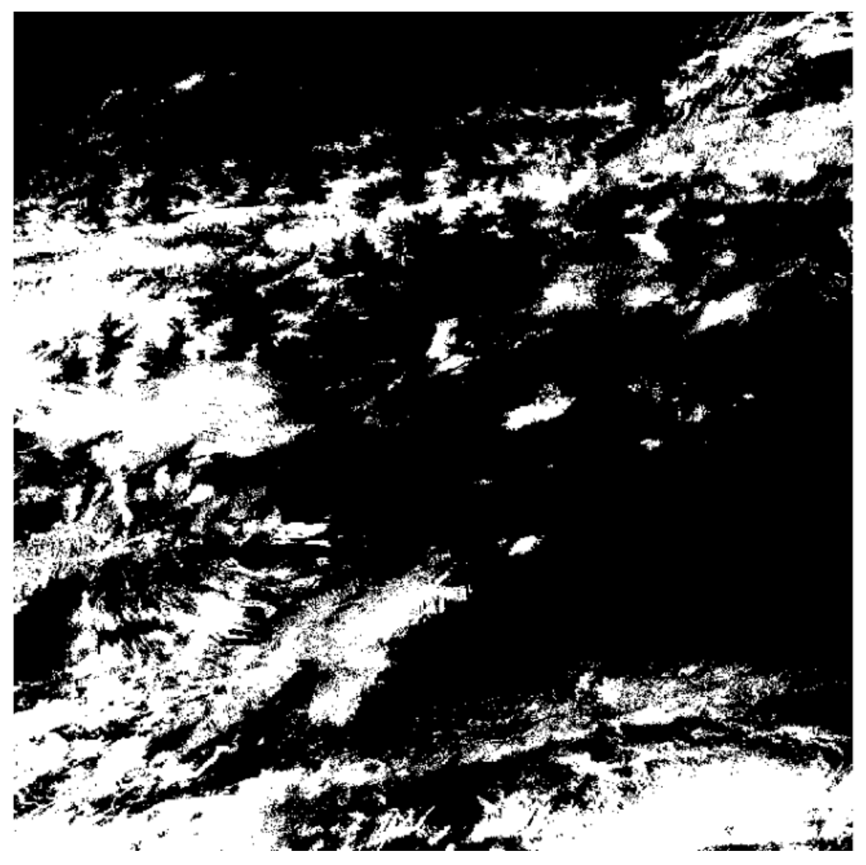
The results of the spectral test of the RTD method in Xinjiang were shown in Figure 12. From Figure 10 and Figure 12, we can see that the spectral test of the RTD method achieved comparable results to the SVM method. Additionally, from Table 8, Table 9 and

Table 10. The cloud OA, Kappa, CE, OE, PA, and UA of the spectral test of the RTD in Xinjiang.

OA	Kappa	CE	OE	PA	UA
88.4%	0.768	16.1%	4.9%	95.1%	83.9%

, we further validate that the OA, Kappa, CE, OE, PA, and UA values of the SVM method are very similar to the values obtained from the spectral test. After adding the movement features, RTD obviously improved the UA; however, with the trade-off of a small decrease in the PA. In this way, RTD achieved a better overall accuracy than SVM and the spectral test.

However, there are some limitations to RTD. The biggest disadvantage of this method is that it requires a very precise geometric correction result. RTD is a temporal cloud detection method. In the RTD method, it is of key importance to perform image registration before performing image difference. It is very easy to control the image registration error within two pixels by manually selecting ground control points (GCPs). However, it is still challenging for the automatic selection of GCPs. Another defect is that some thin, small, and isolated clouds are easily missed due to their smaller difference value and area, which reduced the producer’s accuracy of the RTD method.

5.2. Description of the Thresholds Used in This Paper

(1)

The thresholds used in RTD

The DN value of pure cloud pixels is very similar. It is possible to separate them via a fixed threshold. However, the ground surface under clouds has very variable values. This will greatly influence the value of clouds, especially thin clouds. The value of clouds above sand or ice is higher than that above water. As such, a fixed threshold will lead to some errors in separating clouds. We have performed some experiments on several surface types.

Table 11. The cloud detection thresholds for different surface types.

	Sand	Mountain	Vegetation	Ocean	Haze
TOA_Blue	0.3	0.25	0.25	0.15	0.15
NDVI	0.1	0.1	0.3	0.1	0.3
NDWI	0.3	0.1	0.1	0.25	0.3
Whiteness	0.5	0.5	0.5	0.7	0.5
HOT	0.15	0.15	0.15	0.08	0.1

presents the possible thresholds that can be used for these surface types and can help to separate most clouds. These thresholds were determined based on our trial-and-error test.

When calculating the difference between a pair of real-time images, we adopted 0.01 as the threshold. The theoretical value of TOA is between 0 and 1; however, the real value is commonly very low. For example, clouds are very bright; however, a value of 0.15 was used to label these in the blue band. The value of other surface objects is lower than 0.15. In general, the pixel values of adjacent similar objects differ very little, and therefore their TOA value difference value is very near 0. Based on the results of the trial-and-error test, 0.01 was chosen as the suitable value. Under this threshold, these obvious changes can be easily found; however, this threshold is not sensitive to those slight changes.

(2)

Thresholds used in SVM

In order to guarantee the best performance of SVM, we conducted a series of experiments on the selection of various parameters of SVM. When using the SVM classifier, one should first select a kernel function, which gives the weights of nearby data points in estimating target classes. There are four types of kernel function that are commonly used in SVM; these are linear, polynomial, radial basis, and sigmoid. The linear, polynomial, radial basis, and sigmoid functions can be mathematically expressed by Equations (21)–(24), respectively:

$$K\left(x_i,x_j\right)=x_i{}^T{x}_j$$

(21)

$$K\left(x_i,x_j\right)={(g{x}_i{}^T{x}_j+r)}^d, g>0$$

(22)

$$K\left(x_i,x_j\right)=exp\left(-g\Vert x_i-x_j\Vert {}^2\right), g>0$$

(23)

$$K\left(x_i,x_j\right)=tanh\left(g{x}_i{}^T{x}_j+r\right), g>0$$

(24)

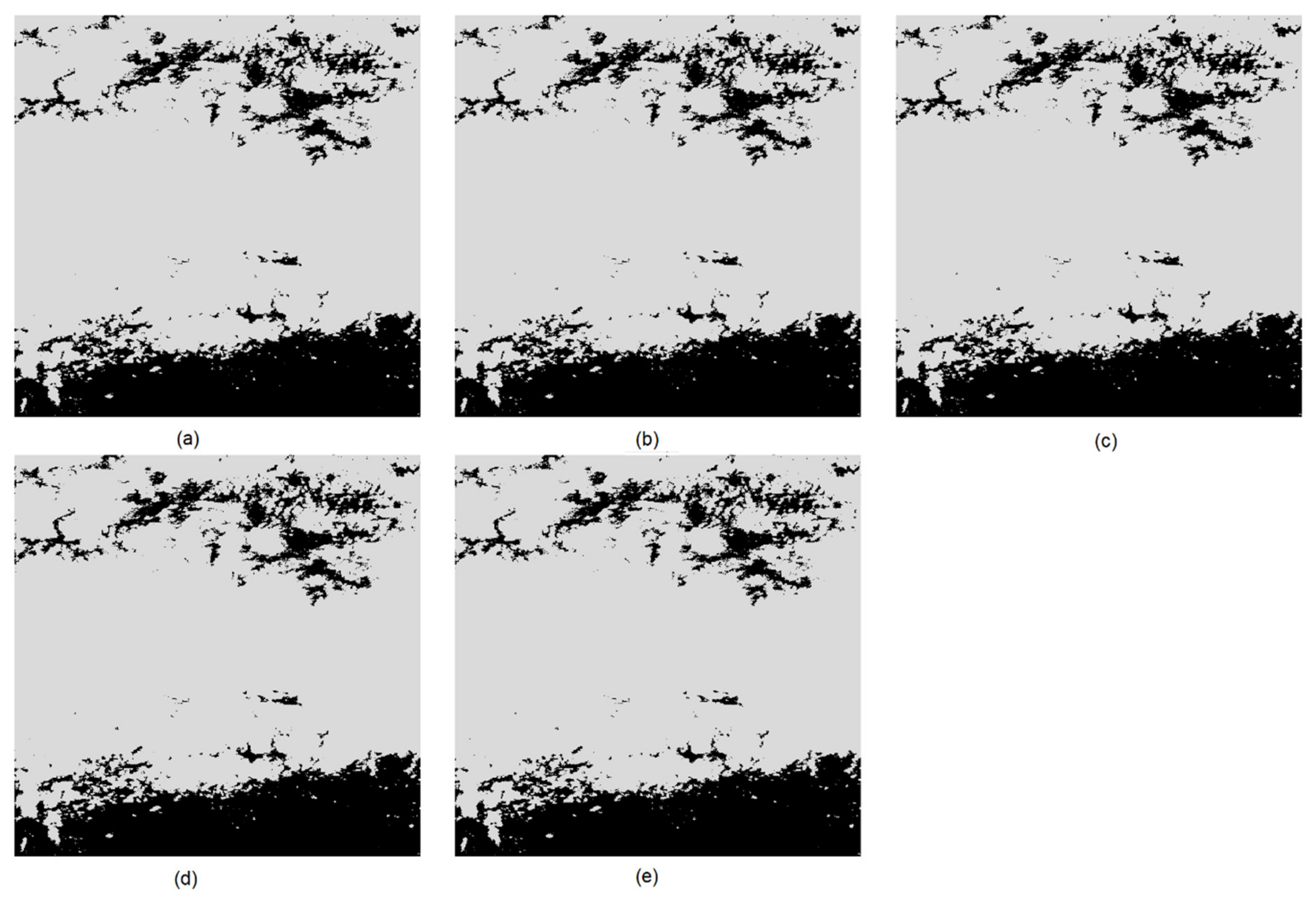
where $g$ is the gamma term in the kernel function for all kernel functions except for linear; d is the polynomial degree term in the kernel function for the polynomial kernel function; and r is the bias term for the polynomial and sigmoid kernel functions. After a trial-and-error test, it was found that the difference between the results of the four kernel functions is very small. A set of cloud detection results are presented in Figure 13. The value of gamma is commonly the inverse of the number of computed attributes, so this value ranges from 0 to 1. The penalty parameter allows a certain degree of misclassification, which is particularly important for non-separable training sets. We tested penalty parameters of 20, 40, 60, 80, and 100 and the results were shown in Figure 14. We found that the difference caused by the selection of kernel function and parameters is very small (commonly less than 0.05%), which is much smaller than the difference between SVM and RTD (nearly 5%). Therefore, this difference will not affect the fairness of the accuracy comparison with RTD.

5.3. MIR Band of GF-4 Images

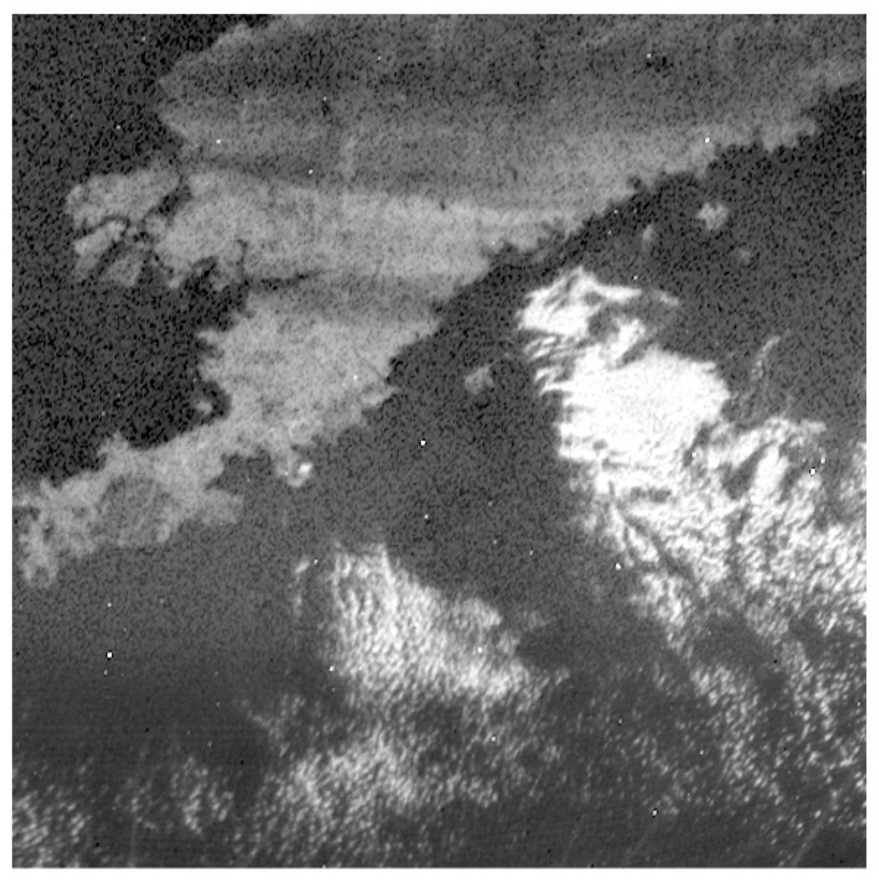
Ice, snow, and bare land present a barrier to cloud identification. Most current cloud detection algorithms rely heavily on thermal and cirrus bands. It is almost impossible to distinguish ice from clouds using optical imagery. In GF-4 imagery, there is an MIR band centered at 3.9 μm, which is a good atmospheric window for cloud detection, being a perfect way to distinguish ice and snow from clouds in single images; in the MIR band, cloud appears bright while ice and snow appear dark due to their low temperature (see Figure 15). However, severe geometric deviations and their coarse resolution make it very hard to match the MIR images with visual and near-infrared images. As mentioned above, it is very difficult to implement automatic image registration between the visual bands and MIR bands. The spatial resolution of the visual and MIR images is completely different. The resampling of MIR imagery causes a large amount of noise in the DN value and makes it difficult to automatically select feature points. We have tested several registration algorithms—such as gray gradient, scale-invariant feature transform (SIFT) [43], speeded up robust features (SRUF) [44], oriented FAST, and rotated BRIEF (ORB) [45]—and found that they were not able to obtain ideal image registration results. It is necessary to choose feature points using artificial puncture points. The coarse resolution of the MIR images makes the process of puncturing points between the MIR images and visual NIR images very challenging and the image registration accuracy very low. Another reason that the MIR band is not used in RTD is that the exposure time of the MIR imagery is slightly shorter (about 45 s) than that of the visual bands; this causes a slight dislocation between the MIR and visible images. Unlike the difference-image technique to detect cloud boundaries, which was described in Section 3.3, dislocation will cause cloud edges to be wrongly identified in visual imagery. This is another reason why MIR was not used in this study. Although there are some OEs, RTD still obtained a satisfactory cloud detection accuracy. Nevertheless, it is possible that the MIR band could be used in future versions of RTD. Additionally, we are working to achieve automatic image registration and fusion between images with different spatial and spectral resolutions.

5.4. Prospects

RTD provides a very convenient and accurate method for cloud detection using images from geostationary orbit satellites. It is particularly useful when using images without thermal infrared and cirrus bands. Affected by the rotation of the Earth and the wind, clouds are constantly in motion. Other high-speed moving objects on the Earth, such as trains, buses, and airplanes, cannot easily be identified in GF-4 imagery due to their small size. Therefore, clouds can be reasonably regarded as the only moving objects that can be detected in GF-4 images. Due to these advantages, we expect RTD to be developed into a new method for the detection of clouds in images from geostationary orbit satellites. However, in order to achieve this goal, it is first necessary to incorporate automatic image registration and a fusion technique, which is key to allowing RTD to achieve automatic cloud detection. On the other hand, more existing remote sensing products, such as land cover, can be used in future experiments.

6. Conclusions

In this study, we developed a novel method, called RTD, to screen clouds in GF-4 imagery, providing a new perspective for cloud detection. This method was tested on three GF-4 images with complicated backgrounds acquired in the Hainan, Liaoning, and Xinjiang areas of China. An excellent classifier, namely SVM, was used for comparison to evaluate the performance of RTD. The results showed that, in the Hainan area, which has large areas of water and land background, RTD and SVM achieved comparable accuracy. However, in the Liaoning and Xinjiang areas, which have large amounts of ice and snow, RTD performed better than SVM. The RTD method combines the spectral features of a single image with the moving features of image time series and improves the cloud detection accuracy compared to traditional methods. We expect that RTD can be developed into a means for the recognition of clouds in images from geostationary orbit satellites.

References

- Yang, A.; Zhong, B.; Wu, S.; Liu, Q. Radiometric cross-calibration of GF-4 in multispectral bands. Remote Sens. 2017, 9, 232. [Google Scholar] [CrossRef] [Green Version]
- Li, F.; Xin, L.; Guo, Y.; Gao, D.; Kong, X.; Jia, X. Super-resolution for GaoFen-4 remote sensing images. IEEE Geosci. Remote Sens. Lett. 2017, 15, 28–32. [Google Scholar] [CrossRef]
- Liu, Y.; Yao, L.; Xiong, W.; Jing, T.; Zhou, Z. Ship target tracking based on a low-resolution optical satellite in geostationary orbit. Int. J. Remote Sens. 2018, 39, 2991–3009. [Google Scholar] [CrossRef]
- Li, P.; Sun, K.; Li, D.; Sui, H.; Zhang, Y. An emergency georeferencing framework for GF-4 imagery based on GCP prediction and dynamic RPC refinement. Remote Sens. 2017, 9, 1053. [Google Scholar] [CrossRef] [Green Version]
- Zhang, Z.; Shao, Y.; Tian, W.; Wei, Q.; Zhang, Y.; Zhang, Q. Application Potential of GF-4 Images for Dynamic Ship Monitoring. IEEE Geosci. Remote Sens. Lett. 2017, 14, 911–915. [Google Scholar] [CrossRef]
- Chen, Y.; Sun, K.; Li, D.; Bai, T.; Huang, C. Radiometric cross-calibration of gf-4 pms sensor based on assimilation of landsat-8 oli images. Remote Sens. 2017, 9, 811. [Google Scholar] [CrossRef] [Green Version]
- Yao, L.; Liu, Y.; He, Y. A novel ship-tracking method for GF-4 satellite sequential images. Sensors 2018, 18, 2007. [Google Scholar] [CrossRef] [PubMed] [Green Version]
- Wu, W.; Liu, W. Remote sensing recognition of residential areas based on GF-4 satellite image. In Proceedings of the 2018 Fifth International Worksho on Earth Observation and Remote Sensing Applications (EORSA), Xi’an, China, 18–20 June 2018; pp. 1–4. [Google Scholar]
- Ju, J.; Roy, D.P. The availability of cloud-free Landsat ETM+ data over the conterminous United States and globally. Remote Sens. Environ. 2008, 112, 1196–1211. [Google Scholar] [CrossRef]
- Lu, Y.; Coops, N.C.; Hermosilla, T. Estimating urban vegetation fraction across 25 cities in pan-Pacific using Landsat time series data. ISPRS J. Photogramm. Remote Sens. 2017, 126, 11–23. [Google Scholar] [CrossRef]
- Zhu, Z.; Woodcock, C.E. Automated cloud, cloud shadow, and snow detection in multitemporal Landsat data: An algorithm designed specifically for monitoring land cover change. Remote Sens. Environ. 2014, 152, 217–234. [Google Scholar] [CrossRef]
- Zhu, Z. Change detection using landsat time series: A review of frequencies, preprocessing, algorithms, and applications. ISPRS J. Photogramm. Remote Sens. 2017, 130, 370–384. [Google Scholar] [CrossRef]
- Chen, B.; Huang, B.; Xu, B. Multi-source remotely sensed data fusion for improving land cover classification. ISPRS J. Photogramm. Remote Sens. 2017, 124, 27–39. [Google Scholar] [CrossRef]
- Shao, Z.; Pan, Y.; Diao, C.; Cai, J. Cloud Detection in Remote Sensing Images Based on Multiscale Features-Convolutional Neural Network. IEEE Trans. Geosci. Remote Sens. 2019, 57, 4062–4076. [Google Scholar] [CrossRef]
- Derrien, M.; Farki, B.; Harang, L.; LeGleau, H.; Noyalet, A.; Pochic, D.; Sairouni, A. Automatic cloud detection applied to NOAA-11/AVHRR imagery. Remote Sens. Environ. 1993, 46, 246–267. [Google Scholar] [CrossRef]
- Qiu, S.; Zhu, Z.; He, B. Fmask 4.0: Improved cloud and cloud shadow detection in Landsats 4–8 and Sentinel-2 imagery. Remote Sens. Environ. 2019, 231, 111205. [Google Scholar] [CrossRef]
- Zhu, Z.; Qiu, S.; He, B.; Deng, C. Cloud and cloud shadow detection for Landsat images: The fundamental basis for analyzing Landsat time series. In Remote Sensing Time Series Image Processing; CRC Press: Boca Raton, FL, USA, 2018; pp. 25–46. [Google Scholar]
- Zhu, X.; Helmer, E.H. An automatic method for screening clouds and cloud shadows in optical satellite image time series in cloudy regions. Remote Sens. Environ. 2018, 214, 135–153. [Google Scholar] [CrossRef]
- Zhu, Z.; Woodcock, C.E. Object-based cloud and cloud shadow detection in Landsat imagery. Remote Sens. Environ. 2012, 118, 83–94. [Google Scholar] [CrossRef]
- Foga, S.; Scaramuzza, P.L.; Guo, S.; Zhu, Z.; Dilley, R.D.; Beckmann, T.; Schmidt, G.L.; Dwyer, J.L.; Joseph Hughes, M.; Laue, B. Cloud detection algorithm comparison and validation for operational Landsat data products. Remote Sens. Environ. 2017, 194, 379–390. [Google Scholar] [CrossRef] [Green Version]
- Irish, R.R.; Barker, J.L.; Goward, S.N.; Arvidson, T. Characterization of the Landsat-7 ETM+ Automated Cloud-Cover Assessment (ACCA) algorithm. Photogramm. Eng. Remote Sens. 2006, 72, 1179–1188. [Google Scholar] [CrossRef]
- Chai, D.; Newsam, S.; Zhang, H.K.; Qiu, Y.; Huang, J. Cloud and cloud shadow detection in Landsat imagery based on deep convolutional neural networks. Remote Sens. Environ. 2019, 225, 307–316. [Google Scholar] [CrossRef]
- Scaramuzza, P.L.; Bouchard, M.A.; Dwyer, J.L. Development of the Landsat Data Continuity Mission Cloud-Cover Assessment Algorithms. IEEE Trans. Geosci. Remote Sens. 2012, 50, 1140–1154. [Google Scholar] [CrossRef]
- Hughes, M.J.; Hayes, D.J. Automated Detection of Cloud and Cloud Shadow in Single-Date Landsat Imagery Using Neural Networks and Spatial Post-Processing. Remote Sens. 2014, 6, 4907–4926. [Google Scholar] [CrossRef] [Green Version]
- Lee, Y.; Wahba, G.; Ackerman, S.A. Cloud Classification of Satellite Radiance Data by Multicategory Support Vector Machines. J. Atmos. Ocean. Technol. 2004, 21, 159–169. [Google Scholar] [CrossRef] [Green Version]
- Li, P.; Dong, L.; Xiao, H.; Xu, M. A cloud image detection method based on SVM vector machine. Neurocomputing 2015, 169, 34–42. [Google Scholar] [CrossRef]
- Derrien, M.; Le Gléau, H. Improvement of cloud detection near sunrise and sunset by temporal-differencing and region-growing techniques with real-time SEVIRI. Int. J. Remote Sens. 2010, 31, 1765–1780. [Google Scholar] [CrossRef]
- Liu, R.; Liu, Y. Generation of new cloud masks from MODIS land surface reflectance products. Remote Sens. Environ. 2013, 133, 21–37. [Google Scholar] [CrossRef]
- Goodwin, N.R.; Collett, L.J.; Denham, R.J.; Flood, N.; Tindall, D. Cloud and cloud shadow screening across Queensland, Australia: An automated method for Landsat TM/ETM+ time series. Remote Sens. Environ. 2013, 134, 50–65. [Google Scholar] [CrossRef]
- Pekel, J.-F.; Cottam, A.; Gorelick, N.; Belward, A.S. High-resolution mapping of global surface water and its long-term changes. Nature 2016, 540, 418. [Google Scholar] [CrossRef]
- Grodecki, J.; Dial, G. Block adjustment of high-resolution satellite images described by rational polynomials. Photogramm. Eng. Remote Sens. 2003, 69, 59–68. [Google Scholar] [CrossRef]
- Gomezchova, L.; Campsvalls, G.; Calpemaravilla, J.; Guanter, L.; Moreno, J. Cloud-Screening Algorithm for ENVISAT/MERIS Multispectral Images. IEEE Trans. Geosci. Remote Sens. 2007, 45, 4105–4118. [Google Scholar] [CrossRef]
- Zhang, Y.; Guindon, B.; Cihlar, J. An image transform to characterize and compensate for spatial variations in thin cloud contamination of Landsat images. Remote Sens. Environ. 2002, 82, 173–187. [Google Scholar] [CrossRef]
- Mcfeeters, S.K. The use of the Normalized Difference Water Index (NDWI) in the delineation of open water features. Int. J. Remote Sens. 1996, 17, 1425–1432. [Google Scholar] [CrossRef]
- Silva, A.R.; Silva, A.R.; Gouvêa, M.M., Jr. A novel model to simulate cloud dynamics with cellular automaton. Environ. Model. Softw. 2019, 122, 104537. [Google Scholar] [CrossRef]
- Doraiswamy, H.; Natarajan, V.; Nanjundiah, R.S. An exploration framework to identify and track movement of cloud systems. IEEE Trans. Vis. Comput. Graph. 2013, 19, 2896–2905. [Google Scholar] [CrossRef]
- Asundi, A.; Wensen, Z. Fast phase-unwrapping algorithm based on a gray-scale mask and flood fill. Appl. Opt. 1998, 37, 5416–5420. [Google Scholar] [CrossRef]
- Mountrakis, G.; Im, J.; Ogole, C. Support vector machines in remote sensing: A review. ISPRS J. Photogramm. Remote Sens. 2011, 66, 247–259. [Google Scholar] [CrossRef]
- Chang, C.C.; Lin, C.J. LIBSVM: A library for support vector machines. ACM Trans. Intell. Syst. Technol. 2011, 2, 1–27. [Google Scholar] [CrossRef]
- Lu, M.; Chen, B.; Liao, X.; Yue, T.; Yue, H.; Ren, S.; Li, X.; Nie, Z.; Xu, B. Forest Types Classification Based on Multi-Source Data Fusion. Remote Sens. 2017, 9, 1153. [Google Scholar] [CrossRef] [Green Version]
- Menzel, W.P.; Purdom, J.F.W. Introducing GOES-I: The First of a New Generation of Geostationary Operational Environmental Satellites. Bull. Am. Meteorol. Soc. 1994, 75, 757–781. [Google Scholar] [CrossRef] [Green Version]
- Jedlovec, G.J.; Haines, S.L.; Lafontaine, F.J. Spatial and Temporal Varying Thresholds for Cloud Detection in GOES Imagery. IEEE Trans. Geosci. Remote Sens. 2008, 46, 1705–1717. [Google Scholar] [CrossRef]
- Cheung, W.; Hamarneh, G. N-sift: N-dimensional scale invariant feature transform for matching medical images. In Proceedings of the 2007 4th IEEE International Symposium on Biomedical Imaging: From Nano to Macro, Arlington, VA, USA, 12–15 April 2007; pp. 720–723. [Google Scholar]
- Bay, H.; Ess, A.; Tuytelaars, T.; Van Gool, L. Speeded-up robust features (SURF). Comput. Vis. Image Underst. 2008, 110, 346–359. [Google Scholar] [CrossRef]
- Rublee, E.; Rabaud, V.; Konolige, K.; Bradski, G.R. ORB: An efficient alternative to SIFT or SURF. In Proceedings of the 2011 International Conference on Computer Vision, ICCV, Barcelona, Spain, 6–13 November 2011; p. 2. [Google Scholar]
Figure 1.
The locations of the test images of the Hainan, Liaoning, and Xinjiang areas in China.
Figure 2.
Flowchart for the Real-Time-Difference (RTD) cloud-screening method. GSWO: Global Surface Water Occurrence.
Figure 3.
False-color GF-4 image of the Hainan study area with the NIR-R-G composition (left) and a difference map of the time-adjacent images in the same area (right).
Figure 4.
Classification of clouds and background in the Hainan study area using the RTD (left) and Support Vector Machine (SVM; right) methods.
Figure 5.
The 2000 random points generated for the Hainan study area that were used for the accuracy assessment. Red points indicate clouds and green points indicate background.
Figure 6.
False-color GF-4 image of the Liaoning area using the NIR-R-G composition (left) and a difference map of two time-adjacent blue band images of the same area (right).
Figure 7.
Classification of clouds and background in the Liaoning area using the RTD method (left) and SVM method (right).
Figure 8.
The 2000 points obtained using stratified random sampling from the Liaoning study area that were used for the accuracy assessment. Red points indicate clouds and green points indicate background.
Figure 9.
False-color GF-4 image of the Xinjiang area using the NIR-R-G composition (left) and a difference map of two time-adjacent blue band images of the same area (right).
Figure 10.
Classification of clouds and background in the Xinjiang area using the RTD method (left) and the SVM method (right).
Figure 11.
The 2000 points obtained using stratified random sampling from the Xinjiang study area that were used for the accuracy assessment. Red points indicate clouds and green points indicate background.