Article

Observation of Turbulent Mixing Characteristics in the Typical Daytime Cloud-Topped Boundary Layer over Hong Kong in 2019

1
Department of Geography and Resource Management, The Chinese University of Hong Kong, Hong Kong 999077, China
2
Institute of Environment, Energy and Sustainability, The Chinese University of Hong Kong, Hong Kong 999077, China
3
Stanley Ho Big Data Decision Analytics Research Centre, The Chinese University of Hong Kong, Hong Kong 999077, China
4
School of Atmospheric Physics, Nanjing University of Information Science and Technology, Nanjing 210000, China
5
Hong Kong Observatory, Hong Kong 999077, China
6
State Key Laboratory of Severe Weather, Chinese Academy of Meteorological Sciences, Beijing 100081, China
*
Author to whom correspondence should be addressed.
Submission received: 24 April 2020 / Revised: 6 May 2020 / Accepted: 7 May 2020 / Published: 11 May 2020

Abstract

:
Turbulent mixing is critical in affecting urban climate and air pollution. Nevertheless, our understanding of it, especially in a cloud-topped boundary layer (CTBL), remains limited. High-temporal resolution observations provide sufficient information of vertical velocity profiles, which is essential for turbulence studies in the atmospheric boundary layer (ABL). We conducted Doppler Light Detection and Ranging (LiDAR) measurements in 2019 using the 3-Dimensional Real-time Atmospheric Monitoring System (3DREAMS) to reveal the characteristics of typical daytime turbulent mixing processes in CTBL over Hong Kong. We assessed the contribution of cloud radiative cooling on turbulent mixing and determined the altitudinal dependence of the contribution of surface heating and vertical wind shear to turbulent mixing. Our results show that more downdrafts and updrafts in spring and autumn were observed and positively associated with seasonal cloud fraction. These results reveal that cloud radiative cooling was the main source of downdraft, which was also confirmed by our detailed case study of vertical velocity. Compared to winter and autumn, cloud base heights were lower in spring and summer. Cloud radiative cooling contributed ~32% to turbulent mixing even near the surface, although the contribution was relatively weaker compared to surface heating and vertical wind shear. Surface heating and vertical wind shear together contributed to ~45% of turbulent mixing near the surface, but wind shear can affect up to ~1100 m while surface heating can only reach ~450 m. Despite the fact that more research is still needed to further understand the processes, our findings provide useful references for local weather forecast and air quality studies.

Graphical Abstract

1. Introduction

Turbulent mixing is a crucial part of the atmospheric boundary layer (ABL), which modulates the variation in temperature, flow velocity, moisture, and atmospheric composition and thus acts as a bridge between the top of the ABL and the surface [1,2]. Vertical velocity, which is the key parameter reflecting the characteristics of turbulent mixing, is generally driven by sources such as heat transfer from a warm ground surface (surface heating), vertical wind shear, or a combination of both processes in a cloud-free boundary layer [3]. When reaching the capping inversion area at the top of the ABL, updrafts due to surface heating (thermal) can penetrate into the stable layer above, inducing dry air intrusion which can even reach the heights close to the surface in form of downdrafts [4]. Studies concentrating on convectively driven turbulent mixing have been well documented both in observation [5,6] and numerical modeling of boundary layer meteorology [7,8].
However, the frequent occurrence of boundary-layer clouds reduces buoyancy by suppressing direct radiative forcing during the day and also reduces thermal loss during the night [9,10]. Cloud-topped-cooling in stratocumulus layers was highlighted as it results in top-down mixing from the cloud layer toward the surface during day and night while less of a cooling effect was found in cloudless or cumulus-topped boundary layers [11]. This kind of cooling effect has been investigated both in observation [12,13] and numerical modeling [14]. Meanwhile, in terms of airflow, it has been well established that low-level vertical wind shear induced by surface friction helps to organize and maintain convective systems through exchanging moist thermals [15] and regulating aerosol effects on deep convective clouds [16]. Nevertheless, the detailed contribution of low-level vertical wind shear to the turbulent mixing generated in a cloud-topped boundary layer (CTBL) is still vague, especially in the daytime. Although cloud-topped radiative cooling effect and vertical wind shear process are critical to control the structure of turbulence and aerosol distribution, which is essential for human health, long-term observations of the high-time-resolution vertical profile of updrafts and downdrafts still remain relatively limited [3].
Except for the in situ observations by radiosondes and aircrafts [17,18,19], many studies have been carried out based on the ground-based remote sensing observations such as ceilometer, radar wind profiler, or different types of Light Detection and Ranging (LiDAR) systems [20,21,22,23,24]. For example, observation projects such as Cloudnet, European Aerosol Research Lidar Network (EARLINET), EUMETNET Profiling Programme (E-PROFILE), and Aerosol, Clouds and Trace Gases Research Infrastructure (ACTRIS) in European countries combined radar, ceilometer, and LiDAR together to obtain aerosol, clouds, trace gases, and wind profiles [25,26,27,28]. Among all the LiDAR techniques such as micro-pulse LiDAR (MPL), elastic/Raman LiDAR, and depolarization LiDAR [29,30], Doppler LiDARs can simultaneously provide wind profile data as well as aerosol attenuated backscatter at a high vertical and temporal resolution [31,32,33]. Doppler LiDAR performance has been proved in several previous studies on the mixing layer [34]. For example, Pearson et al. (2010) directly observed the mixing process using the Doppler LiDAR and argued that this was the most appropriate methodology to analyze the dispersion in the lower atmosphere [31]. In addition, the turbulence measured by Doppler LiDARs was used to derive a mixing layer [35], whereas other studies combined several techniques such as multi-wavelength LiDAR and microwave radiometers [36,37]. Overall, Doppler LiDAR measurements can provide data at high time and vertical resolutions, allowing for detailed analyses of turbulent mixing.
Hong Kong is a typical coastal city with a significant ABL variation which is frequently affected by boundary layer clouds. Most previous observational studies based on ceilometer and aerosol LiDARs mainly focused on the retrieval method and diurnal variation of the height of ABL (ABLH) using backscatter coefficients [20,38]. Few studies applied high time- and vertical-resolution observations for vertical wind profile in Hong Kong. Recently, the 3-Dimensional Real-time Atmospheric Monitoring System (3DREAMS) was established to measure and analyze the vertical profiles of horizontal wind speed and direction, vertical wind velocity as well as aerosol attenuated backscatter in Hong Kong [33]. Three 1.5-µm Doppler LiDAR units (Halo Photonics Stream Line XR Scanning Doppler LiDAR system) were installed at Hong Kong Observatory weather station: King’s Park (LiDAR KP), the Physical Geography Experimental Station of the Chinese University of Hong Kong (LiDAR CUHK), and Hung Shui Kiu Church at Yuen Long (LiDAR HSK) to better observe the atmospheric boundary layer conditions at the south, east, and northwest of Hong Kong, respectively. LiDARs located at King’s Park and the Chinese University of Hong Kong were operated regularly since late 2017, while the one at Yuen Long was established recently. For sufficient data availability, this study used the data of the LiDAR KP from 3DREAMS to determine the turbulent mixing characteristics in the typical daytime CTBL over Hong Kong in 2019.
Using vertical profiles of vertical velocity and horizontal wind at high time- and vertical-resolutions from a ground-based Doppler LiDAR combined with surface and upper-air meteorological data, we characterized the typical diurnal variation of ground-level meteorological parameters and vertical wind profile with a focus on clouds over Hong Kong in 2019. Then four cloud-topped cases in different seasons in 2019 were selected to determine the relative contribution of cloud radiative cooling, surface heating, and vertical wind shear to turbulent mixing during daytime in CTBL. In Section 2, the operating specification of Doppler LiDAR employed in this study, together with all the other meteorological data, is described. Major results are shown and discussed in Section 3 and Section 4, respectively. Finally, a conclusion is given in Section 5.

2. Materials and Methods

2.1. Ground-Based Doppler LiDAR Measurement Using 3DREAMS

The Doppler LiDAR (LiDAR KP) used in this paper was located at the King’s Park Meteorological Station (KPMS, 22.311 N°, 114.173 E°, Figure 1) of the Hong Kong Observatory (HKO). KPMS is the only upper-air sounding station in Hong Kong. This Doppler LiDAR is a part of 3DREAMS [33]. The instrument was fixed on a concrete foundation in a flat grass field, with an altitude of 65 m above the mean sea level. The observation site was located on a small hill in the urban area with lots of buildings in the surroundings. The east, west, and south sides are close to the sea, with the north close to the mountains.
The Doppler LiDAR is a Halo Photonics 1.5-μm pulsed Doppler instrument from Halo Photonics Company. The instrument had been used in studies exploring the characteristics of the planetary boundary layer (PBL) in the tropical and mid-latitude environments [33,39]. The Doppler LiDAR employed in this study operated round the clock and has been set up for an optimized vertical resolution of 30 m in the boundary layer up to around 3 km altitude. It was operated in velocity azimuth display (VAD) scanning mode for obtaining one horizontal wind profiles every 10 min using 6 beams around a circle at an elevation angle of 75°. The Doppler LiDAR was also operated in vertical stare mode to collect attenuated backscatter coefficient measurements for the rest of the time, with vertical spatial and temporal resolutions of 30 m and one second, respectively. Erroneous data, which might be caused by measurement or instrument errors, were removed based on signal intensity (SI). A threshold value of 1.01 was defined for SI, which refers to a signal-noise-ratio (SNR) of −20 dB. All data below this threshold were removed. The quality of Doppler wind data was checked before using it in our analysis. Results show that the percentage difference between the averaged horizontal wind speeds provided by LiDAR and upper air sounding data for heights less than 1.00 km was less than 10%, which indicates a sufficient agreement between both data sources [33].

2.2. Meteorological Data from Hong Kong Observatory

The ground surface meteorological data and upper-air sounding data were provided by the Hong Kong Observatory (HKO). The regular wind profile observations at KPMS at Hong Kong Time (HKT) 08:00 (UTC 00:00) and HKT 20:00 (UTC 12:00) were used to validate the wind profiles from our Doppler LiDAR at KPMS. Daily total rainfall recorded at the KPMS station in 2019 can be found at HKO websites (https://www.weather.gov.hk/en/cis/dailyExtract.htm?y=2019). Hourly surface meteorological data recorded at KPMS, including relative humidity, solar radiation, and cloud fraction, were also used.

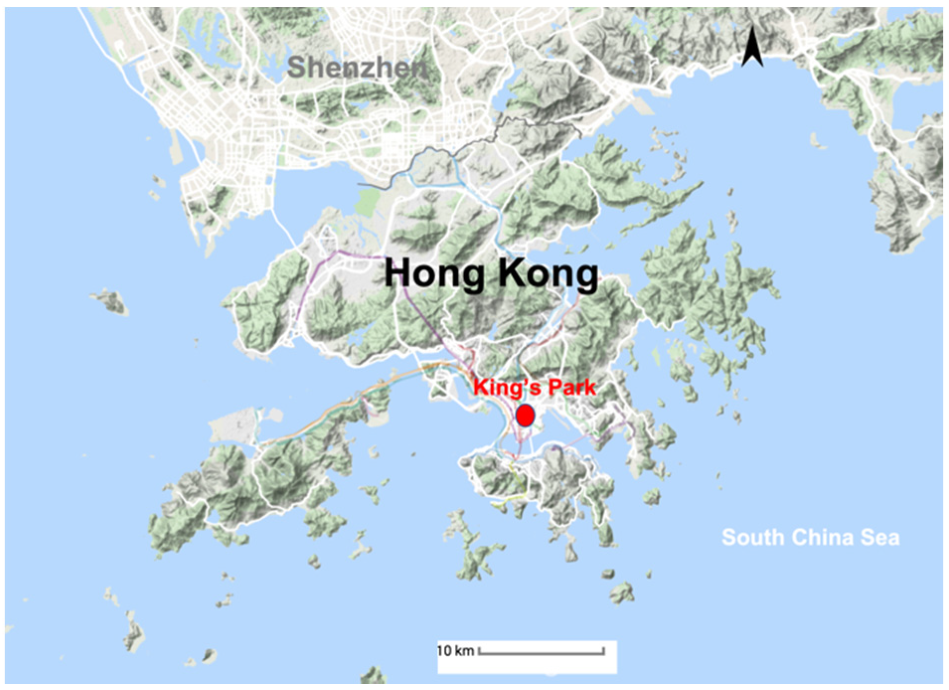
2.3. Information on the Sampling Days

Clear and cloudy days were defined according to the averaged cloud fraction between 07:00 and 17:00 HKT. Firstly, we removed the days when rainfall was recorded according to the meteorological data from HKO. 172 no-rainfall days were selected totally, accounting for 47% of all days in 2019. Of which, the average cloud fraction less than 20% were defined as clear days, whereas the remaining days were defined as cloudy days. Table 1 shows the information of the samples used in our research.

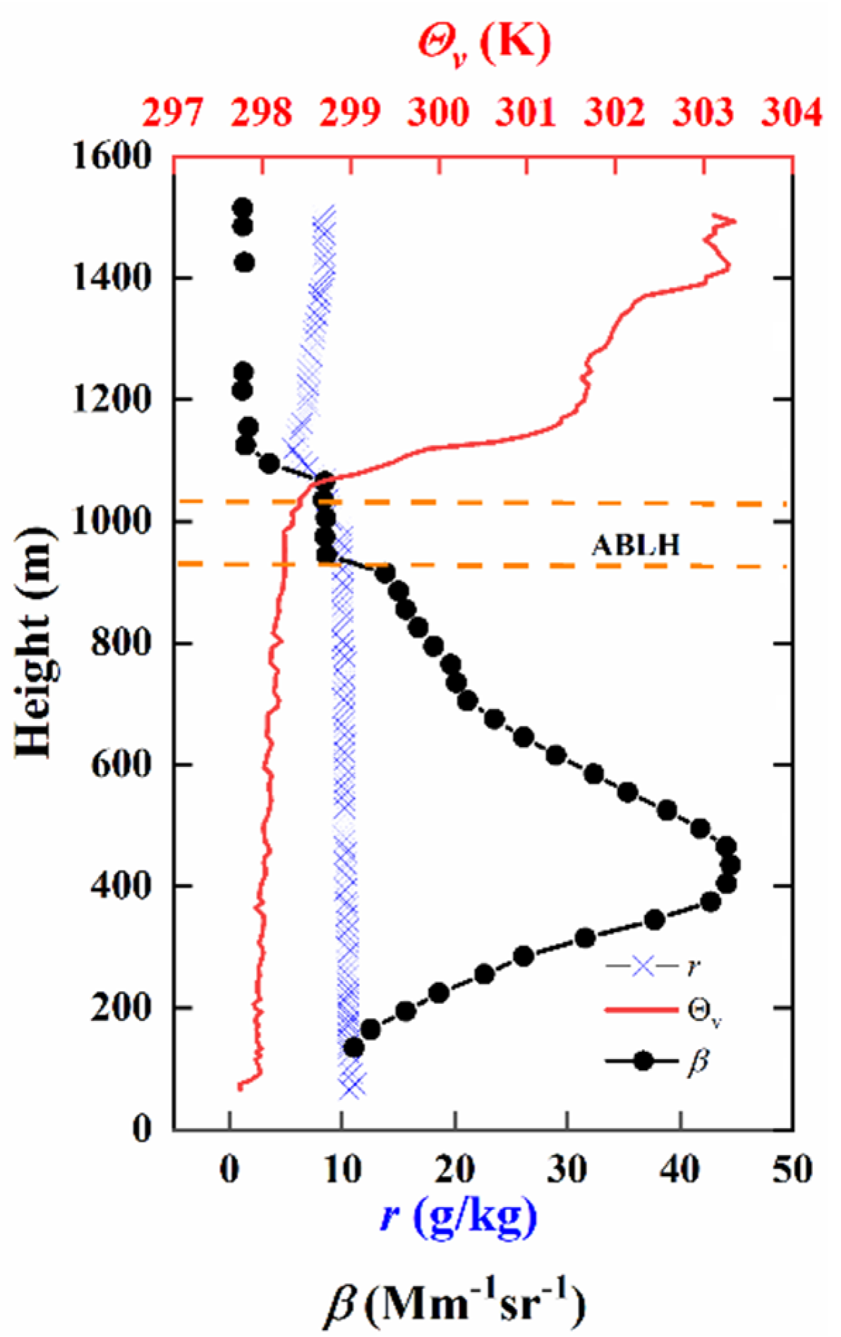
2.4. Validation of LiDAR and Definitions for Turbulent Mixing

Wind profile of our LiDAR has been well validated in 3DREAMS. Moreover, ABLH is also an important parameter for the LiDAR’s validation. Currently, there are many mature algorithms such as potential temperature gradient or Richardson number methods for radiosondes, attenuated backscatter coefficient methods for ceilometers, and particle extinction and backscatter coefficient methods for Raman and elastic LiDARS, respectively to retrieve the ABLH [40,41]. Some newly developed algorithms also obtained finer results for this purpose [42,43,44]. In order to verify the accuracy of the retrieval ABL from our LiDAR, here we applied the gradient method in the profile of water vapor mixing ratio and virtual potential temperature from regular sounding data to compare with the gradient of our attenuated backscatter coefficient (i.e., maximum - β , as β   should   always   be   negative ) on a clear case: 08:00 HKT (UTC 00) 16 October (surface wind speed: 4 m/s; wind direction: Northeast; temperature: 24.2 °C; Cloud fraction: 0). An attenuated backscatter coefficient profile should be moving averaged using a time window of 3 min and vertical window of 3 layers [22,32]. The ABLHs retrieved based on LiDAR’s attenuated backscatter coefficients and upper air sounding profiles of water vapor mixing ratio and virtual potential temperature show good consistency (Figure 2), confirming the accuracy of our LiDAR’s capacity in clear-sky ABLH retrieval.
The turbulent mixing was typically defined as the vertical velocity variance σ w 2 ( z ) within 1 minute higher than a threshold of 0.1 m2s−2 at a certain layer [31]. Therefore, here the definitions of variance and skewness are given:
σ w 2 ( z ) = w ( z ) 2 ¯ ,
s w ( z ) = ( w ( z ) σ w ( z ) ) 3 ¯ ,
where z is the height (m), w is the vertical wind velocity (m/s). w is the deviation between instant vertical velocity and the mean. As s w ( z ) is a noisy profile, a 10-min moving average was applied for the visualization in Figure 7. Correspondingly, the 1-min skewness s w ( z ) of vertical velocity was also calculated to represent the sources of turbulent mixing [4,32]. If s w ( z ) > 0, the mixing is induced by surface heating and vertical wind shear processes. If s w ( z ) < 0, the mixing is induced by cloud-driven ones.
Wind shear was found to play an important role in a radiative-convective equilibrium system as well as in the regulating of the aerosol distribution [16,45]. It has significant effects on the momentum transport under different weather conditions, especially in a CTBL in which thermals are relatively lower than that in a clear one. Bulk vertical wind shear (VWS) was used to represent the intensity of vertical wind shear between two layers and was defined as:
VWS = ( Δ u 2 + Δ v 2 ) 1 / 2 Δ z ,
where u and v are the two components of horizontal wind, whereas Δ z is the layer thickness which was 30 m in this study. We also detected the cloud base height according to a threshold of log ( β ) > −4 and combined the method documented in Manninen’s study [32].

3. Results

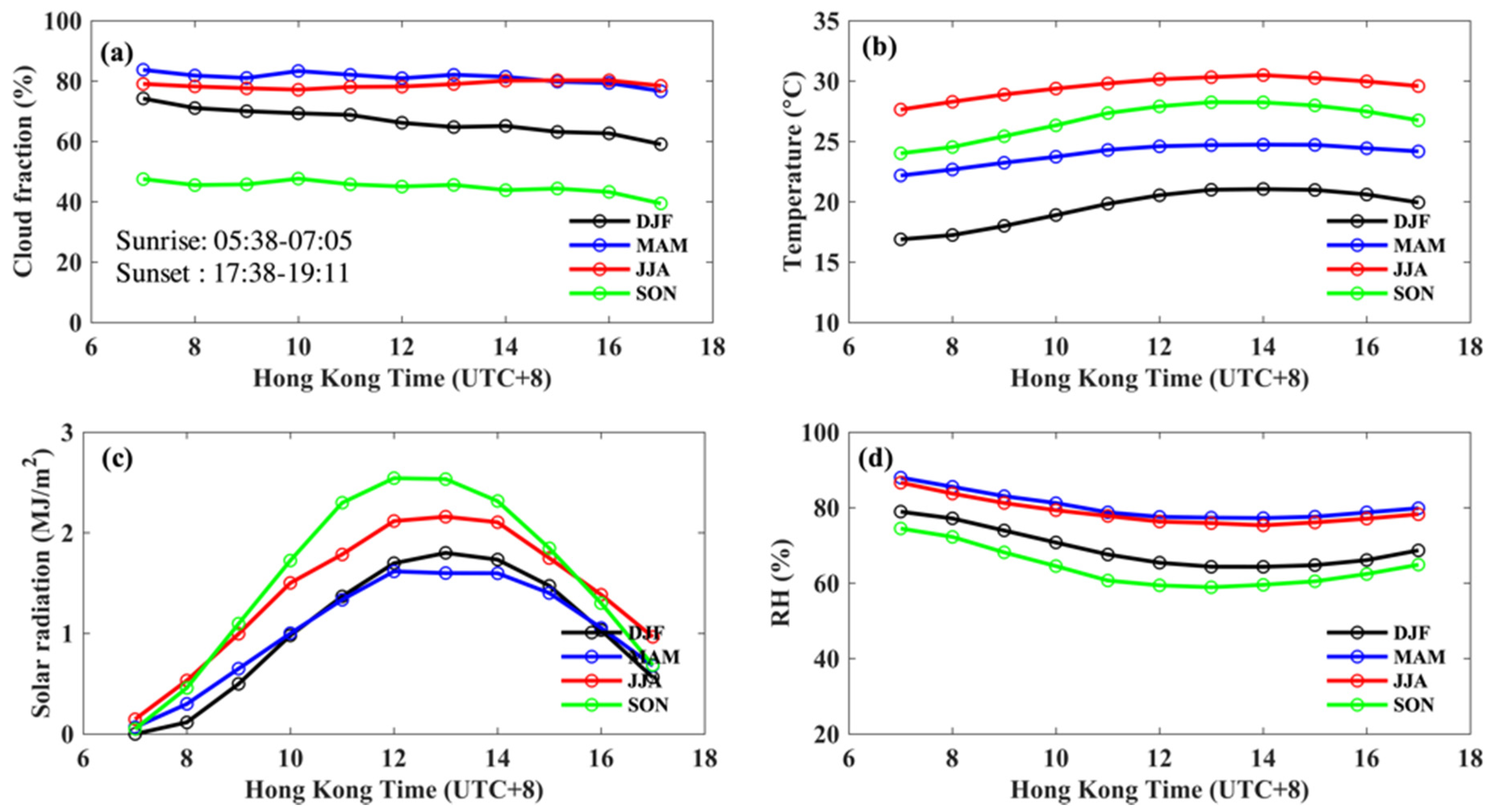
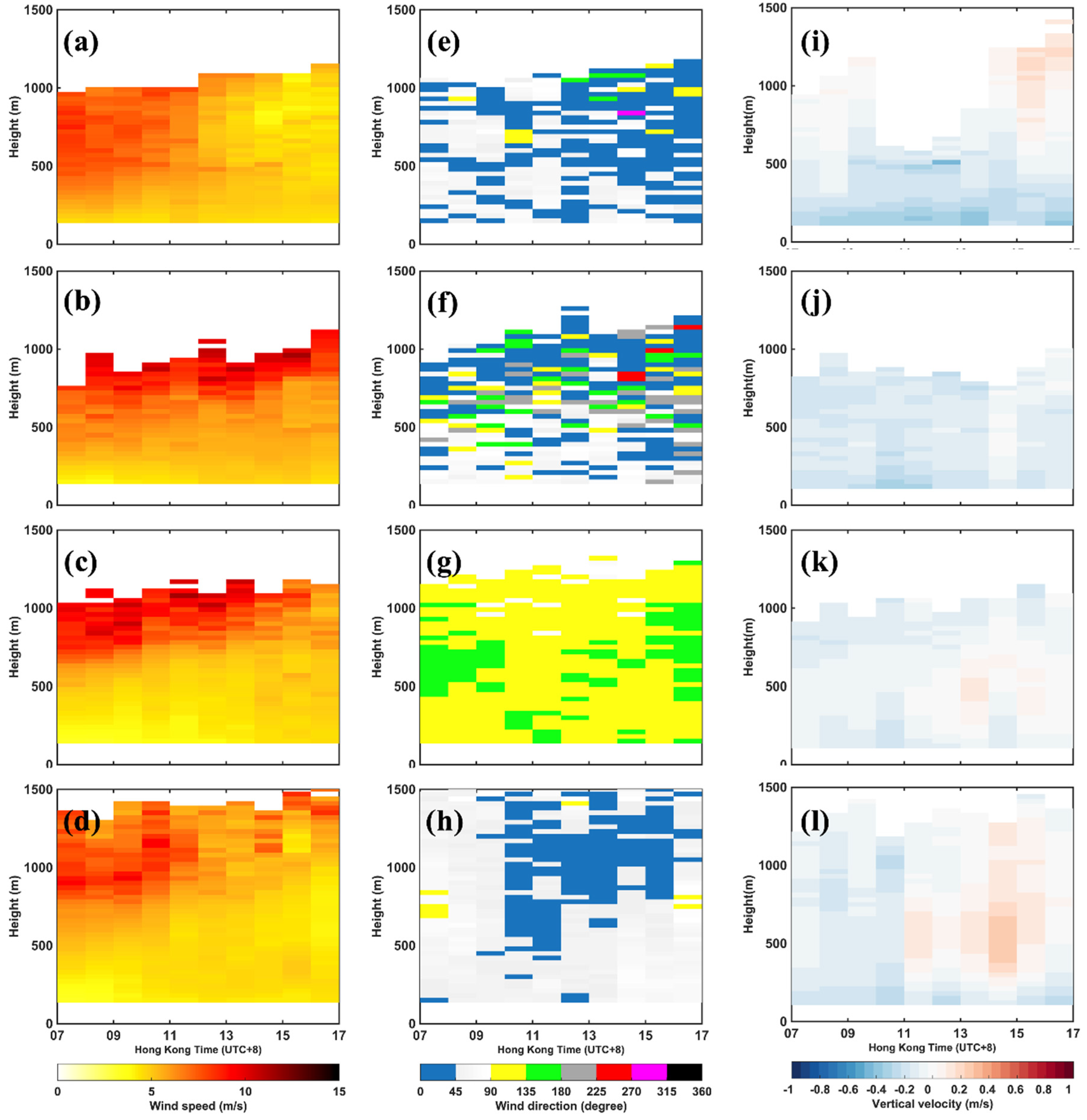
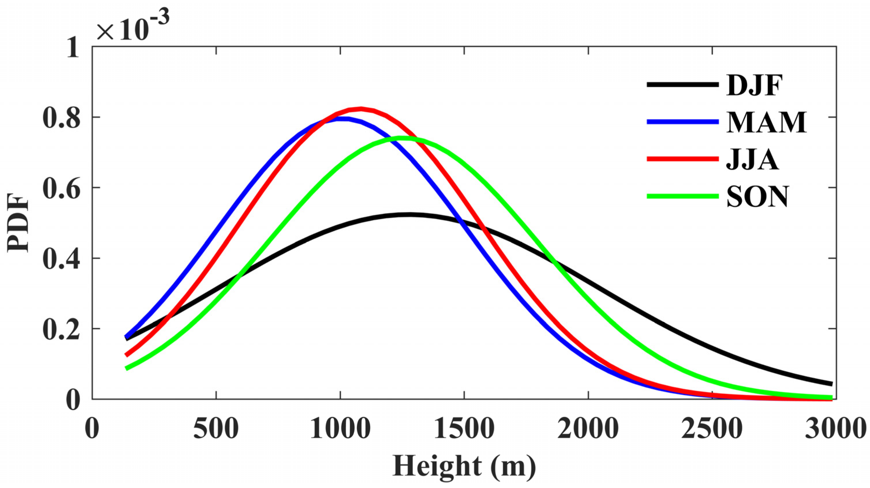
3.1. Vertical Wind Profiles and Ground-Level Meteorological Parameters on Cloudy Days in 2019

This section provides a description of meteorological conditions on cloudy days. Notably, among all the 172 no rain days in 2019, 74% of them were cloudy days. Figure 3a shows that the largest cloud fraction occurred in spring followed by summer, winter, and autumn. A similar seasonal variation was also observed in relative humidity (RH). The maximum of RH (90%) was observed at 07:00 in spring, while the minimum (60%) occurred at 13:00 in autumn. Nevertheless, the difference between maximum and minimum in each season was within 15%. In terms of solar radiation, a negative association with cloud fraction was presented. Although the temperature in summer was the highest, the higher cloud fraction in summer blocked part of solar radiation and made the surface solar radiation lower than that in autumn. Overall, cloud fraction was larger than 40% during the daytime of cloudy days in 2019, indicating that the effects associated with clouds on CTBL are ineluctable.
Figure 4 shows the diurnal variation of a cloudy-day wind profile within 1500 m in different seasons. For horizontal wind speed, the maximum occurred at 1035 m in summer with a value of 12.22 m/s at 13:00 HKT. Similarly, an obvious increase in wind speed appeared above 700 m in each season. On cloudy days, the prevailing wind direction was southeast in summer, while that was northwest in autumn and winter. Figure 4f shows that the prevailing wind direction varied significantly in spring. For vertical velocity, downdrafts were more common in spring while more updrafts were observed in autumn.
As revealed by Figure 3a, the highest cloud fraction was observed in spring while the lowest was obtained in autumn. The lower cloud fraction allowed more solar radiation reaching the ground that enhanced surface heating and thus updrafts, which were more common in the afternoon in autumn as shown in Figure 4l. Figure 5 shows the probability density function curve of cloud base height on cloudy days in different seasons. Cloud base height with the highest probability was 1395 m and 1425 m in winter and autumn, respectively, whereas that was 1095 m in spring and 1185 m in summer. The lower cloud base height in spring and summer reflected the more synoptic systems in the two seasons such as trough and typhoon, which were associated with low and thick clouds. It should also be noted that the distribution of cloud base height in winter was flatter than that in other seasons, showing the largest variations in cloud base height in winter.

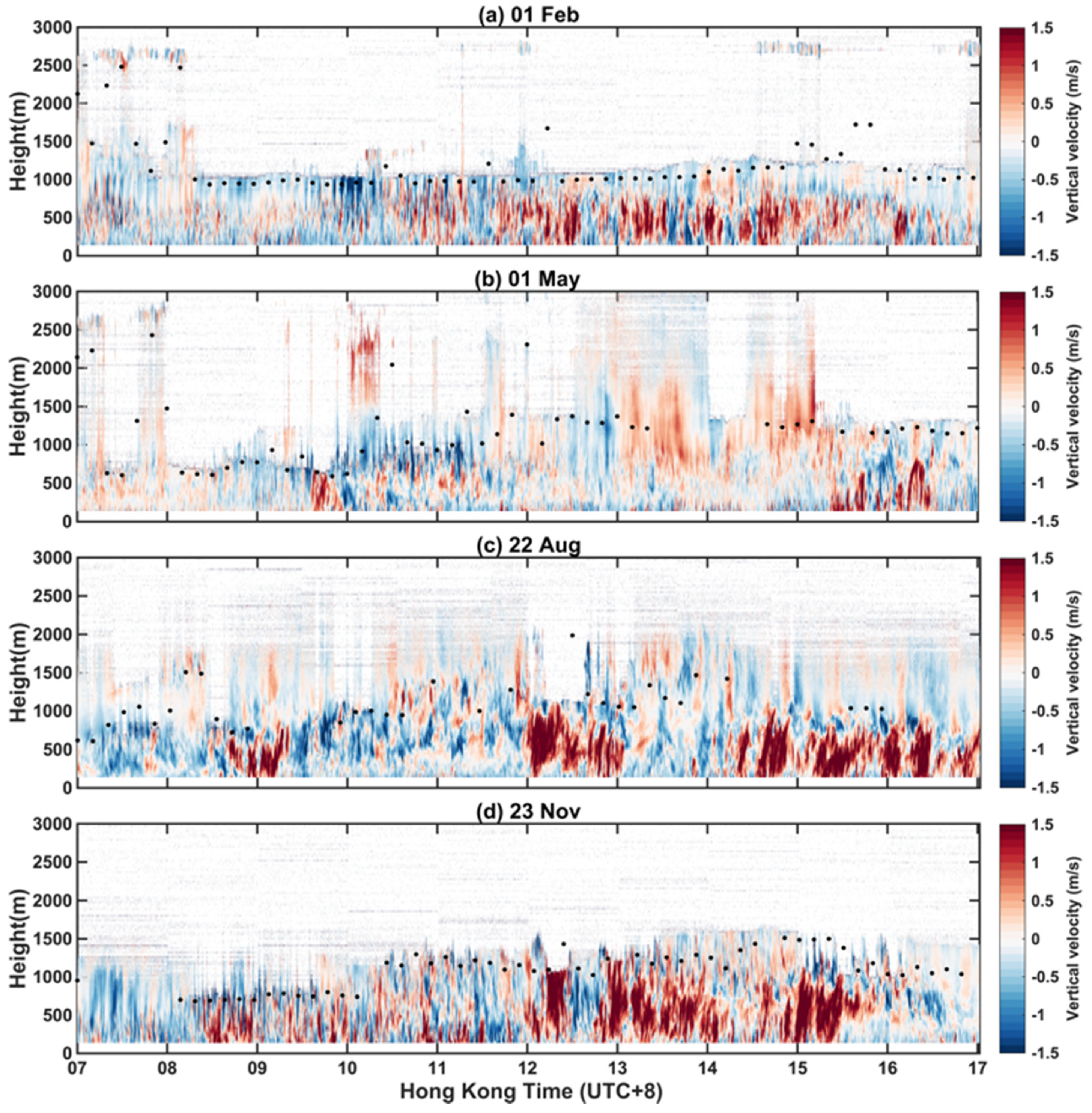
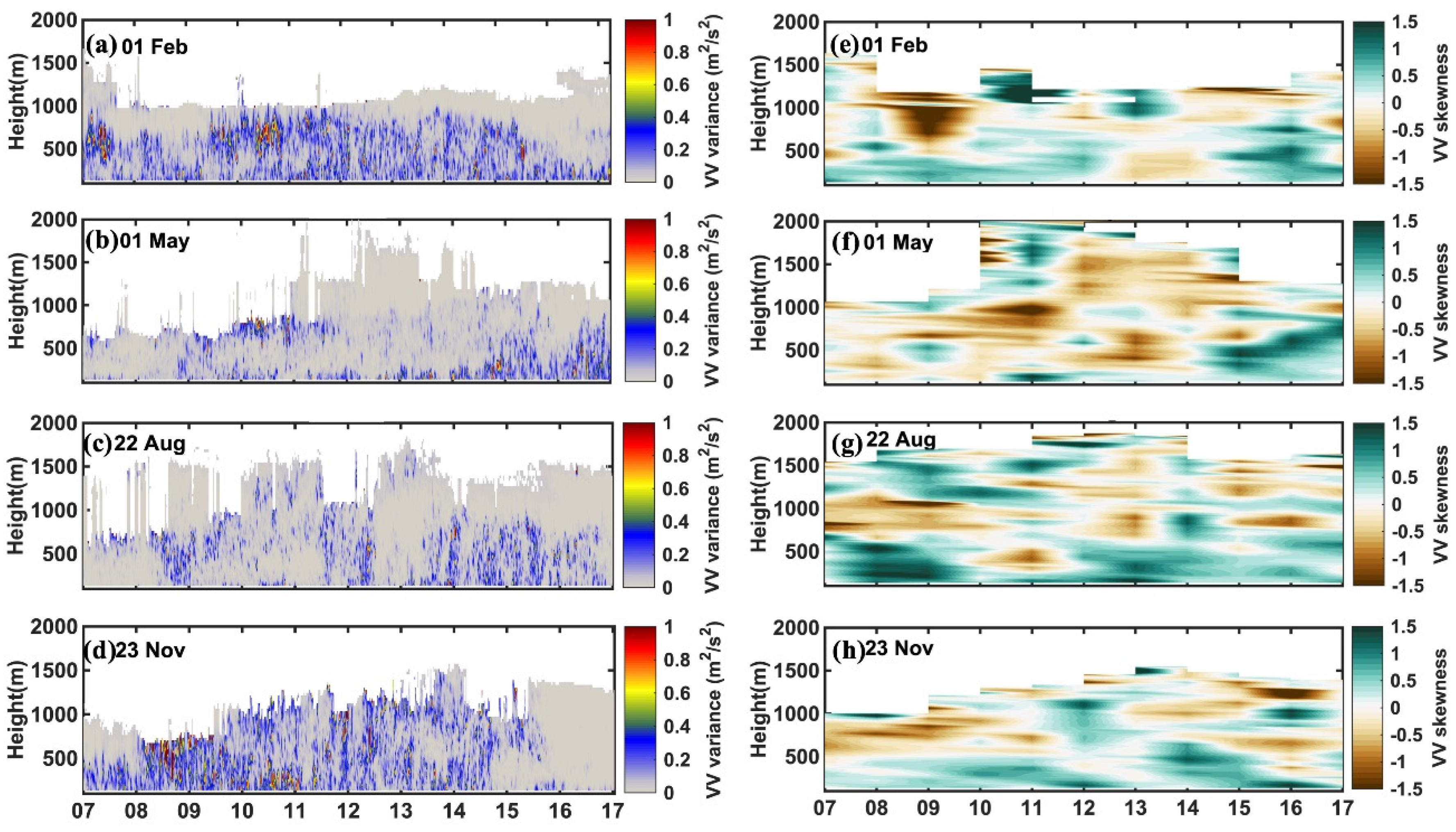
3.2. Case Study of Vertical Velocity and Turbulent Mixing Characteristics

To assess vertical velocity and turbulent mixing characteristics on cloudy days, four cases with high cloud fraction and thick clouds in different seasons were selected for a detailed analysis. The four cases included 1 Feb, 1 May, 22 Aug and 23 Nov. Figure 6 shows the vertical velocity profiles from 07:00 to 17:00 HKT in the four cases. 10-min cloud base height derived from attenuated backscatter coefficient was marked as black dots. As shown in the results, evident downdrafts were observed under the cloud base especially during 10:00 to 10:30 on 01 Feb, 10:00 to 12:00 on 01 May, 09:30 to 12:00 on 22 Aug and 16:00 to 17:00 on 23 Nov. Some evident red patches occurred in each case might be driven by relatively strong surface heating at that time. These characteristics further confirm that cloud-induced radiative cooling is one of the main sources of downdrafts during the daytime on cloudy days.
To further understand the characteristics of turbulent mixing in the CTBL, the variance and skewness of the 1-min interval vertical velocity were calculated. Figure 7 (left panels) shows significant vertical velocity variances ( σ w 2 > 0.1), implying the significant turbulent mixing generated from the near-surface layer to the bottom of clouds. Figure 7 (right panels) shows the skewness in the four cases. Three sources (i.e., cloud radiative cooling, surface heating and vertical wind shear) were considered as the main driving forces of turbulent mixing in the CTBL. It is noted that negative skewness implies the turbulent mixing due to cloud radiative cooling whereas the positive one implies that the turbulent mixing was induced by surface heating, vertical wind shear, or a combination of them [32]. As expected, turbulent mixing near the ground surface was dominantly controlled by positive skewness. Nevertheless, the negative skewness was also evidently observed especially in Figure 7f,g. In the variance of these two cases, a clear weaker variance was derived where there was negative skewness compared to the place where skewness was positive. This may imply that surface heating and vertical wind shear are relatively larger than cloud radiative cooling effect in terms of contribution to turbulent mixing.

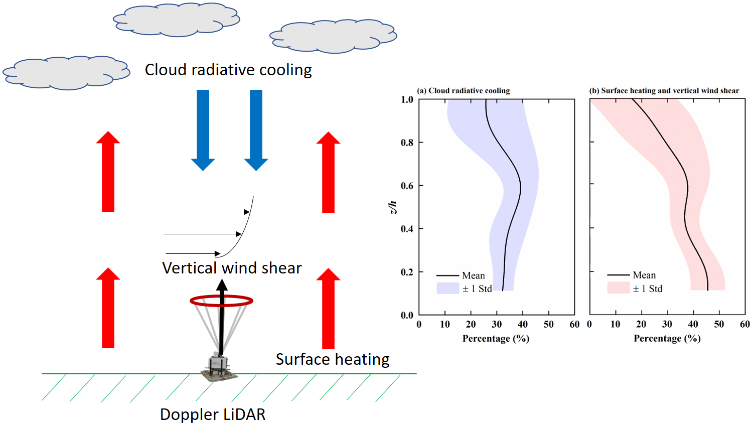
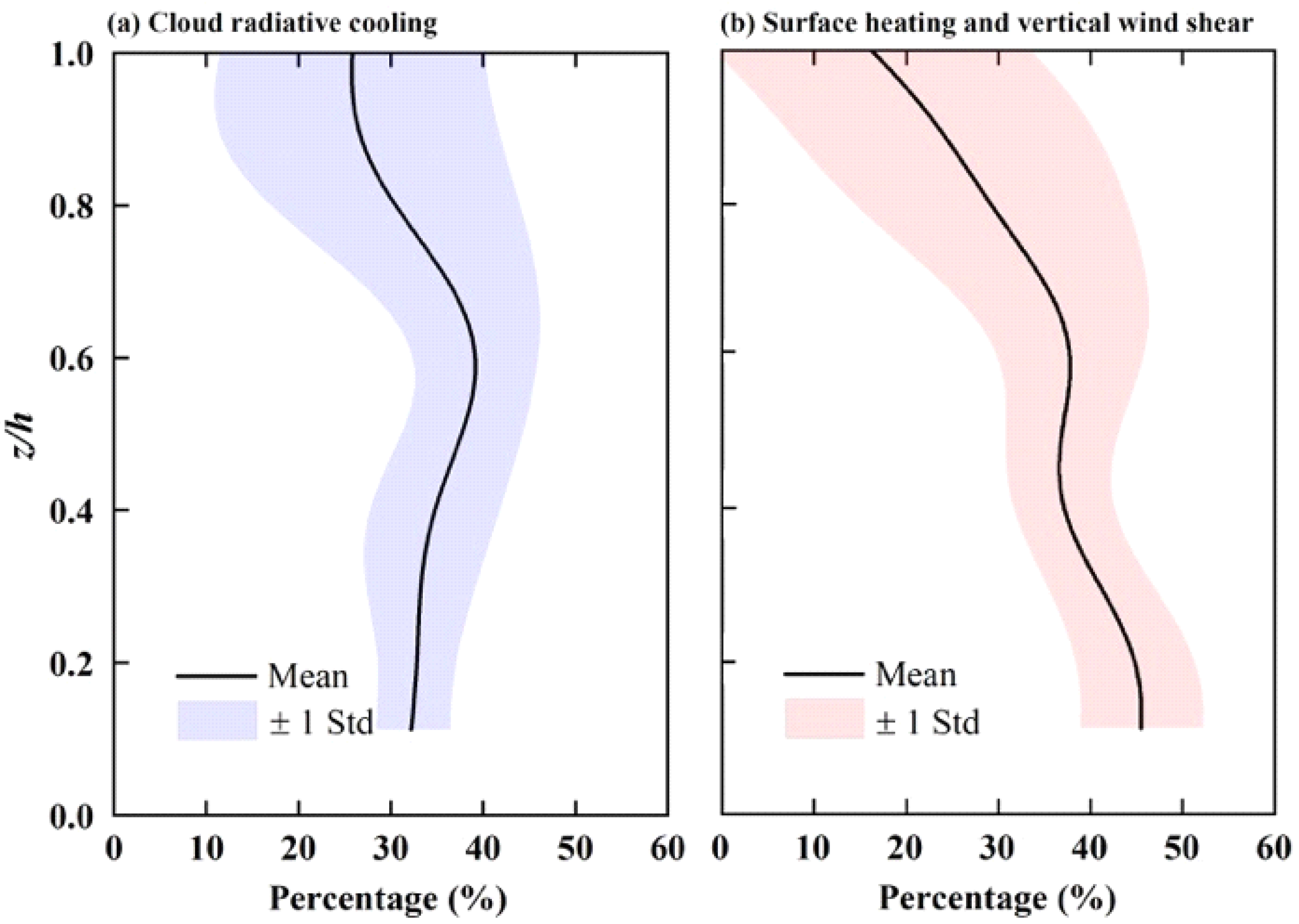
3.3. Cloud Contribution to the Turbulent Mixing

To further reveal the contribution of cloud radiative cooling to the intensity of turbulent mixing in different layers in the CTBL, we calculated the proportion of variance with a negative skewness to represent cloud contribution in Figure 8a and with a positive skewness to represent surface heating and vertical wind shear in Figure 8b, respectively. Note that the sum of the two contributions was not equal to 1 as there were many blank zones in the skewness profile where the value was 0. This part was also reflected by Manninen et al. who called this phenomenon as intermittent [32]. Figure 8a shows that cloud radiative cooling contributed ~32% to the turbulent mixing near the surface. It was comparable with the one from surface heating and vertical wind shear. The contribution of cloud-topped cooling increased with the height, but the peak emerged at ~800 m and then the contribution started to decrease again. One explanation is that most clouds in these four cases appeared at around 1000 m or even lower (see Figure 6a–c), and the cloud-topped region can be affected by the entrainment of warm and dry air from above the cloud and the turbulent instability, which has recently been studied by Mellado et al. [46]. Figure 8b explains that the overall contribution of surface heating and vertical wind shear to the turbulent mixing in each layer decreased with height, with the highest mean value of 45% near the surface. Meanwhile, the standard deviation tended to be larger especially above 800 m, indicating that the significant contribution was up to that height.
Except for cloud radiative cooling, both surface heating and vertical wind shear have significant impacts on the turbulent mixing. Hence, we further distinguished the effects of these two factors. Figure 9 shows the daytime mean intensity of vertical wind shear between different levels in each case. The highest magnitude of wind shear always occurred between two nearest layers (i.e., 30 m in our study). A significant increase was observed in each profile at ~600 m to 1000 m. The magnitude above this layer height stayed higher than that near-surface. This result reveals that, on cloudy days, the contribution of vertical wind shear on turbulent mixing was more significant aloft than near the surface.
Figure 10 depicts the correlation between turbulent mixing and surface heating due to solar radiation and vertical wind shear. In Figure 10a, surface radiation was used to represent the level of surface heat flux. Significant correlation coefficients were derived from 135 m to 435 m and from 855 m to 975 m, respectively. The appearance of the high-level significant correlation may be still induced by the entrainment discussed above, which was associated with the temperature inversion, resulting in the adverse direction of the reducing effect from surface heating. Figure 10a also shows that, in a typical daytime CTBL, surface heating significantly contributed to the turbulent mixing up to 435 m from ground level. On the other hand, in Figure 10b, vertical wind shear was calculated between every two consecutive layers (30 m). A much higher correlation coefficient can be derived in Figure 10b compared to Figure 10a. Moreover, significant results can reach up to 1095 m in a typical daytime CTBL, indicating that vertical wind shear (mechanical process) played a more important role than surface heating in a CTBL.

4. Discussion

Since Hong Kong is a typical coastal high-density city in the subtropics, the variations of the ABL there are complex. Due to its coastal location and complex terrain conditions, the formation and movement of clouds within the boundary layer occur often throughout a year, and its radiative cooling effect on the ground in the form of downdrafts is considerable. The findings that most clouds appeared at around 1000 m to 1500 m allowed us to figure out the regular depth of the typical CTBL in Hong Kong. Within this range, the surface heating may be important, but radiative fluxes induced by clouds produced local sources of cooling within the CTBL and can greatly influence its turbulent structure and dynamics [1]. Although we took the altitude into account, we did not categorize cloud types in detail and did not consider the situation when clouds are overlapped in the vertical direction, which may have an impact on the ABL characteristics [47].
Until now, the existing research based on observations with a high-time-resolution of the vertical wind profile gave us a general understanding of the characteristics of the turbulent mixing in a CTBL [3,11]. We can see in our results that even in the lowest layer near the surface, the cloud radiative cooling effects can still contribute ~32% of the turbulent mixing, indicating the importance of cloud-induced radiative cooling. This finding provides useful reference for turbulence and aerosol-radiation-cloud interaction research [48,49,50]. While the influence of meteorology on air quality is critical [51,52,53,54], the framework of 3DREAMS provides useful wind and aerosol backscatter data to understand air pollution, especially in the transboundary air pollution [55,56]. For example, during a transboundary air pollution (TAP) episode [56,57,58,59,60], the 3DREAMS can help us to understand the atmospheric stability, and also the contributions of cloud, buoyancy and wind shear in the local-scale vertical mixing procedure. In addition, as revealed by our results that the vertical wind shear can affect up to over 1000 m while the surface heating can only reach around 400 m in the CTBL, we should also consider the influence of wind structure on the regulating of aerosol, especially during heavy pollutant episodes. Pioneering work has been conducted by Yang et al. in 2019 [39].
The lack of direct long-time and high vertical resolution observations has brought great difficulties to atmospheric turbulence research, mesoscale weather forecasting, and thus air pollution studies. More intuitive observations, such as continuous observation of vertical wind profiles, are relatively rare. Once there is a direct observation of vertical wind profile, we can obtain the various boundary layer characteristics under different types of weather conditions, thus the research of boundary layer will have a significant improvement, which has been confirmed by Hogan et al. (2009) that long-term Doppler LiDAR observations would be useful for diagnosing the source of turbulence [11].
In general, our intention was to systematically observe and diagnose the boundary layer characteristics in Hong Kong and clarify the transfer of atmospheric energy in the boundary layer. The recently developed 3DREAMS can monitor the aerosol distribution and 3-dimension wind profile simultaneously. The monitoring of wind profiles can not only clarify the characteristics of atmospheric energy transfer but also monitor aerosols to help attribute local and transboundary air pollutions. Furthermore, our observations can also provide reliable validation data for mesoscale weather models and turbulence models. Our future monitoring will still be conducted under the framework of 3DREAMS to explore the influence of terrain on the boundary layer structure.

5. Conclusions

We employed high temporal and spatial (vertical) observations from a Doppler LiDAR to explore the turbulent mixing characteristics in the daytime cloud-topped boundary layer over Hong Kong in 2019 using 3DREAMS. Ground-level meteorological parameters and typical diurnal variation of vertical wind profile associated with clouds over Hong Kong in 2019 were derived to illustrate the cloud characteristics. Four typical cases from each season in 2019 were selected to illustrate the turbulent mixing characteristics based on the variance and skewness profiles of vertical velocity. Finally, the contribution of cloud radiative cooling, surface heating, and vertical wind shear on turbulent mixing were analyzed.
On cloudy days in 2019, the highest cloud fraction was observed in spring while the lowest was obtained in autumn. Meanwhile, downdrafts were more common in spring while more updrafts were observed in autumn, revealing that cloud radiative cooling is the main source of downdraft. On cloudy days, low-level clouds occurred generally within the range of 1000 to 1500 m. Compared to winter and autumn ones, cloud base heights were lower in spring and summer. Case studies of vertical velocity confirmed that in a typical daytime CTBL in Hong Kong, boundary layer clouds always act as the sink of heat near the bottom of the cloud layer. Although cloud radiative cooling effect on turbulent mixing was relatively weaker compared to surface heating and vertical wind shear, it still contributed ~32% even near the surface. Surface heating and vertical wind shear contributed ~45% together near the surface, but the effect of wind shear can be up to ~1100 m while that of surface heating can only reach ~450 m, revealing that vertical wind shear (mechanical process) plays a more important role than surface heating (thermal) in CTBL.
In general, our findings improved our knowledge of the turbulent mixing layer and provided useful references for weather forecast and air quality studies.

Author Contributions

Conceptualization, S.H.-l.Y.; Formal analysis, T.H., S.H.-l.Y., Y.Y., O.S.-m.L. and D.H.-y.L.; Funding acquisition, S.H.-l.Y.; Methodology, T.H.; Resources, S.H.-l.Y.; Software, J.C.-h.C.; Supervision, S.H.-l.Y.; Visualization, T.H. and Y.Y.; Writing–original draft, T.H.; Writing–review editing, S.H.-l.Y., Y.Y., O.S.-m.L., D.H.-y.L., J.C.-h.C., and J.G. All authors have read and agreed to the published version of the manuscript.

Funding

This work was jointly funded by The Vice-Chancellor’s Discretionary Fund of The Chinese University of Hong Kong (grant no. 4930744) the Early Career Scheme of Research Grants Council of Hong Kong (grant no. ECS-24301415), and the project from Environmental Sustainability and Resilience (ENSURE) partnership between CUHK and UoE (http://www.exeter.ac.uk/cuhkpartnership/).

Acknowledgments

We would like to thank the Hong Kong Observatory for providing meteorological data.

Conflicts of Interest

The authors declare no conflict of interest.

References

  1. Stull, R.B. An Introduction to Boundary Layer Meteorology; Atmospheric and Oceanographic Sciences Library; Springer: Dordrecht, The Netherlands, 1988; ISBN 978-90-277-2768-8. [Google Scholar]
  2. Seibert, P.; Beyrich, F.; Gryning, S.-E.; Joffre, S.; Rasmussen, A.; Tercier, P. Review and intercomparison of operational methods for the determination of the mixing height. Atmos. Environ. 2000, 34, 1001–1027. [Google Scholar] [CrossRef]
  3. Berg, L.K.; Newsom, R.K.; Turner, D.D. Year-Long Vertical Velocity Statistics Derived from Doppler Lidar Data for the Continental Convective Boundary Layer. J. Appl. Meteor. Climatol. 2017, 56, 2441–2454. [Google Scholar] [CrossRef]
  4. Ansmann, A.; Fruntke, J.; Engelmann, R. Updraft and downdraft characterization with Doppler lidar: Cloud-free versus cumuli-topped mixed layer. Atmos. Chem. Phys. 2010, 10, 7845–7858. [Google Scholar] [CrossRef] [Green Version]
  5. Greenhut, G.K.; Singh Khalsa, S.J. Convective Elements in the Marine Atmospheric Boundary Layer. Part I: Conditional Sampling Statistics. J. Climate Appl. Meteor. 1987, 26, 813–822. [Google Scholar] [CrossRef] [Green Version]
  6. Williams, A.G.; Hacker, J.M. The composite shape and structure of coherent eddies in the convective boundary layer. Bound.-Layer Meteorol. 1992, 61, 213–245. [Google Scholar] [CrossRef]
  7. Bretherton, C.S.; McCaa, J.R.; Grenier, H. A New Parameterization for Shallow Cumulus Convection and Its Application to Marine Subtropical Cloud-Topped Boundary Layers. Part I: Description and 1D Results. Mon. Wea. Rev. 2004, 132, 864–882. [Google Scholar] [CrossRef] [Green Version]
  8. Larson, V.E.; Schanen, D.P.; Wang, M.; Ovchinnikov, M.; Ghan, S. PDF Parameterization of Boundary Layer Clouds in Models with Horizontal Grid Spacings from 2 to 16 km. Mon. Wea. Rev. 2011, 140, 285–306. [Google Scholar] [CrossRef]
  9. Sicart, J.E. Atmospheric controls of the heat balance of Zongo Glacier (16°S, Bolivia). J. Geophys. Res. 2005, 110, D12106. [Google Scholar] [CrossRef] [Green Version]
  10. De Szoeke, S.P.; Yuter, S.; Mechem, D.; Fairall, C.W.; Burleyson, C.D.; Zuidema, P. Observations of Stratocumulus Clouds and Their Effect on the Eastern Pacific Surface Heat Budget along 20°S. J. Clim. 2012, 25, 8542–8567. [Google Scholar] [CrossRef] [Green Version]
  11. Hogan, R.J.; Grant, A.L.M.; Illingworth, A.J.; Pearson, G.N.; O’Connor, E.J. Vertical velocity variance and skewness in clear and cloud-topped boundary layers as revealed by Doppler lidar. Q. J. R. Meteorol. Soc. 2009, 135, 635–643. [Google Scholar] [CrossRef]
  12. Boers, R.; Spinhirne, J.D.; Hart, W.D. Lidar Observations of the Fine-Scale Variability of Marine Stratocumulus Clouds. J. Appl. Meteor. 1988, 27, 797–810. [Google Scholar] [CrossRef] [Green Version]
  13. Kollias, P.; Albrecht, B. The Turbulence Structure in a Continental Stratocumulus Cloud from Millimeter-Wavelength Radar Observations. J. Atmos. Sci. 2000, 57, 2417–2434. [Google Scholar] [CrossRef]
  14. Pelly, J.L.; Belcher, S.E. A mixed-layer model of the well-mixed stratocumulus-topped boundary layer. Bound. Layer Meteorol. 2001, 100, 171–187. [Google Scholar] [CrossRef]
  15. Chen, Q.; Fan, J.; Hagos, S.; Gustafson, W.I.; Berg, L.K. Roles of wind shear at different vertical levels: Cloud system organization and properties. J. Geophys. Res. Atmos. 2015, 120, 6551–6574. [Google Scholar] [CrossRef]
  16. Fan, J.; Yuan, T.; Comstock, J.M.; Ghan, S.; Khain, A.; Leung, L.R.; Li, Z.; Martins, V.J.; Ovchinnikov, M. Dominant role by vertical wind shear in regulating aerosol effects on deep convective clouds. J. Geophys. Res. Atmos. 2009, 114. [Google Scholar] [CrossRef]
  17. Guo, J.; Li, Y.; Cohen, J.B.; Li, J.; Chen, D.; Xu, H.; Liu, L.; Yin, J.; Hu, K.; Zhai, P. Shift in the Temporal Trend of Boundary Layer Height in China Using Long-Term (1979–2016) Radiosonde Data. Geophys. Res. Lett. 2019, 46, 6080–6089. [Google Scholar] [CrossRef] [Green Version]
  18. Lenschow, D.H.; Sun, J. The spectral composition of fluxes and variances over land and sea out to the mesoscale. Bound. Layer Meteorol. 2007, 125, 63–84. [Google Scholar] [CrossRef] [Green Version]
  19. Martin, S.; Beyrich, F.; Bange, J. Observing Entrainment Processes Using a Small Unmanned Aerial Vehicle: A Feasibility Study. Bound. Layer Meteorol. 2014, 150, 449–467. [Google Scholar] [CrossRef]
  20. Su, T.; Li, J.; Li, C.; Xiang, P.; Lau, A.K.-H.; Guo, J.; Yang, D.; Miao, Y. An intercomparison of long-term planetary boundary layer heights retrieved from CALIPSO, ground-based lidar, and radiosonde measurements over Hong Kong. J. Geophys. Res. Atmos. 2017, 122, 3929–3943. [Google Scholar] [CrossRef]
  21. Liu, B.; Ma, Y.; Guo, J.; Gong, W.; Zhang, Y.; Mao, F.; Li, J.; Guo, X.; Shi, Y. Boundary Layer Heights as Derived From Ground-Based Radar Wind Profiler in Beijing. IEEE Trans. Geosci. Remote Sens. 2019, 57, 8095–8104. [Google Scholar] [CrossRef]
  22. Tang, G.; Zhang, J.; Zhu, X.; Song, T.; Münkel, C.; Hu, B.; Schäfer, K.; Liu, Z.; Zhang, J.; Wang, L.; et al. Mixing layer height and its implications for air pollution over Beijing, China. Atmos. Chem. Phys. 2016, 16, 2459–2475. [Google Scholar] [CrossRef] [Green Version]
  23. Lolli, S.; Delaval, A.; Loth, C.; Garnier, A.; Flamant, P.H. 0.355-micrometer direct detection wind lidar under testing during a field campaign in consideration of ESA’s ADM-Aeolus mission. Atmos. Meas. Tech. 2013, 6, 3349–3358. [Google Scholar] [CrossRef] [Green Version]
  24. Lolli, S.; Khor, W.Y.; Matjafri, M.Z.; Lim, H.S. Monsoon Season Quantitative Assessment of Biomass Burning Clear-Sky Aerosol Radiative Effect at Surface by Ground-Based Lidar Observations in Pulau Pinang, Malaysia in 2014. Remote Sens. 2019, 11, 2660. [Google Scholar] [CrossRef] [Green Version]
  25. Illingworth, A.J.; Hogan, R.J.; O’Connor, E.J.; Bouniol, D.; Brooks, M.E.; Delanoé, J.; Donovan, D.P.; Eastment, J.D.; Gaussiat, N.; Goddard, J.W.F.; et al. Cloudnet: Continuous Evaluation of Cloud Profiles in Seven Operational Models Using Ground-Based Observations. Bull. Am. Meteorol. Soc. 2007, 88, 883–898. [Google Scholar] [CrossRef] [Green Version]
  26. Boesenberg, J.; Matthias, V.; Amodeo, A.; Amoiridis, V.; Ansmann, A.; Baldasano, J.M.; Balin, I.; Balis, D.; Bockmann, C.; Boselli, A.; et al. EARLINET: A European Aerosol Research Lidar Network to Establish an Aerosol Climatology; Report/Max-Planck-Institut für Meteorologie, No. 348: Hamburg, Germany, 2003. [Google Scholar] [CrossRef]
  27. Weisshaupt, N.; Arizaga, J.; Maruri, M. The role of radar wind profilers in ornithology. Ibis 2018, 160, 516–527. [Google Scholar] [CrossRef] [Green Version]
  28. Crenn, V.; Sciare, J.; Croteau, P.L.; Verlhac, S.; Fröhlich, R.; Belis, C.A.; Aas, W.; Äijälä, M.; Alastuey, A.; Artiñano, B.; et al. ACTRIS ACSM intercomparison—Part 1: Reproducibility of concentration and fragment results from 13 individual Quadrupole Aerosol Chemical Speciation Monitors (Q-ACSM) and consistency with co-located instruments. Atmos. Meas. Tech. 2015, 8, 5063–5087. [Google Scholar] [CrossRef] [Green Version]
  29. Behrendt, A.; Nakamura, T.; Onishi, M.; Baumgart, R.; Tsuda, T. Combined Raman lidar for the measurement of atmospheric temperature, water vapor, particle extinction coefficient, and particle backscatter coefficient. Appl. Opt. AO 2002, 41, 7657–7666. [Google Scholar] [CrossRef]
  30. Snels, M.; Cairo, F.; Colao, F.; Donfrancesco, G.D. Calibration method for depolarization lidar measurements. Int. J. Remote Sens. 2009, 30, 5725–5736. [Google Scholar] [CrossRef]
  31. Pearson, G.; Davies, F.; Collier, C. Remote sensing of the tropical rain forest boundary layer using pulsed Doppler lidar. Atmos. Chem. Phys. 2010, 10, 5891–5901. [Google Scholar] [CrossRef] [Green Version]
  32. Manninen, A.J.; Marke, T.; Tuononen, M.; O’Connor, E.J. Atmospheric boundary layer classification with doppler lidar. J. Geophys. Res. Atmos. 2018, 123, 8172–8189. [Google Scholar] [CrossRef]
  33. Yim, S.H.L. Development of a 3D Real-Time Atmospheric Monitoring System (3DREAMS) Using Doppler LiDARs and Applications for Long-Term Analysis and Hot-and-Polluted Episodes. Remote Sens. 2020, 12, 1036. [Google Scholar] [CrossRef] [Green Version]
  34. Milroy, C.; Martucci, G.; Lolli, S.; Loaec, S.; Sauvage, L.; Xueref-Remy, I.; Lavrič, J.V.; Ciais, P.; Feist, D.G.; Biavati, G.; et al. An assessment of pseudo-operational ground-based light detection and ranging sensors to determine the boundary-layer structure in the coastal atmosphere. Adv. Meteorol. 2012, 2012, 929080. [Google Scholar] [CrossRef] [Green Version]
  35. Barlow, J.F.; Dunbar, T.M.; Nemitz, E.G.; Wood, C.R.; Gallagher, M.W.; Davies, F.; O’Connor, E.; Harrison, R.M. Boundary layer dynamics over London, UK, as observed using Doppler lidar during REPARTEE-II. Atmos. Chem. Phys. 2011, 11, 2111–2125. [Google Scholar] [CrossRef] [Green Version]
  36. De Arruda Moreira, G.; Da Silva Lopes, F.J.; Guerrero-Rascado, J.L.; João Da Silva, J.; Gomes, A.A.; Landulfo, E.; Alados-Arboledas, L. Analyzing the atmospheric boundary layer using high-order moments obtained from multiwavelength lidar data: Impact of wavelength choice. Atmos. Meas. Tech. 2019, 12, 4261–4276. [Google Scholar] [CrossRef] [Green Version]
  37. De Arruda Moreira, G.; Guerrero-Rascado, J.L.; Bravo-Aranda, J.A.; Benavent-Oltra, J.A.; Ortiz-Amezcua, P.; Róman, R.; Bedoya-Velásquez, A.E.; Landulfo, E.; Alados-Arboledas, L. Study of the planetary boundary layer by microwave radiometer, elastic lidar and Doppler lidar estimations in Southern Iberian Peninsula. Atmos. Res. 2018, 213, 185–195. [Google Scholar] [CrossRef] [Green Version]
  38. Yang, D.; Li, C.; Lau, A.K.-H.; Li, Y. Long-term measurement of daytime atmospheric mixing layer height over Hong Kong. J. Geophys. Res. Atmos. 2013, 118, 2422–2433. [Google Scholar] [CrossRef]
  39. Yang, Y.; Yim, S.H.L.; Haywood, J.; Osborne, M.; Chan, J.C.S.; Zeng, Z.; Cheng, J.C.H. Characteristics of Heavy particulate matter pollution events over hong kong and their relationships with vertical wind profiles using high-time-resolution doppler lidar measurements. J. Geophys. Res. Atmos. 2019, 124, 9609–9623. [Google Scholar] [CrossRef] [Green Version]
  40. Melfi, S.H.; Whiteman, D.; Ferrare, R. Observation of Atmospheric Fronts Using Raman Lidar Moisture Measurements. J. Appl. Meteorol. 1989, 28, 789–806. [Google Scholar] [CrossRef] [Green Version]
  41. Ansmann, A.; Wandinger, U.; Riebesell, M.; Weitkamp, C.; Michaelis, W. Independent measurement of extinction and backscatter profiles in cirrus clouds by using a combined Raman elastic-backscatter lidar. Appl. Opt. AO 1992, 31, 7113–7131. [Google Scholar] [CrossRef]
  42. Morille, Y.; Haeffelin, M.; Drobinski, P.; Pelon, J. STRAT: An Automated Algorithm to Retrieve the Vertical Structure of the Atmosphere from Single-Channel Lidar Data. J. Atmos. Ocean. Technol. 2007, 24, 761–775. [Google Scholar] [CrossRef] [Green Version]
  43. De Bruine, M.; Apituley, A.; Donovan, D.P.; Klein Baltink, H.; de Haij, M.J. Pathfinder: Applying graph theory to consistent tracking of daytime mixed layer height with backscatter lidar. Atmos. Meas. Tech. 2017, 10, 1893–1909. [Google Scholar] [CrossRef] [Green Version]
  44. Geiß, A.; Wiegner, M.; Bonn, B.; Schäfer, K.; Forkel, R.; von Schneidemesser, E.; Münkel, C.; Chan, K.L.; Nothard, R. Mixing layer height as an indicator for urban air quality? Atmos. Meas. Tech. 2017, 10, 2969–2988. [Google Scholar] [CrossRef] [Green Version]
  45. Zhang, Y.; Guo, J.; Yang, Y.; Wang, Y.; Yim, S. Vertical Wind Shear Modulates Particulate Matter Pollutions: A Perspective from Radar Wind Profiler Observations in Beijing, China. Remote Sens. 2020, 12, 546. [Google Scholar] [CrossRef] [Green Version]
  46. Mellado, J.P. Cloud-Top Entrainment in Stratocumulus Clouds. Annu. Rev. Fluid Mech. 2017, 49, 145–169. [Google Scholar] [CrossRef]
  47. Dang, R.; Yang, Y.; Li, H.; Hu, X.-M.; Wang, Z.; Huang, Z.; Zhou, T.; Zhang, T. Atmosphere Boundary Layer Height (ABLH) Determination under Multiple-Layer Conditions Using Micro-Pulse Lidar. Remote Sens. 2019, 11, 263. [Google Scholar] [CrossRef] [Green Version]
  48. Liu, Z.; Ming, Y.; Zhao, C.; Lau, N.C.; Guo, J.; Bollasina, M.; Yim, S.H.L. Contribution of local and remote anthropogenic aerosols to a record-breaking torrential rainfall event in Guangdong Province, China. Atmos. Chem. Phys. 2020, 20, 223–241. [Google Scholar] [CrossRef] [Green Version]
  49. Liu, Z.; Ming, Y.; Wang, L.; Bollasina, M.; Luo, M.; Lau, N.-C.; Yim, S.H.-L. A Model Investigation of Aerosol-Induced Changes in the East Asian Winter Monsoon. Geophys. Res. Lett. 2019, 46, 10186–10195. [Google Scholar] [CrossRef] [Green Version]
  50. Liu, Z.; Yim, S.H.L.; Wang, C.; Lau, N.C. The Impact of the Aerosol Direct Radiative Forcing on Deep Convection and Air Quality in the Pearl River Delta Region. Geophys. Res. Lett. 2018, 45, 4410–4418. [Google Scholar] [CrossRef]
  51. Yim, S.H.L.; Wang, M.; Gu, Y.; Yang, Y.; Dong, G.; Li, Q. Effect of urbanization on ozone and resultant health effects in the pearl river delta region of China. J. Geophys. Res. Atmos. 2019, 124, 11568–11579. [Google Scholar] [CrossRef]
  52. Tong, C.H.M.; Yim, S.H.L.; Rothenberg, D.; Wang, C.; Lin, C.-Y.; Chen, Y.D.; Lau, N.C. Projecting the impacts of atmospheric conditions under climate change on air quality over the Pearl River Delta region. Atmos. Environ. 2018, 193, 79–87. [Google Scholar] [CrossRef]
  53. Tong, C.H.M.; Yim, S.H.L.; Rothenberg, D.; Wang, C.; Lin, C.-Y.; Chen, Y.; Lau, N.C. Assessing the impacts of seasonal and vertical atmospheric conditions on air quality over the Pearl River Delta region. Atmos. Environ. 2018, 180, 69–78. [Google Scholar] [CrossRef]
  54. Yim, S.H.L.; Fung, J.C.H.; Ng, E.Y.Y. An assessment indicator for air ventilation and pollutant dispersion potential in an urban canopy with complex natural terrain and significant wind variations. Atmos. Environ. 2014, 94, 297–306. [Google Scholar] [CrossRef]
  55. Shi, C.; Nduka, I.C.; Yang, Y.; Huang, Y.; Yao, R.; Zhang, H.; He, B.; Xie, C.; Wang, Z.; Yim, S.H.L. Characteristics and meteorological mechanisms of transboundary air pollution in a persistent heavy PM2.5 pollution episode in Central-East China. Atmos. Environ. 2020, 223, 117239. [Google Scholar] [CrossRef]
  56. Gu, Y.; Yim, S.H.L. The air quality and health impacts of domestic trans-boundary pollution in various regions of China. Environ. Int. 2016, 97, 117–124. [Google Scholar] [CrossRef] [PubMed]
  57. Hou, X.; Chan, C.K.; Dong, G.H.; Yim, S.H.L. Impacts of transboundary air pollution and local emissions on PM2.5 pollution in the Pearl River Delta region of China and the public health, and the policy implications. Environ. Res. Lett. 2018. [Google Scholar] [CrossRef]
  58. Yim, S.H.L.; Gu, Y.; Shapiro, M.A.; Stephens, B. Air quality and acid deposition impacts of local emissions and transboundary air pollution in Japan and South Korea. Atmos. Chem. Phys. 2019, 19, 13309–13323. [Google Scholar] [CrossRef] [Green Version]
  59. Luo, M.; Hou, X.; Gu, Y.; Lau, N.-C.; Yim, S.H.-L. Trans-boundary air pollution in a city under various atmospheric conditions. Sci. Total Environ. 2018, 618, 132–141. [Google Scholar] [CrossRef]
  60. Yim, S.H.L.; Hou, X.; Guo, J.; Yang, Y. Contribution of local emissions and transboundary air pollution to air quality in Hong Kong during El Niño-Southern Oscillation and heatwaves. Atmos. Res. 2019, 218, 50–58. [Google Scholar] [CrossRef]
Figure 1. Location (red dot) of the LiDAR at King’s Park (LiDAR KP). The figure was built on a map obtained from Google map, https://www.google.com/maps.
Remotesensing 12 01533 g001
Figure 2. Vertical profiles of water vapor mixing ratio r (blue cross), virtual potential temperature θ v (red line), and attenuated backscatter coefficient (black dot) at 08:00 Hong Kong Time (HKT) (UTC 00) on 16 October. The range of atmospheric boundary layer height (ABLH) has been marked with orange dash lines.
Remotesensing 12 01533 g002
Figure 3. Diurnal variation of meteorological parameters of (a) cloud fraction, (b) temperature, (c) solar radiation, and (d) relative humidity (RH) from ground-level observation data at King’s Park Meteorological Station (KPMS) on cloudy days in 2019. Sunrise and sunset marked in the figure were extracted from the Hong Kong Observatory website (https://www.hko.gov.hk/tc/gts/astron2019/almanac2019_index.htm). A t-test for the differences between seasons was conducted. The t-test results show that all the seasonal differences can pass a 95% test except the solar radiation difference between winter and spring (p < 0.2) and RH difference between spring and summer (p < 0.3).
Remotesensing 12 01533 g003
Figure 4. Diurnal variation of wind profiles of horizontal wind speed (left), horizontal wind direction (middle), and vertical velocity (right) on cloudy days in 2019. The rows from top to bottom represent winter, spring, summer and autumn, respectively.
Remotesensing 12 01533 g004
Figure 5. The probability distribution function of cloud base height within the atmospheric boundary layer during 07:00 to 17:00 HKT on cloudy days in 2019. It is noted that the curves were built based on data at a 10-min resolution.
Remotesensing 12 01533 g005
Figure 6. Vertical velocity profiles from 07:00 to 17:00 HKT on (a) 01 Feb, (b) 01 May, (c) 22 Aug, (d) 23 Nov. 10-min cloud base height has been marked as black dots in each profile. Positive vertical velocity indicates updraft.
Remotesensing 12 01533 g006
Figure 7. Vertical profile of vertical velocity variance σ w 2 (left panel) and skewness s w (right panel). Both σ w 2 and s w are 1-min time interval. For visualization, s w has been moving averaged in a 10-min window size.
Remotesensing 12 01533 g007
Figure 8. Contribution of (a) cloud radiative cooling and (b) surface heating and vertical wind shear to the turbulent mixing within the daytime cloud-topped boundary layer (CTBL) in all the cases. Y axis is the altitude (z) normalized by cloud base height (h).
Remotesensing 12 01533 g008
Figure 9. Vertical profile of the averaged daytime vertical wind shear between different heights for (a) 01 Feb, (b) 01 May, (c), 22 Aug, (d) 23 Nov. Shading denotes the intensity of wind shear at least two consecutive layers where x-axis is the top layer height and y-axis is the bottom layer height. Note that the colormap is presented at a log scale.
Remotesensing 12 01533 g009
Figure 10. The correlation between turbulent mixing and the two factors: (a) surface heating due to solar radiation and (b) vertical wind shear. Solid dots represent data with high statistical significance (p < 0.05).
Remotesensing 12 01533 g010
Table 1. Numbers of no rain days and cloudy days in each season, and the percentage of no rain days with a cloudy sky.
SeasonNumber of No Rain DaysNumber of Cloudy DaysPercentage of No Rain Days with A Cloudy Sky
DJF514078%
MAM383284%
JJA252080%
SON583561%

