Article

A Spatial-Channel Collaborative Attention Network for Enhancement of Multiresolution Classification

1
The Key Laboratory of Intelligent Perception and Image Understanding of Ministry of Education, School of Artificial Intelligence, Xidian University, Xi’an 710071, China
2
The Xi’an Key Laboratory of Big Data and Intelligent Vision, Xidian University, School of Computer Science and Technology, Xi’an 710071, China
*
Author to whom correspondence should be addressed.
Submission received: 19 November 2020 / Revised: 16 December 2020 / Accepted: 21 December 2020 / Published: 30 December 2020

Abstract

:
Recently, with the popularity of space-borne earth satellites, the resolution of high-resolution panchromatic (PAN) and multispectral (MS) remote sensing images is also increasing year by year, multiresolution remote sensing classification has become a research hotspot. In this paper, from the perspective of deep learning, we design a dual-branch interactive spatial-channel collaborative attention enhancement network (SCCA-net) for multiresolution classification. It aims to combine sample enhancement and feature enhancement to improve classification accuracy. In the part of sample enhancement, we propose an adaptive neighbourhood transfer sampling strategy (ANTSS). Different from the traditional pixel-centric sampling strategy with orthogonal sampling angle, our algorithm allows each patch to adaptively transfer the neighbourhood range by finding the homogeneous region of the pixel to be classified. And it also adaptively adjust the sampling angle according to the texture distribution of the homogeneous region to capture neighbourhood information that is more conducive for classification. Moreover, in the part of feature enhancement part, we design a local spatial attention module (LSA-module) for PAN data to highlight the spatial resolution advantages and a global channel attention module (GCA-module) for MS data to improve the multi-channel representation. It not only highlights the spatial resolution advantage of PAN data and the multi-channel advantage of MS data, but also improves the difference between features through the interaction between the two modules. Quantitative and qualitative experimental results verify the robustness and effectiveness of the method.

1. Introduction

With the rapid development of earth observing technology, space-borne passive earth observation systems can jointly acquire two different images of the same scene [1]. i.e., a panchromatic image (PAN) with high spatial resolution but less spectral information, and a multi-spectral image (MS) with low spatial resolution but more spectral information [2]. Compared with the original single resolution images, the combination of these different resolution images (for brevity, we call it “multi-resolution images” ) enable users to obtain higher spatial and spectral information simultaneously. MS data is helpful for the identification of land covers, while PAN data is beneficial for accurately describing the shape and structure of objects in images. Therefore, the intrinsic complementarity between PAN and MS data conveys a vital potential for multi-resolution image classification tasks [3].
In general, the commonly used methods in PAN and MS multi-resolution classification can be roughly divided into two categories: one is first to utilize pan-sharpening to the MS data, and then classifying it [4,5,6,7,8]; the other is first to extract their respective features from PAN and MS data, and then fuse them for classification [9,10,11,12,13].
The former method is mainly to classify a fused image with the high spectral resolution and high spatial resolution, which requires an excellent pan-sharpening algorithm [14] to add the spatial details of PAN image to the MS image. Over the years, various excellent pan-sharpening algorithms have been proposed, including classical Component Substitution (e.g., Intensity-Hue-Saturation (IHS) Transformation [15,16], Principal Component Analysis (PCA) [17,18], and Gram Schmidt(GS) Transformation [19]); and Multi-Resolution Analysis (e.g., Wavelet Transform [20,21], Support Value Transform [22]).
The above methods all have good performance, and many pan-sharpening algorithms also provide many helpful inspirations for the development of image information fusion field. However, overreliance on pan-sharpening results also brings many limitations to these methods. For example, when the fusion image appeared noisy, distortion, etc., it will produce inevitable adverse effects and reduce the final classification accuracy [23].
The latter method (feature fusion then classify) usually extracts features from PAN and MS data separately, and then fuse them for classification. Zhang et al. [12] combined the mid-level bag-of-visual words model with the optimal segmentation scale to bridge the high-level semantics information and low-level detail information. These features are then sent into Support Vector Machine (SVM) for images classification. Moser et al. [11] combines a graph cut method with the linear mixed model, and iterates the relationship between PAN and MS data to generate the context classification map. Mao et al. [13] proposed a unified Bayesian framework to discover semantic segments from PAN images first, and then assign corresponding cluster labels from MS images for a significant classification result. Although these algorithms extract some features from PAN and MS data for classification, these features are only shallow features. They are easily affected by noise, which leads to unsatisfactory classification results.
During the past few years, deep learning (DL) methods have been widely used in various fields of remote sensing [24,25,26,27,28,29]. By establishing a suitable sample database and designing the hierarchical structure of the entire network carefully, it is proved that the DL algorithms can also handle the complex remote sensing data well. Zhao et al. [25] proposed a superpixel-based multiple local network model, which first perform the superpixel algorithm to generate multiple local regions samples. Multiple local network model was used to extract features of different regions samples for classification. Finally, Zhao et al. used the corresponding PAN image to fine-tune this classification results. But the algorithm use multiple local network models to extract features, all the input to the network comes from MS data, which shows that it does not explore the complementarity between MS and PAN data. Liu et al. [24] proposed a two-branch classification network based on a stacked auto-encoder (SAE) and a deep convolutional neural network (DCNN), each branch independently extracts the features of MS data and PAN data, and then through several fully-connected (FC) layers to get the final classification result. This algorithm uses a dual-path network to extract the features of MS and PAN data independently. However, the network design is too simple, and the feature representation cannot be extracted effectively for different data characteristics. Zhu et al. [27] used the spatial attention module and the channel attention module to extract the features of the PAN and MS data, respectively, then fuses them for classification. The above algorithms are well combined with the DL methods to solve the multi-resolution classification problem and improve the accuracy of multi-resolution classification, which inspires us to mine the potential of deep learning further.
Although the application of DL methods in this field has achieved impressive performance, some easily ignored problems still deserve our attention:
(1) Multi-resolution classification tasks usually perform pixel-by-pixel classification of remote sensing images containing various irregular objects in the same large scene. All sample patches have only one fixed-angle neighbourhood information, which may not be able to learn robust and distinctive feature representations. Besides, the training samples are usually image patches centred on the pixel to be classified. It will cause pixels with very close Euclidean distance but belonging to different categories to obtain very similar patch information [8,11], thereby confusing the training of the classification network.
(2) These multi-resolution images have different resolutions and spectral channels in the same scene, and usually contain local distortions, unavoidable noises, and imaging viewpoint changes. Therefore, We not only need a more powerful module to extract more robust feature representations, but also need a dual-branch network to extract features that can highlight the characteristics of their respective data. Finally, how to effectively eliminate the differences in the features obtained by the two branches and then fuse common information is also a problem that needs to be solved.
In view of the above two problems, Our main contributions includes two corresponding aspects as follows:
(1) We propose an adaptive neighbourhood transfer sampling strategy (ANTSS) to capture sample patches. For the pixel to be classified, we adaptively migrate the patch area of the pixel according to its homogeneous structure. Moreover, the clipping angle of the patch is not fixed and is adaptively determined by the edge texture structure of its homogeneous area, so that it can better deal with objects of different shapes. And this patch tends to contain more texture information that is homogeneous with the pixel to be classified, thus effectively avoiding the above-mentioned edge categories sampling problem and providing better positive feedback for its classification.
(2) We propose an interactive attention feature fusion spatial-channel collaborative Network (SCCA-Net). In the design of the network structure, we introduce the attention mechanism module into the field of remote-sensing data to expect for more robust features. We design local spatial attention (LSA-module) and global channel attention (GCA-module) especially for PAN and MS data respectively, thus highlighting the spatial resolution advantages of PAN and the multi-channel advantages of MS. Finally, the interaction module effectively reduces the difference in the characteristics obtained by the PAN branch and the MS branch. Then we also use GCA-module to further enhance more in-depth feature representation from the fused features for classification.
The rest of this paper is organized as follows: Section 2 briefly introduces some related work. Section 3 elaborates the proposed method in detail. Section 4 first introduces the details of datasets used and the experimental setup, and then shows the experimental results and the corresponding analysis. Finally, Section 5 draws the conclusion of this paper.

2. Related Work

In this section, the sampling strategy and attention model related to our method will be introduced in detail.

2.1. Sampling Strategy

Recently, the application of deep learning in the field of remote sensing is gradually developing, but remote sensing data are often relatively large. In practical applications, it is often necessary to use raw data to make training samples. As show in the Figure 1, Liu et al. [24] and Li et al. [3], take the pixel to be classified as the centre and crop out the sample patch at an orthogonal sampling angle. The traditional pixel-centric sampling strategy is simple and easy to implement, and the sample patch containing some neighbourhood information can also extract the characteristics of some samples. However, pixel-by-pixel sampling will not only generate many similar redundant samples but also bring some confusing samples with high similarity but different categories.
Zhao et al. [25] uses the superpixel algorithm to aggregate MS data, and then takes out multiple local patches around each superpixel as a supplement to the neighbourhood information. The algorithm uses superpixels to generate sample patches, reduces many redundant samples in the training sample set, and uses auxiliary input to enhance the neighbourhood information of the category. Zhu et al. [27] employs Difference of Gaussian (DoG) scale-space [25] to capture texture structure of the multiresolution image, and then adaptively adjust the size of the patch according to the texture structure range. The algorithm captures the complete texture structure through multi-scale sample patches, which can better extract category features for classification.
However, these methods also have some problems that cannot be ignored. First of all, both traditional methods and multi-scale sampling strategies use orthogonal sliding windows to crop images. When faced with irregular edge texture structure, the orthogonal sliding window cannot effectively extract the texture information of the category. Secondly, when sampling two adjacent types of ground objects, some confusing samples with very similar neighbourhood information, but completely different categories are often obtained. Therefore, we propose an adaptive neighbourhood transfer sampling strategy (ANTSS), which can transfer the neighbourhood patch of the pixel to a region containing more homogeneous information, thereby effectively avoiding the above-mentioned edge category sampling problem. Moreover, it can adaptively adjust the clipping angle of the patch to obtain complete texture information according to the distribution of homogeneous regions.

2.2. Attention Module

The attention mechanism has been widely focused since it was proposed, which has been proven to be a potential means to reinforce deep CNN-module [30]. Attention allows us to selectively process the vast amount of information with which we are confronted, prioritizing some aspects of information while ignoring others by focusing on a certain location or aspect of the visual scene [31,32,33]. In the image processing neighborhood, it can be roughly divided into two directions: channel attention (Enhance important channels in the network feature maps and suppress unnecessary channels) and spatial attention (Highlight areas of interest in the network feature space and suppress unnecessary background information).
Channel Attention: SE-Net [30] presents for the first time an effective mechanism to learn channel attention and achieves promising performance. The SE-module first employs a global average pooling for each channel independently, then two fully-connected (FC) layers with non-linearity followed by a Sigmoid function are used to generate weight of each channel. Subsequently, GSoP [34] introduces a second-order pooling for more effective feature aggregation. The GSoP-module first calculates the covariance matrix and then performs two consecutive operations of linear convolution and nonlinear activation to obtain the output tensor. The output tensor scales the original input along the channel dimension to obtain the weight of each channel Furthermore, ECA-Net [35] employs fast 1 D convolution learn the relationship between local channels. The ECA-module apply global average pooling aggregates each channel, and then adaptively selects the one-dimensional convolution kernel according to the channel dimension to calculate the channel weight.
Spatial Attention: Specifically, scSE [36] and CBAM [37] compute spatial attention using a 2D convolution of kernel size k × k , then combine it with channel attention. The CBAM-module performs the average pooling and maximum pooling of the channel dimensions, respectively and then uses convolution to obtain the attention weight of the spatial dimension. Moreover, Dual Attention Network (DAN) [38] and Criss-Cross Network (CCNet) [39] simultaneously consider non-local channel and non-local spatial attentions for semantic segmentation. In the DAN-net, the positional attention module is used to learn the spatial interdependence of features, and the channel attention module is designed to simulate the channel interdependence.
Our SCCA network aims to capture global channel interaction and multi-scale fusion of spatial features. Furthermore, based on the complementarity of multiresolution data, the channel attention branch and the spatial attention branch cooperate to transmit the shared information of the feature to obtain better classification accuracy.

3. Methodology

In this section, the adaptive neighbourhood transfer sampling strategy (ANTSS) and the interactive spatial-channel cooperative attention fusion network (SCCA-Net) are explained and analyzed in detail.

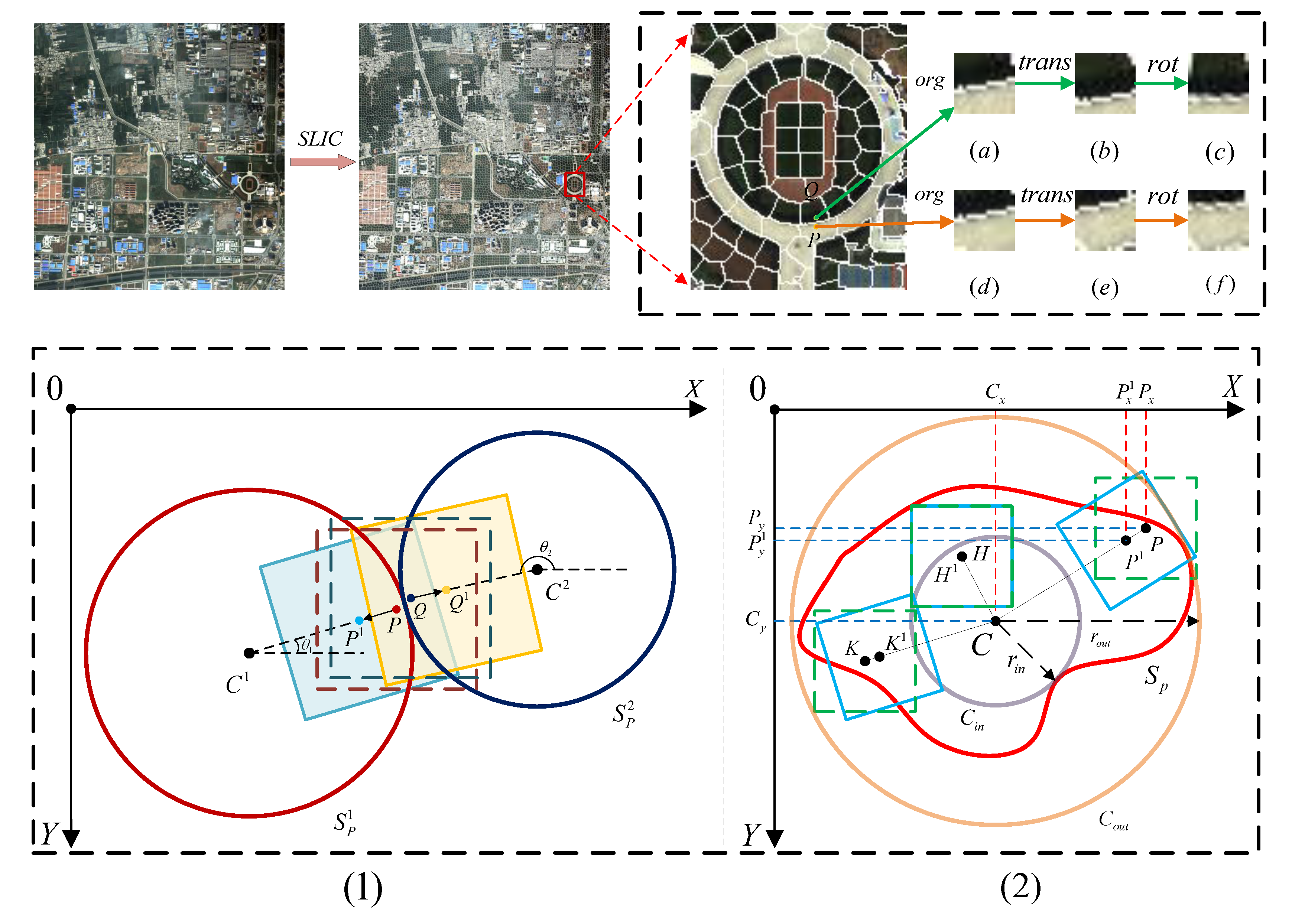
3.1. Adaptive Neighborhood Transfer Sampling Strategy

Deep learning (DL) is base on data-driven algorithms, which performance is directly affected by the quality of the training sample. Therefore, how to obtain effective samples is the first problem to be solved. As we know, remote sensing images are taken at high altitude, with large scenes and complex distribution of ground objects. In remote-sensing pixel-level classification tasks, the traditional sampling strategy is to extract pixel-centric (the pixel to be classified) orthogonal image patches. A patch provides neighbourhood information for its central pixel to determine the category of this central pixel. The traditional sampling strategy will obtain highly similar patches when pixels with very close Euclidean distances but belonging to different categories. Furthermore, due to the different distribution angles of ground objects, it is may not reasonable to set all patches with an orthogonal sampling angle to extract features.
Based on this, we put forward an adaptive neighbourhood transfer sampling strategy (ANTSS) that allows each patch to adaptively determine the neighbourhood range according to the homogeneity of the pixel to be classified. This strategy shifts the original patch centre (i.e., the pixel to be classified) to the homogeneous region to obtain more neighbourhood information with homogeneity to this pixel. It is expected to provide more positive feedback neighbourhood information for the classifier and makes patches obtained on the boundary of the two categories not repeat too much. The overall process of determining the neighbourhood range and sample angle of the patches can be referred to Figure 2(1). The main steps are in detail as follows:
(1) We should first determine the effective area of each homogeneous region in the image. Since the homogeneous region can be approximated as the aggregation of the same pixels category in the remote sensing image. Here, we choose a simple linear iterative clustering (SLIC) [35] superpixel algorithm to generate homogeneous region. The main reason is that SLIC as a local clustering algorithm, can aggregate a definite range of neighboUrhood pixels according to pixel characteristics. By performing SLIC-superpixel clustering, we determined the concrete distribution of homogeneous region in the image.
After obtaining the homogeneous region distribution in the image, we need to provide an indicative patch extraction for all pixels. Although the shape distribution of each homogeneous region is different, the centroid is the geometric centre of sectional graphics, which represents the relative position of the graphics in space. The relative relationship between the two centroids is also equivalent to the relative relationship between two homogeneous regions. When the pixels in the homogeneous area shift to the same centroid, while obtaining more homogeneous neighbourhood information, it also reduces the proportion of negative feedback information in the patch. Moreover, the sampling angle of the patch can be adaptively adjusted to capture more texture distribution information according to the spatial relationship between the centroid and the pixels. Assume that a superpixel contains N pixels, the centroid coordinates can be expressed as:
C x j = 1 n i = 1 n P x i C y j = 1 n i = 1 n P y i
where [ C x j , C y j ] is defined as centroid coordinates of the S p j homogenous region, and [ P x i , P y i ] is ith pixel coordinates in the same homogenous region.
(2) We next determine the definite neighbourhood range and sampling angle of each pixel according to the calculated centroid coordinates. As shown in the Figure 2(1), P and Q are two pixels with very close Euclidean distances but belonging to different categories, C 1 and C 2 are the centroid of the corresponding homogeneous regions respectively. With the transform of spatial relationships, we can calculate the new centre positions P 1 and Q 2 Furthermore, base on the relative position relationship between the pixel and the centroid, the sampling angle of the patch can be determined. Taking P as an example, the specific calculation of the neighbourhood transfer distance is as follows:
Firstly, for each pixel under the same homogeneous region, we need a measure of the spatial position relationship. Here we choose the Euclidean distance between the centroid and the pixel to represent the relative spatial position of a pixel in the homogeneous region. When the pixel is close to the edge of the homogeneous region, the Euclidean distance between the pixel and the centroid will increase, and the possibility of negative sampling will be greater. The Euclidean distance d i between the pixel P and the centroid C 1 is calculated as follows:
d i = ( P x C x 1 ) 2 + ( P y C y 1 ) 2
where [ P x , P y ] represent the coordinates of the pixel P, and [ C x 1 , C y 1 ] represent the coordinates of the centroid C 1 .
Secondly, to better distinguish pixels at different distances, we use two concentric circles to divide the superpixel into two regions. As shown in the Figure 2(2), one is to use the shortest distance between the edge pixel in the homogeneous region and the centroid as the radius r to generate concentric inscribed circles C i n . The other is to use the farthest distance between the edge pixel and the centroid as the radius R to generate a concentric circumcircle C o u t . When the pixel is located in C i n , there is more homogeneous neighbourhood information around the pixel, so there is no need to pass the neighbourhood range. On the contrary, when the pixel is located between C i n and C o u t , the neighbourhood range needs to transfer towards the centroid to capture more homogenous neighbourhood information to the original centre pixel P for feature extraction.
Finally, for pixels with different Euclidean distances, their neighborhood transfer distances should also be not the same. Furthermore, to maintain the diversity of samples, the neighborhood migration distance of pixels should not simply linearly increasing with Euclidean distance. This will constrain the sampling space, resulting in repeated sampling and generating redundant samples. Therefore, we introduce a two-dimensional Gaussian space and adaptively calculate the neighborhood transfer distance according to the Gaussian normal distribution. The neighbourhood transfer distance f ( x ) is calculated as follows:
f ( x ) = d i + 1 4 1 2 π exp ( 4 ( R d i ) + 1 R r ) 2 2 , r < d i < R 0 , o t h e r
where f ( x ) is obey standard statistics normal distribution function, d i + 1 4 represent the maximum distance of sample transfer, and 4 ( R d i ) + 1 R r is the Euclidean distance inverse proportional function. When the pixel d i is larger, the value of the inverse proportional function is smaller. Then the value of the Gaussian normal distribution is more extensive, and the corresponding neighbourhood transfer distance is more massive.
(3) Base on the transfer distance f x of the neighbourhood range and spatial angles θ 1 , we can calculate the new centre position P 1 of the patch. Then rotate clockwise θ 1 degree to extract the neighbourhood range according to the set patch size.
P x 1 = P x f ( d i ) × d i × sin θ P y 1 = P y f ( d i ) × d i × sin θ
where [ P x 1 , P y 1 ] is new center position coordinates.

3.2. Spatial Attention Module and Channel Attention Module

In the field of computer vision, the attention module has an excellent performance in enhancing image characteristics. Attention not only tells `where’ to focus but also tells `which’ to improve. In multi-resolution tasks, both MS data and PAN data have their individual data characteristics. MS data is rich in spectral information, and PAN data has a high spatial resolution. To improve the representation ability of feature, we use two different attention modules to highlight their respective feature representation. For PAN data, we use the spatial attention module to learn the `where’ of the spatial axis, to highlight the homogeneous regions of the pixels to be classified in the feature map. For MS data, we apply the channel attention module to learn the `which’ of the channel axis to focus on important features and suppress unnecessary features.
Based on this, we propose a local attention module (LSA-module) for PAN data and global channel attention module (GCA-module) for MS data. The local attention module (LSA-module) as shown in the Figure 3 and the global channel attention module (GCA-module) as shown in the Figure 4. The details of the attention modules are as follows:

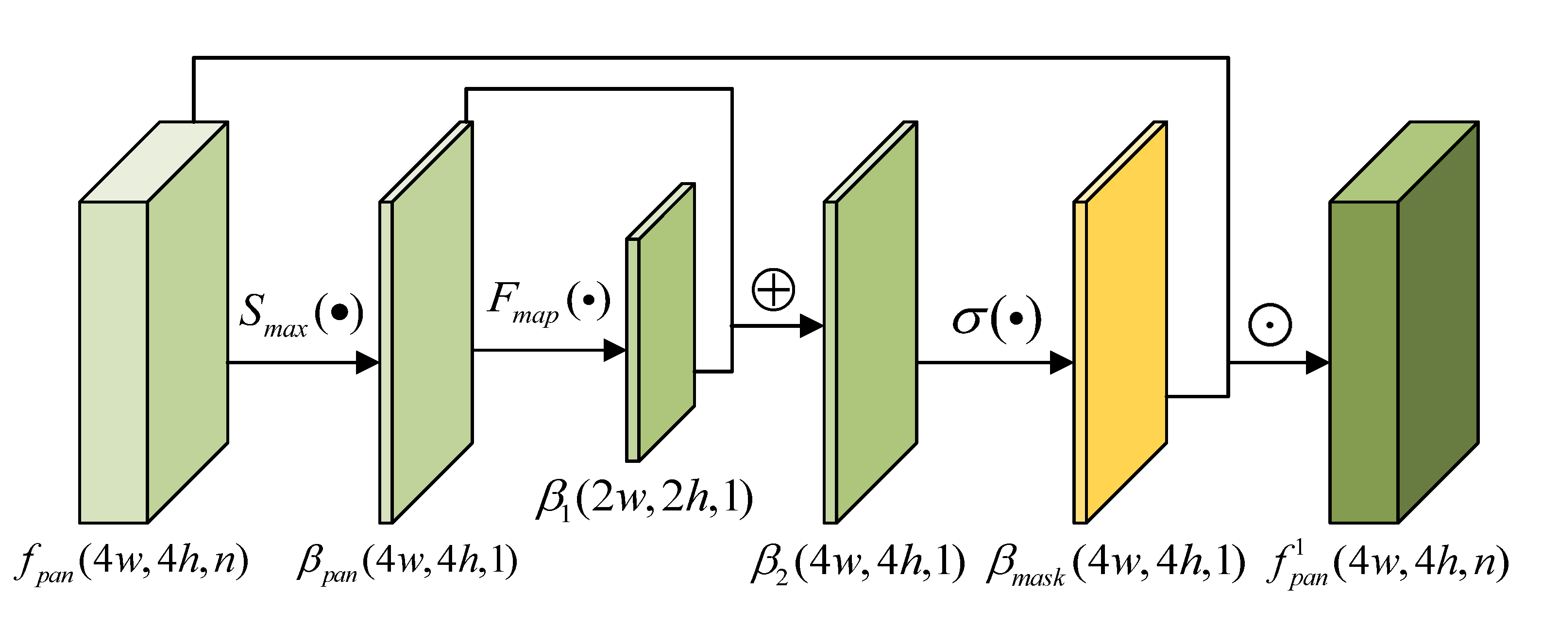
3.2.1. Spatial Attention Module

We produce a spatial attention mask by exploring the inter-spatial relationship of features. In the LSA-module, we capture the spatial context information of the feature map to focus on `where’ is an informative part. Our structure tends to combine a bottom-up feedforward operation and a top-down feedback operation into one feedforward operation. The bottom-up feedforward operation produces strong semantic information with low spatial resolution features, while the subsequent top-down operation combines high-resolution location information with strong semantic information to infer each pixel.
The detail process of the LSA-module is illustrated in Figure 3. Let the input of CA-module be f p a n R 4 W × 4 H × N , where 4 W , 4 H and N are width, height and channel dimension (i.e., number of filters). f p a n first do a spatial-wise maxpooling operation to aggregate the feature maps channel dimensions. Thus obtain a one-dimensional spatial-wise feature descriptors: β p a n R 4 W × 4 H × 1 .
β p a n = S m a x ( f p a n ) = 1 N i = 1 N f p a n i
where S m a x ( · ) is a maxpooling operation, which purpose is to preserve the feature important texture information and spatial position while reducing the channel dimension of the feature map. f p a n i represent the ith channel in the feature map.
We next apply a top-down feedforward operation to integrate spatial context information between features. In the spatial dimension of the patch, a global view of the image background can provide useful contextual information. However, not all background information is useful for improving the classification performance, and some meaningless background noise may even damage the classification accuracy. The network model is limited by the receptive field of the convolution kernel, and it is often unable to extract the global context information well. Therefore, we use the local spatial attention mechanism to enhance the useful local area in the feature to enhance the feature expression of each pixel. We use maxpooling to reduce the spatial resolution of the feature map, and then use convolution to build a nonlinear mapping to infer the relationship between pixels to generate a powerful semantic information mask β 1 .
β 1 = F m a p ( β p a n ) = C o n v 3 × 3 ( F m a x ( β p a n ) )
where F m a p ( · ) contains two nonlinear operations C o n v 3 × 3 ( · ) and F m a x ( · ) , which F m a x ( · ) is a maxpooling operation with a stride of 2, and C o n v 3 × 3 ( · ) is a convolution operation with a kernel size of 3. β 1 is a one-dimensional feature descriptors: β 1 R 2 W × 2 H × 1 .
Then, we use a top-down feedforward operation to combine high-level masks with high semantic information and low-level masks with high spatial resolution. Through convolution and pooling, we get a mask β 1 rich in semantic information. However, remote sensing images have different scales of features, and a single mask often fails to reflect all features well. When the feature target is too small, the convolved β 1 is often difficult to completely represent the target content. And some features have significant spectral information, and the shallow high-resolution features can complete the classification. Thus, we use the bilinear interpolation to increase the size of β 1 , and then add β p a n to obtain a high-resolution mask β 2 with strong semantic information.
β 2 = C o n c ( F i n ( β 1 ) , C o n v 1 × 1 ( β p a n ) )
where F i n ( · ) is a bilinear interpolation operations, and C o n c ( · ) represent the addition operation.
Subsequently, we use the activation function to get the weight distribution β m a s k of the spatial element, which value is distributed between [ 0 , 1 ] .
β m a s k = σ ( β 2 )
where σ ( · ) is sigmoid activation function, that role is to normalize the input.
Finally, we element-wise the spatial attention weight β m a s k with the original feature maps f p a n to obtain a spatial-enhanced feature maps f p a n 1 .
f p a n 1 = β m a s k f p a n

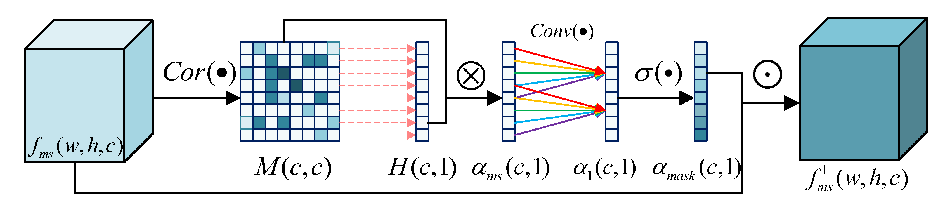
3.2.2. Channel Attention Module

As we all know, for different types of ground features, different channel response levels are different. Each channel map of feature is considered as a feature detector, channel attention focuses on `which’ is meaningful given an input image. By exploiting the inter-relationship between channel maps, we could emphasize interdependent feature maps and improve the feature representation of specific semantics. Therefore, we build a global channel attention module (GCA-module) to explore interdependencies between channels.
The structure of the global channel attention module is illustrated in Figure 4. Let the input of GCA-module be f m s R W × H × C , where W, H and C are width, height and channel dimension (i.e., number of filters), respectively. Precisely, we directly calculate the global channel correlation matrix M c c (c represents the row of the matrix and c represents the column of the matrix) from the original features f m s R W × H × C . We reshape f m s to two-dimensional matrix F c n (n is equal to w × h ), which represents spatial pixel intensity distribution between global channels. Subsequently, we perform a matrix multiplication between F c n and the transpose of F n c T to obtain a global channel correlation matrix M c c .
M = C o r ( f m s ) = F F T = R e ( f m s ) × R e ( f m s ) T
where C o r ( · ) is a matrix multiplication operation, R e ( · ) is reshape operation. Our purpose is to explore the dependence between the matrix F . Here, each element of the matrix F can be regarded as a class-specific response, and different semantic responses are associated with each other.
After obtaining the correlation matrix M c c of the feature maps, We average the elements in each row of the matrix M to obtain the channel correlation vector H C 1 . Each element in the vector H represents the spatial aggregation response of each channel in the feature map.
H i 1 = 1 c j = 1 c ( M i j )
where H i 1 is the value of the ith column of the vector H and M i j is the value of the ith column and jth row of the matrix M .
Subsequently, multiply the correlation M and the vector H to obtain the global channel correlation mask α m s . In the matrix multiplication operation, each row of M is element-wise multiplication by the entire column of H , which is equivalent to a global correlation comparison of all channels.
α m s = M × H
where α m s R C × 1 .
Next, we use fast 1-D convolution to generate the attention mask α 1 by exploring the dependencies between channels. Since the channels are related to each other, and the mask α m s includes specific global channel information. Therefore, we hope that there is a correspondence between the mask α m s and the attention mask α 1 . We did not use two fully-connected layers, but directly used convolution to build a non-linear mapping to obtain the attention mask. In this way, the dependency between channels is extracted while avoiding reducing the dimensionality of α m s .
α 1 = C o n v ( α )
where C o n v ( · ) is a convolution operation, and α 1 R C × 1
Then, we use the activation function to get the weight distribution α m a s k of the feature channel, which value is distributed between [ 0 , 1 ] .
α m a s k = σ ( α 1 )
where σ ( · ) is sigmoid activation function.
Finally, we element-wise the channel attention weight α m a s k with the original feature maps f m s to obtain a channel-enhanced feature maps f m s 1
f m s 1 = α m a s k f m s

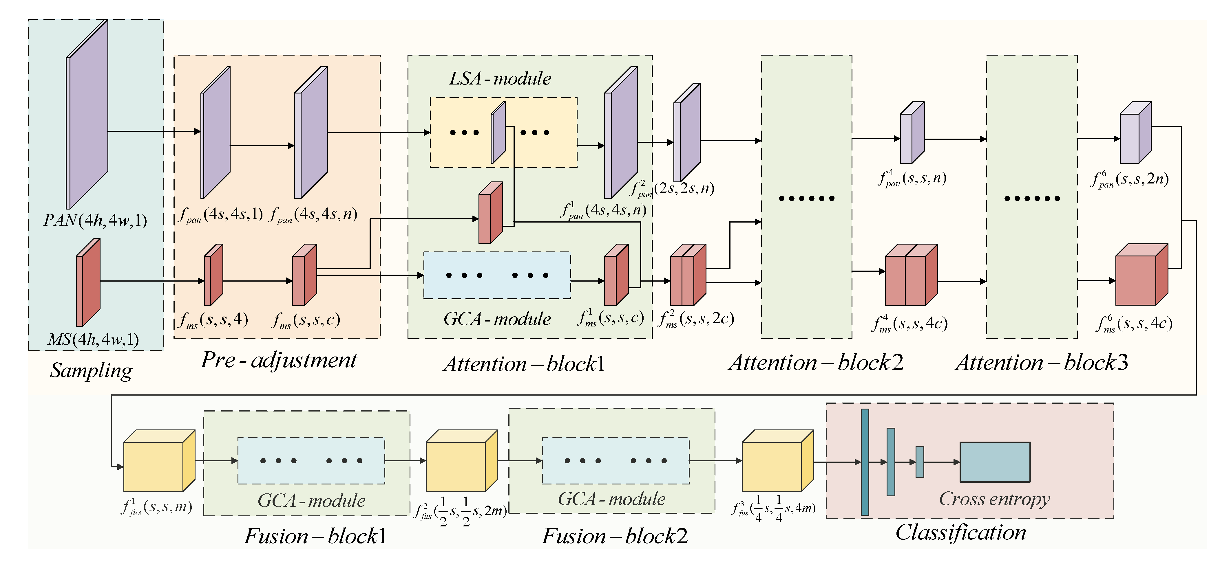
3.3. A Spatial-Channel Collaborative Attention Network (SCCA-Net)

In this part, based on the proposed above spatial attention module and channel attention module, we design a spatial spectrum collaborative network (SCCA-Net) for enhancement of multi-resolution classification. Since the complementary characteristics of multi-resolution data, we propose an attention collaboration network block. It aims to extract the characteristics of their respective data while alternate communicate the commonality information of PAN and MS. We multiply the spatial attention weight of the PAN branch with the original MS feature map element-wise to obtain a spatially enhanced MS feature map. Furthermore, in order to avoid the disappearance of the gradient caused by the network being too deep, we introduce the idea of Densenet [40], which concatenate the spatially enhanced MS feature map and the channel enhanced MS feature map. While transmitting the feature map of the shallow network, also brings a gradient cross-level flow. The proposed network framework as shown in Figure 5, and the details are as follows:
Data input: According to the above ANTSS Section 3.1 sampling strategy, we will obtain two different multi-resolution data patches. In this paper, the length (width) ratio of PAN and MS data is 4:1, so the PAN patch size is ( 128 , 128 , 1 ) and MS patch is ( 32 , 32 , 4 ) . All patches need to be normalized before entering the network.
The pre-adjustment: Before stacking the network modules, we must first perform pre-network adjustments (including convolution, batch normalization (BN) and rectified linear units (Relu)) on PAN and MS data to soften the input and improve the feature extraction effect of subsequent modules.
Stacking attention blocks: We combine the LSA-module of the PAN branch and the GCA-module of the MS branch to form attention-block and use three attention-block to form a module stacking layer, which is used as a feature extractor. In particular, we element-wise the spatial mask of the PAN branch with the original MS feature maps to obtain the spatially enhanced MS feature maps. Then, concatenate the channel enhancement MS feature map, and spatially enhancement MS feature map are used as the input of the next attention block. In this process, the two branch weights are not shared and independent of each other. Two attention modules collaborative to enhance the original information advantages of the respective image data types while further reducing the negative correlation differences of features. On one branch, the attention masks of the different modules capture different types of attention, and they are added to their respective features in the form of soft weights. The shallow mask mainly suppresses the unimportant information such as the background of the image, and as the network deepens, the mask gradually enhances the important information of interest.
Feature fusion and classification: To effectively fuse the features of these two branches, we performed the following operations for the output of the third attention block. In the third attention block, we no longer concatenate the previous layer features, but directly import the block as input. We concatenate the output f p a n 6 ( s , s , 2 n ) of the PAN branch and the output f m s 6 ( s , s , 4 c ) of the MS branch to obtain the fusion feature f f u s 1 ( s , s , m ) (m is equal to 4 c + 2 n ). In the in-depth convolution process, the network is more inclined to capture high-level semantic information, and they are more class-specific in the channel. So we only use GCA-module to enhance the channel of the feature map. Through several fully connected layers, the class probability of the pair of patches is finally estimated. In this paper, the cross-entropy error used as the ultimate loss function and defined as follows:
C = 1 N i = 1 n [ y i log ( y i 1 ) + ( 1 y i ) log ( 1 y i ) ]
where n denotes the batch size, y i is the label for the ith input pair, while y i 1 is the class probability for the ith input pair. We train this end-to-end network using the stochastic gradient descent (SGD) strategy.

4. Experimental Study

In this section, the proposed method will be evaluated on the dataset of different areas, and we also compare our method with several state-of-art algorithms. The experimental results and analysis as follow:

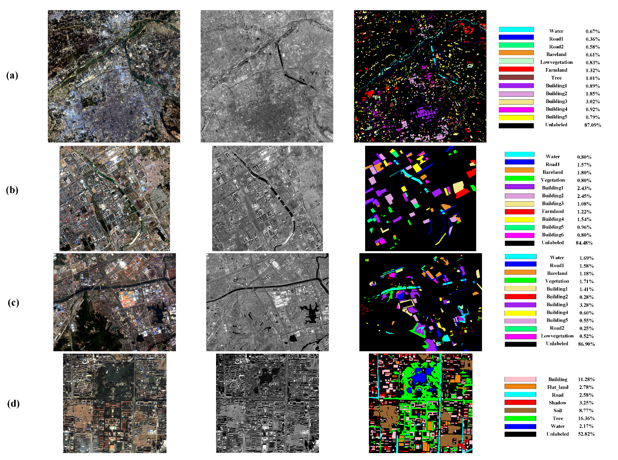
4.1. Data Description

In this part, we use four datasets to verify the robustness and effectiveness of the proposed method. Each dataset of multiresolution in the experiment contains a pair of corresponding PAN and MS data. The three first data sets (Figure 6a–c) are obtained by the GaoFen I sensor; the last data set (Figure 6d) is obtained by the QuickBird sensor.
Xi’an Level 1A image set:Figure 6a shows the Level 1A data, which has been calibrated and radiometrically corrected: processed include data analysis, homogenization radiation correction, denoising, MTFC, CCD stitching, band registration, etc. It was acquired on 29 August 2015, in Xi’an, China. The MS component consists of 4548 × 4541 × 4 pixels with a spatial resolution of 8 m, while the PAN component consists of 18,192 × 18,164 pixels with a spatial resolution of 2 m. The data was divided into 12 categories, which includes five kinds of buildings, two kinds of roads, lowvegetation, tree, bareland, farmland, and water.
Huhehaote Level 1A image set:Figure 6b is Level 1A data, which was acquired in Huhehaote China on 23 May 2015. The MS component consists of 2001 × 2101 × 4 pixels with a spatial resolution of 4m, while the PAN component consists of 8004 × 8404 pixels with a spatial resolution of 1 m. The scene was divided into 11 categories, which includes six kinds of buildings, road, tree, bareland, farmland, and water.
Nanjing Level 1A image set:Figure 6c is Level 1A data, this one acquired in Nanjing China on 21 April 2015. The MS component consists of 2000 × 2500 × 4 pixels with a spatial resolution of 4 m, while the PAN component consists of 8000 × 10,000 pixels with a spatial resolution of 1 m. This data was divided into 11 categories, which includes five kinds of buildings, two kinds of vegetation, two kinds of roads, bareland, and water.
Xi’an Ubarn image set:Figure 6d shows the Xi’an Urban area, which acquired in Xi’an, China, on 30 May 2008. The MS component consists of 800 × 830 × 4 pixels with a spatial resolution of 2.44 m, while the PAN component consists of 3200 × 3320 pixels with a spatial resolution of 0.61 m. This scene was divided into 7 categories, which consist of building, road, tree, soil, flatland, water, and shadow. Flat land represents all kinds of land except soil.
The experiments in this paper are running on Workstation with RTX1080Ti 11GB GPU and 128GB RAM under Ubuntu 16.04 LTS. The proposed network is trained on PyTorch.

4.2. Experimental Setup

For evaluating the classification performance, the metrics including overall accuracy (OA), average accuracy (AA), and kappa statistic (Kappa) are calculated to perform quantitative analysis. Since the PAN data is often tricky to mark, the groundtruth image is corresponding to its MS data pixel by pixel. Therefore, we first intercept the MS sample patch from the MS image by ANTSS, and map the centre point of this patch to the corresponding PAN data; then we intercept the PAN sample patch with it as the centre. Corresponding to the flow chart of Figure 6, the detailed hyper-parameters of the proposed SCCA-Net are shown in Table 1. To avoid similar samples input to the test network affecting the accuracy of the final classification result, the test sample patch whose IoU ratio to the training sample patch is greater than 0.8 is not input to the network for testing. The input size of the PAN and MS patches are ( 4 S × 4 S ; 1 ) and ( S × S ; 4 ) , respectively.
In the training of the network, we randomly select 5% of the labeled data of each category as the training dataset, and the remaining samples are used as the test dataset. The initial learn rate is 0.001 , the weight decay is 0.0005, the iteration number is 50,000, and the batch size is 64. In order to ensure that the proposed framework is sufficiently variable, we code 10 times for different random training samples, and take the average result as the final result for each metric.

4.3. The Comparison and Analysis of Hyper-Parameters

In this section, we make a detailed comparison and analysis of the hyperparameters in this paper: the selection of kernel size k in GCA-module. Except for different hyperparameters selected, each set of data is trained and tested applying an SCCA-net with the same other parameters.

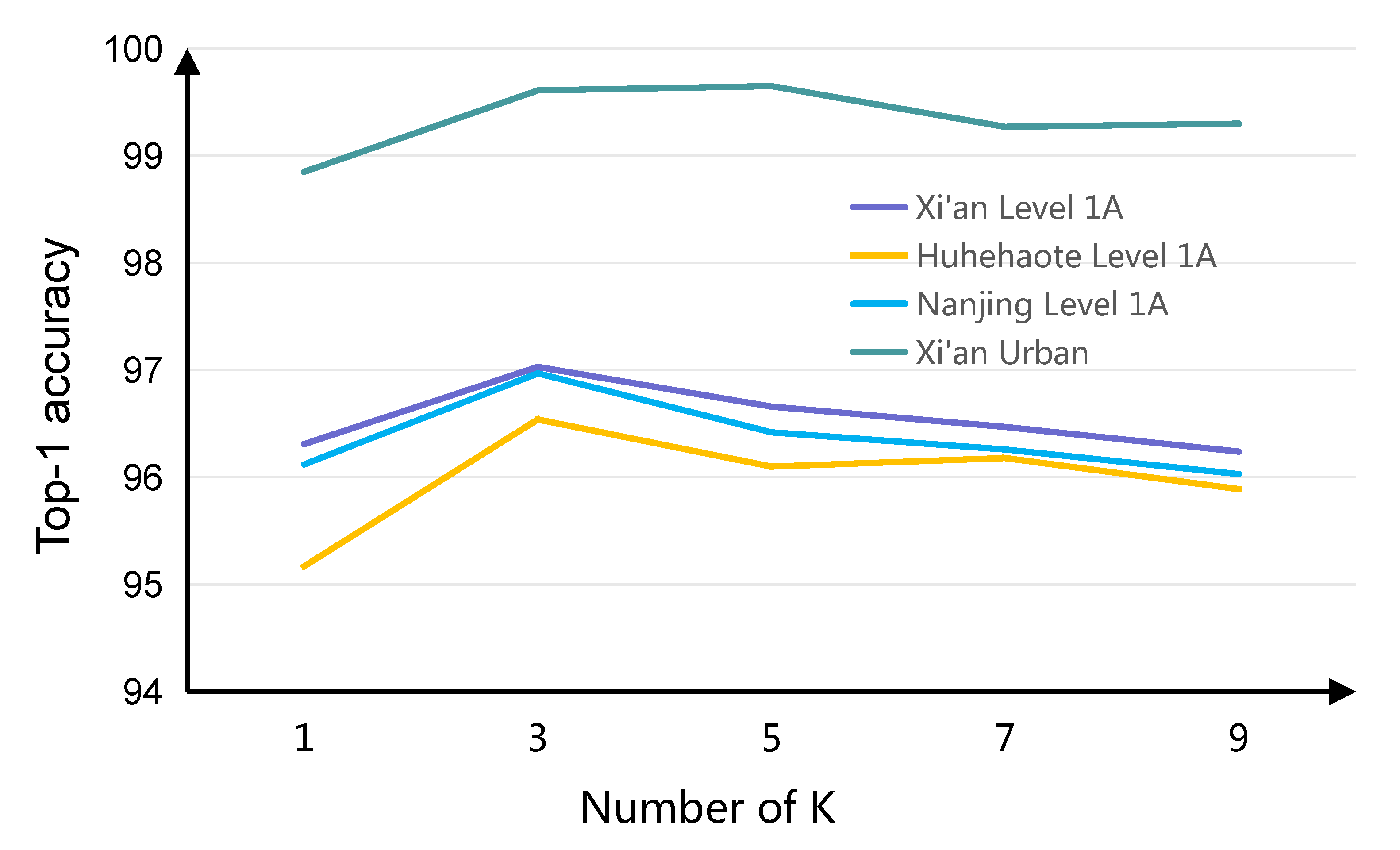
Effect of Kernel Size Selection

As shown in Figure 4, our GCA-module involves a parameter k, which represents a kernel size of 1 D convolution. In this part, we mainly evaluate its effect on our GCA-module and validate the effectiveness of the proposed selection of kernel size. To this end, we employ SCCA-net as a backbone network and train them with our GCA-module by setting k be from 1 to 9. The results are illustrated in Figure 7, from it we have the following observations.
First, in the quantitative comparison of different data sets, when the size of the convolution kernel k = 3 , the best classification result can be obtained. For the convolution kernel size k, it represents the number of interactive channels in the feature map. Generally, it can be expected that larger-sized channels are suitable for remote interactions, while smaller-sized channels are good for short-term interactions. Since our network has a relatively shallow number of layers, the number of channels in the feature map is relatively small. However, when k = 1 , it is equivalent to independently learning the weight of each channel. This shows that attention weights require to consider the relationship between channels appropriately. Moreover, when k = 5 , 7 , 9 , although the relationship between channels is considered, the result is not the highest. This shows that the number of interaction channels and the effectiveness of the attention model does not increase linearly. The excessive number of interactive channels will be mixed with some negative channel information, resulting in the attention weight value is not optimal. Finally, when k = 3 , there is a direct correspondence between channels and masks, and smaller-sized channels are prefer to use smaller-sized convolution kernels. Therefore, we set the size of the convolution kernel to k = 3 .

4.4. Performance of The Proposed Sampling Strategy and Attention Module

In this section, taking Xi’an urban images as an example, we do a detailed comparison and analysis of the proposed adaptive neighbourhood transfer sampling strategy (ANTSS) and two kinds of attention models, respectively.

4.4.1. Validation of the Proposed Adaptive Neighborhood Transfer Sampling Strategy (ANTSS) Performance

In this part, we verify the effectiveness of the ANTSS strategy by comparing several sampling strategies in remote sensing classification tasks. ANTSS adaptively selects the most appropriate neighbourhood patch base on the surrounding pixel distribution and adjusts the angle of the patch according to the shape of the object to be classified. Except for the ACO-SS adaptive determines the size of a patch (patch size S respectively are 12, 16 and 24), the rest of the sampling strategy patches size S is 32. A N T S S * use the ANTSS method to transfer the sample neighbourhood, but use an orthogonal sliding window to crop all patches evenly. The proportion of training samples selected by these methods is the same. All sampling strategies use Resnet18 [41] as the backbone network, and network-related hyper-parameters are also the same for fair.
The results of the experiment are shown in Table 2; it can be seen that our ANTSS obtained the highest classification result. Comparing A N T S S * with Pixel-Centric and SML-SS, all the results of A N T S S * are better than these two methods, which means that the neighbourhood information range should be different for different categories. By transfer the neighbourhood range of the sample to the homogeneous region, we have obtained patches that are more helpful for network classification. Moreover, comparing A N T S S * with ANTSS, we can see that the classification results of all categories have been improved, which shows that our adaptive sampling angle can obtain complete texture structure information to improve the feature expression ability. Therefore, it is unreasonable for the traditional central sampling strategy in remote sensing images to use orthogonal sampling angles for all samples. Moreover, the patch neighbourhood information may be mixed with many other categories of information when the neighbourhood range is fixed, which will have a negative effect on determining the category of the centre pixel. Since our ANTSS sampling strategy can effectively avoid the above problems, thus improving the overall classification performance.

4.4.2. Validation of the Proposed Spatial-Channel Cooperative Attention Network (SCCA-Net) Performance

In this part, we want to verify whether the proposed modules are more suitable for our remote-sensing image classification task. Thus, we use several different attention models (SE-module [30] and CBAM-module [37]) to compare our proposed attention models (respectively are LSA-Net, GCA-Net, SCCA-Net). Here, the sampling strategy of these network models is ANTSS, and each pair of comparison models has the same hyper-parameters and iteration times. The Xi’an Urban data set is used as the input for these network models, each attention model all uses a dual-branch network, and the same stacked attention model is used on both branches. In the SCCA-Net, the PAN image of Xi’an Urban data set is used as the input of the LSA-model and the MS image of Xi’an Urban data set is used as the input of GCA-Net.
The experimental comparison results are shown in the Table 3, from which we have the following observation results. Firstly, our LSA-Net achieves higher classification results than CBAM-Net and SE-Net. Because the training samples of remote sensing images usually have some differences in the same category, and there are also some similarities between different categories. When the network tends to be deeper, the ordinary attention network will easily fall into an optimal local state, which will cause the network to be unstable after training. Secondly, comparing our GCA-Net and LSA-Net, the former obtained better classification results. This show that in deep convolution, the network extracts high-level semantic information features and the channel response between different categories is more important. Besides, the SCCA-Net obtained the best classification results, indicating that different network modules should be designed for different data to extract more robust feature representations. And the information flow between features can prevent the network from falling into a local optimum, from better integrating the characteristics of their respective features. Experiments show that our SCCA-Net can extract more stable features from complex remote sensing data, and the collaborative work between modules can bring about the flow of gradient information and enhance the classification performance of the network.

4.5. Performance of Experimental Results and Comparison Algorithm

In this part, we will compare various methods on four data sets to verify the effectiveness of our proposed method in detail.

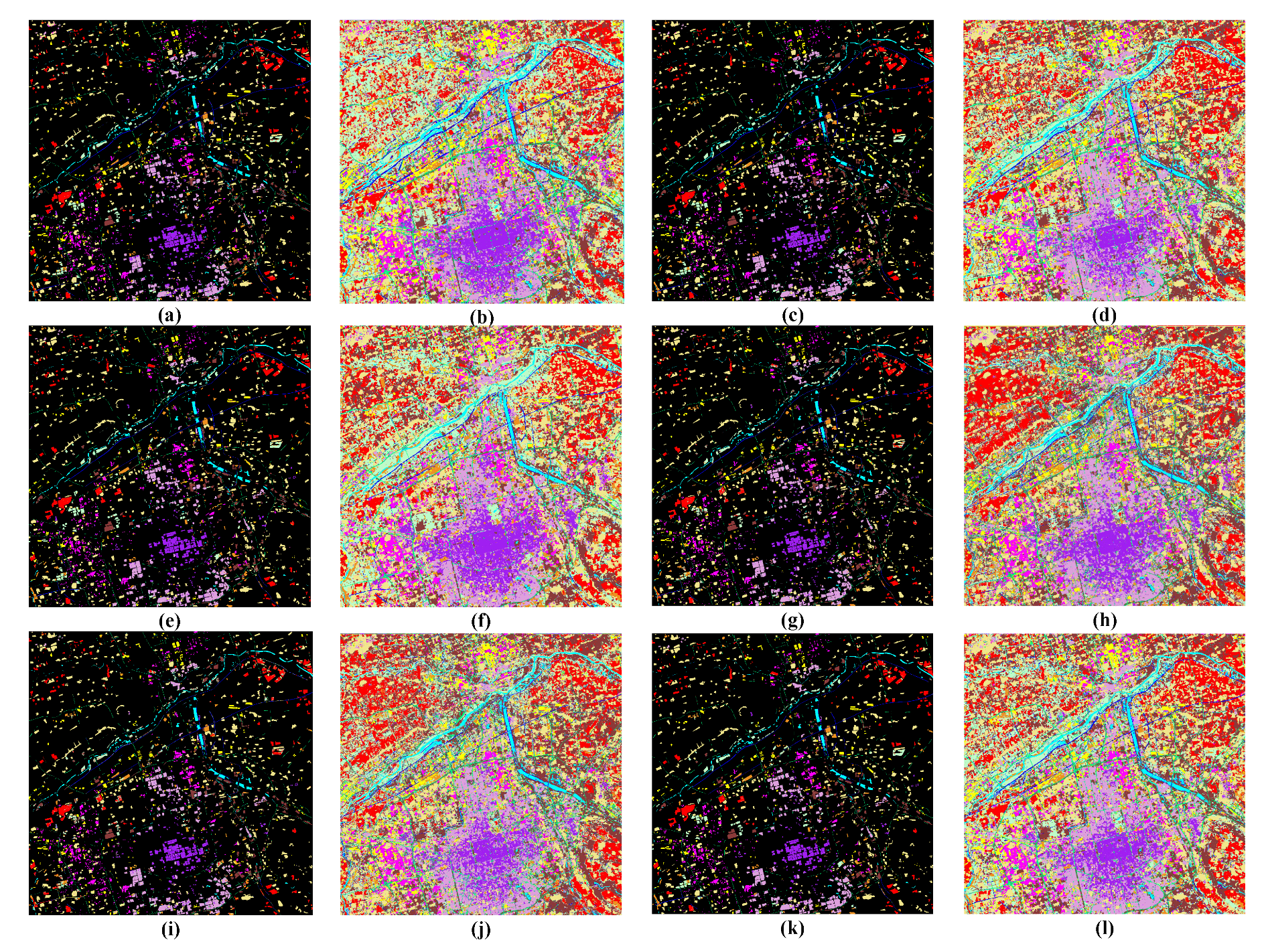
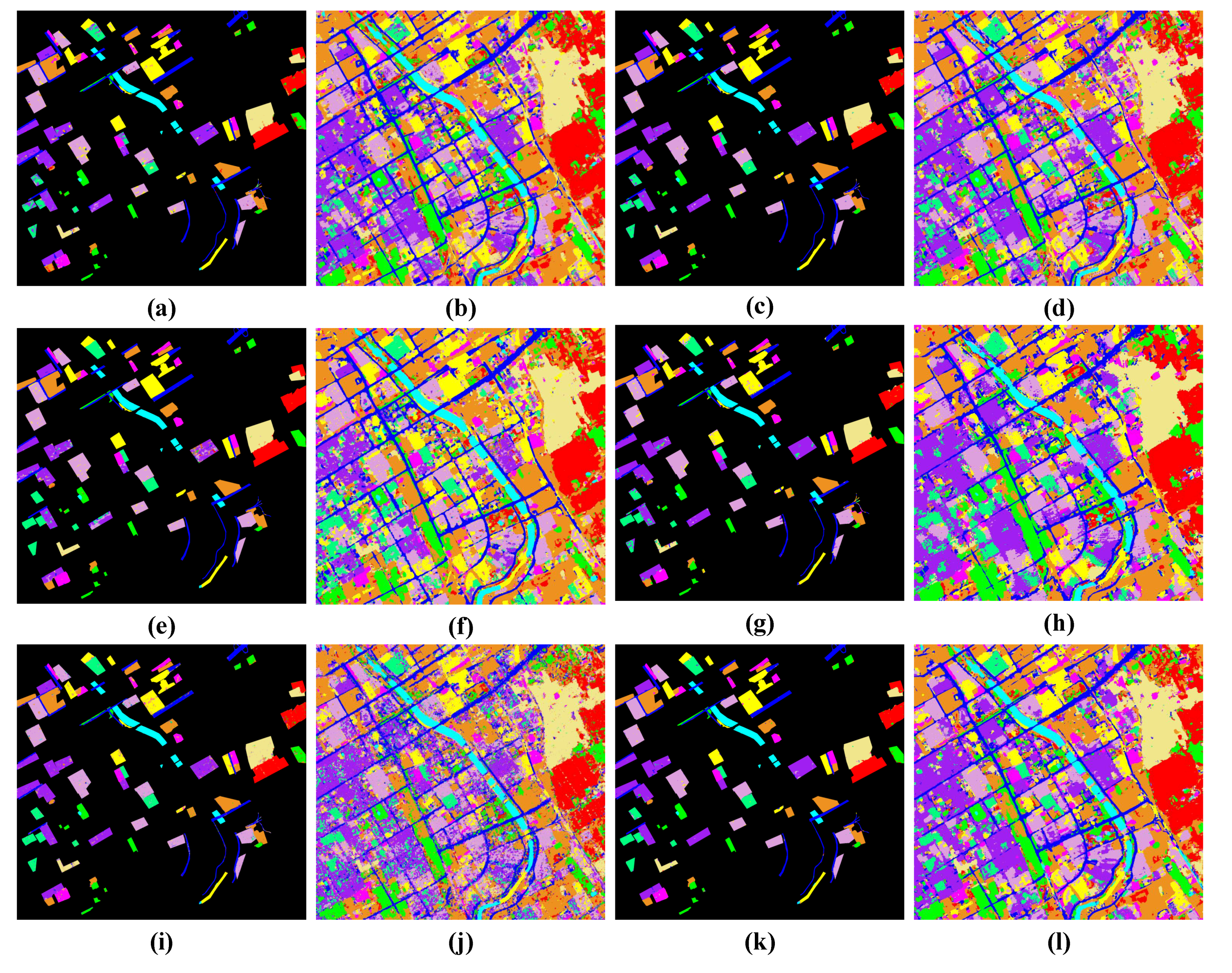
4.5.1. Experimental Results with Xi’an Level 1A Images

In this part, taking Xi’an Level 1A Images as an example, we compare the various methods to verify the effectiveness of the proposed method in detail. Three state-of-the-art methods, namely DMIL [24], SML-CNN [25] and DBFA-net [27] in this paper are used as the compared methods. These methods are multiresolution classification methods based on neural network, which is reasonable and suitable to use them as the comparison algorithms. For these networks, we follow the experimental setup in their respective papers to achieve their best results. Moreover, we also designed 3 sets of ablation experiments combining the current excellent classification modules, namely: Pixel-Centric+SE-Net(Res18) [30], ANTSS+SE-Net(Res18), and ANTSS+CBAM(Res18) [37]. Here, Pixel-Centric+SE-Net and ANTSS+SE-Net in Table 4 denotes that SE-model extract the features of the PAN branch and the MS branch, and then concatenate the features of two branches for final classification. Besides, Pixel-Centric+SE-Net uses the traditional pixel-centric sampling strategy, and ANTSS+SE-Net uses our proposed ANTSS sampling strategy. ANTSS+CBAM-Net [37] is used SA-module to extract features in the PAN branch while use CA-module to extract features in the MS branch, which also uses the ANTSS sampling strategy. We compared our SCCA-Net with other methods; the specific analysis is as follows:
Compare Pixel-Centric+SE-Net with ANTSS+SE-net: AS shown in Table 4 and Figure 8. Based on the same backbone network, the ANTSS+SE-net obtain higher results than SE-Net. After adding our proposed ANTSS sampling strategy, most of the category accuracy has been improved. In particular, the accuracy of c 2 ( r o a d 1 ) , c 4 ( b a r e l a n d ) and c 5 ( l o w v e g e t a t i o n ) are significantly improved, from 88.41 % to 90.76 % , 86.70 % to 89.33 % , and 81.55 % to 88.62 % respectively. It can be seen from the groundtruth map that c 2 and c 4 are widely distributed and intertwined between each category, so the original neighbourhood range does not reflect the true nature of this category well. The results indicate that our ANTSS is not only feasible on the specific SCCA-Net, but also can be promoted in other networks.
And it is noted that due to the limited performance of the SE-module, sampling strategy does not raise too much accuracy, some categories obtained lower accuracy. Compared with the other results in Table 4, the overall OA, AA, and Kappa of the above two methods are not high. So we also need some network modules with better performance to classify.
Compare SCCA-Net with ANTSS+SE-Net: From the Table 4, our SCCA-Net gets the highest classification results in most categories, and the overall accuracy (OA), Average accuracy (AA) and Kappa of SCCA-Net are also the highest. This shows that SCCA-Net combines the advantages of ANTSS and attention module so that the classification accuracy can be further improved. However, the accuracy of c 7 ( t r e e ) and c 11 ( b u i l d i n g 4 ) in SCCA-Net is lower than that of ANSS+SE-Net. Specifically, the accuracy of c 7 ( t r e e ) and c 11 ( b u i l d i n g 4 ) is slightly lower 0.06 and 0.07 than ANSS+SE-Net, respective. Further inspection of the classification results of c 7 reveals that the network divides part of c 5 into c 7 . We analyze that because the spectral characteristics of these categories are very similar, and the spatial scale differences are relatively small. It is difficult for the network to distinguish them completely. Moreover, the accuracy of c 11 in our classification network is not relatively high, which may be because our network suppresses the water category too much in the process of channel enhancement, resulting in low classification accuracy.
Compare SCCA-Net with ANTSS+CBAM: As above, the S C C A N E T * obtained better results than CBAM(Res18) based on the same central pixel sampling strategy, the accuracy of most categories has improved significantly. Our SCCA-Net makes up for the shortcomings of the general attention network that is easy to fall into local optimum, and enhances the feature extraction ability to deal with complex remote-sensing patches. The accuracies of some categories (e.g., c 5 ( l o w v e g e t a t i o n ) , c 8 ( b u i l d i n g 1 ) , c 10 ( b u i l d i n g 3 ) ) have been improved much. Since their information is more comfortable confuse with other categories, and our SCCA-Net uses different attention modules to extract the respective data characteristics of multi-resolution. The spatial texture feature of the category is extracted through the LSA-module and mapped to the MS feature maps, which enhances its spatial characteristics, and uses GCA-module to adjust the response of the feature channel to complete the classification of difficult categories.
However, the accuracy of our SCCA-Net in c 7 ( t r e e ) , and c 11 ( b u i l d i n g 4 ) is slightly lower than that of ANSS+CBAM. Through the analysis of the confusion matrix of the classification results, we found that the classification accuracy of c 7 ( t r e e ) decreased mainly because our network misclassified some c 5 ( l o w v e g e t a t i o n ) as c 7 ( t r e e ) . Since the category difference between c 5 ( l o w v e g e t a t i o n ) and c 7 ( t r e e ) in multiresolution images is minimal, they are distinguished mainly by geographic location information and some spatial texture information. Therefore, when we use the PAN feature spatial detail information to enhance the spatial resolution of MS feature while improving the network’s ability to discriminate c 5 ( l o w v e g e t a t i o n ) as c 7 ( t r e e ) , it also produces a part of misclassified samples.
Compare SCCA-Net with DBFA-Net, DMIL, and SML-CNN: Moreover, our SCCA-Net is also superior to the results of the three state-of-the-art remote sensing image classification methods. DMIL respectively uses the stacked-DCNN model to extract the features of PAN data, and the stacked-Auto-Encoders (SAE) model extracts the features of MS data. However, the network is relatively shallow, and it is not able to adequately extract robust and significant feature representations when dealing with remote sensing data with complex characteristics. Therefore, the accuracy of most categories of DMIL is lower than SCCA-Net. SML-CNN first use the six local regions of the superpixel (four corner regions, an original region and a central region) as input, and then designed six-multiple CNN model for feature extraction, finally, it used the multi-layer Auto-Encodering to fuse the output of the network for classification. Compared with DMIL, it obtained better results, but it has very low accuracy at categories with less training samples (e.g., c 2 ( r o a d 1 ) : 0.815 % , c 3 ( r o a d 2 ) : 0.8668 % , c 4 ( b a r e l a n d ) : 0.8789 % , c 5 ( l o w v e g e t a t i o n ) : 0.8334 % ).
It is worth noting that ACO-SS + DBAF-Net first adaptively generates multi-scale training samples according to the texture structure of the image, and then uses spatial and channel attention mechanisms to extract the features of PAN and MS data respectively. Therefore, the classification accuracy of most ACO-SS + DBAF-Net categories is higher than that of DMIL and SML-CNN. However, due to the external differences between MS and PAN data, the features extracted by DBAF-Net are also very different. Therefore, the overall classification performance of the network is lower than our SCCA-Net.
Test time: Finally, we also compared the efficiency of all algorithms, such as DMIL, SML-CNN and ACO-SS + DBAF-Net. Among these algorithms, our running time is the longest. Because we use a attention mechanism to enhance feature representation, the network structure is more complicated. At the beginning of the design of the network, our goal was to use different attention module for different remote sensing data. Moreover, we added branches of information flow between the two attention modules to reduce the differences between the two while maintaining the unique characteristics of each data. It does improve not only the accuracy of network classification but also brings additional computational costs. So our next research goal is how to maintain high precision while further improving the efficiency of the algorithm.

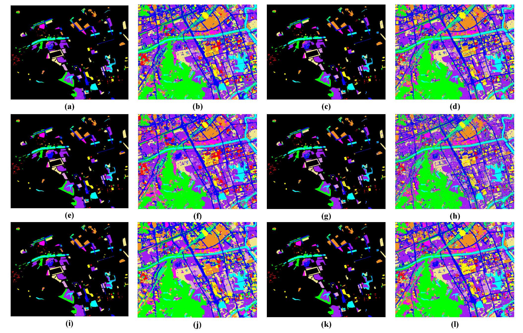
4.5.2. Experimental Results with Huhehaote Level 1A Images

The comparison of the results of the other three data set is similar to the Xi’an Level 1A data set. For the three datasets, the SCCA-Net obtains the highest AA, OA, and Kappa.
The quantitative and qualitative results of the Huhehaote 1A level data set are shown in the Table 5 and Figure 9. By comparison, the classification results of c 2 ( r o a d 1 ) , c 3 ( b a r l a n d ) and c 6 ( b u i l d i n g 2 ) are relatively poor, and they belong to the more difficult categories in all categories. This result indicates that we need to improve the discrimination ability of these class features through precise strategies. Through the analysis of the groundtruth map and the classification result, it can be seen that c 2 ( r o a d 1 ) is widely distributed and interleaved with multiple categories, and it is easy to misclassify it according to the ordinary method. The experimental results of our method show that ANTSS and SCCA-Net all achieved more significant improvements in these categories. The accuracy of most categories of SCCA-Net has reached the highest level, but some categories are slightly less effective. We think it may be due to data fusion that the discriminative power of the features of these categories is reduced, thereby reducing the classification results.

4.5.3. Experimental Results with Nanjing Level 1A Images

For the Nanjing 1A level data set, the quantitative and qualitative results are shown in Table 6 and Figure 10. It can be seen that c 2 ( r o a d 1 ) and c 11 ( l o w v e g e t a t i o n ) belong to the more difficult category in all categories. Since c 2 ( r o a d 1 ) is widely distributed and adjacent to other categories, if a traditional sampling strategy is used, it is easy to obtain patches with different categories but the similar neighbourhood. And the category features of c 2 ( r o a d 1 ) and c 10 ( r o a d 2 ) are very similar, which makes the network easy to fall into the local optimum and lead to misclassification.
c 11 ( l o w v e g e t a t i o n ) is similar to c 4 ( v e g e t a t i o n ) in terms of spectrum information and geographic shape, when the discriminative performance of the network is poor, they cannot be distinguished well. We use ANTSS to generate the training data set, which can well separate some pixels that generate confusing samples. Moreover, our SCCA-Net combining the channel and spatial attention mechanism can enhance the extracted feature representation and improve the discriminative representation of the network. Our methods obtained the highest OA, AA, KAPPA in most categories and the highest classification accuracy in most categories. But we did not achieve the highest accuracy on c 3 ( b a r e l a n d ) and c 10 ( r o a d 2 ) , which may be because the spectral characteristics of these categories are pronounced, and the additional spatial detail information leads to network performance decline.

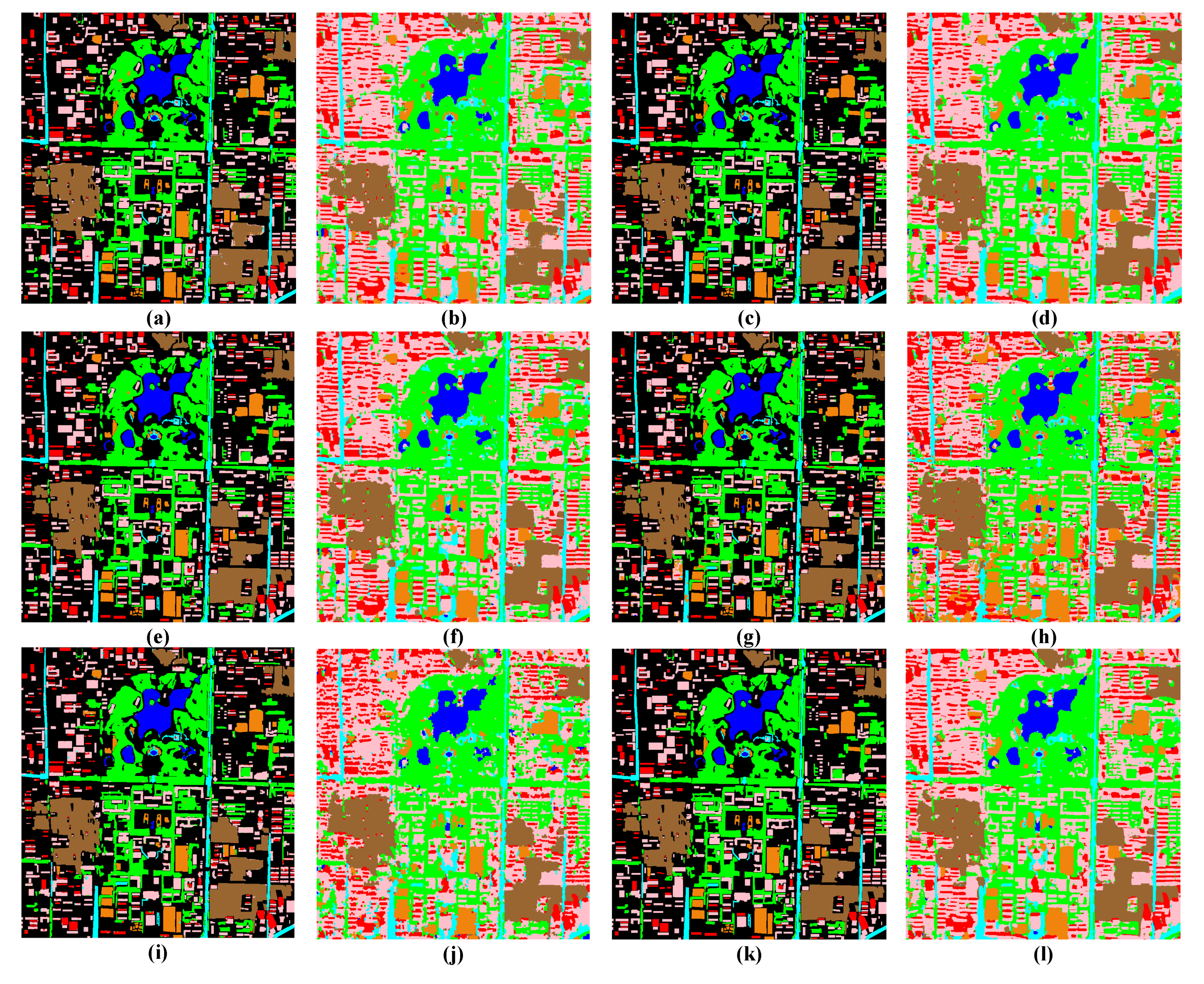
4.5.4. Experimental Results with Xi’an Urban Images

For the Xi’an Urban data set, the quantitative and qualitative results are shown in Table 7 and Figure 11. Because the data itself is small, ACO-SS+DBAF-Net has almost reached the upper-performance limit, so our SCCA-NET improvement is not apparent. Among all categories, the classification results of c 3 ( r o a d ) and c 7 ( w a t e r ) are slightly lower than other categories. Through ground facts, we can know that c 3 ( r o a d ) is widely distributed and irregular in shape, and often closely connected with c 1 ( b u i l d i n g ) . Our ANTSS Sampling strategy can solve the problem of unequal sample distribution, which can improve the recognition ability of the network through SCCA-Net. Finally, because there are fewer categories of Xi’an features, and each category is relatively simple compared with the above data set, our SCCA-Net has obtained high experimental results. Although our method did not get the highest result on c 7 ( w a t e r ) , the accuracy of the highest A C O S S + D B A F N e t is 99.61 % , the difference not big.

5. Conclusions

In this paper, we propose spatial-channel collaborative attention enhance network for multiresolution remote sensing image classification. And experiments on several data sets have verified the effectiveness of our ANTSS strategy, LSA-module and GCA-module. However, our algorithm still has some shortcomings. Firstly, before using ANTSS to generate training samples, we use the SLic-superpixel algorithm to perform superpixel segmentation. Therefore, our method needs a good superpixel algorithm to segment multiresolution data. Secondly, due to the SCCA-Net is more complicated, the computational complexity is relatively high, so the running time is longer. In the future, we will focus on how to build a more concise channel-spatial collaborative attention module while maintaining the same accuracy to improve the efficiency of multi-resolution remote sensing image classification.

Author Contributions

Validation, J.S. and L.J.; writing—original draft preparation, J.Z.; writing—review and editing, H.Z.; Funding acquisition, W.M.; Supervision, W.M., Y.W. and B.H. All authors have read and agreed to the published version of the manuscript.

Funding

This work was supported in part by the State Key Program of National Natural Science of China under Grant 61836009, in part by the National Natural Science Foundation of China under Grant U1701267, Grant 61671350 and Grant 62006179, in part by the China Postdoctoral Science Special funded project under Grant 2020T130492, and in part by the China Postdoctoral Science Foundation funded project under Grant 2019M663634.

Conflicts of Interest

The authors declare no conflict of interest.

References

  1. Nunez, J.; Otazu, X.; Fors, O.; Prades, A.; Pala, V.; Arbiol, R. Multiresolution-based image fusion with additive wavelet decomposition. IEEE Trans. Geosci. Remote Sens. 1999, 37, 1204–1211. [Google Scholar] [CrossRef] [Green Version]
  2. Jia, X.; Richards, J.A. Cluster-space representation for hyperspectral data classification. IEEE Trans. Geosci. Remote Sens. 2002, 40, 593–598. [Google Scholar]
  3. Li, S.; Kang, X.; Fang, L.; Hu, J.; Yin, H. Pixel-level image fusion:A survey of the state of the art. Inf. Fusion 2017, 33, 100–112. [Google Scholar] [CrossRef]
  4. Israa, A.; Javier, M.; Miguel, V.; Rafael, M.; Katsaggelos, A. A survey of classical methods and new trends in pansharpening of multispectral images. EURASIP J. Adv. Signal Process. 2011, 1, 79. [Google Scholar]
  5. Giuseppe, M.; Davide, C.; Luisa, V.; Giuseppe, S. Pansharpening by Convolutional Neural Networks. Remote Sens. 2016, 8, 594. [Google Scholar]
  6. Zhong, J.; Yang, B.; Huang, G.; Zhong, F.; Chen, Z. Remote Sensing Image Fusion with Convolutional Neural Network. Sens. Imaging 2016, 17, 10. [Google Scholar] [CrossRef]
  7. Liu, Y.; Chen, X.; Wang, Z.; Wang, Z.; Jane, K.W.; Wang, X. Deep learning for pixel-level image fusion: Recent advances and future prospects. Inf. Fusion 2018, 42, 158–173. [Google Scholar] [CrossRef]
  8. Shackelford, A.K.; Davis, C.H. A hierarchical fuzzy classification approach for high-resolution multispectral data over urban areas. IEEE Trans. Geosci. Remote Sens. 2003, 41, 1920–1932. [Google Scholar] [CrossRef] [Green Version]
  9. Moser, G.; Serpico, S.B. Joint classification of panchromatic and multispectral images by multiresolution fusion through Markov random fields and graph cuts. In Proceedings of the 2011 17th International Conference on Digital Signal Processing (DSP), Corfu, Greece, 6–8 July 2011; pp. 1–8. [Google Scholar]
  10. Pham, M.; Mercier, G.; Michel, J. Pointwise Graph-Based Local Texture Characterization for Very High Resolution Multispectral Image Classification. IEEE J. Sel. Top. Appl. Earth Obs. Remote Sens. 2015, 8, 1962–1973. [Google Scholar] [CrossRef]
  11. Moser, G.; De Giorgi, A.; Serpico, S.B. Multiresolution Supervised Classification of Panchromatic and Multispectral Images by Markov Random Fields and Graph Cuts. IEEE Trans. Geosci. Remote Sens. 2016, 54, 5054–5070. [Google Scholar] [CrossRef]
  12. Zhang, J.; Li, T.; Lu, X.; Cheng, Z. Semantic Classification of High-Resolution Remote-Sensing Images Based on Mid-level Features. IEEE J. Sel. Top. Appl. Earth Obs. Remote Sens. 2016, 9, 2343–2353. [Google Scholar] [CrossRef]
  13. Mao, T.; Tang, H.; Wu, J.; Jiang, W.; He, S.; Shu, Y. A Generalized Metaphor of Chinese Restaurant Franchise to Fusing Both Panchromatic and Multispectral Images for Unsupervised Classification. IEEE Trans. Geosci. Remote Sens. 2016, 54, 4594–4604. [Google Scholar] [CrossRef]
  14. Thomas, C.; Ranchin, T.; Wald, L.; Chanussot, J. Synthesis of Multispectral Images to High Spatial Resolution: A Critical Review of Fusion Methods Based on Remote Sensing Physics. IEEE Trans. Geosci. Remote Sens. 2008, 46, 1301–1312. [Google Scholar] [CrossRef] [Green Version]
  15. Tu, T.; Su, S.; Shyu, H.; Huang, P.S. A new look at IHS-like image fusion methods. Inf. Fusion 2001, 2, 177–186. [Google Scholar] [CrossRef]
  16. Tu, T.; Huang, P.S.; Hung, C.; Chang, C. A fast intensity-hue-saturation fusion technique with spectral adjustment for IKONOS imagery. IEEE Geosci. Remote Sens. Lett. 2004, 1, 309–312. [Google Scholar] [CrossRef]
  17. Wold, S.; Esbensen, K.H.; Geladi, P. Principal Component Analysis. Chemom. Intell. Lab. Syst. 1987, 2, 37–52. [Google Scholar] [CrossRef]
  18. Candes Emmanuel, J.; Li, X.; Ma, Y.; Wright, J. Robust principal component analysis. J. ACM 2011, 58, 11. [Google Scholar]
  19. Huang, F.; Yan, L. Study on the Hyperspectral Image Fusion Based on the Gram Schmidt Improved Algorithm. Inf. Technol. J. 2013, 12, 6694–6701. [Google Scholar] [CrossRef]
  20. Pradhan, P.S.; King, R.L.; Younan, N.H.; Holcomb, D.W. Estimation of the Number of Decomposition Levels for a Wavelet-Based Multiresolution Multisensor Image Fusion. IEEE Trans. Geosci. Remote Sens. 2006, 44, 3674–3686. [Google Scholar] [CrossRef]
  21. Zheng, S.; Shi, W.; Liu, J.; Tian, J. Remote Sensing Image Fusion Using Multiscale Mapped LS-SVM. IEEE Trans. Geosci. Remote Sens. 2008, 46, 1313–1322. [Google Scholar] [CrossRef]
  22. Yang, S.; Wang, M.; Jiao, L. Fusion of multispectral and panchromatic images based on support value transform and adaptive principal component analysis. Inf. Fusion 2012, 13, 177–184. [Google Scholar] [CrossRef]
  23. Vivone, G.; Alparone, L.; Chanussot, J.; Dalla Mura, M.; Garzelli, A.; Licciardi, G.; Restaino, R.; Wald, L. A Critical Comparison Among Pansharpening Algorithms. IEEE Trans. Geosci. Remote Sens. 2015, 53, 2565–2586. [Google Scholar] [CrossRef]
  24. Liu, X.; Jiao, L.; Zhao, J.; Zhao, J.; Zhang, D.; Liu, F.; Yang, S.; Tang, X. Deep Multiple Instance Learning-Based Spatial Spectral Classification for PAN and MS Imagery. IEEE Trans. Geosci. Remote Sens. 2018, 56, 461–473. [Google Scholar] [CrossRef]
  25. Zhao, W.; Jiao, L.; Ma, W.; Zhao, J.; Zhao, J.; Liu, H.; Cao, X.; Yang, S. Superpixel-Based Multiple Local CNN for Panchromatic and Multispectral Image Classification. IEEE Trans. Geosci. Remote Sens. 2017, 55, 4141–4156. [Google Scholar] [CrossRef]
  26. Ma, W.; Zhang, J.; Wu, Y.; Jiao, L.; Zhu, H.; Zhao, W. A Novel Two-Step Registration Method for Remote Sensing Images Based on Deep and Local Features. IEEE Trans. Geosci. Remote Sens. 2019, 57, 4834–4843. [Google Scholar] [CrossRef]
  27. Zhu, H.; Ma, W.; Li, L.; Jiao, L.; Yang, S.; Hou, B. A Dual Branch Attention fusion deep network for multiresolution remote Sensing image classification. Inf. Fusion 2020, 58, 116–131. [Google Scholar] [CrossRef]
  28. Bergado, J.R.; Persello, C.; Stein, A. Recurrent Multiresolution Convolutional Networks for VHR Image Classification. IEEE Trans. Geosci. Remote Sens. 2018, 56, 6361–6374. [Google Scholar] [CrossRef] [Green Version]
  29. Zhu, H.; Jiao, L.; Ma, W.; Liu, F.; Zhao, W. A Novel Neural Network for Remote Sensing Image Matching. IEEE Trans. Neural Netw. Learn. Syst. 2019, 30, 2853–2865. [Google Scholar] [CrossRef]
  30. Hu, J.; Shen, L.; Albanie, S.; Sun, G.; Wu, E. Squeeze and Excitation Networks. IEEE Trans. Pattern Anal. Mach. Intell. 2019, 42, 2011–2023. [Google Scholar] [CrossRef] [Green Version]
  31. Carrasco, M. Visual attention: The past 25 years. Vis. Res. 2011, 51, 1484–1525. [Google Scholar] [CrossRef] [Green Version]
  32. Itti, L.; Koch, C.; Niebur, E. A model of saliency-based visual attention for rapid scene analysis. IEEE Trans. Pattern Anal. Mach. Intell. 1998, 20, 1254–1259. [Google Scholar] [CrossRef] [Green Version]
  33. Beuth, F.; Hamker, F.H. A mechanistic cortical microcircuit of attention for amplification, normalization and suppression. Vis. Res. 2015, 116, 241–257. [Google Scholar] [CrossRef] [PubMed]
  34. Gao, Z.; Xie, J.; Wang, Q.; Li, P. Global Second Order Pooling Convolutional Networks. In Proceedings of the IEEE/CVF Conference on Computer Vision and Pattern Recognition (CVPR), Long Beach, CA, USA, 15–21 June 2019. [Google Scholar]
  35. Wang, Q.; Wu, B.; Zhu, P.; Li, P.; Zuo, W.; Hu, Q. ECA-Net: Efficient Channel Attention for Deep Convolutional Neural Networks. In Proceedings of the IEEE/CVF Conference on Computer Vision and Pattern Recognition (CVPR), Seattle, WA, USA, 14–19 June 2020. [Google Scholar]
  36. Roy, A.G.; Navab, N.; Wachinger, C. Recalibrating Fully Convolutional Networks With Spatial and Channel `Squeeze and Excitation’ Blocks. IEEE Trans. Med. Imaging 2019, 38, 540–549. [Google Scholar] [CrossRef] [PubMed]
  37. Woo, S.; Park, J.; Lee, J.-Y.; Kweon, I.S. CBAM: Convolutional Block Attention Module. In Proceedings of the European Conference on Computer Vision (ECCV), Munich, Germany, 8–14 September 2018. [Google Scholar]
  38. Fu, J.; Liu, J.; Tian, H.; Li, Y.; Bao, Y.; Fang, Z.; Lu, H. Dual Attention Network for Scene Segmentation. In Proceedings of the IEEE Conference on Computer Vision and Pattern Recognition, Long Beach, CA, USA, 15–21 June 2019; pp. 3146–3154. [Google Scholar]
  39. Huang, Z.; Wang, X.; Huang, L.; Huang, C.; Wei, Y.; Liu, W. CCNet: Criss-Cross Attention for Semantic Segmentation. In Proceedings of the IEEE International Conference on Computer Vision, Seoul, Korea, 27 October–3 November 2019; pp. 603–612. [Google Scholar]
  40. Huang, G.; Liu, Z.; Der Maaten, L.V.; Weinberger, K.Q. Densely Connected Convolutional Networks. In Proceedings of the IEEE Conference On Computer Vision And Pattern Recognition, Honolulu, HI, USA, 21–26 July 2017; pp. 2261–2269. [Google Scholar]
  41. He, K.; Zhang, X.; Ren, S.; Sun, J. Deep Residual Learning for Image Recognition. In Proceedings of the IEEE Conference on Computer Vision and Pattern Recognition (CVPR), Las Vegas, NV, USA, 27–30 June 2016. [Google Scholar]
Figure 1. The overall process of traditional pixel-central sample sampling. (a,c) are sample patches that are similar but do not belong to the same category; (b,d) are sample patches of the same category but with closer Euclidean distance.
Remotesensing 13 00106 g001
Figure 2. The overall process of determining the neighbourhood pixels and centre position of the patches. (1) The mathematical analysis of the concrete sampling process is shown below the figure. The lower left sub-figure (1) represent sampling process of two pixels located in different superpixel regions; the lower right sub-figure (2) represents sample sampling process of pixels at different locations in the same superpixel region. (2) The actual sampling results are shown in the upper right: (a) and (d) are the original sampling results; (b) and (e) are the sample patches after neighborhood transfer, (c) and (f) are the sample patch after the sampling angle is rotated
Remotesensing 13 00106 g002
Figure 3. The proposed spatial attention module (LSA-module) for PAN branch.
Remotesensing 13 00106 g003
Figure 4. The proposed channel attention module (GCA-module) for MS branch.
Remotesensing 13 00106 g004
Figure 5. The proposed a spatial-channel attention enhancement network (SCCA-Net) for multiresolution classification. The network is divided into four parts: the first is to pre-adjust the feature map; the second is to stack attention blocks for feature extraction; then the feature fusion is performed; and finally the three fully-connection layers is used for classification.
Remotesensing 13 00106 g005
Figure 6. First column: MS image. Second column: PAN images (The PAN image is reduced to the same size as their MS image for a more convenient display). Third column: Ground truth image. Last column: The class labels corresponding to the ground truth image. (a) Xi’an Level 1A image set ( 4548 × 4541 pixels). (b) Huhehaote Level 1A image set ( 2001 × 2101 pixels). (c) Nanjing Level 1A image set ( 2000 × 2500 pixels). (d) Xi’an Ubarn image set ( 800 × 830 pixels).
Remotesensing 13 00106 g006
Figure 7. Results of our GCA-module with various numbers of k using SCCA-net as backbone network.
Remotesensing 13 00106 g007
Figure 8. Classification maps of different methods on the Xi’an Level 1A Images ( 4548 × 4541 ), each method has two classification maps: one is image with ground truth, while the other is overall image. (a,b) Pixel-Centric+SE-Net(Res18). (c,d) ANTSS+SE-Net(Res18). (e,f) ACO-SS+DBAF-Net. (g,h) DMIL. (i,j) SML-CNN. (k,l) ANTSS+SCCA-Net.
Remotesensing 13 00106 g008
Figure 9. Classification maps of different methods on the Hohhot Level 1A Images( 2001 × 2101 ), each method has two classification maps: one is image with ground truth, while the other is overall image. (a,b) Pixel-Centric+SE-Net(Res18). (c,d) ANTSS+SE-Net(Res18). (e,f) ACO-SS+DBAF-Net. (g,h) DMIL. (i,j) SML-CNN (k,l) ANTSS+SCCA-Net.
Remotesensing 13 00106 g009
Figure 10. Classification maps of different methods on the Nanjing Level 1A Images ( 2000 × 2500 ), each method has two classification maps: one is image with ground truth, while the other is overall image. (a,b) Pixel-Centric+SE-Net(Res18). (c,d) ANTSS+SE-Net(Res18). (e,f) ACO-SS+DBAF-Net. (g,h) DMIL. (i,j) SML-CNN (k,l) ANTSS+SCCA-Net.
Remotesensing 13 00106 g010
Figure 11. Classification maps of different methods on the Xi’an Urban area Images( 800 × 830 ), each method has two classification maps: one is image with ground truth, while the other is overall image. (a,b) Pixel-Centric+SE-Net(Res18). (c,d) ANSS+SE-Net(Res18). (e,f) ACO-SS+DBAF-Net. (g,h) DMIL. (i,j) SML-CNN (k,l) ANSS+DBSCCA-Net.
Remotesensing 13 00106 g011
Table 1. The Hyper-Parameters of Each Network Layer.
TypesInputPANMSOutput
P r e j u s t 4 S × 4 S , 1
( S × S , 4 )
C o n v 2 d , 5 × 5 B a t c h N o r m R e l u C o n v 2 d , 3 × 3 B a t c h N o r m R e l u 4 S × 4 S , 3
( S × S , 6 )
A t t e n t i o n b l o c k 1 4 S × 4 S , 3
( S × S , 6 )
M a x p o o l C o n v 2 d , 5 × 5 B a t c h N o r m R e l u
I n t e r p o l a t i o n C o n v 2 d , 1 × 1 B a t c h N o r m R e l u
C o n v 2 d , 3 × 3 B a t c h N o r m R e l u C o n v 2 d , 3 × 3 B a t c h N o r m A v g p o o l C o n v 1 d , 3 S i g m o i d 2 S × 2 S , 6
( S × S , 12 )
A t t e n t i o n b l o c k 2 2 S × 2 S , 6
( S × S , 12 )
M a x p o o l C o n v 2 d , 3 × 3 B a t c h N o r m R e l u
I n t e r p o l a t i o n C o n v 2 d , 1 × 1 B a t c h N o r m R e l u
C o n v 2 d , 3 × 3 B a t c h N o r m R e l u C o n v 2 d , 3 × 3 B a t c h N o r m A v g p o o l C o n v 1 d , 3 S i g m o i d S × S , 12
( S × S , 24 )
A t t e n t i o n b l o c k 3 S × S , 12
( S × S , 24 )
M a x p o o l C o n v 2 d , 3 × 3 B a t c h N o r m R e l u
I n t e r p o l a t i o n C o n v 2 d , 1 × 1 B a t c h N o r m R e l u
C o n v 2 d , 3 × 3 B a t c h N o r m R e l u C o n v 2 d , 3 × 3 B a t c h N o r m A v g p o o l C o n v 1 d , 3 S i g m o i d S × S , 24
( S × S , 48 )
f u s i o n b l o c k 1 S × S , 72 C o n v 2 d , 3 × 3 B a t c h N o r m R e l u C o n v 2 d , 3 × 3 B a t c h N o r m A v g p o o l C o n v 1 d , 3 S i g m o i d × 2 1 2 S × 1 2 S , 72
f u s i o n b l o c k 2 1 2 S × 1 2 S , 72 C o n v 2 d , 3 × 3 B a t c h N o r m R e l u C o n v 2 d , 3 × 3 B a t c h N o r m A v g p o o l C o n v 1 d , 3 S i g m o i d × 2 1 4 S × 1 4 S , 144
A v g 1 4 S × 1 4 S , 144 A v g p o o l 1 × 1 , 144
f c 1 × 1 , 144 f c , [ 144 , 36 , c l a s s ] 1 × 1 , c l a s s
Table 2. Quantitative comparison over different sampling strategies on the Xi’an Urban image data.
Sampling StrategiesPixel-Centric
( S = 32 )
SML-SS
( S = 32 )
ACO-SS
( S = 12 , 16 , 24 )
ANTSS
( S = 32 )
ANTSS *
( S = 32 )
c 1 ( % ) 97.7395.7698.1199.3699.45
c 2 ( % ) 97.6297.2999.9199.4799.32
c 3 ( % ) 96.7494.2599.9099.1498.74
c 4 ( % ) 95.8895.7399.2999.4499.07
c 5 ( % ) 97.9898.4299.8199.8399.65
c 6 ( % ) 97.8597.6698.4399.6699.52
c 7 ( % ) 98.5496.3599.6199.6499.46
OA(%)97.6796.7399.0899.5699.41
AA(%)97.4896.2199.2999.5199.32
Kappa(%)97.2894.1298.8899.4499.28
Table 3. Quantitative comparison over different network models on the Xi’an Urban image data.
Network ModelsSE-NetCBAM-NetLSA-NetGCA-NetSCCA-Net
c 1 ( % ) 96.8399.1699.5099.5599.50
c 2 ( % ) 94.9499.4799.7199.7699.74
c 3 ( % ) 97.9498.9098.6598.6799.13
c 4 ( % ) 93.4299.1398.8398.9099.08
c 5 ( % ) 99.9099.6399.7999.7299.89
c 6 ( % ) 98.8699.4799.1499.1599.69
c 7 ( % ) 98.0198.4099.7799.5599.64
OA(%)97.8599.1699.3899.4199.61
AA(%)97.1399.1099.3599.2899.52
Kappa(%)97.2299.0399.3399.3699.50
Table 4. Quantitative Classification Results of Xi’an Level 1A Images.
MethodsPixel-Centric
(S = 32)
+SE-Net
ANTSS
(S = 32)
+SE-Net
ANTSS
(S = 32)
+CBAM-Net
ACO-SS
(S = 12, 16, 24)
+DBFA-Net
DMIL
(S = 16)
SML-CNN
(S = 16)
ANTSS
(S = 32)
+SCCA-Net
c 1 ( % ) 97.2397.2797.9298.7897.9497.9098.75
c 2 ( % ) 88.4190.7694.8898.4183.8681.597.01
c 3 ( % ) 92.3393.7495.9792.9285.4886.6896.33
c 4 ( % ) 86.7089.3393.3192.0476.9387.8997.78
c 5 ( % ) 81.6588.6288.8185.3176.1083.3489.56
c 6 ( % ) 91.3893.7895.8999.0890.4993.6699.28
c 7 ( % ) 96.0696.3796.7597.8588.8394.6096.30
c 8 ( % ) 85.4788.6691.2494.5291.0090.4299.79
c 9 ( % ) 90.8092.7394.1398.6196.3392.9496.55
c 10 ( % ) 97.6697.2397.9095.7697.8395.9699.53
c 11 ( % ) 95.2196.8698.1196.8496.8298.1096.79
c 12 ( % ) 89.0492.7193.4998.1292.3592.9596.74
OA(%)92.8994.3295.3595.9191.9192.8897.13
AA(%)92.0993.7194.5195.6989.5091.3496.53
Kappa(%)91.7193.1594.1794.7090.8291.9296.74
Test Time(s)600.70721.41857.161125.78900.56702.962061.31
Table 5. Quantitative Classification Results of Huhehaote Level 1A Images.
MethodsPixel-Centric+
(S = 32)
+SE-Net
ANSS+
(S = 32)
+SE-Net
ANTSS
(S = 32)
+CBAM-Net
ACO-SS+
(S = 12, 16, 24)
+DBFA-Net
DMIL
(S = 16)
SML-CNN
(S = 16)
ANSS+
(S = 32)
+SCCA-Net
c 1 ( % ) 98.4899.3499.2899.2195.6199.1898.84
c 2 ( % ) 88.1190.3694.0292.2491.2591.0494.72
c 3 ( % ) 91.3194.4596.0194.0492.5393.1495.37
c 4 ( % ) 92.1295.1395.4397.6092.3591.5996.24
c 5 ( % ) 90.4194.2894.8299.9791.9192.7498.09
c 6 ( % ) 94.6995.9895.6491.1492.4094.7296.12
c 7 ( % ) 90.8895.7697.1796.1197.2191.3798.84
c 8 ( % ) 89.6189.4296.9796.4298.3095.4896.57
c 9 ( % ) 88.7092.6995.1492.6092.1593.4197.63
c 10 ( % ) 94.4993.8195.4792.2784.0992.9996.93
c 11 ( % ) 93.4594.3793.7397.5192.3888.8298.11
OA(%)92.2094.7895.6294.8092.6093.2096.80
AA(%)91.8994.3295.7995.3892.7493.1396.95
Kappa(%)90.6393.8795.0994.1891.7292.3996.42
Test Time(s)198.76226.04362.02454.21322.94346.86386.28
Table 6. Quantitative Classification Results of Nanjing Level 1A Images.
MethodsPixel-Centric+
(S = 32)
+SE-Net
ANSS+
(S = 32)
+SE-Net
ANTSS
(S = 32)
+CBAM-Net
ACO-SS+
(S = 12, 16, 24)
+DBFA-Net
DMIL
(S = 16)
SML-CNN
(S = 16)
ANSS+
(S = 32)
+SCCA-Net
c 1 ( % ) 95.9596.8096.8596.9796.1095.8796.01
c 2 ( % ) 78.8093.4092.8593.6987.2289.3594.92
c 3 ( % ) 87.2596.8597.8998.3694.1695.9796.53
c 4 ( % ) 95.2094.8196.2397.1690.7694.7398.00
c 5 ( % ) 89.3497.3697.0796.2894.8095.9696.82
c 6 ( % ) 89.5599.4199.3198.1297.7796.7799.55
c 7 ( % ) 94.4294.8994.1797.5990.6593.6098.58
c 8 ( % ) 85.0998.2597.7599.1695.5693.3698.09
c 9 ( % ) 95.1996.6196.9495.3692.7891.6598.30
c 10 ( % ) 93.1797.0196.9797.0292.7691.9896.69
c 11 ( % ) 87.4890.7292.7775.2377.8786.3693.54
OA(%)91.9895.6195.5795.7191.6093.6497.16
AA(%)90.5595.1896.2694.9991.8693.2496.94
Kappa(%)90.7194.9194.8695.0390.2492.6296.71
Test Time(s)187.16178.55425.04306.15339.95226.03395.64
Table 7. Quantitative Classification Results of Xi’an Urban area Images.
MethodsPixel-Centric+
(S = 32)
+SE-Net
ANSS+
(S = 32)
+SE-Net
ANTSS
(S = 32)
+CBAM-Net
ACO-SS+
(S = 12, 16, 24)
+DBFA-Net
DMIL
(S = 16)
SML-CNN
(S = 16)
ANSS+
(S = 32)
+SCCA-Net
c 1 ( % ) 96.1198.3298.8698.1193.6892.7798.68
c 2 ( % ) 92.2096.1299.3699.9195.1595.2999.97
c 3 ( % ) 94.4698.4698.8799.9096.4392.2599.61
c 4 ( % ) 91.1396.8197.8899.2993.4792.2799.38
c 5 ( % ) 99.6299.6799.7599.8198.5998.8199.88
c 6 ( % ) 98.8099.0799.0198.4396.6597.6699.70
c 7 ( % ) 98.8298.8799.7199.6198.6797.3599.58
OA(%)96.2598.6299.0899.0896.0995.2099.65
AA(%)95.8898.1999.0699.2994.8995.5899.51
Kappa(%)96.1198.2398.8198.8893.2194.6999.58
Test Time(s)113.8077.5494.26364.79263.19165.57324.25
Publisher’s Note: MDPI stays neutral with regard to jurisdictional claims in published maps and institutional affiliations.

