Relation-Constrained 3D Reconstruction of Buildings in Metropolitan Areas from Photogrammetric Point Clouds


1
Department of Land Surveying and Geo-informatics, The Hong Kong Polytechnic University, Hung Hom, Kowloon, Hong Kong
2
School of Geospatial Engineering and Science, Sun Yat-Sen University, Zhuhai 519082, China
*
Author to whom correspondence should be addressed.
Remote Sens. 2021, 13(1), 129; https://0-doi-org.brum.beds.ac.uk/10.3390/rs13010129
Submission received: 25 November 2020
/
Revised: 25 December 2020
/
Accepted: 28 December 2020
/
Published: 1 January 2021
(This article belongs to the Special Issue 3D Urban Scene Reconstruction Using Photogrammetry and Remote Sensing)
Abstract
:The complexity and variety of buildings and the defects of point cloud data are the main challenges faced by 3D urban reconstruction from point clouds, especially in metropolitan areas. In this paper, we developed a method that embeds multiple relations into a procedural modelling process for the automatic 3D reconstruction of buildings from photogrammetric point clouds. First, a hybrid tree of constructive solid geometry and boundary representation (CSG-BRep) was built to decompose the building bounding space into multiple polyhedral cells based on geometric-relation constraints. The cells that approximate the shapes of buildings were then selected based on topological-relation constraints and geometric building models were generated using a reconstructing CSG-BRep tree. Finally, different parts of buildings were retrieved from the CSG-BRep trees, and specific surface types were recognized to convert the building models into the City Geography Markup Language (CityGML) format. The point clouds of 105 buildings in a metropolitan area in Hong Kong were used to evaluate the performance of the proposed method. Compared with two existing methods, the proposed method performed the best in terms of robustness, regularity, and topological correctness. The CityGML building models enriched with semantic information were also compared with the manually digitized ground truth, and the high level of consistency between the results suggested that the produced models will be useful in smart city applications.
1. Introduction
Point clouds, either from laser scanning or photogrammetric processing, are the main data sources for three-dimensional (3D) urban reconstruction. Aerial laser scanning (ALS) point clouds can provide accurate 3D information about large-scale scenes and have therefore been widely used for 3D building reconstruction in urban areas [1,2,3]. However, vertical surfaces (such as building façades) are often completely missing from the ALS data, resulting in a huge loss of vertical information. Therefore, many previous studies focused only on the reconstruction of building rooftops [4,5] and produced 2.5D building models [6,7]. In contrast, oblique photogrammetry can produce dense image matching point cloud that represent continues surfaces with more vertical information [8,9]. However, because of occlusions between closely distributed high-rise buildings, missing partial data can remain a problem for the automatic generation of true 3D building models [10].
Another major obstacle in the automatic reconstruction of 3D building models is that building architectural styles vary significantly over culture, location, time, and building categories [11]. This makes it impossible to fit all buildings using primitives from a predefined model library, as in the model-driven method [12]. The complexity of buildings also increases the difficulties associated with topological computation in the data-driven or hybrid-driven methods based on roof topology graph (RTG) [13], resulting in crack effects in the final results [14,15] or extra work being required to correct topological errors [16]. Although methods that approximate the building surfaces by assembling certain types of space units (e.g., 3D faces, boxes and polyhedral cells) [17,18] can guarantee the topological correctness of the models, they can only be applied to limited scenes or required to have huge computational cost.
In addition, although many studies have attempted to retrieve the geometries of buildings in boundary representations (BRep), few studies extended the work to study the generation of interoperable semantic 3D building models that conform to a standard format, such as the City Geographic Markup Language (CityGML) and Open Geospatial Consortium (OGC) [19,20]. Method has been developed to produce building models in CityGML with multiple levels of detail (LODs) [21], but the models were generated randomly without real spatial data. In practice, there remains a lack of robust solutions to automatically generate 3D building models from point clouds in a generic standard format (e.g., CityGML), which can be directly used in digital/smart city applications.
Constructive solid geometry (CSG) is a procedural modelling technology that enables the creation of models of highly complex objects by combining primitive shapes with simple Boolean operators. It has been widely used in many computer-aided design systems. In fields related to 3D geosciences, researchers investigated the use of CSGs to present semantic building models with high LODs [22]. However, few researchers studied the use of CSGs to generate 3D building models from under-processed spatial data, such as point clouds or digital surface models. In fact, CSG-based procedural modelling is an excellent paradigm for the automatic reconstruction of 3D buildings that have complex and mutable shapes, because it avoids complex topological computations and affords more flexibility by combining simple Boolean operators.
In this paper, we propose a robust method that can automatically generate 3D building models in the CityGML format. The proposed method consists of a space partitioning process and a selection process to retrieve the geometry of the building as in the work of PolyFit [17], but instead of representing the 3D space on the basis of faces, the proposed method uses polyhedral cells to represent the 3D space based on constructive solid geometry and boundary representation (CSG-BRep) trees [23], where each node of the CSG trees are represented explicitly in the BRep way. Multiple relation-based constraints are encoded to enhance the regularity and accuracy of the models. The relations, including the geometric and topological relations, help to facilitate the hypotheses about the real world. By taking advantage of the CSG-BRep trees, the building models are guaranteed to be watertight and manifold. The contributions of this work are as follows:
- We designed a top-down space partitioning strategy that converts a building’s bounding space into abundant but not redundant CSG-BRep trees, based on the geometric relations in the building structure. A subset of the leaf cells from the partitioning CSG-BRep tree are then selected to build a bottom-up reconstructing CSG-BRep tree, which forms the geometric model of the building. Because these cells are produced according to the building structure, they allow for a configuration that can model buildings in arbitrary shapes, including façade intrusions and extrusions;
- To best approximate the building geometries, we developed a novel optimization strategy for the selection of the 3D space cells, where 3D facets and edges are extracted from the topological relations and used to constrain the selection process. The uses of multiple space entities introduce more measurements and constraints to the modelling, such that the completeness, fitness, and regularity of the modelling result are guaranteed simultaneously;
- We designed two useful rule-based schemes that can automatically analyze the topological relations between different building parts based on the CSG-BRep trees and assign each building surface with semantic information, converting the models into an international standard—CityGML [19]. Therefore, the final building models can be used not only in applications related to geometric analysis, but also in applications where topological or semantic information is required.
The remainder of this paper is organized as follows. Section 2 provides a brief review of the related work. Section 3 presents the relation-constrained method for the generation of 3D CityGML building models based on CSG-BRep trees. Section 4 describes the experimental evaluation and analysis by using point clouds acquired in central Hong Kong. Finally, Section 5 presents our concluding remarks.
2. Related Work
Studies on the geometric reconstruction of buildings can be differentiated based on several properties, such as the data source, the representation format, the amount of automation and the modelling strategies [24]. We limited our review of this topic to the automatic reconstruction of polygonal building models, which remains a challenging task [24,25]. In the following section, we first successively review the methods on retrieving building geometries, which can be grouped into model-driven, data-driven, hybrid-driven methods [24,26], and the recent space-partition-based methods for 3D building reconstruction. Then, we briefly review previous studies related to the CityGML [19] building models, which are the final output of the method in this paper.
2.1. Model-Driven Methods
Model-driven methods consider a building roof as a combination of a set of predefined roof shapes (e.g., saddleback, pent, flat, tent, and mansard roofs) [12,27]. Generally, model-driven methods begin with the extraction and regularization of building footprints. These regularized footprints are then decomposed into non-intersecting 2D cells. The reconstruction of building rooftops is thus reduced to the simple subtasks of determining roof types and estimating model parameters, for which solutions already exist. For instance, [28] used the Gaussian mixture model for elevation distribution to estimate the parameters of primitives. [12] determined roof types based on the normal directions of roof surfaces and estimated the parameters based on one eave height and up to two ridge heights. The reversible jump Markov chain Monte Carlo model was used to determine and fit the parametric primitives to the input data [27]. In general, model-driven methods provide an efficient and robust solution for reconstructing building rooftops. However, as rooftops invariably comprise complex and arbitrary shapes, the scalability of model-driven methods is limited.
2.2. Data-Driven Methods
A common idea in data-driven reconstruction is to extract the planar primitives, compute the pairwise intersection lines and validate the corner points [29,30,31]. However, it can be non-trivial to guarantee that more than two intersection lines converge at the same point, and thus manual interferences are sometimes needed [29]. To avoid the need for complicated topological computations, binary space partitioning (BSP) tree was used to divide the building primitives and recover the topologies between them [32,33]. However, erroneous linear features in the BSP tree can lead to irregular shapes and corners. Adjacency matrix was used in [5] to restore the interior corners of building rooftops, but in this method, isolated flat roof planes were regularized separately, which may lead to crack effects in stepped roof structures.
Many methods were proposed for reconstructing high-rise flat-roof buildings [14,34]. However, in these methods, the original boundaries were processed separately, resulting in crack effects in the final models [24]. To reduce crack effects, the boundary between two planar components of a building was extracted as one polyline [4,35]. The topological relations between the flat roof components were well preserved and watertight. However, the topological relations between roofs with large height jump could not be accurately restored.
Methods were also proposed to reconstruct non-linear roofs. To model the non-linear roofs, planar, spherical, cylindrical, and conoidal shapes were extracted from the point clouds and then the primitives of different shapes were modelled as mesh patches and intersected with adjacent ones to form the hybrid building roofs [1]. A more general method was to use 2.5D dual contouring (2.5D-DC) [6]. In this method, the points were first converted into surface and boundary Hermite data based on a 2D grid. The triangular mesh was created by computing a hyper-point in each quadtree cell and simplified by collapsing subtrees and adding quadratic error functions associated with leaf cells. Finally, the mesh was closed by connecting hyper-points with surface and boundary polygons to generate a watertight mesh model. This method was extended by [7] to generate building mesh models with better topological control and global regularities.
The main advantage of such data-driven methods is that they are not restricted to a predefined primitive library and can theoretically be used to reconstruct building rooftops with arbitrary structures. However, among the above data-driven methods, a specific method is applicable for a specific type of buildings only (e.g., buildings with a gable roof or a flat roof). There is a lack of data-driven method that is able to deal with buildings of different styles. Furthermore, the above data-driven methods may also suffer from topological errors and huge computational cost.
2.3. Hybrid-Driven Methods
Hybrid-driven methods for the reconstruction of building rooftops are combinations of the data-driven and model-driven methods. Hybrid-driven methods generally decompose building rooftops into planar primitives and store the topological relations using RTG. In [13], an RTG was established for each building and the edges of the RTGs were categorized based on the normal directions of the corresponding primitives. Similarly, RTGs were also established for a set of simple sub-roof structures. Thus, the simple sub-roof structures constituting a complex roof could be recognized by subgraph matching. Parts of the complex RTG that could not be matched were regarded as rectilinear objects and modelled based on their regularized outlines. The library of sub-roof structures was extended and a target-based graph matching method was proposed to handle both complete and incomplete data in [36,37]. However, over- or under-segmentation of the roof planes, loss of roof planes and a lack of basic primitive models can cause incorrect matching in these methods. To correct the topological errors in RTGs, [16] identified four types of errors, namely, false node, missing node, false edge, and missing edge, and proposed a graph edit dictionary to automatically correct such errors after interactively recognizing the first instance of a certain type of error.
2.4. Space-Partition-Based Methods
A recently developed strategy in 3D building reconstruction is to partition 3D space into basic units, such as 3D faces, boxes, and polyhedral cells, and subsequently select the optimal units to approximate buildings. [18] partitioned the enveloping space of building meshes into polyhedral cells and treated the selection of occupied cells as a binary labelling problem. To simplify the spatial computation, the 3D space was presented by a set of discrete anchors, which could be easily determined if they were inside the building mesh. However, there may be a large number of anchors for large buildings, which may reduce the efficiency of this method. Another strategy was to partition the 3D space into boxes aligned with the building’s dominant direction [38,39]. These boxes could be easily computed to be inside, outside or intersecting with the building meshes based on the corners of these boxes, while the total number of boxes remained acceptable. However, these two methods were only applicable to scenes that satisfied the Manhattan world assumption.
A more general method was PolyFit [17]. PolyFit generates a set of hypothetical faces by intersecting planes extracted using the Random Sample Consensus (RANSAC) [40]. The selection of candidate faces that best describe the building surface is modelled as a binary integer linear programming (ILP) problem [41], which is subject to a hard edge constraint that an edge must be connected by zero or two faces to make the final model manifold and watertight. However, PolyFit may encounter computational bottlenecks while dealing with complex objects, where a large number of candidate faces are generated [17].
2.5. CityGML Building Models
CityGML is an open standard issued by the OGC based on the extensible Markup language (XML). It is developed for the representation and exchange of 3D city models. In addition to 3D geometry, it defines the topology, semantics, and other properties of objects with well-defined LODs, thus facilitating advanced analysis in a variety of applications [19]. Therefore, CityGML is considered an attractive way to manage the spatial data infrastructure of smart cities [42]. Thus far, CityGML version 2.0 has been adopted worldwide. It uses BRep to represent the surfaces of buildings in LOD2-4. Most building reconstruction methods generate LOD2 building models from point clouds or DSM, because of the low point density and the low spatial resolution of airborne images. For building models in LOD2, CityGML assigns semantic information about the surface types (e.g., roof, wall, and ground) to each surface. The topology can also be represented in the CityGML format by using the XML concept of link to record the common child element shared by two different parent elements.
Several studies on the representation of 3D buildings in CityGML format have been conducted. For example, the Random3DCity [21] was developed to randomly produce CityGML models with different LODs. Within the CityGML framework, [43] proposed a method to reduce LOD from high to low, for the generalization of buildings. The above studies mainly focused on the representation of CityGML itself and most studies on 3D reconstruction from point clouds or DSM only stopped at retrieving the building geometries. Few efforts were made to automatically generate CityGML building models from under-processed spatial data (e.g., point clouds), such that the models can be directly used in different geographic information systems and serve complex applications. Therefore, the final objective of this study is to provide a solution that can automatically generate 3D building models in CityGML format from point clouds, which are enriched with semantic and topological information, such that the models can be directly used in multiple and complicated urban applications.
3. Relation-Constrained 3D Reconstruction of Buildings Using CSG-BRep Trees
3.1. Overview of the Approach
Figure 1 shows a flowchart of the proposed method. This method consists of three steps. In the first step, the planar primitives for a given building are extracted using RANSAC and refined based on geometric relation constraints. The refined planar primitives are subsequently used to decompose the building’s bounding box into a partitioning CSG-BRep tree, where the nodes correspond to a set of polyhedral cells, with a designed geometric priority order. In the second step, 2D and 1D topological relations between the 3D leaf cells of the partitioning CSG-BRep tree are extracted and presented as 3D facets and edges, respectively. Fidelity and regularity data are measured from the cell, facet, and edge complexes to model the global energy for the optimal selection, and the selection results are used to build a reconstructing CSG-BRep tree. The reconstructing CSG-BRep tree represents the building geometry and is further converted into the CityGML format [19] in the third step, where the building components are determined and specific surface types are recognized.
3.2. Partitioning CSG-BRep Tree for 3D Space Decomposition
The 3D space decomposition is conducted based on partitioning CSG-BRep tree. First, the 3D bounding space of the building, represented by its vertices, boundaries, and surfaces, is regarded as the root node of the partitioning CSG-BRep tree. Then, it is iteratively decomposed into a set of simple convex cells based on detected planes during the generation of the partitioning CSG-BRep tree. The 3D space decomposition allows partitioning in multiple horizontal or oblique planes, making it possible to reconstruct the façade structures.
3.2.1. Extraction and Refinement of Planar Primitives Based on Geometric Relations
Most buildings are composed of planar components that conform to some common regularity rules in terms of geometric relations, such as parallelism, orthogonality, and symmetry. Even when a building contains curved surfaces, these surfaces can be approximated by multiple planar surfaces. In this method, initial planar primitives P = {P1, P2, …, Pn} are first extracted using RANSAC and the planar coefficients, comprising the normal vector ni and a distance coefficient di corresponding to each Pi ∈ P, are obtained. To enhance the regularities between the planar primitives, the initial planar primitives are refined based on geometric relations, namely parallelism, orthogonality, z-symmetry, and co-planarity, as defined in [18]. Three additional relations, verticality, horizontality, and xy-parallelism, are also considered in this work. These six geometric relations are mathematically described in Table 1, together with angle threshold ε and Euclidean distance d. Note that the values of ε and d are set also as in the work of [18]. In Table 1, nz denotes the unit vector along the z-axis, and nxy denotes the projection of the normal n on the xy-plane.
To handle potential conflicts between the geometric relations during refinement, the priority order of the geometric relations is defined as follows: horizontality = verticality > parallelism > orthogonal > z-symmetry = xy-parallelism > co-planarity. Based on this priority order, the initial planar primitives are refined as follows. First, the initial planar primitives are grouped into horizontal, vertical and oblique plane clusters based on the vertical and horizontal relations. The normals of the horizontal primitives are forced to be nz. The normal vectors of the vertical planes are first forced to be orthogonal to nz and are later adjusted in the xy-plane. The vertical and oblique planes are further clustered based on the parallel relation, and the average normal is computed for each cluster. If the average normal is parallel, orthogonal or z-symmetric with respect to any existing refined normal n’ (the first refined normal is nz if the horizontal plane exists), it is adjusted accordingly; otherwise, the averaged normal is included in the set of refined normals. For the oblique planes, the xy-parallel relation is also checked with the existing refined normals. This process is repeated in order from the vertical to the oblique plane clusters, until all of the plane clusters are refined.
Figure 2 shows the planar primitives extracted using RANSAC and a comparison between the original and refined normals of the plane clusters. Although the original normals roughly satisfy the geometric relations, there are small deviations between them, while the geometric relations between the refined normals are stricter, which is consistent with the hypotheses about man-made objects. After refinement, the points supporting each planar primitive are projected onto the plane based on the refined normal, and the 2D alpha-shape [44] is used to extract the boundaries (including outer and inner boundaries) from the projected points (the value of α is set as twice of the density of the projected points). The planar primitives are finally presented in terms of the corresponding planar coefficients and their boundary points. Note that, the planar primitives are only prepared for the following 3D space decomposition, but not for the representation of building models, therefore, regularized boundaries are not required by the planar primitives.
3.2.2. Generation of the Partitioning CSG-BRep Tree
The partitioning CSG-BRep tree originally has only one root node corresponding to the bounding space of the building, and the planar primitives partition it into abundant but not redundant 3D cells. For each partition with a planar primitive Pi, two infinite boxes PiL and PiR (corresponding to the spaces on the left and right sides of Pi, respectively) are generated and used to split the parent cell into two child cells by using the intersection Boolean operator, as shown in Figure 3.
To avoid redundant partitioning, each planar primitive partitions only the 3D cells that intersect with it, as shown in Figure 4. Consequently, the final space decomposition is related to the partitioning order of the planar primitives. Thus, a partitioning order was designed as follows. First, vertical planar primitives are accorded higher priority than horizontal or oblique ones to avoid incomplete partitioning due to missing data about building façades. Second, in the same priority class, planar primitives with larger areas are assigned higher priority than smaller ones, to make the size of the final cell complex as small as possible.
To further avoid incomplete partitioning caused by missing data, the planar primitives are all expanded by a constant value ξ before the partitioning. The value of ξ is set based on the level of data missing, and according to our experience, ξ being set as 3.0 m, which is believed to be the minimum width of a building, is able to tackle the common data missing issues in point clouds. Although this expansion increases the size of the final cell complex, the half-partition strategy ensures that the complex remains considerably smaller than that obtained by full partitioning, which partitions the entire space with each planar primitive. Finally, space partitioning is conducted based on the expanded planar primitives with the designed partitioning order, and the final 3D cell complex corresponding to the leaf nodes in the partitioning CSG-BRep tree is denoted as C.
3.3. Reconstructing CSG-BRep Tree Based on Topological-relation Constraints
Given that the cell complex C is generated based on the planar primitives representing the building surfaces, it can be assumed that each C ∈ C is either occupied by the building (inside the building) or is empty (outside the building). Therefore, the building geometry can be retrieved by selecting the occupied cells. The selected cells correspond to a set of leaf nodes in the partitioning CSG-BRep tree, and because the parent–child relations are well recorded in the tree, they can be easily converted into a reconstructing CSG-BRep tree with the union Boolean operator, as shown in Figure 5, to form the geometric model of the building. Thus, the key step that determines the quality of the geometric model is the selection of the occupied 3D cells. To ensure optimal selection, the 2D and 1D topological relations between the 3D cells (as shown in Figure 6), which can be represented as 3D facets and 3D edges, are extracted and used to constrain the selection process by introducing more fidelity and regularity measurements.
3.3.1. Extraction of 2D Topology between 3D Cells
Because the 3D cells are generated by space partitioning with planar primitives, they are non-intersecting. The 2D topology between the 3D cells can therefore be represented by the interfaces as shown in Figure 6a. It can be imagined that each 3D facet (including the interfaces and the bounding surfaces of the cells) is connected to two cells at most. A facet that is connected to a pair of cells Ci and Cj (Ci, Cj ∈ C) is denoted as Fij (as shown in Figure 7) and that which is connected to a single cell Ck (Ck ∈ C) is denoted as Fk (only facets on the surfaces of the building bounding box are connected to single cells).
The set of facets connected to pairs of cells is denoted as F2 and those connected to single cells are denoted as F1. To extract these two types of facets, an iterative extraction and update process based on 2D topological relations is used as follows. For a cell Ci ∈ C, the 3D bounding faces are directly obtained from its boundary representation. For each face Fi obtained from Ci, if there is a facet Fj that is co-planar with Fi, the 2D topological relation between Fi and Fj is analyzed. Based on the topological relation between Fi and Fj, a set of new facets is generated by executing 2D Boolean operations. A set of operations is defined as shown in Table 2 (where the red polygon denotes Fi and the blue polygon denotes Fj) to determine whether the new facets are added to F1 or F2. This iteration continues until all of the bounding faces of the cells in F have been checked. Because each facet in F2 records the indices of two connected cells, the adjacency relationships between the 3D cells are also obtained.
3.3.2. Extraction of 1D Topology between 3D Cells
The 1D topology between 3D cells refers to the 3D edges that are shared by the connected cells, and they are extracted from the intersecting lines (as shown in Figure 6b) between the extracted 3D facets. In this paper, the 3D edges are specifically defined as intersecting line segments between pairs of facets, as shown in Figure 6b, for the following two reasons. First, this enables easy handling of the misalignment between facets in a pairwise situation. Second, regularity constraints based on hypotheses about the model surface can be easily encoded into the pairwise edges.
The 3D edges between pairs of facets are extracted using a strategy similar to that used for the facets. First, two edge sets E1 and E2 are initialized to store the edges connected to single facets and pairs of facets. Because in no situation is an edge connected to a single facet, E1 is only a temporary set that stores the candidate edges. For a facet Fi ∈ F, the edges constituting the boundary of Fi are obtained from its boundary representation. For each boundary edge Ei, if there is an edge Ej ∈ E1 co-linear with Ei, the 1D topological relation between them is computed. Based on their topological relation, new edges are generated and added into E1 or E2, as described in Table 3, where the red and blue line segments refer to Ei and Ej, respectively. Note that for an edge Eij ∈ E2, i and j refer to the indices of the two connected facets.
Because only the facets that belong to the same cell or to adjacent cells can produce edges, the owner–member relationships between the cells and facets and the adjacencies between corresponding cells are considered during the iteration to accelerate the extraction. Figure 8 shows the extracted 3D facet and edge complexes of two example buildings.
3.3.3. Optimal Selection with Topological-Relation Constraints
The selection of the occupied 3D cells can be modelled as a binary labelling problem. To solve this problem, the facet and edge complexes representing the topological relations between the cells are introduced to enhance the fidelity and regularity measurement in a global energy function as given by Equation (1):
where l is the binary labelling that assigns the labels lC, lF, and lE, respectively, to each cell, facet, and edge (lC, lF, lE ∈ {0, 1}; 1 and 0 denote that a cell/facet/edge is selected or not selected); γ and η are two parameters that control the weights of the topological constraints; Dcell(C,lC), DFacet(F,lF), and DEdge(E,lE) are the energy items corresponding to the cell, facet, and edge complexes, respectively, and used to measure the completeness, fitness, and regularity of the modelling.
The aim of the optimal selection is to find a best configuration of the cells, facets, and edges that constitute the building geometry. It involves finding a labelling l that minimizes the global energy E(l), and lC, lF, and lE meet the constraints about the topological relations between the corresponding space units. Thus, the binary labelling is converted into an ILP problem [41], where Equation (1) is the objective function, and the topological relations between the space units formulate the constraints of the ILP problem.
(i). Cell Fidelity Energies
Cell fidelity energies measure the completeness of the modelling. Figure 9 demonstrates how a ray intersects with the building surface with respect to the location of its origin. Theoretically, a ray originating from a point inside the building must have an odd number of intersection points with the building surface. Conversely, for a ray originating from a point outside the building, the number of intersection points should be even. Because all of the cells are convex and do not bestride the building surfaces, whether a cell is occupied or empty can be determined based on the intersections of the building surfaces with rays starting from the centroids of the cells. However, because the exact building surface is not available at this stage, planar primitives with boundaries are used to compute the intersections with rays in this method. In consideration of the crack effects between the planar primitives (see Figure 2), for each cell C ∈ C, 37 rays with an angle interval of 30° are drawn to reduce the potential errors, in case that the plane detection is incomplete due to data missing or a ray happens to intersect with the building edge or corner. Based on the intersections of multiple rays, the probability of C being occupied can be formulated as in Equation (2):
where N(rays) is the total number of rays drawn from the centroid of C; and Nodd(rays) is the number of rays that have odd numbers of intersection points with the planar primitives.
The cells with high probabilities of being occupied should be selected to form the geometric building model. Therefore, the cell energy in Equation (1) is given as:
where N(C) is the number of cells in C; and lC ∈ {0, 1} is the binary label assigned to C, where lC = 1 denotes that C is occupied, and 0 denotes that it is empty.
(ii). Facet Fidelity Energies
Facet fidelity energies are introduced to measure the fitness of the modelling to the point cloud. If a 3D facet F ∈ F is supported by points in the building point cloud, it is defined as occupied; otherwise, it is defined as empty. The points with perpendicular distances to facet F smaller than d (d is the same as the distance threshold used to determine the co-planar relation, see Table 1) are regarded as supporting points of F.
Given the supporting points of facet F, the probability of F being occupied is defined based on the coverage ratio [17] of the supporting points as in Equation (4):
where F is the set of supporting points of F; and Polygon(F) is the polygon extracted from F by alpha-shape [42].
The facets with high probabilities are supposed to be selected in the final polygonal model of the building. The facet energy in Equation (1) is formulated as:
where N(F) is the number of facets in F; and lF ∈ {0, 1} is the binary label assigned to F, where lF = 1 denotes that F is occupied, and 0 denotes that it is empty.
(iii). Edge Regularity Energies
Edge energies are used to introduce regularity constraints into the modelling based on the assumption that man-made objects generally exhibit planarity and orthogonality. Therefore, the flat and right angles between pairs of facets are favored, while the other angles are penalized. For each edge E ∈ E, the edge angle between the corresponding connected facets is computed, and a regularity value A(E) is assigned to E based on the edge angle as in Equation (6):
Thus, the edge energy in Equation (1) is given as:
where N(E) denotes the number of edges in E; and A(E) is the regularity value set to an edge E ∈ E.
(iv). Energy Optimization
With the cell, facet and edge energies defined above, the global energy in Equation (1) is presented as a sectional continuous function. To simplify the ILP problem, the continuous probabilities of the cells and facets being occupied are binarized into {0, 1} based on two thresholds εC and εF (e.g., εC = 0.5 and εF = 0.3), as given in Equations (8) and (9):
Therefore, the global energy in Equation (1) is converted into a quadratic format as in Equation (10):
where γ and η control of the weights of the facet and edge energies.
Because both the cell and facet energies measure the fidelity of the modelling, γ is set as 1 in this research such that both energies play equal roles during the energy optimization. η controls the weight of the edge energies, and a larger value indicates more regularity. Theoretically, to achieve a balance between the fidelity and the regularity of the modelling, the value of η should be set at least 2. However, considering that only a small portion of the edges have irregular angles (not right or flat angles), the value of η should be greater to modify these irregularities. Thus, we set η to 5.
Simultaneously, because of the topological relationships amongst the cells, facets, and edges, the binary variables lC, lF, and lE also satisfy the following constraints:
The first constraint means that a facet F ∈ F should be selected (lF = 1) when only one of its connected cells is selected (lC = 1); otherwise, it cannot be selected (lF = 0). The second constraint means that an edge E ∈ E should be selected (lE = 1) when both of its connected facets are selected (lF = 1); otherwise, it cannot be selected (lE = 0).
With the objective function in Equation (10) and the constraints in Equation (11), the ILP problem can be solved using Gurobi solver [45]. Finally, the building model is represented by the selected space units labelled as 1, as shown in Figure 9. By comparing Figure 9c with d, it can be seen that small protrusions, which are caused by clutter or inaccuracies in the point clouds, can be removed with the edge regularity terms, making the modelling results more consistent with the hypotheses about the geometries of man-made objects.
3.4. Generation of CityGML Building Models
3.4.1. Retrieving Topologies between Building Parts
As described in Section 3.3 and illustrated in Figure 5, the selected 3D cells are converted into a reconstructing CSG-BRep tree based on the corresponding links in the partitioning CSG-BRep tree. According to the topological relations in Equation (11), each selected facet is connected to a selected cell. Therefore, the outer bounding surfaces of the building in CityGML format, which uses BRep to represent the surfaces, are easily retrieved from the selected facets by clustering connected co-planar facets.
The CSG-BRep trees also enable analyses of building structures and recovery of the topology between building parts. Generally, the inner surface shared by two different parts often extends toward the outside and forms the outer surface of one part, as illustrated in Figure 10a. The extended surface, which is extracted as a planar primitive, divides the partitioning CSG-BRep tree into two new branches corresponding to the different parts of the building, as shown in Figure 10b,d. As the reconstructing CSG-BRep tree inherits the parent–child relations from the partitioning tree, the branches in the reconstructing tree also represent the corresponding building parts, as shown in Figure 10c,e. Therefore, the different parts of the building can be determined, and the inner surfaces can be recovered by clustering the unselected 3D facets (which are labelled as 0 by Equation (10)) that are connected to the 3D cells in the corresponding branches of the reconstructing CSG-BRep tree.
Because the extended surfaces determine the building parts, it is important to recognize the appropriate extended surfaces from the planar primitives. In this paper, the following types of planar primitives are assumed to be extended surfaces: first, the vertical and horizontal planar primitives that are composed of more than one planar segment extracted using RANSAC (see Section 3.2.1), and second, the vertical planar primitives that are above a horizontal or oblique planar primitive. Note that, these two types of planar primitives should have areas greater than τ’ (e.g., τ’ = 10 m2), and the first type has higher priority than the second type. We also considered planar primitives that have significantly concave shapes as extended surfaces, but only when the building point cloud does not lack large amounts of data. Figure 11 shows the results of building components analyses of two example buildings based on CSG-BRep trees.
3.4.2. Building Surface Type Classification
To enhance the semantic information in the 3D building models, the surfaces of the building are assigned specific surface types defined by CityGML [19]. The surface types include GroundSurface, WallSurface, RoofSurface, OuterCeilingSurface, and OuterFloorSurface, as shown in Figure 12. Each surface component of the building is assigned a CityGML surface type based on the rules described in Table 4. Note that the angle and distance threshold ε and d in Table 4 are the same as in Table 1, and refers to the elevation of the centroid of the surface components and zmin and zmax denote the minimum and maximum elevation values of the buildings, respectively.
As shown in Figure 12 and Table 4, surface normal directions are very important for the recognition of building surface types. Therefore, the surface normal directions are estimated as follows. First, an initial normal vector n’ is computed based on the vertexes of a surface. Second, a ray r is originated from a point p on the surface and expands along n’. If r has an even number of intersection points with the other building surfaces, the final normal vector n = n’, otherwise, n = −n’. Note that, if n = −n’, the vertexes of the current surface will be restored in the inverted order.
Figure 13 shows two example buildings with simple and complex structures, for which five surface types (shown in different colors) defined by CityGML are recognized based on the rules.
4. Experimental Analysis and Discussion
4.1. Dataset Description
The dataset used in the experimental analysis was a photogrammetric point cloud acquired in Central, Hong Kong, covering an area of 770 × 900 m, as shown in Figure 14. This dataset was generated from images acquired by an oblique photogrammetry system equipped with five cameras (Canon EOS 5DS R), with a flight height of about 600 m. The overlap between the images is about 80%. With three known ground control points (GCPs), the point cloud was produced by the ContextCapture software [46], where the global root mean square (RMS) of the horizontal error was 0.0156 m, and the global RMS of the vertical error was 0.0069 m. The software automatically filled the small holes at surfaces that were invisible from the airborne perspective, such as the outer-ceilings and other dead zones. As illustrated in Figure 14, most of this area is densely covered by high-rise buildings, including many landmark buildings with totally different architectural styles (the buildings highlighted in yellow boxes in Figure 14). The tallest building in this area, the International Finance Centre (IFC) building (Phase-2) with a height of 415 m, has its top part missing (as shown in the red box in Figure 14), possibly because of low flight height and the lack of overlap between the oblique images.
The point cloud was first resampled with a point spacing of 0.2 m and classified using the method in [47] (note that an extra angle constraint θ < 30 was adopted during the growing of structural components). After, 105 buildings (as shown in Figure 15a) were selected from the classified point cloud after manually removing footbridges and extremely incomplete buildings, which had nearly or more than 50% of the surfaces missing or incorrectly reconstructed, such as the IFC building (Phase-2) shown in Figure 14 and the buildings shown in Figure 15b.
4.2. Qualitative Evaluation of the Reconstruction Results
Figure 16 shows the generated 3D models of the 105 buildings in CityGML format, where the red, grey, and yellow indicate the roof, wall, and outer-floor surfaces, respectively. A comparison between Figure 16 to Figure 15 shows that although the architectural styles of the buildings are very complicated and vary significantly, the reconstruction results are generally consistent with the appearances of buildings in the point clouds, indicating a promising performance of the proposed method.
Figure 17 shows the detailed reconstruction results of four challenging types of buildings. From Figure 16 and Figure 17, it can be qualitatively concluded that our reconstruction method performed outstandingly in modelling buildings with various architectural styles. According to Figure 17a,b, the reconstruction results were quite satisfactory for buildings even with high complexity and curved surfaces. Figure 17c shows two buildings with typical European architectural styles, which might be common in non-metropolitan areas, and the remarkable reconstruction results indicated a promising potential applicability of the proposed method in different areas. For building point clouds with serious data missing issues (as shown in Figure 17d and note that these data missing issues scarcely harm the 3D shapes of the buildings), the proposed method also reconstructed the buildings appropriately. Figure 17e shows the reconstruction results of buildings with façade intrusions and extrusions, and it is suggested that the proposed method is able to generate true 3D building models rather than only reconstructing the building rooftops.
4.3. Quantitative Evaluation and Comparisons with Previous Methods
For quantitative evaluation of the accuracy of the generated models, the root-mean-square error (RSME), as given by Equation (12), was used to measure the differences between the input point cloud and the generated model.
where || p − B || denotes the Euclidean distance between a point p in the input point cloud and the generated geometric model B of a building B, and N (B) denotes the number of points in the building point cloud B.
Figure 18 and Figure 19 show the quantitative evaluations of the reconstruction results of several buildings, which are compared with the results of PolyFit [17] and 2.5D-DC [6]. For buildings with simple structures (as shown in Figure 18), both PolyFit and the proposed method produced polygonal models with high regularity, whereas 2.5D-DC produced models in the triangular mesh format with irregular boundaries (see the magnified views showing the details of the reconstructed building rooftops in Figure 18 and Figure 19). Our method had the smallest RSME values of 0.67, 0.58, and 0.55 m for three simple buildings, indicating higher modelling accuracy than PolyFit and 2.5D-DC. Inaccuracies of the models generated by our method occurred mainly at linear and small structures on the building roofs, which were eliminated during extraction of the planar primitives of the buildings.
Although PolyFit performed competitively in reconstructing simple buildings with high regularity, it tended to produce erroneous models when applied to buildings having complex shapes (such as Building-4 in Figure 19). For Building-5 and 6 with more complex shapes, where massive candidate faces were generated (as shown in Figure 19), PolyFit directly failed to reconstruct these buildings. The reason for the failure of PolyFit might be that, when building shapes get complex, conflicts between the data fidelity and the hard watertight constraint may rise, making the selection of candidate faces a non-trivial problem. In our method, the water tightness of the modelling is inherently guaranteed by the selection of polyhedron cells. Therefore, our method exhibited high robustness in modelling buildings that have various complex architectural styles. 2.5D-DC also showed remarkable robust performance in modelling complex buildings. However, 2.5D-DC produced triangular mesh models with highly irregular boundaries, and for most buildings, its geometric accuracy was lower than that of our results (as indicated by the RSME measurements of Building-1~5 shown in Figure 18 and Figure 19). With respect to the modelling of small structures on the building rooftops, 2.5D-DC had better performance than our method, because the latter failed to use planar primitives to represent such small structures. However, 2.5D-DC focused on only the reconstruction of non-vertical structures (e.g., building rooftops), whereas our method performed better in modelling building façades (as illustrated by Building-5 in Figure 19).
4.4. Evaluation of Building Surface Detection and Classification
Our method based on CSG-BRep trees can be used for analyzing the topology between building parts (see Section 3.4.1). However, modern architectures, such as the buildings in the experimental data, are too complex to be analyzed based on only their outer surfaces; analyses of such buildings are difficult even with human intervention. Therefore, in this study, we evaluated only the accuracy of the building surface detection and classification with respect to the surface types described in Section 3.4.2. To evaluate the surface detection, we manually digitalized 50 buildings in 3D in the testing area based on the ortho image and the DSM generated by the same oblique images and took them as ground-truth. The comparison between the ground-truth and the generated 3D building models are shown in Figure 20. According to the 2D comparison shown in Figure 20a, the areal detection completeness (TP/(TP + FN)) was 97.21%, and the areal detection correctness (TP/(TP + FP)) was 96.94%. The major false detections are indicated by the arrows a, b, c, and d in Figure 20a) and the detailed corresponding comparisons are given in Figure 21. As shown in Figure 21, the false positive detections (a and b) were caused by the mismatched points, which were probably located in the dead zones of the aerial images. The false negative detections (c and d) appeared at building parts where the vertical walls were completely missing and insufficient cells were selected during the optimization because of the missing walls. The height differences between the generated models and the ground-truth in the true positive areas are given in Figure 20b. According to Figure 20b, 77.35% of the true positive detections have height differences less than ± 1.0 m, and 94.33% less than ± 5.0 m, indicating very accurate surface detection results in the vertical dimension. Generally, large height differences with absolute values greater than 20 m occur along the boundaries of building surfaces, caused by small deviations of the detected surface boundaries from the manually digitalized surface boundaries. In general, given the limited quality of the input point clouds, the building models automatically generated by our method were quite comparable to the manually digitalized results in both horizontal and vertical dimensions.
The classification evaluation is summarized in Table 5. The columns in Table 5 represent the surface types automatically assigned based on the rules outlined in Table 4, and the rows represent the ground-truth surface types determined by manual checking. The precision and recall values in Table 5 indicate the correctness and the completeness, respectively, of the surface type classification.
According to Table 5, the rule-based surface type classification performed excellently, and the precision and recall values for all of the surface types were greater than 90%; for GroundSurface, OuterFloorSurface, and OuterCeilingSurface, which are small in numbers, both the precision and recall were 100%. Most of the misclassifications occurred between WallSurface and RoofSurface, because there were many small structures with many tiny facets on the building roofs (as shown in Figure 22a). Normally, it is more reasonable to group them into building roof in the human concept, and they can also be regarded as walls of such small structures. The situation was the same for the WallSurface misclassified as RoofSurface (as shown in Figure 22b), where the boundary between them is not clear. In general, the result of automatic rule-based building surface type classification is mostly consistent with human concept, which means that the generated CityGML models can be used in applications where such semantic information is needed.
4.5. Discussion
The experiments on the photogrammetric point cloud acquired in a metropolitan area (central Hong Kong) revealed that the proposed method was able to generate building models of better performance than other methods, in terms of accuracy, robustness, and regularity. The results of the proposed method were remarkably consistent with the manually digitalized ground-truth, with an aerial detection completeness of 97.21%, an aerial detection correctness of 96.94%, and an average absolute height difference of 1.6 m. The proposed method also automatically classified the types of building surfaces, with high precision and recall values compared with the manually labelled result. While the manual work for modelling and labelling of the 105 buildings in the experimental area took several days, the proposed method finished the work within four hours.
In the experimental data, photogrammetry produced mismatched points in corner areas that had weak texture conditions (as areas a and b shown in Figure 22). The generated models were incorrect in these areas. In addition, missing data is a common problem in photogrammetric point cloud, because of inevitable occlusions caused by close distances between buildings and other objects (e.g., vegetation). Although the proposed method was able to reconstruct the buildings even with data partially missing from one surface (as shown in Figure 17d), it usually could not correctly retrieve the building surfaces if the corners connecting more than two surfaces were missing (as areas c and d shown in Figure 22). In general, the quality of the generated models was limited by the quality of the input data. The point density determines the level of details that can be represented in the generated models, and the accuracy and completeness of the input point cloud determine the correctness of the models. Therefore, to generate 3D building models of high quality using the proposed method, point cloud with high density and accuracy is preferred.
Although the experiments lack sufficient data to evaluate the performance of the proposed method on other landscapes (e.g., typical historical buildings in European cities), the buildings in the experimental area (central Hong Kong) have various architectural styles (some are similar with typical European architectural styles, as shown in Figure 17d). They were all correctly reconstructed by the proposed method, indicating a promising potential of the method for reconstructing urban buildings of various types. The principle of the proposed method is to generate a model that best fit the input point cloud by taking the space-partitioning-and-selection strategy; and theoretically, the proposed method is able to reconstruct buildings with arbitrary styles.
5. Conclusions
We proposed a robust method to automatically generate 3D CityGML building models using CSG-BRep trees with relation-based constraints. By using the top-down partitioning CSG-BRep tree and the bottom-up reconstructing CSG-BRep tree, the method is able to reconstruct building geometries without complex topological computations or regularization modifications, yielding a promising applicability of the proposed method for reconstructing various buildings. Geometric and topological relations are encoded in the modelling process to enhance the regularity and accuracy of the building models. Moreover, the CSG-BRep trees enables the conversion to CityGML models, where the topology between different building parts can be retrieved and semantic information are enriched. By taking advantage of the bottom-up and the top-down CSG-BRep trees, the proposed method is able to reconstruct buildings in urban areas of various types. The effectiveness of our method was verified using a photogrammetric dataset of buildings. Compared with two existing methods, our method exhibited superior performance in the 3D reconstruction of various buildings in terms of robustness, regularity, and accuracy. The generated CityGML building models enriched with semantic information are also largely consistent with the human concept.
Generally, the building models produced using our method are represented in LOD2. A few small non-planar structures were not successfully reconstructed, possibly because the 3D cells forming the geometries of the building models are generated based on 3D planes, and planes cannot present details perfectly. This is a common problem affecting methods based on planar segments. In fact, higher point density can help to improve representation of details in the generated models, because small structures can be represented by planar segments with high point density. The 3D modelling results are also limited by the quality of the input data. Although our method was able to deal with data that were partially missing from one surface, it may fail to correctly reconstruct the building geometry if the building corners connecting more than two surfaces are missing from the input data, or a surface is completely missing, which is a common issue in ALS point cloud.
However, our method is still a promising solution that can provide LOD2 models. Taking advantage of the photogrammetry technique, photo-realistic models can be further generated by texturing the images to the generated models. The LOD2 models generated by the proposed method are also the fundamental data for generating LOD3 models via interactive elaboration [48]. In the future, efforts will be made to investigate the generation of more accurate models with higher LODs by modelling planar and non-planar structures simultaneously, based on data merged from different sources (e.g., ALS, terrestrial laser scanning, and close-range photogrammetry). By using different data sources, we will also investigate the effectiveness of the CSG-BRep tree method with respect to differences in point density. The enrichment of the topological and semantical analyses in CityGML will be also investigated more comprehensively to ensure that the resulting building models can be used to support various smart city applications.
Author Contributions
Conceptualization, Y.L. and B.W.; methodology, Y.L. and B.W.; software, Y.L.; writing—original draft preparation, Y.L.; writing—review and editing, Y.L. and B.W.; funding acquisition, B.W. All authors have read and agreed to the published version of the manuscript.
Funding
This research was funded by grants from the Hong Kong Polytechnic University (Project No. 1-ZVN6) and the National Natural Science Foundation of China (Project No. 41671426).
Informed Consent Statement
Not applicable.
Data Availability Statement
The data presented in this study are available on request from the corresponding author.
Acknowledgments
The authors would like to thank the Ambit Geospatial Solution Limited for providing the experimental dataset.
Conflicts of Interest
The authors declare no conflict of interest.
References
- Lafarge, F.; Mallet, C. Creating large-scale city models from 3D point clouds: A robust approach with hybrid representation. Int. J. Comput. Vis. 2012, 99, 69–85. [Google Scholar] [CrossRef]
- Li, M.; Rottensteiner, F.; Heipke, C. Modelling of buildings from aerial LiDAR point clouds using TINs and label maps. ISPRS J. Photogramm. Remote Sens. 2019, 154, 127–138. [Google Scholar] [CrossRef]
- Zhang, L.; Li, Z.; Li, A.; Liu, F. Large-scale urban point cloud labelling and reconstruction. ISPRS J. Photogramm. Remote Sens. 2018, 138, 86–100. [Google Scholar] [CrossRef]
- Chen, D.; Zhang, L.; Mathiopoulos, P.T.; Huang, X. A methodology for automated segmentation and reconstruction of urban 3-D buildings from ALS point clouds. IEEE J. Sel. Top. Appl. Earth Obs. Remote Sens. 2014, 7, 4199–4217. [Google Scholar] [CrossRef]
- Sampath, A.; Shan, J. Segmentation and reconstruction of polyhedral building roofs from aerial lidar point clouds. IEEE Trans. Geosci. Remote Sens. 2010, 48, 1554–1567. [Google Scholar] [CrossRef]
- Zhou, Q.Y.; Neumann, U. 2.5D dual contouring: A robust approach to creating building models from aerial lidar point clouds. In Computer Vision—ECCV 2010; Daniilidis, K., Maragos, P., Paragios, N., Eds.; Lecture Notes in Computer Science; Springer: Berlin/Heidelberg, Germany, 2010; Volume 6313. [Google Scholar]
- Zhou, Q.Y.; Neumann, U. 2.5D building modelling with topology control. In Proceedings of the IEEE Conference on Computer Vision and Pattern Recognition (CVPR), Providence, RI, USA, 20–25 June 2011; pp. 2489–2496. [Google Scholar]
- Fritsch, D.; Becher, S.; Rothermel, M. Modeling façade structures using point clouds from dense image matching. In Proceedings of the International Conference on Advances in Civil, Structural and Mechanical Engineering—CSM 2013, Hong Kong, China, 3–4 August 2013; pp. 57–64. [Google Scholar]
- Zhu, Q.; Li, Y.; Hu, H.; Wu, B. Robust point cloud classification based on multi-level semantic relationships for urban relationships for urban scenes. ISPRS J. Photogramm. Remote Sens. 2017, 129, 86–102. [Google Scholar] [CrossRef]
- Ye, L.; Wu, B. Integrated image matching and segmentation for 3D surface reconstruction in urban areas. Photogramm. Eng. Remote Sens. 2018, 84, 35–48. [Google Scholar] [CrossRef]
- Tutzauer, P.; Becker, S.; Fritsch, D.; Niese, T.; Deussen, O. A study of the human comprehension of building categories based on different 3D building representations. Photogramm. Fernerkund. Geoinf. 2016, 15, 319–333. [Google Scholar] [CrossRef]
- Kada, M.; McKinley, L. 3D building reconstruction from LiDAR based on a cell decomposition approach. Int. Arch. Photogram. Remote Sens. Spat. Inf. Sci. 2009, 38, 47–52. [Google Scholar]
- Verma, V.; Kumar, R.; Hsu, S. 3D building detection and modelling from aerial LiDAR data. In Proceedings of the 2006 IEEE Computer Society Conference on Computer Vision and Pattern Recognition (CVPR’06), New York, NY, USA; 2006; pp. 2213–2220. [Google Scholar]
- Poullis, C. A framework for automatic modelling from point cloud data. IEEE Trans. Pattern Anal. Mach. Intell. 2013, 35, 2563–2575. [Google Scholar] [CrossRef]
- Xie, L.; Zhu, Q.; Hu, H.; Wu, B.; Li, Y.; Zhang, Y.; Zhong, R. Hierarchical regularization of building boundaries in noisy aerial laser scanning and photogrammetric point clouds. Remote Sens. 2018, 10, 1996–2018. [Google Scholar] [CrossRef] [Green Version]
- Xiong, B.; Oude Elberink, S.; Vosselman, G. A graph edit dictionary for correcting errors in roof topology graphs reconstructed from point clouds. ISPRS J. Photogramm. Remote Sens. 2014, 93, 227–242. [Google Scholar] [CrossRef]
- Nan, L.; Wonka, P. PolyFit: Polygonal surface reconstruction from point clouds. In Proceedings of the IEEE International Conference on Computer Vision (ICCV), Venice, Italy, 22–29 October 2017; pp. 2353–2361. [Google Scholar]
- Verdie, Y.; Lafarge, F.; Alliez, P. LOD generation for urban scenes. ACM Trans. Graph. 2015, 34, 15–30. [Google Scholar] [CrossRef] [Green Version]
- Gröger, G.; Plümer, L. CityGML—Interoperable semantic 3D city models. ISPRS J. Photogramm. Remote Sens. 2012, 71, 12–33. [Google Scholar] [CrossRef]
- Kolbe, T.H.; Gröger, G.; Plümer, L. CityGML—3D city models and their potential for emergency response. Geospat. Inf. Technol. Emerg. Response 2008, 5, 257–274. [Google Scholar]
- Biljecki, F.; Ledoux, H.; Stoter, J. Generation of multi-LOD 3D city models in CityGML with the procedural modelling engine Random3DCity. ISPRS Ann. Photogram. Remote Sens. Spat. Inf. Sci. 2016, 4, 51–59. [Google Scholar] [CrossRef]
- Tang, L.; Ying, S.; Li, L.; Biljecki, F.; Zhu, H.; Zhu, Y.; Yang, F.; Su, F. An application-driven LOD modelling paradigm for 3D building models. ISPRS J. Photogramm. Remote Sens. 2020, 161, 194–207. [Google Scholar] [CrossRef]
- Gomes, A.J.; Teixeira, J.G. Form feature modelling in a hybrid CSG/BRep scheme. Comput Graph. 1991, 15, 217–229. [Google Scholar] [CrossRef]
- Wang, R.; Peethambaran, J.; Chen, D. LiDAR point clouds to 3-D urban models: A review. IEEE J. Sel. Top. Appl. Earth Obs. Remote Sens. 2018, 11, 606–627. [Google Scholar] [CrossRef]
- Musialski, P.; Wonka, P.; Aliaga, D.G.; Wimmer, M.; Van Gool, L.; Purgathofer, W. A survey of urban reconstruction. Comput. Graph. Forum 2013, 32, 146–177. [Google Scholar] [CrossRef]
- Haala, N.; Kada, M. An update on automatic 3D building reconstruction. ISPRS J. Photogramm. Remote Sens. 2010, 65, 570–580. [Google Scholar] [CrossRef]
- Huang, H.; Brenner, C.; Sester, M. A generative statistical approach to automatic 3D building roof reconstruction from laser scanning data. ISPRS J. Photogramm. Remote Sens. 2013, 79, 29–43. [Google Scholar] [CrossRef]
- Poullis, C.; You, S.; Neumann, U. Rapid creation of large-scale photorealistic virtual environments. In Proceedings of the 2008 IEEE Virtual Reality Conference, Reno, NV, USA; 2008; pp. 153–160. [Google Scholar]
- Dorninger, P.; Pfeifer, N. A comprehensive automated 3D approach for building extraction, reconstruction and regularization from airborne laser scanning point clouds. Sensors 2008, 8, 7323–7343. [Google Scholar] [CrossRef] [Green Version]
- Mass, H.G.; Vosselman, G. Two algorithms for extracting building models from raw laser altimetry data. ISPRS J. Photogramm. Remote Sens. 1999, 54, 153–163. [Google Scholar] [CrossRef]
- Vosselman, G.; Dijkman, S. 3D building model reconstruction from point clouds and ground plans. Int. Arch. Photogram. Remote Sens. Spat. Inf. Sci. 2001, 34, 37–44. [Google Scholar]
- Sohn, G.; Huang, X.; Tao, V. Using a binary space partitioning tree for reconstructing polyhedral building models from airborne lidar data. Photogramm. Eng. Remote Sens. 2008, 74, 1425–1438. [Google Scholar] [CrossRef] [Green Version]
- Jung, J.; Jwa, Y.; Sohn, G. Implicit regularization for reconstructing 3D building rooftop models using airborne LiDAR data. Sensors 2017, 17, 621–648. [Google Scholar] [CrossRef]
- Poullis, C.; You, S. Automatic reconstruction of cities from remote sensor data. In Proceedings of the 2009 IEEE Conference on Computer Vision and Pattern Recognition, Miami, FL, USA, 20–25 June 2009; pp. 153–160. [Google Scholar]
- Chen, D.; Wang, R.; Peethambaran, J. Topologically aware building rooftop reconstruction from airborne laser scanning point clouds. IEEE Trans. Geosci. Remote Sens. 2017, 55, 7032–7052. [Google Scholar] [CrossRef]
- Oude Elberink, S. Target graph matching for building reconstruction. Int. Arch. Photogram. Remote Sens. Spat. Inf. Sci. 2009, 38, 49–54. [Google Scholar]
- Oude Elberink, S.; Vosselman, G. Building reconstruction by target based graph matching on incomplete laser data: Analysis and limitations. Sensors 2009, 9, 6101–6118. [Google Scholar] [CrossRef]
- Li, M.; Nan, L.; Liu, S. Fitting boxes to Manhattan scenes using linear integer programming. Int. J. Digit. Earth 2016, 9, 806–817. [Google Scholar] [CrossRef] [Green Version]
- Li, M.; Wonka, P.; Nan, L. Manhattan-world urban reconstruction from point clouds. In Computer Vision—14th European Conference, ECCV 2016, Proccedings; Sebe, N., Leibe, B., Welling, M., Matas, J., Eds.; Springer: Berlin, Germany, 2016; pp. 54–69. [Google Scholar]
- Schnabel, R.; Wahl, R.; Klein, R. Efficient RANSAC for point cloud shape detection. Comput. Graph. Forum 2007, 26, 214–226. [Google Scholar] [CrossRef]
- Schrijver, A. Theory of Linear and Integer Programming; John Wiley & Sons: New York, NY, USA, 1998; pp. 229–237. [Google Scholar]
- Pandi, F.; De Amicis, R.; Piffer, S.; Soave, M.; Cadzow, S.; Boxi, E.G.; D’Hondt, E. Using CityGML to deploy smart-city services for urban ecosystems. Int. Arch. Photogram. Remote Sens. Spat. Inf. Sci. 2013, 4, W1. [Google Scholar]
- Baig, S.U.; Adbul-Rahman, A. Generalization of buildings within the framework of CityGML. Geo-Spat. Inf. Sci. 2013, 16, 247–255. [Google Scholar] [CrossRef] [Green Version]
- Liang, J.; Edelsbrunner, H.; Fu, P.; Sudhakar, P.V.; Subramaniam, S. Analytical shape computation of macromolecules: I. Molecular area and volume through alpha shape. Proteins 1998, 33, 1–17. [Google Scholar] [CrossRef]
- Gurobi Optimization. Available online: https://www.gurobi.com/ (accessed on 31 December 2020).
- Bentley, ContextCapture. Available online: https://www.bentley.com/en/products/brands/contextcapture (accessed on 31 December 2020).
- Li, Y.; Wu, B.; Ge, X. Structural segmentation and classification of mobile laser scanning point clouds with large variations in point density. ISPRS J. Photogramm. Remote Sens. 2019, 153, 151–165. [Google Scholar] [CrossRef]
- Gruen, A.; Schrotter, G.; Schubiger, S.; Qin, R.; Xiong, B.; Xiao, C.; Li, J.; Ling, X.; Yao, S. An operable system for LoD3 model Generation Using Multi-Source Data and User-Friendly Interactive Editing; ETH Centre, Future Cities Laboratory: Singapore, 2020. [Google Scholar]
Figure 1.
Flowchart of the proposed approach. Abbreviations: RANSAC, Random Sample Consensus; CSG-BRep, constructive solid geometry and boundary representation; CityGML, City Geography Markup Language.
Figure 1.
Flowchart of the proposed approach. Abbreviations: RANSAC, Random Sample Consensus; CSG-BRep, constructive solid geometry and boundary representation; CityGML, City Geography Markup Language.

Figure 2.
Planar primitives extracted from the point cloud and refinement of normal vectors of the planes.
Figure 2.
Planar primitives extracted from the point cloud and refinement of normal vectors of the planes.

Figure 3.
Illustration of a partition in the partitioning CSG-BRep tree. (a) A parent cell A and a planar primitive Pi, with the two infinite boxes PiL and PiR generated from; (b) two child cells split from A; (c) The partitioning process in the CSG-BRep tree, where ∩ denotes the intersection Boolean operator.

Figure 4.
Generation of the partitioning CSG-BRep tree with a half-partition.

Figure 5.
Conversion from partitioning CSG-BRep tree to the reconstructing CSG-BRep tree. (a) Partitioning CSG-BRep tree; (b) Reconstructing CSG-BRep tree built from selected leaf nodes. The 2D illustration of the space decomposition in (a) is simplified without expanding the bounding box or the planar primitives. The links highlighted in red in (a) denote the parent–child relations inherited by the reconstructing CSG-BRep tree and ∪ denotes the union Boolean operator.

Figure 6.
2D and 1D topological relations between the 3D cells. (a) 2D topological relations between 3D cells are derived from the interfaces between cells and represented as 3D facets; (b) 1D topological relations between 3D cells are derived from the intersecting lines and represented as 3D edges.

Figure 7.
Illustration of a 3D facet Fij extracted from the interface between two cells Ci and Cj.

Figure 8.
Examples of 3D facet and edge complexes extracted from the cell complex. (a) Planar primitives extracted from building point clouds; (b) Cell complex generated by partitioning CSG-BRep tree; (c) Facet complex extracted from 2D topological relations (only facets connected with pairs of cells are shown); (d) Edge complex extracted from 1D topological relations.

Figure 9.
Geometric models of a building formed by occupied cells selected with and without edge regularity constraints. (a) Original building point cloud; (b) Planar primitives in colored points; (c) Optimal selection result without edge regularity constraint (γ = 1, η = 0); (d) Optimal selection result with edge regularity constraint (γ = 1, η = 5).

Figure 10.
Illustration of the topology analysis between building parts. (a) A 2D diagram of a building with two parts and inner surface between the two parts; (b) the space partitioning based on planar primitives P1, P2, …, P6, and the partitioning CSG-BRep tree shown in (d); (c) the building model formed by the reconstructing CSG-BRep tree shown in (e). The planar primitive P3 is the extended surface of the inner surface, and the branches created by P3 in the partitioning tree and the reconstructing tree correspond to the different parts of the building.

Figure 11.
Building components analyses of two example buildings based on the CSG-BRep trees. (a) Planar segments extracted from building point clouds using RANSAC; (b) Generated building models with multiple parts (coded by different colors) determined using the CSG-BRep trees.
Figure 11.
Building components analyses of two example buildings based on the CSG-BRep trees. (a) Planar segments extracted from building point clouds using RANSAC; (b) Generated building models with multiple parts (coded by different colors) determined using the CSG-BRep trees.

Figure 12.
Building surface types defined by CityGML [19].
Figure 12.
Building surface types defined by CityGML [19].

Figure 13.
Surface type recognition with two example buildings.

Figure 14.
Overview of the dataset acquired in central Hong Kong.

Figure 15.
Building point clouds in the central area of Hong Kong. (a) 105 buildings with relatively complete representations; (b) Building point clouds at the boundaries of this area representing incomplete building shapes.
Figure 15.
Building point clouds in the central area of Hong Kong. (a) 105 buildings with relatively complete representations; (b) Building point clouds at the boundaries of this area representing incomplete building shapes.

Figure 16.
Reconstruction results of the 105 buildings in CityGML format. Red, grey, and yellow indicate roof, wall, and outer-floor surfaces, respectively.
Figure 16.
Reconstruction results of the 105 buildings in CityGML format. Red, grey, and yellow indicate roof, wall, and outer-floor surfaces, respectively.

Figure 17.
Reconstruction results of five challenging types of buildings shown in CityGML format. Red, grey, yellow, and pink indicate roof, wall, outer-floor, and outer-ceiling surfaces, respectively. (a) Buildings with complex structures; (b) Buildings with curved surfaces; (c) Buildings with typical European architectural styles; (d) Buildings with missing data; (e) Buildings with true 3D structures.


Figure 18.
Evaluations of the reconstruction results of three simple buildings using our method, and comparison with the results of PolyFit [17] and 2.5D-DC [6]. (a) Results of PolyFit; (b) Results of 2.5D-DC; (c) Results of our method.

Figure 19.
Evaluations of the reconstruction results of three complex buildings using our method, and comparison with the results of PolyFit [17] and 2.5D-DC [6]. (a) Results of PolyFit; (b) Results of 2.5D-DC; (c) Results of our method.


Figure 20.
Quantitative evaluation of building surface detection. (a) Comparison with the ground-Table 2. D, where TP means true positive detection, FN means false negative detection and FP means false positive detection; (b) Comparison with the ground-truth in elevation, where red indicates the generated model is higher than the ground-truth and blue indicates lower.

Figure 21.
Detailed reconstruction results of buildings with false surface detections. From top to bottom are the false detections pointed by arrows a ~ d in Figure 20. (a) 2D comparisons between the generated models and the manually digitalized ground-truth; (b) The manually digitalized ground-truth overlapping on the ortho image; (c) The building point clouds where the false detections appeared; (d) The generated building models.

Figure 22.
Misclassifications between WallSurface and RoofSurface. (a) RoofSurface misclassified as WallSurface, and (b) WallSurface misclassified as RoofSurface.
Figure 22.
Misclassifications between WallSurface and RoofSurface. (a) RoofSurface misclassified as WallSurface, and (b) WallSurface misclassified as RoofSurface.


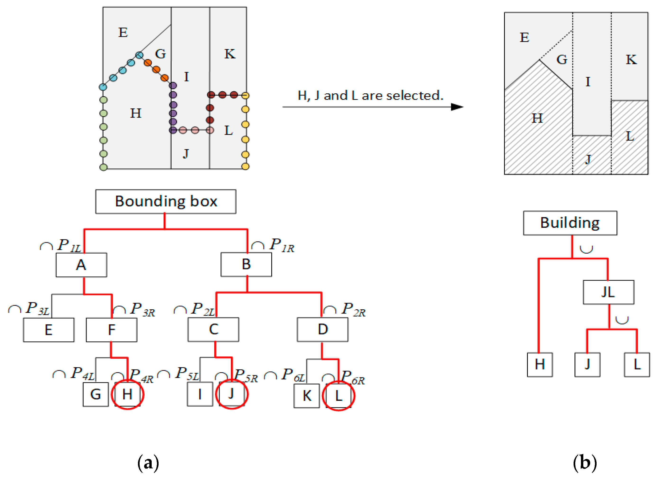
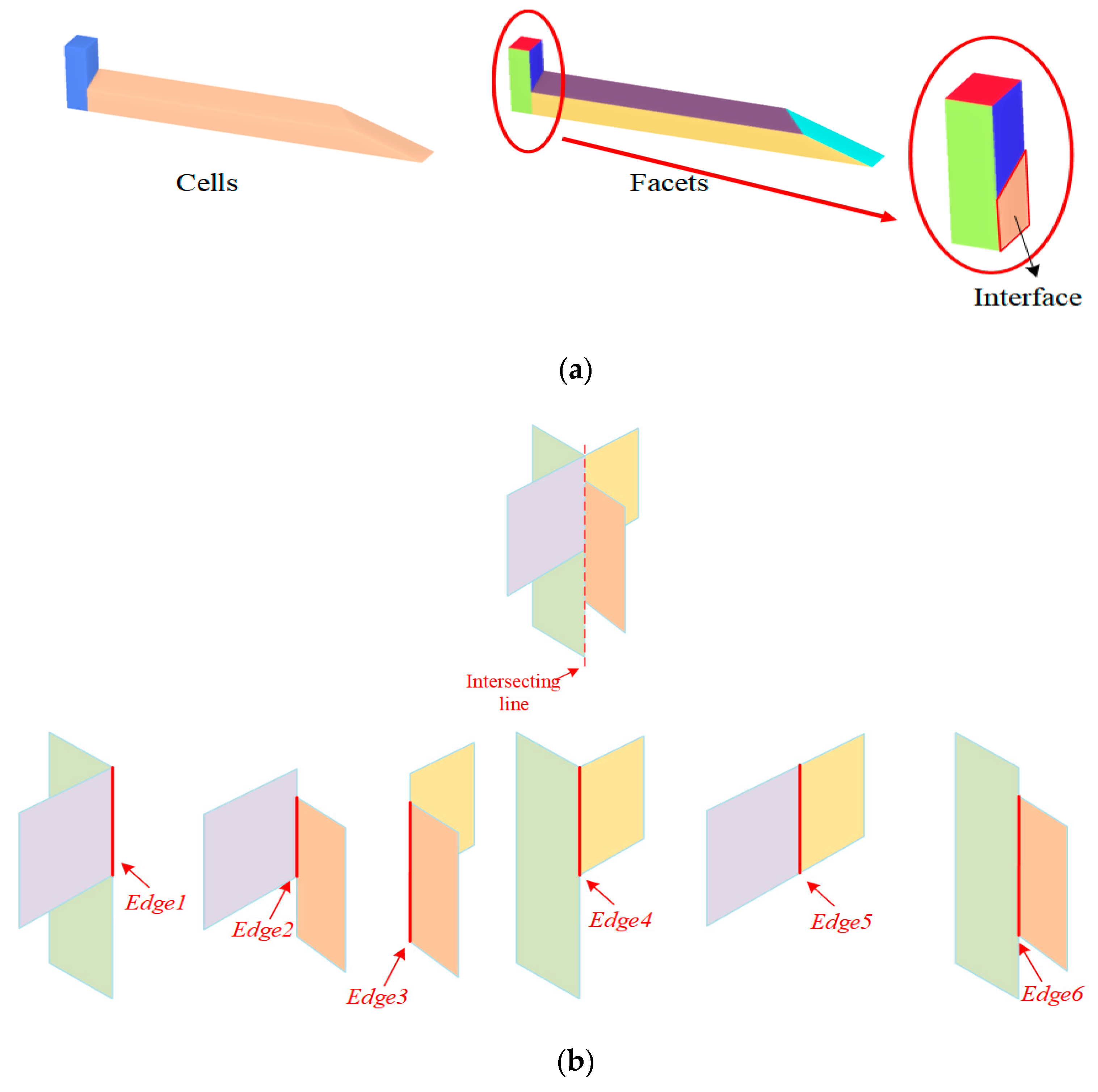
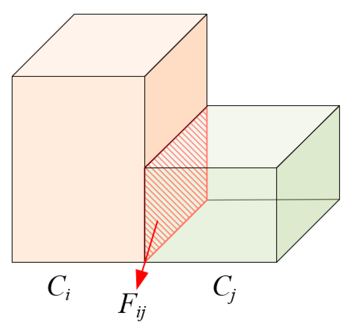
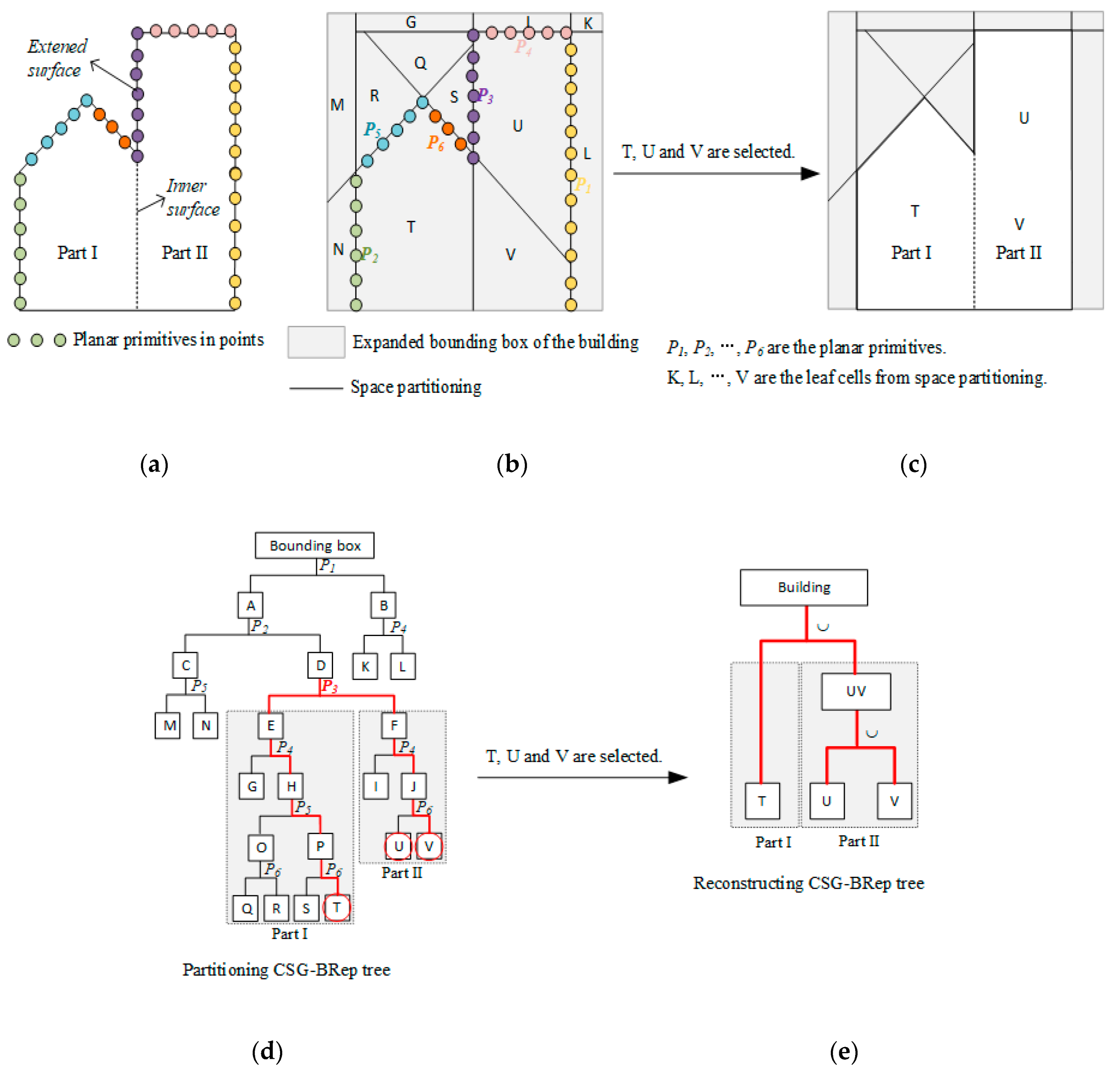
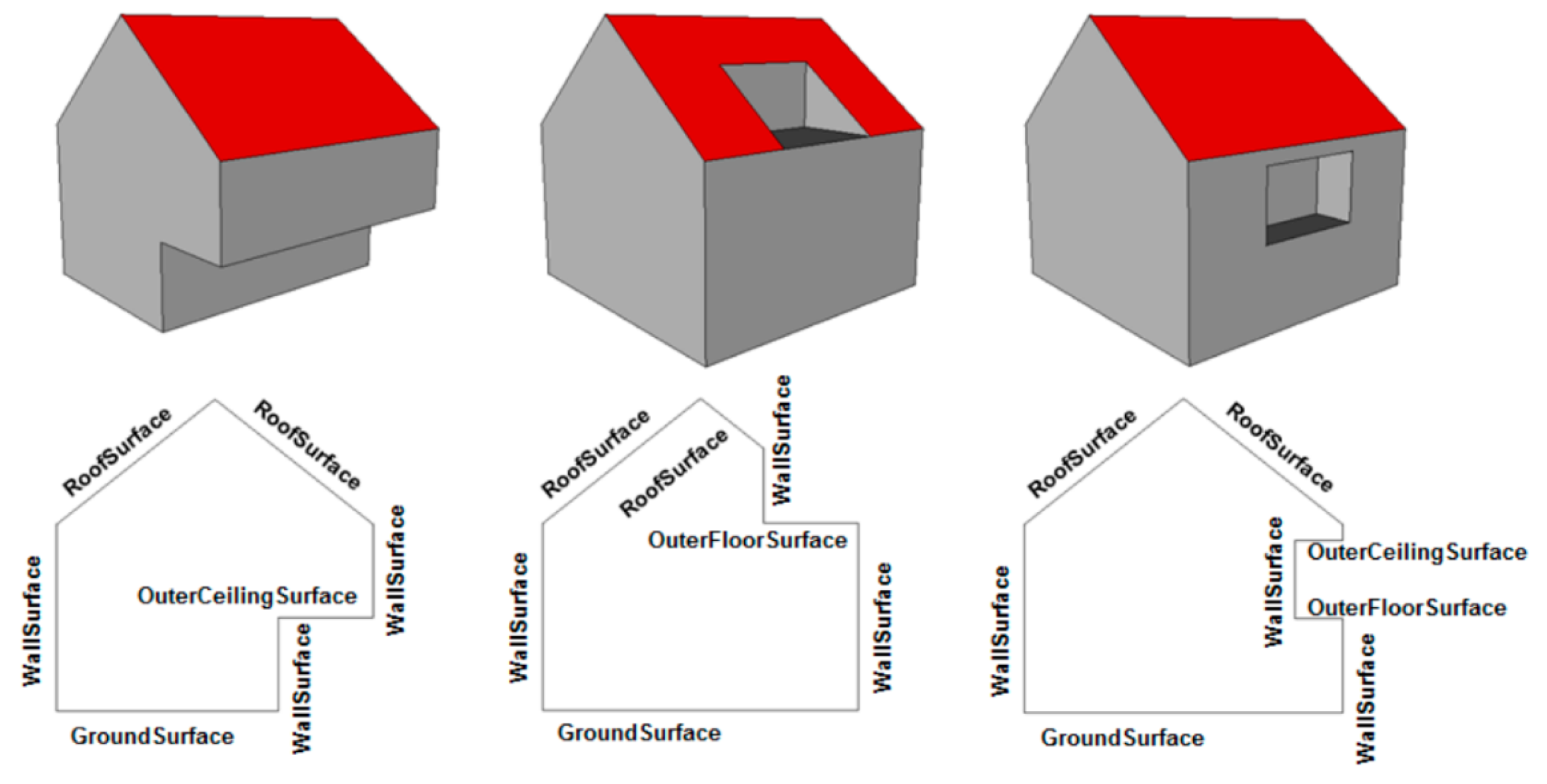
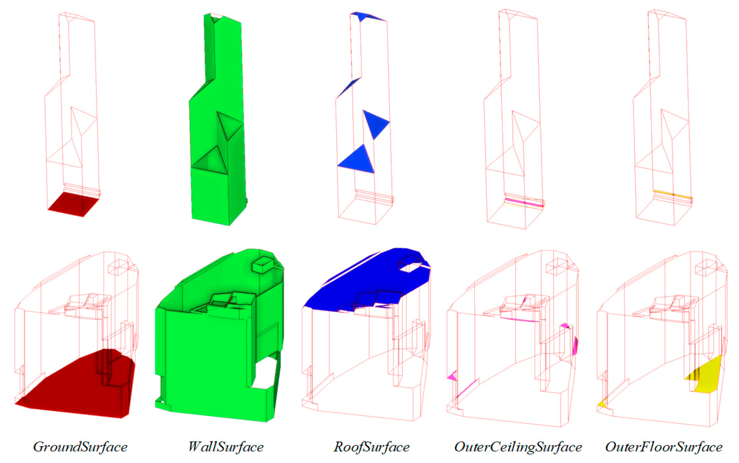
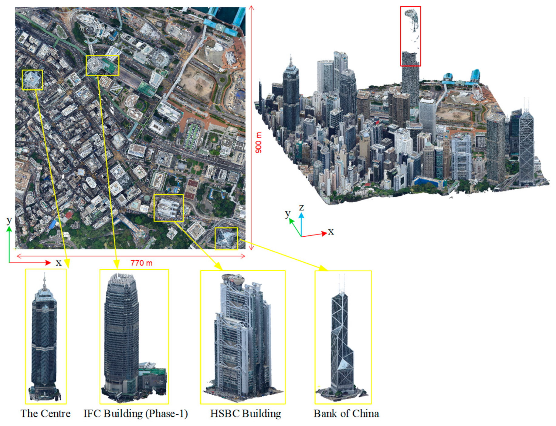
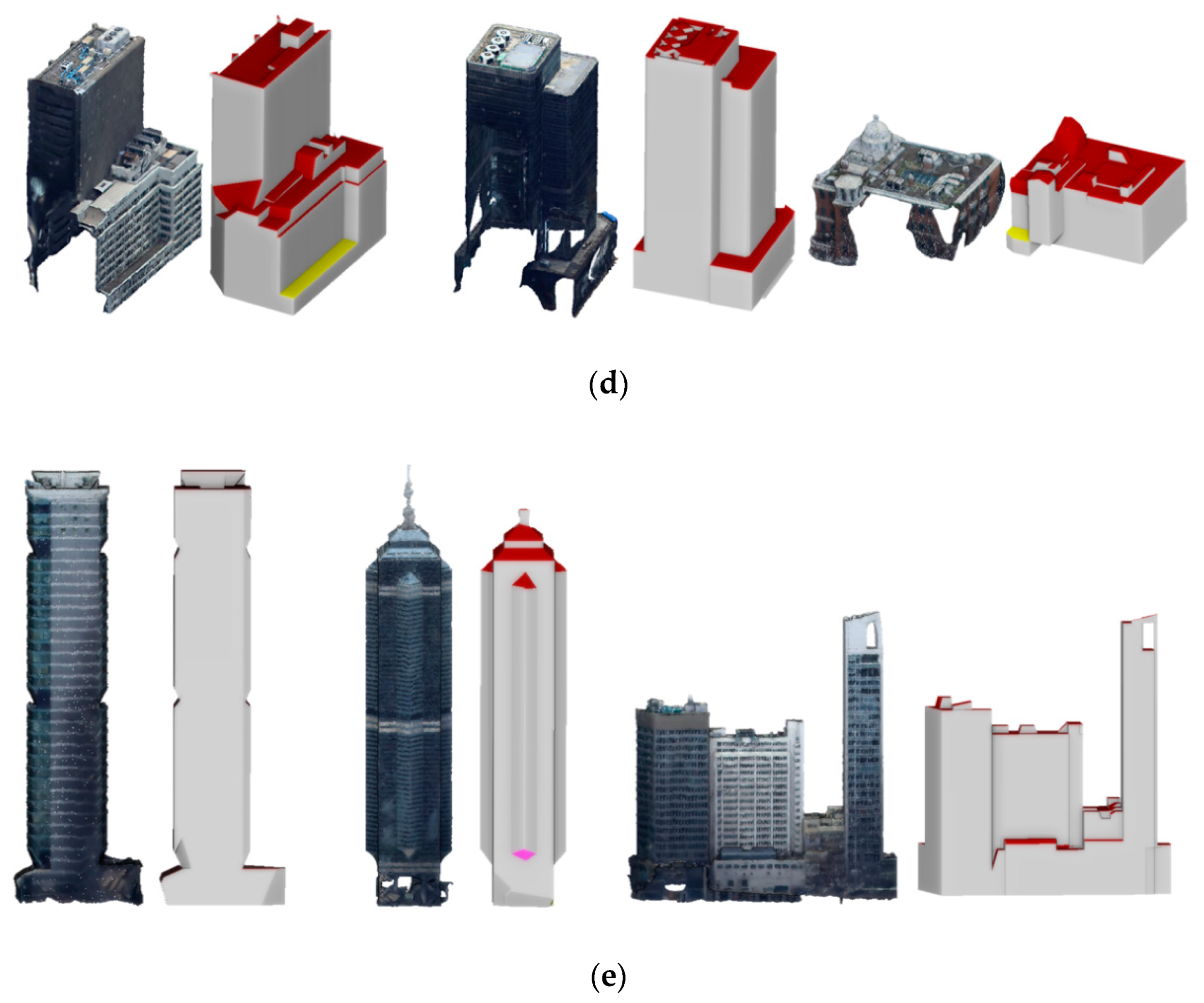
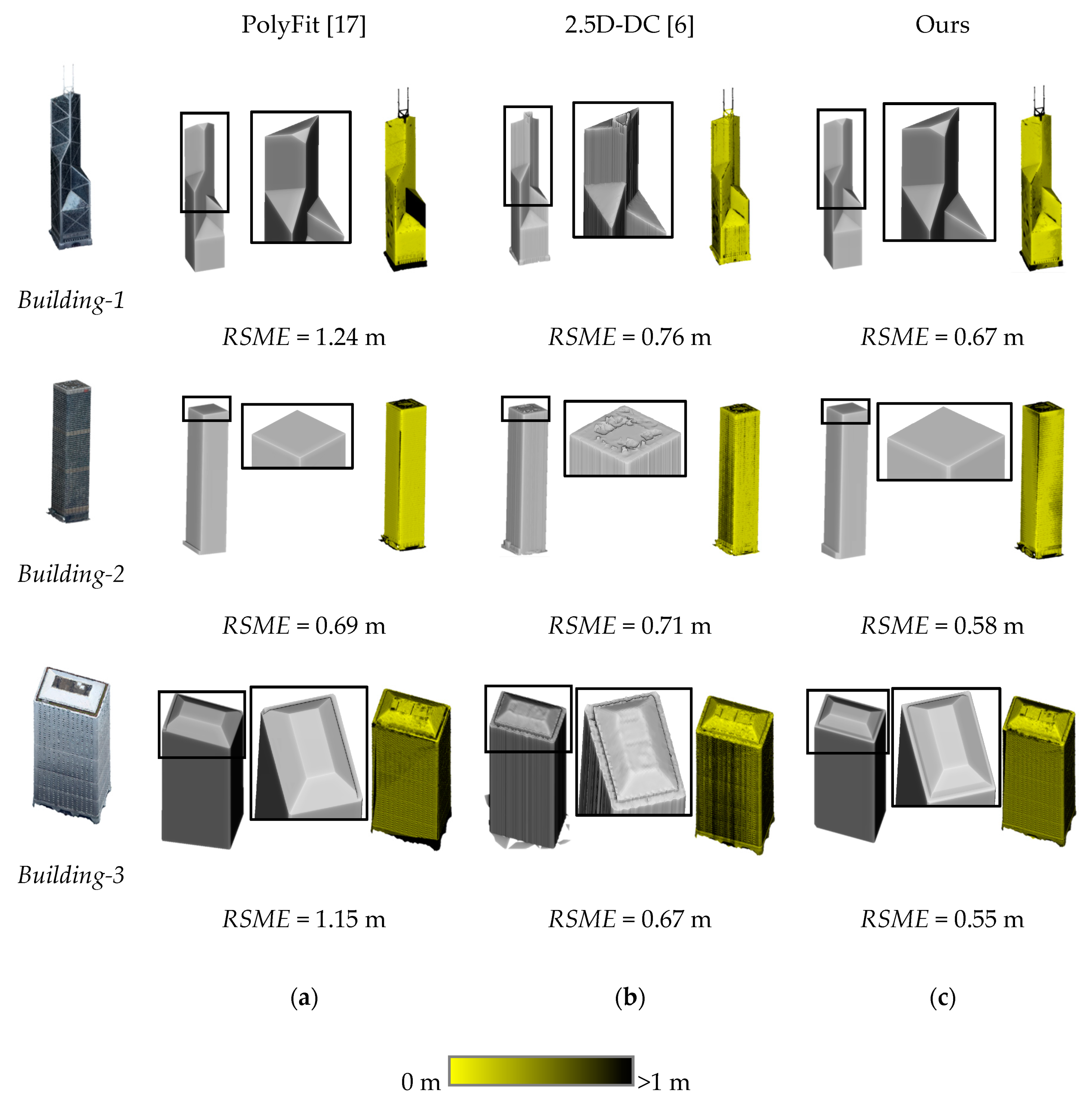
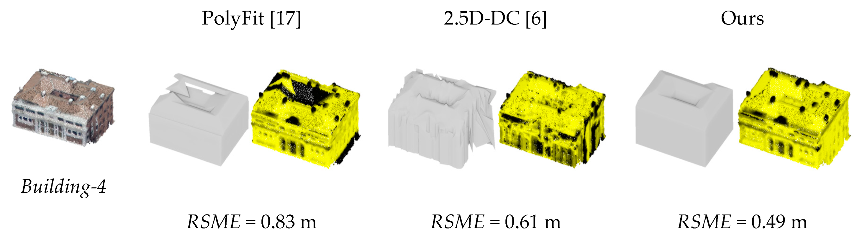
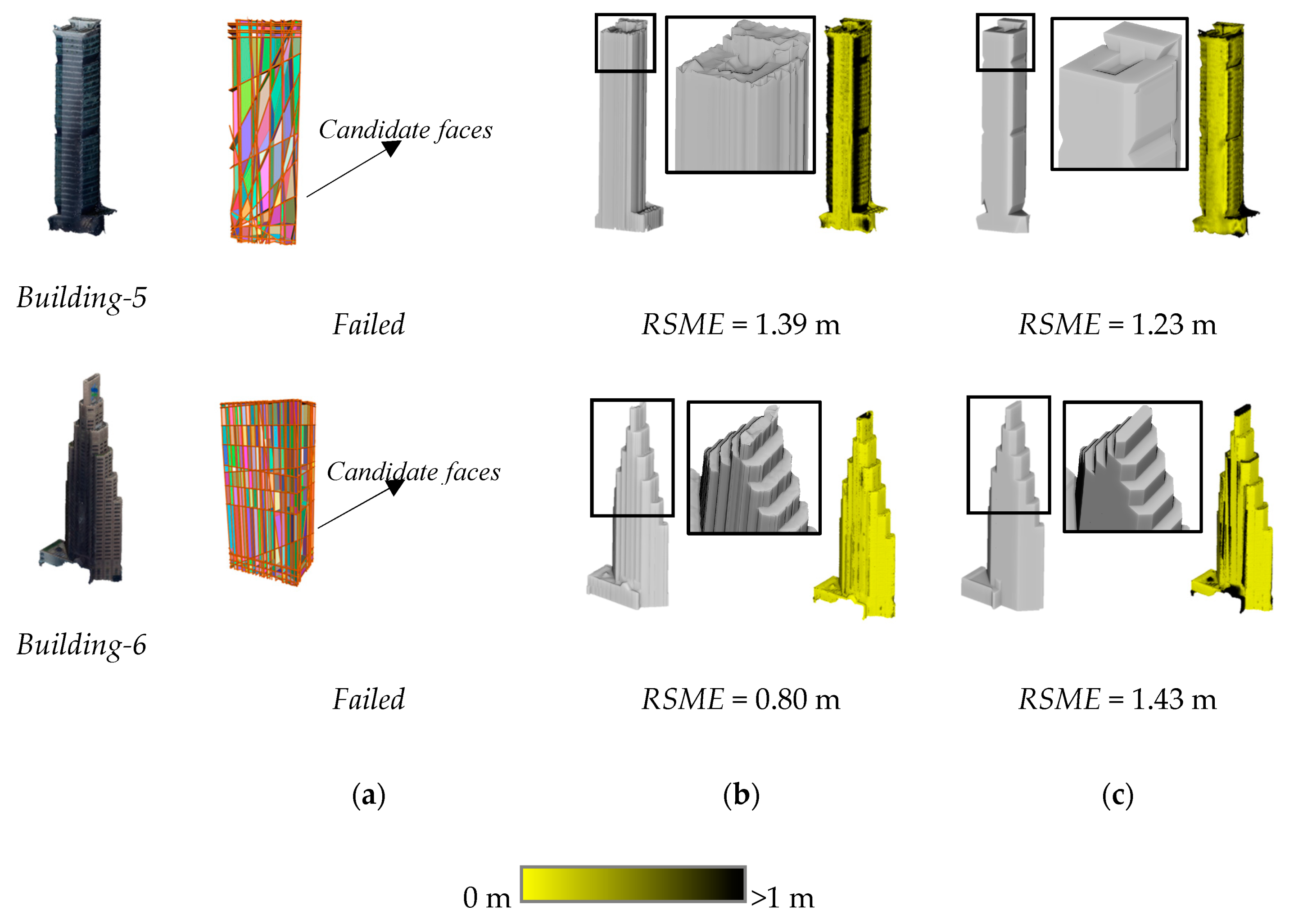
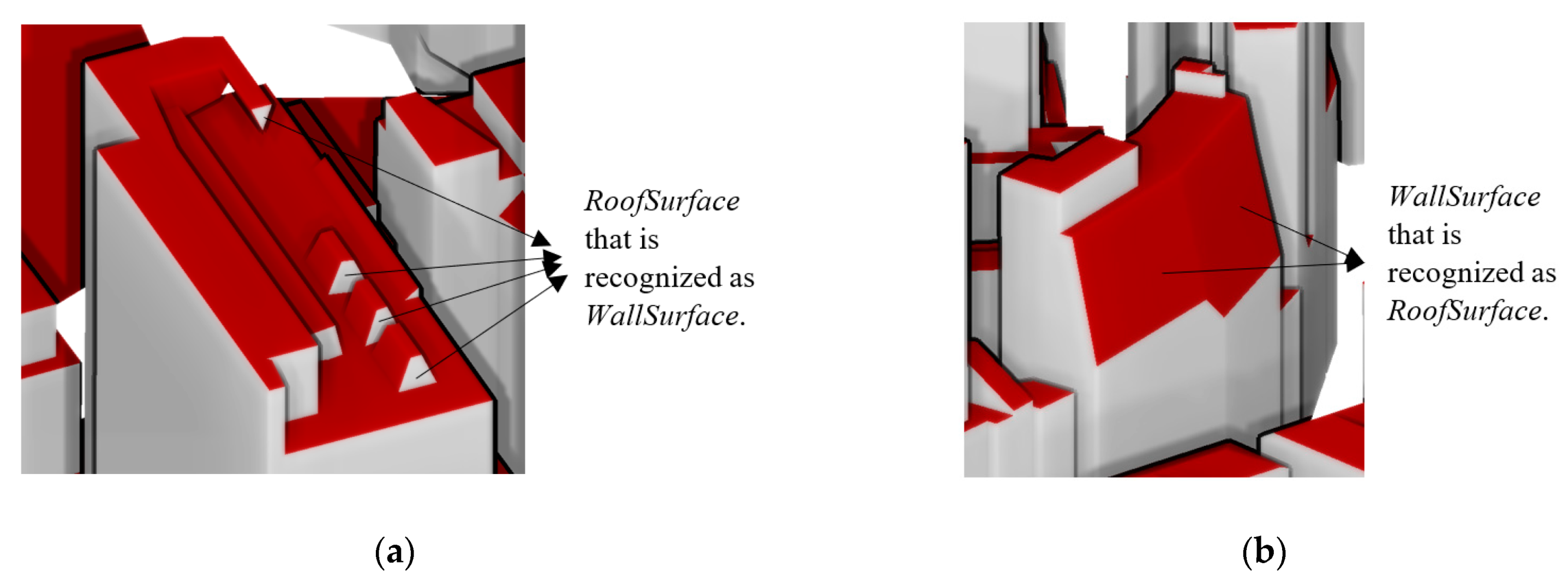
Table 1.
Geometric relations used to refine the planar primitives of buildings.
| Relation Type | Description |
|---|---|
| Horizontality | Pi is vertical if θ (ni, nz) < ε. |
| Verticality | Pi is vertical if θ (ni, nz) > π/2 − ε. |
| Parallelism | Pi and Pj are parallel if θ (ni, nj) < ε. |
| Orthogonality | Pi and Pj are orthogonal if θ (ni, nj) > π/2 − ε. |
| Z-symmetry | Pi and Pj are z-symmetric if |θ (ni, nz) − θ (nj, nz)| <ε. |
| XY-parallelism | Pi and Pj are xy-parallel if θ (i, ) < ε. |
| Co-planarity | Two parallel plane primitives Pi and Pj are co-planar if |di − dj| < d. |
Table 2.
2D topological relations between facet projections and the corresponding operations.
| Topological-Relation | Output | Operations | ||
|---|---|---|---|---|
 | Separated |  | Add Fi to F1. | |
 | Connecting |  | Add Fi to F1. | |
 | Full-overlapping |  | Remove Fj from F1; add Fij to F2. | |
 | Partially-overlapping 1 |  | Remove Fj from F1; add Fij to F2; add Fj’ to F1. | |
 | Partially-overlapping 2 |  | Remove Fj from F1; add Fij to F2; add Fi’ to F1. | |
 | Partially-overlapping 3 |  | Remove Fj from F1; add Fij to F2; add Fj’, Fj’’ to F1. | |
 | Partially-overlapping 4 |  | Remove Fj from F1; add Fij to F2; add Fi’, Fi’’ to F1. | |
 | Contained |  | Remove Fj from F1; add Fij to F2; add Fj’, Fj’’ to F1. | |
 | Containing |  | Remove Fj from F1; add Fij to F2; add Fi’, Fi’’ to F1. | |
 | Intersecting |  | Remove Fj from F1; add Fij to F2; add Fi’ to F1; and Fj’ to F1. | |
Table 3.
1D topological relations between the co-linear 3D edges and corresponding operations.
| Topological-Relation | Output | Operations | |
|---|---|---|---|
 | Separated |  | Add Ei to E1. |
 | Connecting |  | Add Ei to E1. |
 | Fully-overlapping |  | Remove Ej from E1; add Eij to E2. |
 | Partially-overlapping1 |  | Remove Ej from E1; add Eij to E2; add Ej’ to E1. |
 | Partially-overlapping2 |  | Remove Ej from E1; add Eij to E2; add Ei’ to E1. |
 | Contained |  | Remove Ej from E1; add Eij to E2; add Ej’, Ej’’ to E1. |
 | Containing |  | Remove Ej from E1; add Eij to E2; add Ei’, Ei’’ to E1. |
 | Intersecting |  | Remove Ej from E1; add Eij to E2; add Ei’ to E1; add Ej’ to E1. |
Table 4.
Knowledge-based rules for determination of building surface type.
| Normal Direction | Elevation Information | Surface Type | |
|---|---|---|---|
| |θ (n’,nz)| ≥ π/2 − ε | - | WallSurface | |
| ε < |θ (n’, nz)| < π/2 − ε | n’, nz > 0 | - | RoofSurface |
| n’, nz < 0 | - | WallSurface | |
| |θ (n’, nz)| ≤ ε | n’, nz > 0 | < zmin + (zmax − zmin)/3 and < 10 m | OuterFloorSurface |
| otherwise | RoofSurface | ||
| n’, nz < 0 | < zmin + d | GroundSurface | |
| otherwise | OuterCeilingSurface | ||
Table 5.
Quantitative evaluation of building surface classification..
| GT | Ground Surface | Wall Surface | Roof Surface | OuterFloor Surface | OuterCeiling Surface | Precision |
|---|---|---|---|---|---|---|
| GroundSurface | 105 | 0 | 0 | 0 | 0 | 100% |
| WallSurface | 0 | 4170 | 242 | 0 | 0 | 95% |
| RoofSurface | 0 | 104 | 2735 | 0 | 0 | 96% |
| OuterFloorSurface | 0 | 0 | 0 | 24 | 0 | 100% |
| OuterCeilingSurface | 0 | 0 | 0 | 0 | 241 | 100% |
| Recall | 100% | 98% | 92% | 100% | 100% |
Publisher’s Note: MDPI stays neutral with regard to jurisdictional claims in published maps and institutional affiliations. |
© 2021 by the authors. Licensee MDPI, Basel, Switzerland. This article is an open access article distributed under the terms and conditions of the Creative Commons Attribution (CC BY) license (http://creativecommons.org/licenses/by/4.0/).
Share and Cite
MDPI and ACS Style
Li, Y.; Wu, B. Relation-Constrained 3D Reconstruction of Buildings in Metropolitan Areas from Photogrammetric Point Clouds. Remote Sens. 2021, 13, 129. https://0-doi-org.brum.beds.ac.uk/10.3390/rs13010129
AMA Style
Li Y, Wu B. Relation-Constrained 3D Reconstruction of Buildings in Metropolitan Areas from Photogrammetric Point Clouds. Remote Sensing. 2021; 13(1):129. https://0-doi-org.brum.beds.ac.uk/10.3390/rs13010129
Chicago/Turabian StyleLi, Yuan, and Bo Wu. 2021. "Relation-Constrained 3D Reconstruction of Buildings in Metropolitan Areas from Photogrammetric Point Clouds" Remote Sensing 13, no. 1: 129. https://0-doi-org.brum.beds.ac.uk/10.3390/rs13010129
Note that from the first issue of 2016, this journal uses article numbers instead of page numbers. See further details here.