Deriving Tree Size Distributions of Tropical Forests from Lidar


1
Department of Ecological Modelling, Helmholtz Centre for Environmental Research—UFZ, 04318 Leipzig, Germany
2
German Centre for Integrative Biodiversity Research (iDiv), 04103 Halle-Leipzig-Jena, Germany
3
Institute of Environmental Systems Research, University Osnabrück, 49076 Osnabrück, Germany
*
Author to whom correspondence should be addressed.
Remote Sens. 2021, 13(1), 131; https://0-doi-org.brum.beds.ac.uk/10.3390/rs13010131
Submission received: 14 November 2020
/
Revised: 20 December 2020
/
Accepted: 30 December 2020
/
Published: 2 January 2021
Abstract
:Remote sensing is an important tool to monitor forests to rapidly detect changes due to global change and other threats. Here, we present a novel methodology to infer the tree size distribution from light detection and ranging (lidar) measurements. Our approach is based on a theoretical leaf–tree matrix derived from allometric relations of trees. Using the leaf–tree matrix, we compute the tree size distribution that fit to the observed leaf area density profile via lidar. To validate our approach, we analyzed the stem diameter distribution of a tropical forest in Panama and compared lidar-derived data with data from forest inventories at different spatial scales (0.04 ha to 50 ha). Our estimates had a high accuracy at scales above 1 ha (1 ha: root mean square error (RMSE) 67.6 trees ha−1/normalized RMSE 18.8%/R² 0.76; 50 ha: 22.8 trees ha−1/6.2%/0.89). Estimates for smaller scales (1-ha to 0.04-ha) were reliably for forests with low height, dense canopy or low tree height heterogeneity. Estimates for the basal area were accurate at the 1-ha scale (RMSE 4.7 tree ha−1, bias 0.8 m² ha−1) but less accurate at smaller scales. Our methodology, further tested at additional sites, provides a useful approach to determine the tree size distribution of forests by integrating information on tree allometries.
1. Introduction
Forests shape the Earth’s ecosystem, covering more than 30% of land area worldwide and storing about 45% of the terrestrial carbon [1,2,3]. They represent an important habitat for biodiversity and are relevant for economy and society [4,5]. At the same time, they are increasingly affected by climate warming and weather extremes [6,7,8], logging and fire [5], deforestation and fragmentation [5,9,10,11,12].
To conserve forests, their current status and future development must be monitored. In the past, the state of a forest has been determined using field measurements of sample plots (e.g., 1 ha). Recent studies, in turn, gathered large-scale plot data (e.g., 50 ha), regularly collecting detailed information such as the stem diameter or the species and location of each tree [13]. Over recent decades, remote sensing has become an increasingly used tool to monitor the state of forests [14,15].
Remote sensing techniques like light detection and ranging (lidar) (terrestrial, airborne or spaceborne, e.g., Ice, Cloud, and land Elevation Satellite (ICESat) [16], Global Ecosystem Dynamics Investigation (GEDI) [17]), radar (e.g., TerraSAR-X-Add-on for Digital Elevation Measurements (TanDEM-X) [18], Advanced Land Observing Satellite (ALOS), Phased Array type L-band Synthetic Aperture Radar (PALSAR) [19]) and optical reflectance (Landsat [20], Sentinel [21] or Moderate-resolution Imaging Spectroradiometer (MODIS) [22]) provide information on forests at different spatial and temporal resolutions. Earth observations have been used to gain insight on (a) forest cover, (b) forest biomass, and (c) forest structure. For example, global forest cover has been explored from Landsat data at the 30-m resolution [3] and has been used for the analysis of deforestation, forest fragmentation [9], and their respective drivers [10].
Often, remote sensing observations have been analyzed by computing correlations with forest attributes (e.g., lidar metrics correlated with biomass or basal area) [23,24,25,26,27,28]. Such approaches have a high predictive power, but typically focus on predicting single forest attributes (like biomass) and require field-data-intensive calibration of site-specific parameters in the statistical relationships. Studies also combined statistical methods with information on tree geometry [29,30,31]. A good example for an approach that integrates tree geometry is Spriggs et al. [30], who combined allometric relations with a Bayesian optimization approach.
Recent studies have followed the approaches of tree segmentation [32,33,34,35,36] by detecting single tree crowns from airborne lidar to estimate tree size attributes and frequencies. Those techniques interpret lidar point clouds and allow the detection of tree geometry relations (in particular for large trees). Similar approaches also use information from terrestrial lidar [37] with its strength to detect detailed tree leaves and branches, particularly in the lower canopy (often constrained to small forest plots). Both approaches require high-resolution lidar point clouds to have sufficient information on the trees.
Here, we present a novel approach for inferring forest structure from lidar measurements that is complementary to the recent approaches. Our approach integrates the available information on tree geometry in a theoretical model. Through its combination with the measured vertical lidar profile (e.g., derived from waveforms or lidar point clouds), we calculated how many trees of a certain size could occur in a forest to match the measured profile (Figure 1). This allowed us to estimate the tree size distribution of a forest (i.e., number of trees in different stem diameter classes) based on lidar measurements.
We tested our approach on a 50-ha forest plot in Panama. After determining the leaf–tree matrix, we derived the stem diameter distribution from lidar by applying classical methods of mathematics (matrix inversion). We validated the estimated stem diameter distribution by using field inventory data and demonstrated the accuracy of our approach at different spatial scales (50, 25, 5, 1, 0.25, and 0.04 ha). We analyzed how reliably we can estimate tree numbers per stem diameter class. In addition, we derived estimates for the total stem number and basal area from the lidar measurements.
2. Materials and Methods
2.1. Study Site
We applied our approach to a tropical forest located on Barro Colorado Island in Panama (BCI, 9°9′ N, 79°51′ W) [38,39,40,41], where a 50-ha plot of old-growth tropical moist forest has been monitored every five years since 1980. The study site is located in a natural reserve area in the center of the island. In each census, each tree was tagged and mapped, its species was identified and its stem diameter was measured at breast height. In our study, we used the census of the year 2010, considering all trees of stem diameter ≥ 1 cm. The analyzed forest census included 244,269 trees and 301 tree species (1.5% of the originally recorded trees were disregarded because they were dead or lost, see Supplementary S1). The forest inventory data can be requested from the ForestGeo Global Earth Observatory Network [42] or downloaded for free from Dryad [43].
To relate the height and crown dimension of a tree to its stem diameter, we used three allometric equations:
- (a)
- h = (57.4 × d)/(0.43 + d),
- (b)
- andcr = 9.08 × d0.68
- (c)
- vertical tree crown length cl (m) is linearly related to the tree height by [23]cl = 0.4 × h.
The tree crown radius, length and the assumed shape were used to calculate the tree crown volume, which is multiplied with a density factor of ρ = 0.44 m²/m³ to estimate the tree leaf area [23]. The tree height and crown length were used to estimate the leaf area of a tree at different heights within the forest canopy (we assumed that trees’ leaves are homogenously distributed within their crown).
Tree allometries have been derived from independent field studies [23,24,44,45]. Here, we averaged tree allometries across occurring tree species, which has been shown to be a valid approach when studying the forest structure [46]. In the standard case, we assumed that tree crowns have an ellipsoidal shape, but we tested different crown shapes (spheres and cylinders) as well. We further tested the sensitivity of different allometries for tree height (non-asymptotic power law of tree height [45])
and of leaf density within crowns (factor of ρ = 1 m²/m³).
h = 43.4 × d0.6
Airborne lidar data were available for the 50-ha forest plot for the year 2009 [47]. The point densities ranged from 0 to 103 m−2 (in flight swath overlaps) with a median of 19 m−2. The point cloud was terrain-normalized and thinned using random subsampling to obtain a near homogeneous point density of four returns per m². The latter was achieved by iterative subsampling to different point densities and inspection of the resulting density rasters until no further density differences from the flight pattern were visible. The thinned point cloud contained 19% of the returns from the original point cloud. For details on the instrumentation and processing of the lidar data, see Lobo and Dalling [47] (Materials and Methods). The lidar dataset is publicly available and can be requested from J.W. Dalling (see statement on data accessibility in [47]).
2.2. Derivation of Leaf Area Profiles from lidar
The lidar data (i.e., lidar profile) includes information on the site-specific forest structure as lidar signals get reflected by the leaves and branches of trees. We assumed that the point density PD (1/m²) of the lidar profile in a specific height layer (h(i−1),hi) of constant width Δh = 1 m is a result of (a) the tree crown density (LAD) at which lidar signals could get reflected and (b) the probability (W) that the lidar signal could penetrate into the respective height layer i (i.e., has not already been reflected in the layers above):
PDi = l × LADi × Wi
The parameter l represents a density factor (here, l = 1 m²/m³) that combines different aspects: the density of lidar shots sent to the forest canopy, the fraction of tree leaves (relative to tree branches) at which signals can be reflected and the density of successful lidar signals returned at the top of the forest (due to gaps in the canopy).
The observed lidar point density PDi in (m-²) is then defined as
with the plot area A (m²), the total number of lidar points K and
The sum of the function δik yields the number of lidar points with the return height zk (m) in the respective height layer i. To compute the probability W, we used the Beer–Lambert law of light transmission and extinction [48].
where ΣLADj is the cumulative leaf area density (m²/m³) from the top of the forest (j = n) down to the height layer j = i+1. The parameter k in Equation (8) represents the average light extinction coefficient (k = 0.2 for near-infrared or infrared signals with wavelengths of 600–1400 µm) [48].
Based on Equation (5), we can then recursively estimate the forest’s leaf area profile (LADlidar) via
starting with a height layer above the forest canopy (i.e., LADn = 0 results in Wn = 1). We did not include ground returns in our approach and considered only height layers ≥ 3 m. The values of the parameters k and l are relevant for the derived leaf area profile, but had only minor influence on the estimation of the stem diameter distribution in our study (Figure A1).
2.3. ‘Leaf–Tree Matrix’ of the Tree Geometry Model
To estimate the number of trees for different stem diameter classes (here, assumed to be unknown) from the lidar-derived leaf area profile, we developed a theoretical model that integrates the available information on tree geometry and allometry.
For this, we introduced the ‘leaf–tree matrix’. The matrix summarizes the consequences of the assumed tree allometries (see Section 2.1) in a virtual forest in which exactly one tree is present for each stem diameter class. Figure 2 visualizes this matrix, which contains for each stem diameter class (columns) and height layer (colored rows) the corresponding leaf area per tree. White cells indicate that trees in the corresponding stem diameter class do not have leaves in the respective height layer. Height layers are defined in 1-m width, and stem diameter classes (of increasing width) correspond to the respective height layers (based on the assumed stem diameter-height relation, Section 2.1). Each tree has a maximum height (upper boundary of the height layer, based on the tree height allometry and diagonal entries of the matrix). Crowns reach only into the lower height layers (according to the tree crown allometry). Leaf area was assumed to be proportional to the tree crown volume (based on the tree crown allometry) and distributed uniformly among the crown-covered height layers (Section 2.1). See Figure A2 for the leaf–tree matrix with different assumed crown shapes and model assumptions.
As a consequence, the vertical leaf area distribution for a forest with only one tree per stem diameter class can be derived by summing up all column entries (i.e., stem diameter classes) per row (i.e., height layers) in the leaf–tree matrix.
We denote the leaf–tree matrix by F = (fij) with i,j = 1, …, n and the number of trees for each stem diameter class i by the vector N = (Ni)i=1,...,n (with n being the number of stem diameter classes, here n = 55). Multiplying the leaf–tree matrix F with the vector N results in the leaf area profile of a forest plot (LAD in m²/m³), in which we normalize by the plot area A (m²) and height layer width Δh (m)
We aim to develop an approach to infer the stem diameter distribution based on lidar measurements. Therefore, we assumed that sufficient information about forest structure was included in the lidar-derived leaf area profile (LADlidar of Equation (9)), which was used for the LAD (of Equation (10)). Rearranging Equation (10) yields the stem diameter distribution (unknown vector N).
2.4. Linear Equation Solving to Derive Forest Structure from lidar Profiles
Equation (10) represents a system of n linear equations with n unknowns. To rearrange this equation for inferring the unknown stem diameter distribution (vector N), the inverse of the leaf–tree matrix F is required. Since, by construction, the height of trees in the n-th stem diameter class never exceeds the n-th height layer, all above-diagonal matrix entries are zero. This makes the leaf–tree matrix F a lower triangular matrix, which is invertible (n × n matrix) [49]. Rearranging Equation (10) for the vector N then results in
Though Equation (11) yields the number of trees (N) for each stem diameter class, some of the computed values can be negative. Therefore, we developed an iterative numerical backward approach for solving the linear equation system of Equation (10) (using LADlidar to represent LAD). See Appendix A Table A1 for a comparison of results between the direct and numerical calculation and Appendix B for details on the algorithm of numerical calculation.
2.5. Analysis and Statistics of Results
We evaluated the accuracy of our approach by comparing the estimated stem diameter distribution with forest inventory data (i.e., stem numbers per ha and stem diameter class). To compare the stem diameter distribution observed in the field with that estimated from lidar data and our tree geometry model , we performed a logarithmic regression analysis, setting with the intercept I and the regression slope s. We analyzed the regression slope s and the coefficient of determination R² for stem diameter classes with stem numbers larger than zero only (in both inventory and estimates). Optimal values of R² = 1 and s = 1 would reflect the highest achievable accuracy of the lidar -derived tree numbers.
We further calculated the root mean square error RMSE (in trees per ha)
and its normalized counterpart nRMSE (in %, using the range of censused stem numbers across all stem diameter classes to normalize)
with being the plot area in ha. We calculated both RMSE and nRMSE for (non-logarithmic) stem numbers aggregated to 10 cm stem diameter classes and for trees with stem diameter d ≥ 10 cm.
We further estimated the total tree density (N) and basal area (BA) of the forest based on the lidar-derived stem diameter distribution (using stem diameter classes of the leaf–tree matrix and class mid values for basal area estimates) and compared them with the field inventory. Again, we focused on classes with stem diameter above 10 cm. In addition, we compared the tree density and basal area estimates also for each 10-cm aggregated stem diameter class (j) with the inventory
To assess the accuracy of our approach on different spatial scales, we varied the size of the analyzed plot. First, we applied our approach at the scale of 50 ha (entire forest plot). In a second step, we divided the forest plot into subplots of equal sizes of, respectively, 25, 5, 1, 0.25, and 0.04 ha. Subplot sizes of 25 × 25 m or lower are especially interesting as they correspond to the size of the footprint of satellite-based lidar observations (GEDI [17]). For a specific plot size, we calculated, for each subplot, the nine statistical measures (regression slope, R², RMSE, nRMSE, tree density, and basal area in total and absolute differences per 10-cm stem diameter class). For each spatial scale, we calculated the arithmetic mean, standard deviation, and range of the statistical measures across the respective subplots. For the mean values of R², regression slope, RMSE, and nRMSE, we used linear regression to identify scaling relations expressing these statistical quantities as functions of the plot size. To compare the estimated tree density and basal area with inventory data, we used linear regression, computed the bias (average difference of field from lidar-derived attribute), RMSE and nRMSE (normalized by the mean of the observed attribute).
We further correlated the R² values we obtained for the estimated stem diameter distribution (per subplot) (a) with the other obtained statistical measures (RMSE, nRMSE, and regression slope for the stem diameter distribution), (b) with characteristics of the lidar-derived leaf area profile (e.g., median profile height), and (c) forest attributes (e.g., tree density and basal area). For a full list of attributes used for the correlations, see Table 1. We evaluated each correlation by calculating Spearman’s rank correlation coefficient r.
3. Results
3.1. Stem Diameter Distribution Derived at the 50-ha Scale
The stem diameter distribution of the 50-ha forest plot shows a typical heavy-tailed pattern, as often observed in old-growth forests, with few large trees and numerous small ones (Figure 3a, linear appearance on log–log axes). To test our approach at the 50-ha scale, we derived the stem diameter distribution from lidar and compared the estimated tree numbers per stem diameter class with the observed numbers from the inventory (Figure 3). The stem diameter distribution was estimated from lidar with a high accuracy (RMSE = 22.8 tree per ha, nRMSE = 6.2%, R² = 0.89, Figure 3, Table A1).
The number of mid-sized and large trees was estimated accurately (10 cm < stem diameter ≤ 50 cm with RMSE = 39.4 trees per ha, stem diameter > 50 cm with RMSE = 1.2 trees per ha) while trees smaller than 10 cm in stem diameter were overestimated (RMSE = 590.5 trees per ha, Figure A3a). Based on the lidar-derived stem diameter distribution, the estimated tree density of 516.7 trees per ha (stem diameter d ≥ 10 cm) slightly overestimated the censused density of 447.3 trees per ha (bias of −69.4 trees per ha). The basal area estimates showed in turn, a slight underestimation (inventory: 30.1 m²/ha, lidar: 23.6 m²/ha, bias: 6.5 m²/ha, Figure A3a). A sensitivity analysis revealed only minor influences of differently assumed crown shapes, tree height allometry or the leaf density within crowns (Table 2, Figure A2).
3.2. Small-Scale Derivations of Stem Diameter Distributions
We tested our approach also for smaller plot sizes (25, 5, 1, 0.25, and 0.04 ha, Table 3, Table A2). For most plot sizes (e.g., at the 1-ha and 0.25-ha scale), the stem diameter distributions were estimated well from the lidar data (Figure 4a–f, e.g., average R² values of 0.76 and 0.67, average RMSE values of 67.6 and 118.1 trees per ha, Figure A4). Few plots at the 0.25-ha scale showed lower R² (down to 0.13), higher RMSE values (up to 385.6 trees per ha) or higher nRMSE values (up to 105.7%) (Figure A4). At the 0.04-ha scale, more plots with lower accuracy of the estimated stem diameter distribution occurred; nevertheless, we obtained a mean R² of 0.44 (mean RMSE of 219.2 trees per ha, mean nRMSE of 70.9%) (Figure 4i, Table 3, Table A2). Similar results can also be observed for the regression slope (Figure A4). Interestingly, the R² values scaled with plot size (Figure 5, similarly also RMSE, nRMSE, and regression slope) and correlated non-linearly with the other statistical quantities (Table A3; however, the correlations of R² with RMSE or nRMSE were less strong, r = 0.09 and 0.05 at 1-ha scale).
Estimates on the tree density and basal area showed good results for the 1-ha scale with nRMSEs of 51.1% and 15.7%, respectively (bias of −168.2 trees/ha and 0.8 m²/ha, Figure 6, Table 3). The estimation capability for the tree density and basal area per stem diameter class did not change with decreasing plot size (mostly for small-sized classes) but showed larger variations for smaller plots (Figure A3c,d). Interestingly, the forest basal area was best estimated at the 1-ha scale (Figure 6, Figure A5, Table 3, underestimated for larger plot sizes, Table A2), while the tree density was best estimated at the 50-ha scale (Figure 6, Table 3). Both attributes were overestimated by lidar at smaller spatial scales (Table 3, Table A2).
To understand how well stem numbers can be derived from lidar using our approach (e.g., in case no inventories are available), we correlated the R² values of comparing inventory- and lidar-derived stem diameter distributions with other measures characterizing each plot for the spatial scales of 1, 0.25, and 0.04 ha. Those measures describe either the lidar profile or the forest structure (Table 1). We found correlations for the median height of lidar returns WMPH (weighted median profile height, weighted by the derived leaf area density LADlidar, r = −0.19 to −0.31, Table A3) and total tree density (stem diameter d ≥ 1 cm, r = 0.12 to 0.27, Table A3, Figure 7).
The WMPH became more important with increasing spatial scale (as well as variance of leaf area density), while the total tree density showed less strong correlation at larger scales. Interestingly, the tree density, only for stem diameter d ≥ 10 cm, revealed an opposite trend with stronger correlation at the 1-ha scale than at smaller scales (Table A3). This suggests that forest plots characterized by a low and dense canopy could enable a more reliable estimation of the stem diameter distribution from lidar data. In addition, the forest heterogeneity (standard deviation of tree height) also plays a relevant role (r = −0.16 to −0.28, Figure 7c, Table A3). Surprisingly, a reliable estimation of the stem diameter distributions (in terms of high R² values) showed weak correlations with the number of lidar returns, median tree height, and forest basal area (Table A3).
4. Discussion
We presented here a novel approach for estimating the tree size distributions from lidar measurements. Our approach is solely based on the vertical profile of lidar data and infers the number of trees per stem diameter class by integrating the available tree size allometries. On the example of a tropical forest in Panama, we demonstrated that the presented method was able to estimate the stem diameter distribution with high accuracy not only at the 50-ha scale (RMSE of 22.8 trees per ha, nRMSE of 6.2%, R² of 0.89), but also at the 1-ha scale (average RMSE of 67.6 trees per ha, mean R² of 0.76). The basal area was estimated well at the 1-ha scale (bias 0.8 m² ha−1), but the bias increased at smaller scales (−8.0 m² ha−1 at 0.25-ha scale). We identified the most decisive factors for a good estimation of stem diameter distributions at smaller spatial scales as (a) the mean profile height (WMPH), (b) tree density, and (c) forest heterogeneity (in terms of tree height).
The change from a still good estimation of stem diameter distributions at larger spatial scales (50 ha to 0.25 ha) toward slightly biased estimates at the 0.04-ha scale probably could be related to the crown overlapping of large trees and edge effects (crowns from trees of neighboring plots). This might also affect the identified correlations between the goodness of fit and forest attributes, which are not strong (maximum values of 0.3 or −0.3, respectively). Forest inventory data including explicit tree locations allowed us to calculate the overlapping crown parts from neighboring plots and, thus, enabled us to quantify and to account for such effects. Furthermore, we demonstrated our approach on the example of an old-growth tropical forest site (at BCI, Panama). The results of small-scale estimations and the identified correlations could differ for forests of other biomes (like temperate or boreal forests) or for disturbed or managed sites (e.g., logged forests or forest plantations).
4.1. Strengths and Limitations of the Presented Approach
Our approach complements recent methods [23,24,25,26,27,28,29,30,31,32,33,34,35,36] as it (i) integrates already available information on tree geometry (captured in the leaf–tree matrix) and (ii) estimates the full range of size classes in tree size distributions. Tree size distributions can be used to derive different forest attributes (e.g., tree density or forest basal area) and allow us to estimate a forest’s successional state or disturbances [50]. By this, our approach extends statistical methods that often focus on single forest attributes. In comparison to approaches that also integrate tree geometry with statistics, our approach obtained, for almost 85% of the analyzed plots at the 0.25-ha scale, an R² > 0.5 (e.g., Spriggs et al. [30] reached 73% of 0.25-ha plots with an R² > 0.5 in temperate forests). The presented approach complements tree segmentation methods. Such methods show their strength in predicting the size and geometry of large trees, while our approach effectively predicts small- and mid-sized trees in the forest, also at larger spatial scales.
Our approach is based on information about tree allometries, which are available for a wide range of different forest types and biomes (e.g., [44,51], information can also be found in national forest inventories). Tree allometries are assumed a priori in our approach and can differ across regions and forest types. This approach may not be suitable especially for large trees, leaning trees or trees with a complex geometry. We identified only minor influences of these model assumptions on the estimated stem diameter distribution for our study site (Figure A2, Table 2). We demonstrated a good estimation of the forest basal area and total tree density based on lidar-derived tree numbers for stem diameters larger than 10 cm.
To improve the allometries, crown size relations can also be derived by tree crown detection algorithms based on lidar point clouds [32,33,52]. For example, Ferraz et al. [33] reported tree and crown allometries based on detected single trees and their respective uncertainties. This approach requires high-resolution lidar point clouds, particularly for correctly detecting small- and mid-sized trees (with small crowns) in the understory where the lidar point density is normally lower. While our approach shows its strength in estimating tree numbers of small- and mid-sized trees (based on the vertical lidar profile), tree crown detection approaches are especially interesting for applications at smaller spatial scales. Methods based on crown delineation and classification approaches or using terrestrial lidar measurements will, in the future, provide further knowledge on the crown shape of single trees (e.g., National Ecological Observatory Network (NEON)) [53,54].
Our approach includes only average tree size allometries across occurring tree species. We already demonstrated, in a previous study [46], that forest size structure can be explained by using average tree allometry. However, forest sites where crown shapes, in particular, (and the amount of leaf area per crown volume) differ more between tree species will be more difficult to analyze and will require a closer look. In this case, our method could be extended toward a linear combination of multiple leaf–tree matrices (one for each dominant tree species) if information on the species composition is available (e.g., by optical sensors) [55,56]. A recent study [31] demonstrated how stem diameter distributions of different plant functional types can be derived based on site-specific calibration.
Our method is based on vertical lidar profiles only (instead of the full lidar point cloud) and, thus, appears promising for applications to other large footprint lidar data. Previous studies demonstrated the comparability of profiles derived from lidar point clouds and airborne large-footprint waveforms (Land, Vegetation, and Ice Sensor (LVIS)) [57,58]. Two parameters of our methodology (the extinction parameter k and density factor l) for deriving the vertical leaf profile from lidar profiles, could depend on the used remote sensing technique.
While the extinction coefficient k reflects the light extinction in the forest canopy, which depends on the wavelength (e.g., optical vs. near infrared) [48], the density factor l is more phenomenological and might correlate with the used tree allometries. Terrestrial lidar could contribute to the estimation of l for forest plots by reconstructing the detailed tree crown architecture of branches and leaves. We identified only minor influences of both parameters (k and l) on the estimated stem diameter distribution for our study site (Figure A1).
Other methods to derive leaf density profiles from lidar data include similar parameters in their approaches [59,60,61,62]. For example, the method used by Stark et al. [60] and Harding et al. [61] is based on the (logarithmic) ratio of point densities of two adjacent height layers [63] and includes an extinction coefficient. Tang et al. [59] combined the MacArthur–Horn-method with a gap probability approach [64]. The approach of Detto et al. [62], in contrast, is based on a stochastic radiative transfer model and accounts for multiple lidar returns. Methods, like small-footprint full-waveform lidar analyses, could improve estimates on leaf density profiles in the future [65].
4.2. Future Applications and Challenges
Airborne campaigns of lidar measurements have the advantage of providing forest measurements for hundreds of hectares, but are limited to the regional scale and are not able to cover continents. Satellite missions can provide full-waveform lidar data but only provide samples of space (e.g., GEDI has a footprint of 25 m diameter and spacings of 60 m along track and 600 m across track) [17]. Assuming that such spaceborne-generated profiles are comparable with profiles derived from point clouds or airborne-generated waveforms [57], the presented approach could be tested for different remote sensing data and for forest sites at which inventory and spaceborne lidar data is available.
This could be particularly interesting for exploring the site-dependency of tree allometries (and the parameters k and l) in our approach and testing its applicability for a wide range of forest types (especially regions characterized by a heterogeneous forest structure). As our results showed lower quality at smaller spatial scales (of e.g., 0.04 ha), questions on sampling efforts also arise. Do the results improve if we use several plots distant to each other (equivalent to spaceborne lidar footprints)? More specifically, it would be interesting to explore if we can aggregate discontinuously sampled lidar shots over an area to estimate the stem diameter distribution. How many lidar shots are required to be sampled to obtain good estimates of a specific forest site?
Recent studies (based on individual-based forest growth models) [31,66,67] demonstrated how remote sensing information can be combined with forest models to provide additional information about forests. Forest models simulate the long-term dynamics of forests (based on single trees) and can estimate forest successional states by matching simulated and remotely sensed vertical leaf profiles [66]. Our approach—which is based on related methodological assumptions—thus, also appears promising for estimating the successional state (caused, e.g., by disturbances).
As we demonstrated that stem diameter distributions in forest plots with a low dense canopy and low tree height differences can be estimated reliably, we expect that disturbances that occurred previously could be well identified. Challenges for spaceborne lidar could make such an analysis difficult as cloud cover can limit observations and repeated shots will not be located at the same position as before. The latter, however, would be interesting for the tracking of previously logged or disturbed forests. The combination of lidar measurements with other remote sensing techniques (e.g., radar data from the TanDEM-X satellite), thereby, seems promising to allow for an interpolation between lidar shots for large-scale analyses [68].
lidar measurements covering continents and combined with maps of forest cover (e.g., [3]) could enable the calculation of the forest structure and stem diameter distributions at large scale by using the suggested approach if the tree crown allometry is known. Various forest attributes can then also be derived from the estimated lidar-based stem diameter distributions (e.g., forest height, biomass, or basal area) and compared not only with local inventories but also with already existing information, for example, for the Amazon in terms of the basal area or forest biomass [69]. The approach proposed here can, thereby, contribute to the in-depth mapping and monitoring of forests and for supporting sustainable management, conservation, and the protection of forests.
5. Conclusions
We presented a novel approach for predicting the stem diameter distribution of forests based on lidar measurements. Our approach is profile-based and structure-based. This method requires only a vertical lidar profile (instead of point clouds) and integrates the available tree size allometries to infer the number of trees from the profile. By this, our approach complements previous methods based on statistical correlations between lidar and forest attributes or individual tree crown detection methods based on high-resolution lidar point clouds.
We demonstrated, in this study, a test of our approach with good accuracy for an old-growth tropical forest. Further tests of our method for other forest sites (at which tree allometries, lidar data and, for comparison, inventories are available) could help to comprehensively understand the impact of forest stand characteristics and plot size on the accuracy of the estimated stem diameter distributions from lidar.
Supplementary Materials
The following are available online at https://0-www-mdpi-com.brum.beds.ac.uk/2072-4292/13/1/131/s1, Supplementary S1: R-code to calculate the stem diameter distribution of a forest from lidar data.
Author Contributions
Conceptualization, A.H., R.F., and F.T.; Methodology, A.H., F.T., N.K., and R.F.; Software, F.T.; Formal analysis, F.T.; Writing—original draft preparation, F.T.; Writing—review and editing, F.T., A.H., R.F., and N.K.; Visualization, F.T.; All authors have read and agreed to the published version of the manuscript.
Funding
This research received no external funding.
Institutional Review Board Statement
Not applicable.
Data Availability Statement
A publicly available forest inventory dataset was analyzed in this study. This data can be found here (Dryad): https://datadryad.org/stash/dataset/doi:10.15146/5xcp-0d46. The lidar data is publicly available and can be requested from J.W. Dalling. See data accessibility statement and contact details at https://royalsocietypublishing.org/doi/full/10.1098/rspb.2013.3218.
Acknowledgments
The BCI forest dynamics research project was made possible by National Science Foundation grants to Stephen P. Hubbell: DEB-0640386, DEB-0425651, DEB-0346488, DEB-0129874, DEB-00753102, DEB-9909347, DEB-9615226, DEB-9615226, DEB-9405933, DEB-9221033, DEB-9100058, DEB-8906869, DEB-8605042, DEB-8206992, DEB-7922197, support from the Forest Global Earth Observatory, the Smithsonian Tropical Research Institute, the John D. and Catherine T. MacArthur Foundation, the Mellon Foundation, the Small World Institute Fund, and numerous private individuals, and through the hard work of over 100 people from 10 countries over the past three decades. The plot project is part the Forest Global Earth Observatory (ForestGEO), a global network of large-scale demographic tree plots. We further thank J.W. Dalling for providing the lidar data from BCI.
Conflicts of Interest
The authors declare no conflict of interest.
Appendix A
Figure A1.
Sensitivity of the parameters k and l on the accuracy of estimating the stem diameter distribution (50-ha scale). (a) The R² values, (b) the nRMSE (%) values, (c) the difference of the field-derived basal area (30.1 m²/ha) to lidar-derived estimates, and (d) the difference of field-observed tree density (447.3 trees per ha) to lidar-derived estimates are shown for different combinations of parameter values (default values are k = 0.2 and l = 1). The quality of the values is indicated by gradients from green (good quality) to blue and red (lower quality). White cells demonstrate that no solution was possible due to infinite values in the leaf area profile derived from lidar (using the respective parameter combination). (e) The estimated and observed stem diameter distributions compared for selected parameter combinations of k and l.

Figure A2.
Visualization of the leaf–tree matrix and the resulting comparison of the measured tree numbers per stem diameter class (from inventory) with the estimated tree numbers (from lidar) for different sensitivity analysis. Upper graphics: each column in the matrix reflects the leaf area contribution of one tree to different height layers. Different columns represent different stem diameter classes. The leaf area values are shown using a color gradient from light green (low leaf area) to dark green (high leaf area) (white represents no leaf area). Lower graphics: green points show the estimated tree numbers from lidar for each stem diameter class and the grey line shows the observed stem numbers in the inventory. Values of R² and RMSE are given (see Table 3 for further results and a description of changed model assumptions in each scenario).


Table A1.
Results of different calculations (direct: calculation of stem numbers N from Equation 11, numerical backward: numerical solving of Equation 10 for stem numbers N, see methods and Appendix B) to estimate the stem diameter distribution from lidar measurements (50-ha scale)
Table A1.
Results of different calculations (direct: calculation of stem numbers N from Equation 11, numerical backward: numerical solving of Equation 10 for stem numbers N, see methods and Appendix B) to estimate the stem diameter distribution from lidar measurements (50-ha scale)
| Method | Direct Calculation | Numerical Backward Solving |
|---|---|---|
| Regression slope | 1.22 | 1.24 |
| Coefficient of determination R² | 0.88 | 0.89 |
| Number of stem classes with negative predictions (%) | 26.9 | 0 |
| RMSE (trees/ha) | 29.6 | 22.8 |
| nRMSE (%) | 8.1 | 6.2 |
Figure A3.
Evaluation of uncertainties in the lidar-derived tree density (in trees per ha) and lidar-derived basal area (in m²/ha) for three spatial scales: (a) 50 ha, (b) 1 ha, and (c) 0.04 ha. Uncertainties are calculated as the absolute difference of stem numbers or basal area (logarithmic y-axes) per stem diameter class (x-axes) between the results from lidar and field data (points show the mean and the solid line shows the range from minimum to maximum). Note that zero differences are not displayed.

Figure A4.
Spatial maps and histograms of the statistics on RMSE (trees/ha), nRMSE (%), and regression slope for the estimation of stem diameter distributions from lidar, (a–c) at the 1-ha scale, (d–f) at the 0.25-ha scale, and (g–i) at the 0.04-ha scale at BCI. Green colors denote the optimal values (note different value ranges for the different spatial scales and statistics). Black vertical lines in the histograms show the median.

Table A2.
Comparison of the forest attributes derived from lidar and from the forest inventory for different plot sizes. Results are shown for the regression analysis (slope and R²), RMSE and nRMSE (overall and for three different categories of small, mid-sized and large trees grouped according to the stem diameter d) and aggregated forest attributes (tree density and basal area, for stem diameter d ≥ 10 cm). For each plot size, the mean ± standard deviation (and in brackets, the minimum and maximum) of the respective attribute is given. The plot size is given in ha with the number of plots and plot dimension in m × m. Forest attributes are compared between lidar and inventory also in terms of the bias, RMSE, and nRMSE (%) (see methods for details).
| Plot Size (ha) | 25 | 5 | |
|---|---|---|---|
| Side length (m) in x-direction | 500 | 200 | |
| Side length (m) in y-direction | 500 | 250 | |
| Number of plots | 2 | 10 | |
| Overall quality | Regression slope | 1.17 ± 0.05 (1.14, 1.21) | 1.0 ± 0.1 (0.8, 1.1) |
| R² | 0.92 ± 0.005 (0.91, 0.92) | 0.84 ± 0.09 (0.65, 0.94) | |
| RMSE (trees/ha) | 25.4 ± 2.3 (23.8, 27.0) | 34.1 ± 11.5 (17.1, 50.8) | |
| nRMSE (%) | 7.0 ± 1.1 (6.2, 7.7) | 9.4 ± 3.3 (4.9, 14.1) | |
| RMSE per size group | Small trees 1 | 596.2 ± 192.2 (460.3, 732.1) | 622.6 ± 240.2 (402.2, 1191.5) |
| Mid-sized trees 2 | 36.0 ± 1.4 (35.0, 37.0) | 45.9 ± 7.3 (36.8, 55.0) | |
| Large trees 3 | 2.1 ± 0.6 (1.6, 2.5) | 3.3 ± 1.4 (1.5, 5.1) | |
| Tree density 4 (trees/ha) | Inventory-based | 447.3 ± 3.0 (445.2, 449.4) | 447.3 ± 25.1 (420.0, 489.4) |
| lidar-derived | 562.3 ± 29.4 (541.5, 583.1) | 561.4 ± 65.4 (476.2, 715.4) | |
| bias | −115.0 | −114.1 | |
| RMSE | 116.5 | 128.3 | |
| nRMSE (%) | 26.1 | 28.7 | |
| Basal area 4 (m²/ha) | Inventory-based | 30.1 ± 2.4 (28.4, 31.8) | 30.1 ± 2.8 (25.5, 34.7) |
| lidar-derived | 24.3 ± 1.3 (23.4, 25.2) | 25.3 ± 3.4 (19.6, 31.8) | |
| bias | 5.8 | 4.7 | |
| RMSE | 5.8 | 4.9 | |
| nRMSE (%) | 19.4 | 16.4 | |
1 Stem diameter classes d ≤ 10 cm. 2 Stem diameter classes 10 cm < d ≤ 50 cm. 3 Stem diameter classes d > 50 cm. 4 Stem diameter classes d ≥ 10 cm.
Figure A5.
Spatial maps of the difference in (a) tree density (trees/ha) and (b) basal area (m²/ha) between lidar and inventory and respective histograms on the example of the 1-ha scale. Green colors denote the optimal values.
Figure A5.
Spatial maps of the difference in (a) tree density (trees/ha) and (b) basal area (m²/ha) between lidar and inventory and respective histograms on the example of the 1-ha scale. Green colors denote the optimal values.

Table A3.
Correlation coefficients (Spearman’s r) of R² values (of the compared lidar-derived and inventoried stem diameter distribution) correlated with other statistical measures, lidar data measures, and forest structure attributes for different plot sizes (1, 0.25, and 0.04 ha). See methods and Table 1 for details.
| Category | Measure | Spatial Scale | ||
|---|---|---|---|---|
| 1 ha | 0.25 ha | 0.04 ha | ||
| Statistical measures | Regression slope | 0.63 | 0.54 | 0.73 |
| RMSE | 0.09 | −0.15 | −0.20 | |
| nRMSE (%) | 0.05 | −0.19 | −0.18 | |
| lidar data | Profile height—median | −0.06 | −0.09 | −0.06 |
| Profile height—maximum | −0.03 | −0.10 | −0.05 | |
| Profile height—variance | −0.05 | −0.09 | −0.05 | |
| Leaf area density—median | −0.13 | −0.03 | −0.01 | |
| Leaf area density—maximum | 0.17 | −0.03 | −0.03 | |
| Leaf area density—variance | 0.21 | 0 | −0.04 | |
| WMPH | −0.31 | −0.25 | −0.19 | |
| WVPH | −0.11 | 0.03 | 0.08 | |
| Number of lidar returns | −0.12 | 0.09 | −0.04 | |
| Forest inventory | Basal area (m²/ha) | −0.15 | −0.14 | −0.09 |
| (for stem diameter d ≥ 10 cm) | −0.15 | −0.16 | −0.10 | |
| Tree density (ha−1) | 0.12 | 0.27 | 0.21 | |
| (for stem diameter d ≥ 10 cm) | 0.17 | −0.02 | −0.06 | |
| Standard deviation of tree height (m) | −0.16 | −0.28 | −0.19 | |
| Median tree height (m) | 0.09 | −0.10 | −0.09 | |
Appendix B
Numerical Backward Calculation to Solve the Linear Equation System (Equation (10))
We start from the leaf area density profile LADlidar derived from the lidar observations (see methods). We then define L = A × LADlidar as the leaf area across all height layers, with A as the plot area in m².
Starting from the forest top, down to the forest floor, we calculate, for each height layer i, in the leaf profile L:
- If the leaf area Li in height layer i is larger than the corresponding entry fii in the leaf–tree matrix, we calculate the number of stems in the corresponding stem diameter class by Ni = ⎣Li/(fii)⎦.
- 1a.
- If tolerance is not yet reached, i.e., (Li – N × fii) > ε × Li then Ni = Ni + 1.
- 1b.
- The leaf area corresponding to the calculated number of trees Ni in the respective stem diameter class i is then subtracted from all height layers j (below layer i) in which those trees also reach in with their crown: Lj = Lj − Ni × fij.
- If the leaf area Li in height layer i is lower than the corresponding entry fii in the leaf–tree matrix F, we set the number of stems in stem diameter class i to zero (i.e., Ni = 0).
Step 1 and 2 are repeated iteratively for the lower height layers. See also Supplementary S1 for the R-code.
References
- Bonan, G.B. Forests and climate change: Forcings, feedbacks, and the climate benefits of forests. Science 2008, 320, 1444–1449. [Google Scholar] [CrossRef] [PubMed] [Green Version]
- Pan, Y.; Birdsey, R.A.; Fang, J.; Houghton, R.; Kauppi, P.E.; Kurz, W.A.; Phillips, O.L.; Shvidenko, A.; Lewis, S.L.; Canadell, J.G.; et al. A large and persistent carbon sink in the world’s forests. Science 2011, 333, 988–993. [Google Scholar] [CrossRef] [PubMed] [Green Version]
- Hansen, M.C.; Potapov, P.V.; Moore, R.; Hancher, M.; Turubanova, S.A.; Tyukavina, A.; Thau, D.; Stehman, S.V.; Goetz, S.J.; Loveland, T.R.; et al. High-resolution global maps of 21st-century forest cover change. Science 2013, 342, 850–853. [Google Scholar] [CrossRef] [PubMed] [Green Version]
- Lewis, O.T. Biodiversity change and ecosystem function in tropical forests. Basic Appl. Ecol. 2009, 10, 97–102. [Google Scholar] [CrossRef]
- Lewis, S.L.; Edwards, D.P.; Galbraith, D. Increasing human dominance of tropical forests. Science 2015, 349, 827–832. [Google Scholar] [CrossRef]
- Trumbore, S.; Brando, P.; Hartmann, H. Forest health and global change. Science 2015, 349, 814–818. [Google Scholar] [CrossRef] [Green Version]
- Seidl, R.; Thom, D.; Kautz, M.; Martin-Benito, D.; Peltoniemi, M.; Vacchiano, G.; Wild, J.; Ascoli, D.; Petr, M.; Honkaniemi, J.; et al. Forest disturbances under climate change. Nat. Clim. Chang. 2017, 7, 395–402. [Google Scholar] [CrossRef] [Green Version]
- Mitchard, E.T. The tropical forest carbon cycle and climate change. Nature 2018, 559, 527–534. [Google Scholar] [CrossRef]
- Taubert, F.; Fischer, R.; Groeneveld, J.; Lehmann, S.; Müller, M.S.; Rödig, E.; Wiegand, T.; Huth, A. Global patterns of tropical forest fragmentation. Nature 2018, 554, 519–522. [Google Scholar] [CrossRef]
- Curtis, P.G.; Slay, C.M.; Harris, N.L.; Tyukavina, A.; Hansen, M.C. Classifying drivers of global forest loss. Science 2018, 361, 1108–1111. [Google Scholar] [CrossRef]
- Chaplin-Kramer, R.; Ramler, I.; Sharp, R.; Haddad, N.M.; Gerber, J.S.; West, P.C.; Mandle, L.; Engstrom, P.; Baccini, A.; Sim, S.; et al. Degradation in carbon stocks near tropical forest edges. Nat. Commun. 2015, 6, 10185. [Google Scholar] [CrossRef] [PubMed]
- Brinck, K.; Fischer, R.; Groeneveld, J.; Lehmann, S.; Dantas De Paula, M.; Pütz, S.; Sexton, J.O.; Song, D.; Huth, A. High resolution analysis of tropical forest fragmentation and its impact on the global carbon cycle. Nat. Commun. 2017, 8, 14855. [Google Scholar] [CrossRef] [PubMed] [Green Version]
- Anderson-Teixeira, K.J.; Davies, S.J.; Bennett, A.C.; Gonzalez-Akre, E.B.; Muller-Landau, H.C.; Wright, S.J.; Salim, K.A.; Zambrano, A.M.A.; Alonso, A.; Baltzer, J.L.; et al. CTFS-Forest GEO: A worldwide network monitoring forests in an era of global change. Glob. Chang. Biol. 2015, 21, 528–549. [Google Scholar] [CrossRef] [PubMed] [Green Version]
- Frolking, S.; Palace, M.W.; Clark, D.B.; Chambers, J.Q.; Shugart, H.H.; Hurtt, G.C. Forest disturbance and recovery: A general review in the context of spaceborne remote sensing of impacts on aboveground biomass and canopy structure. J. Geophys. Res. Biogeosci. 2009, 114. [Google Scholar] [CrossRef]
- White, J.C.; Coops, N.C.; Wulder, M.A.; Vastaranta, M.; Hilker, T.; Tompalski, P. Remote sensing technologies for enhancing forest inventories: A review. Can. J. Remote Sens. 2016, 42, 619–641. [Google Scholar] [CrossRef] [Green Version]
- Wang, X.; Cheng, X.; Gong, P.; Huang, H.; Li, Z.; Li, X. Earth science applications of ICESat/GLAS: A review. Int. J. Remote Sens. 2011, 32, 8837–8864. [Google Scholar] [CrossRef]
- Dubayah, R.; Blair, J.B.; Goetz, S.; Fatoyinbo, L.; Hansen, M.; Healey, S.; Hofton, M.; Hurtt, G.; Kellner, J.; Luthcke, S.; et al. The Global Ecosystem Dynamics Investigation: High-resolution laser ranging of the Earth’s forests and topography. Sci. Remote Sens. 2020, 1, 100002. [Google Scholar] [CrossRef]
- Krieger, G.; Moreira, A.; Fiedler, H.; Hajnsek, I.; Werner, M.; Younis, M.; Zink, M. TanDEM-X: A satellite formation for high-resolution SAR interferometry. IEEE Trans. Geosci. Remote Sens. 2007, 45, 3317–3341. [Google Scholar] [CrossRef] [Green Version]
- Rosenqvist, A.; Shimada, M.; Ito, N.; Watanabe, M. ALOS PALSAR: A pathfinder mission for global-scale monitoring of the environment. IEEE Trans. Geosci. Remote Sens. 2007, 45, 3307–3316. [Google Scholar] [CrossRef]
- Irons, J.R.; Dwyer, J.L.; Barsi, J.A. The next Landsat satellite: The Landsat data continuity mission. Remote Sens. Environ. 2012, 122, 11–21. [Google Scholar] [CrossRef] [Green Version]
- Gascon, F.; Cadau, E.; Colin, O.; Hoersch, B.; Isola, C.; López Fernández, B.; Martimort, P. Copernicus Sentinel-2 mission: Products, algorithms and Cal/Val. In Proceedings of the SPIE 9218, Earth Observing Systems XIX, 92181E, San Diego, CA, USA, 26 September 2014. [Google Scholar]
- Justice, C.O.; Townsend, J.R.G.; Vermote, E.F.; Masuoka, E.; Wolfe, R.E.; Saleous, N.; Roy, D.P.; Morisette, J.T. An overview of MODIS Land data processing and products. Remote Sens. Environ. 2002, 83, 3–15. [Google Scholar] [CrossRef]
- Knapp, N.; Fischer, R.; Huth, A. Linking lidar and forest modeling to assess biomass estimation across scales and disturbance states. Remote Sens. Environ. 2018, 205, 199–209. [Google Scholar] [CrossRef]
- Knapp, N.; Fischer, R.; Cazcarra-Bes, V.; Huth, A. Structure metrics to generalize biomass estimation from lidar across forest types from different continents. Remote Sens. Environ. 2020, 237, 111597. [Google Scholar] [CrossRef]
- Magnussen, S.; Næsset, E.; Gobakken, T.; Frazer, G. A fine-scale model for area-based predictions of tree-size-related attributes derived from LiDAR canopy heights. Scand. J. For. Res. 2012, 27, 312–322. [Google Scholar] [CrossRef]
- Magnussen, S.; Renaud, J.P. Multidimensional scaling of first-return airborne laser echoes for prediction and model-assisted estimation of a distribution of tree stem diameters. Ann. For. Sci. 2016, 73, 1089–1098. [Google Scholar] [CrossRef] [Green Version]
- Fu, L.; Duan, G.; Ye, Q.; Meng, X.; Luo, P.; Sharma, R.P.; Sun, H.; Wang, G.; Liu, Q. Prediction of Individual Tree Diameter Using a Nonlinear Mixed-Effects Modeling Approach and Airborne LiDAR Data. Remote Sens. 2020, 12, 1066. [Google Scholar] [CrossRef] [Green Version]
- Maltamo, M.; Gobakken, T. Predicting tree diameter distributions. In Forestry Applications of Airborne Laser Scanning; Springer: Dordrecht, The Netherlands, 2014; pp. 177–191. [Google Scholar]
- Palace, M.W.; Sullivan, F.B.; Ducey, M.J.; Treuhaft, R.N.; Herrick, C.; Shimbo, J.Z.; Mota-E-Silva, J. Estimating forest structure in a tropical forest using field measurements, a synthetic model and discrete return lidar data. Remote Sens. Environ. 2015, 161, 1–11. [Google Scholar] [CrossRef] [Green Version]
- Spriggs, R.A.; Coomes, D.A.; Jones, T.A.; Caspersen, J.P.; Vanderwel, M.C. An alternative approach to using LiDAR remote sensing data to predict stem diameter distributions across a temperate forest landscape. Remote Sens. 2017, 9, 944. [Google Scholar] [CrossRef] [Green Version]
- Antonarakis, A.S.; Munger, J.W.; Moorcroft, P.R. Imaging spectroscopy-and lidar-derived estimates of canopy composition and structure to improve predictions of forest carbon fluxes and ecosystem dynamics. Geophys. Res. Lett. 2014, 41, 2535–2542. [Google Scholar] [CrossRef]
- Ferraz, A.; Saatchi, S.; Mallet, C.; Meyer, V. Lidar detection of individual tree size in tropical forests. Remote Sens. Environ. 2016, 183, 318–333. [Google Scholar] [CrossRef]
- Ferraz, A.; Saatchi, S.; Longo, M.; Clark, D.B. Tropical tree size–frequency distributions from airborne lidar. Ecol. Appl. 2020. [Google Scholar] [CrossRef] [PubMed]
- Harikumar, A.; Bovolo, F.; Bruzzone, L. A Local Projection-Based Approach to Individual Tree Detection and 3-D Crown Delineation in Multistoried Coniferous Forests Using High-Density Airborne LiDAR Data. IEEE Trans. Geosci. Remote Sens. 2018, 57, 1168–1182. [Google Scholar] [CrossRef]
- Aubry-Kientz, M.; Dutrieux, R.; Ferraz, A.; Saatchi, S.; Hamraz, H.; Williams, J.; Coomes, D.; Piboule, A.; Vincent, G. A comparative assessment of the performance of individual tree crowns delineation algorithms from ALS data in tropical forests. Remote Sens. 2019, 11, 1086. [Google Scholar] [CrossRef] [Green Version]
- Dalponte, M.; Coomes, D.A. Tree-centric mapping of forest carbon density from airborne laser scanning and hyperspectral data. Methods Ecol. Evol. 2016, 7, 1236–1245. [Google Scholar] [CrossRef] [Green Version]
- Yao, T.; Yang, X.; Zhao, F.; Wang, Z.; Zhang, Q.; Jupp, D.; Lovell, J.; Culvenor, D. Measuring forest structure and biomass in New England forest stands using Echidna ground-based lidar. Remote Sens. Environ. 2011, 115, 2965–2974. [Google Scholar] [CrossRef]
- Condit, R.; Perez, R.; Aguilar, S.; Lao, S.; Foster, R.; Hubbell, S. Complete data from the Barro Colorado 50-ha plot: 423617 trees, 35 years. Dryad 2019. [Google Scholar] [CrossRef]
- Condit, R.; Perez, R.; Aguilar, S.; Lao, S.; Foster, R.; Hubbell, S. BCI 50-ha plot taxonomy. Dryad 2019. [Google Scholar] [CrossRef]
- Condit, R. Tropical Forest Census Plots; Springer: Berlin, Germany; R. G. Landes Company: Georgetown, TX, USA, 1998. [Google Scholar]
- Hubbell, S.P.; Foster, R.B.; O’Brien, S.T.; Harms, K.E.; Condit, R.; Wechsler, B.; Wright, S.J.; Loo de Lao, S. Light gap disturbances, recruitment limitation, and tree diversity in a neotropical forest. Science 1999, 283, 554557. [Google Scholar] [CrossRef] [Green Version]
- ForestGeo Global Earth Observatory Network. Available online: https://forestgeo.si.edu/explore-data/barro-colorado-island-termsconditionsrequest-forms (accessed on 18 December 2020).
- Dryad. Available online: https://datadryad.org/stash/dataset/doi:10.15146/5xcp-0d46 (accessed on 18 December 2020).
- Jucker, T.; Caspersen, J.; Chave, J.; Antin, C.; Barbier, N.; Bongers, F.; Dalponte, M.; van Ewijk, K.Y.; Forrester, D.I.; Haeni, M.; et al. Allometric equations for integrating remote sensing imagery into forest monitoring programmes. Glob. Chang. Biol. 2017, 23, 177–190. [Google Scholar] [CrossRef]
- Bohlman, S.; O’Brien, S. Allometry, adult stature and regeneration requirement of 65 tree species on Barro Colorado Island, Panama. J. Trop. Ecol. 2006, 123–136. [Google Scholar] [CrossRef] [Green Version]
- Taubert, F.; Jahn, M.W.; Dobner, H.J.; Wiegand, T.; Huth, A. The structure of tropical forests and sphere packings. Proc. Natl. Acad. Sci. USA 2015, 112, 15125–15129. [Google Scholar] [CrossRef] [PubMed] [Green Version]
- Lobo, E.; Dalling, J.W. Spatial scale and sampling resolution affect measures of gap disturbance in a lowland tropical forest: Implications for understanding forest regeneration and carbon storage. Proc. R. Soc. B Biol. Sci. 2014, 281, 20133218. [Google Scholar] [CrossRef] [PubMed] [Green Version]
- Campbell, G.S.; Norman, J. An Introduction to Environmental Biophysics; Springer Science & Business Media: Berlin/Heidelberg, Germany, 2012. [Google Scholar]
- Strang, G. Introduction to linear algebra. Wellesley-Cambridge Press: Wellesley, MA, USA, 2016. [Google Scholar]
- Zenner, E.K. Development of tree size distributions in Douglas-fir forests under differing disturbance regimes. Ecol. Appl. 2005, 15, 701–714. [Google Scholar] [CrossRef]
- Purves, D.W.; Lichstein, J.W.; Pacala, S.W. Crown plasticity and competition for canopy space: A new spatially implicit model parameterized for 250 North American tree species. PLoS ONE 2007, 2, e870. [Google Scholar] [CrossRef] [PubMed]
- Popescu, S.C.; Zhao, K. A voxel-based lidar method for estimating crown base height for deciduous and pine trees. Remote Sens. Environ. 2008, 112, 767–781. [Google Scholar] [CrossRef]
- Martinez Cano, I.M.; Muller-Landau, H.C.; Wright, S.J.; Bohlman, S.A.; Pacala, S.W. Tropical tree height and crown allometries for the Barro Colorado Nature Monument, Panama: A comparison of alternative hierarchical models incorporating interspecific variation in relation to life history traits. Biogeosciences 2019, 16, 847–862. [Google Scholar] [CrossRef] [Green Version]
- Disney, M.; Burt, A.; Calders, K.; Schaaf, C.; Stovall, A. Innovations in Ground and Airborne Technologies as Reference and for Training and Validation: Terrestrial Laser Scanning (TLS). Surv. Geophys. 2019. [Google Scholar] [CrossRef] [Green Version]
- Fassnacht, F.E.; Latifi, H.; Stereńczak, K. Review of studies on tree species classification from remotely sensed data. Remote Sens. Environ. 2016, 186, 64–87. [Google Scholar] [CrossRef]
- Ma, X.; Migliavacca, M.; Wirth, C.; Bohn, F.J.; Huth, A.; Richter, R.; Mahecha, M.D. Monitoring Plant Functional Diversity Using the Reflectance and Echo from Space. Remote Sens. 2020, 12, 1248. [Google Scholar] [CrossRef] [Green Version]
- Hancock, S.; Armston, J.; Hofton, M.; Sun, X.; Tang, H.; Duncanson, L.I.; Kellner, J.R.; Dubayah, R. The GEDI simulator: A large-footprint waveform lidar simulator for calibration and validation of spaceborne missions. Earth Space Sci. 2019, 6, 294–310. [Google Scholar] [CrossRef]
- Blair, J.B.; Hofton, M.A. Modeling laser altimeter return waveforms over complex vegetation using high-resolution elevation data. Geophys. Res. Lett. 1999, 26, 2509–2512. [Google Scholar] [CrossRef]
- Tang, H.; Dubayah, R.; Swatantran, A.; Hofton, M.; Sheldon, S.; Clark, D.B.; Blair, B. Retrieval of vertical LAI profiles over tropical rain forests using waveform lidar at La Selva, Costa Rica. Remote Sens. Environ. 2012, 124, 242–250. [Google Scholar] [CrossRef]
- Stark, S.C.; Leitold, V.; Wu, J.L.; Hunter, M.O.; de Castilho, C.V.; Costa, F.R.C.; McMahon, S.M.; Parker, G.G.; Shimabukuro, M.T.; Lefsky, M.A.; et al. Amazon forest carbon dynamics predicted by profiles of canopy leaf area and light environment. Ecol. Lett. 2012, 15, 1406–1414. [Google Scholar] [CrossRef] [PubMed] [Green Version]
- Harding, D.J.; Lefsky, M.A.; Parker, G.G.; Blair, J.B. Laser altimeter canopy height profiles: Methods and validation for closed-canopy, broadleaf forests. Remote Sens. Environ. 2001, 76, 283–297. [Google Scholar] [CrossRef]
- Detto, M.; Asner, G.P.; Muller-Landau, H.C.; Sonnentag, O. Spatial variability in tropical forest leaf area density from multireturn lidar and modeling. J. Geophys. Res. Biogeosci. 2015, 120, 294–309. [Google Scholar] [CrossRef]
- MacArthur, R.H.; Horn, H.S. Foliage profile by vertical measurements. Ecology 1969, 50, 802–804. [Google Scholar] [CrossRef] [Green Version]
- Ni-Meister, W.; Jupp, D.L.; Dubayah, R. Modeling lidar waveforms in heterogeneous and discrete canopies. IEEE Trans. Geosci. Remote Sens. 2001, 39, 1943–1958. [Google Scholar] [CrossRef] [Green Version]
- Adams, T.; Beets, P.; Parrish, C. Another dimension from LiDAR–Obtaining foliage density from full waveform data. Int. Conf. Lidar Appl. Assess. For. Ecosyst. 2011, 798. Available online: https://scholars.unh.edu/ccom/798 (accessed on 1 January 2021).
- Rödig, E.; Knapp, N.; Fischer, R.; Bohn, F.J.; Dubayah, R.; Tang, H.; Huth, A. From small-scale forest structure to Amazon-wide carbon estimates. Nat. Commun. 2019, 10, 5088. [Google Scholar] [CrossRef]
- Rammer, W.; Seidl, R. A scalable model of vegetation transitions using deep neural networks. Methods Ecol. Evol. 2019, 10, 879–890. [Google Scholar] [CrossRef] [Green Version]
- Qi, W.; Dubayah, R.O. Combining Tandem-X InSAR and simulated GEDI lidar observations for forest structure mapping. Remote Sens. Environ. 2016, 187, 253–266. [Google Scholar] [CrossRef]
- Saatchi, S.S.; Houghton, R.A.; Dos Santos Alvala, R.C.; Soares, J.V.; Yu, Y. Distribution of aboveground live biomass in the Amazon basin. Glob. Chang. Biol. 2007, 13, 816–837. [Google Scholar] [CrossRef]
Figure 1.
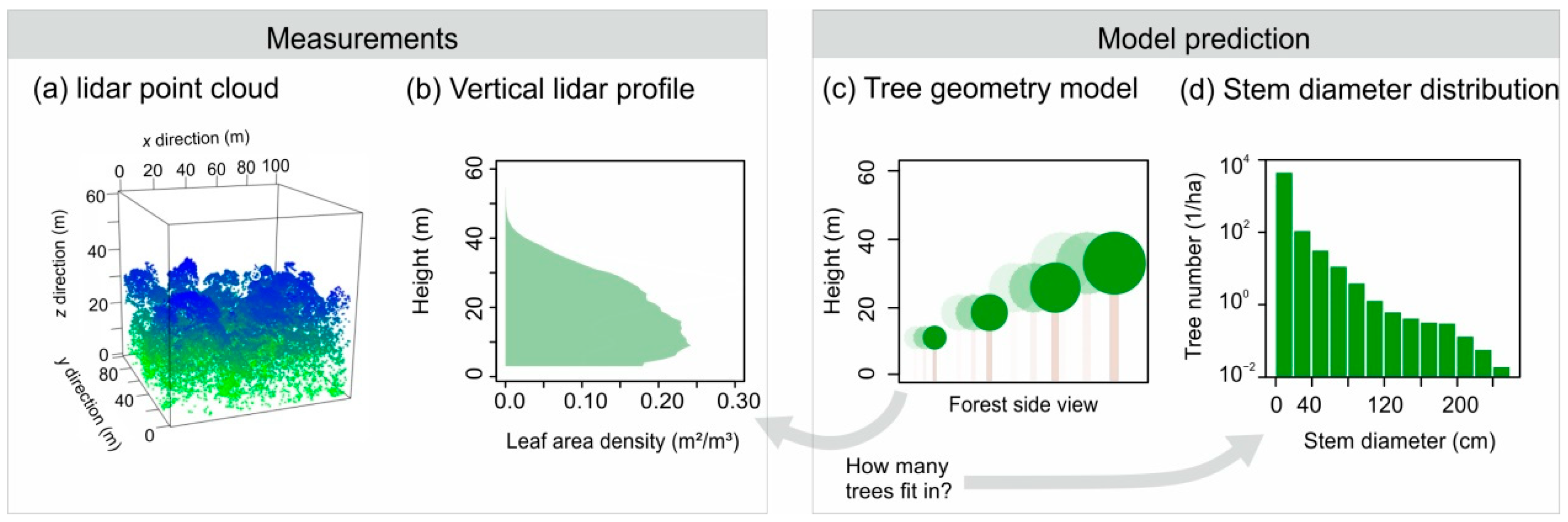
Combination of light detection and ranging (lidar) measurements with the tree geometry model to estimate the stem diameter distribution of a forest. The starting point is (a) the measured lidar point cloud (here shown for an exemplary 1 ha subplot of Barro Colorado Island (BCI)). Points are colored according to their height (with a gradient from the top with blue colors to the bottom with green colors). (b) The vertical leaf area profile can be derived from the lidar point cloud by accounting for decreasing lidar returns with decreasing height due to the tree leaf density (ground returns of height < 3 m are not shown). The vertical leaf area profile is then combined with the tree geometry model illustrated in (c). By calculating how many trees of specific size (illustrated by different shadings) can contribute tree crown leaves to the lidar -derived leaf area profile, we can estimate (d) the number of trees (per ha) in specific stem diameter classes (here, logarithmic y-axis, 50 ha plot of BCI, 20 cm diameter class width). See methods for details.
Figure 1.
Combination of light detection and ranging (lidar) measurements with the tree geometry model to estimate the stem diameter distribution of a forest. The starting point is (a) the measured lidar point cloud (here shown for an exemplary 1 ha subplot of Barro Colorado Island (BCI)). Points are colored according to their height (with a gradient from the top with blue colors to the bottom with green colors). (b) The vertical leaf area profile can be derived from the lidar point cloud by accounting for decreasing lidar returns with decreasing height due to the tree leaf density (ground returns of height < 3 m are not shown). The vertical leaf area profile is then combined with the tree geometry model illustrated in (c). By calculating how many trees of specific size (illustrated by different shadings) can contribute tree crown leaves to the lidar -derived leaf area profile, we can estimate (d) the number of trees (per ha) in specific stem diameter classes (here, logarithmic y-axis, 50 ha plot of BCI, 20 cm diameter class width). See methods for details.

Figure 2.
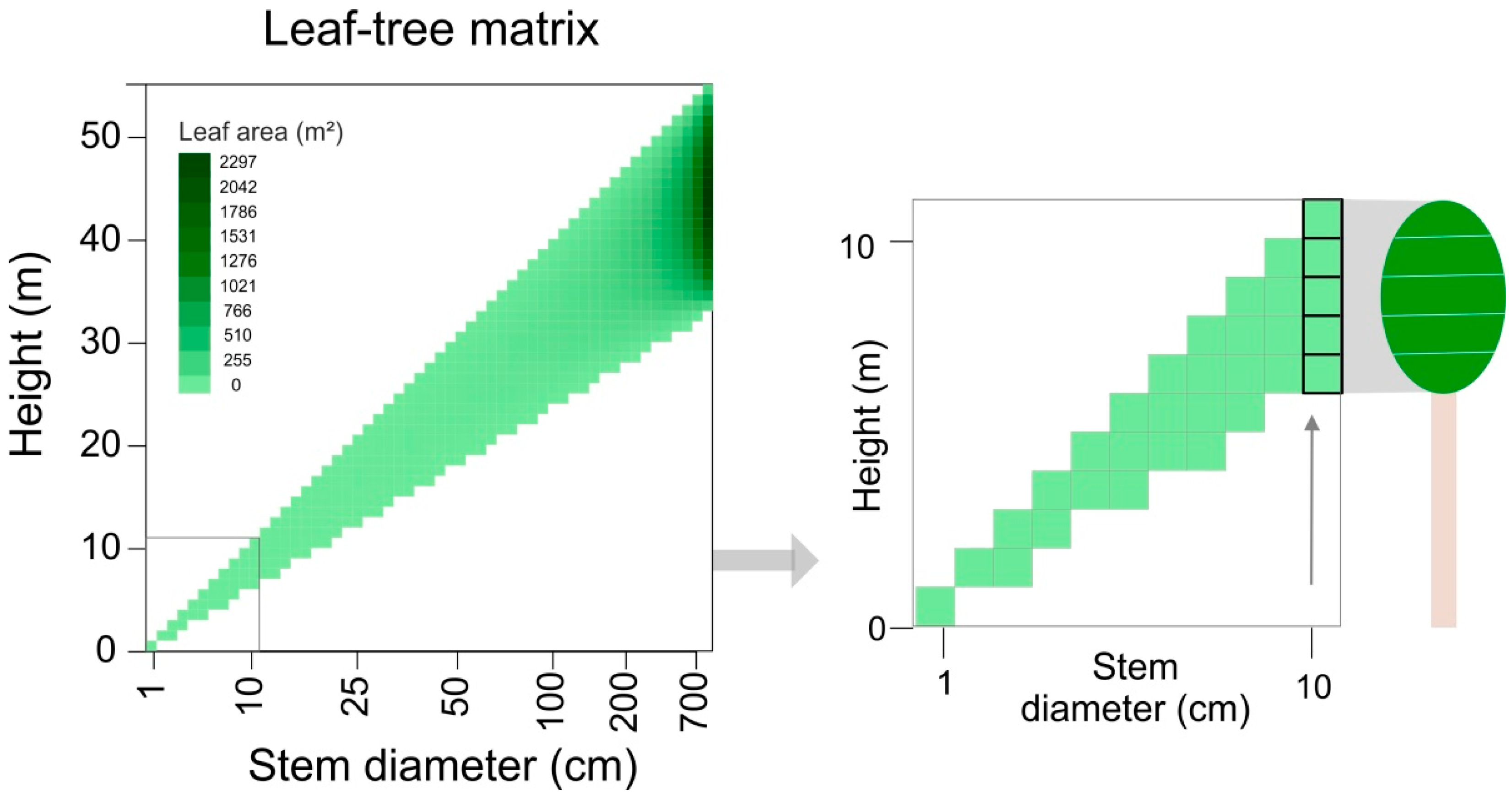
Visualization of the leaf–tree matrix (left) and an enlarged cut-out (right). Each column in the matrix reflects the leaf area contribution of one tree to different height layers. Columns represent different stem diameter classes. Colors in the matrix show leaf area values with a gradient from light green (low values) to dark green (high values) (white indicating no leaf area). On the right, an exemplary tree of 10 cm stem diameter is highlighted in the cut-out with its crown leaf area distributed to four height layers. Note the logarithmic x-axis of the stem diameter (cm).
Figure 2.
Visualization of the leaf–tree matrix (left) and an enlarged cut-out (right). Each column in the matrix reflects the leaf area contribution of one tree to different height layers. Columns represent different stem diameter classes. Colors in the matrix show leaf area values with a gradient from light green (low values) to dark green (high values) (white indicating no leaf area). On the right, an exemplary tree of 10 cm stem diameter is highlighted in the cut-out with its crown leaf area distributed to four height layers. Note the logarithmic x-axis of the stem diameter (cm).

Figure 3.
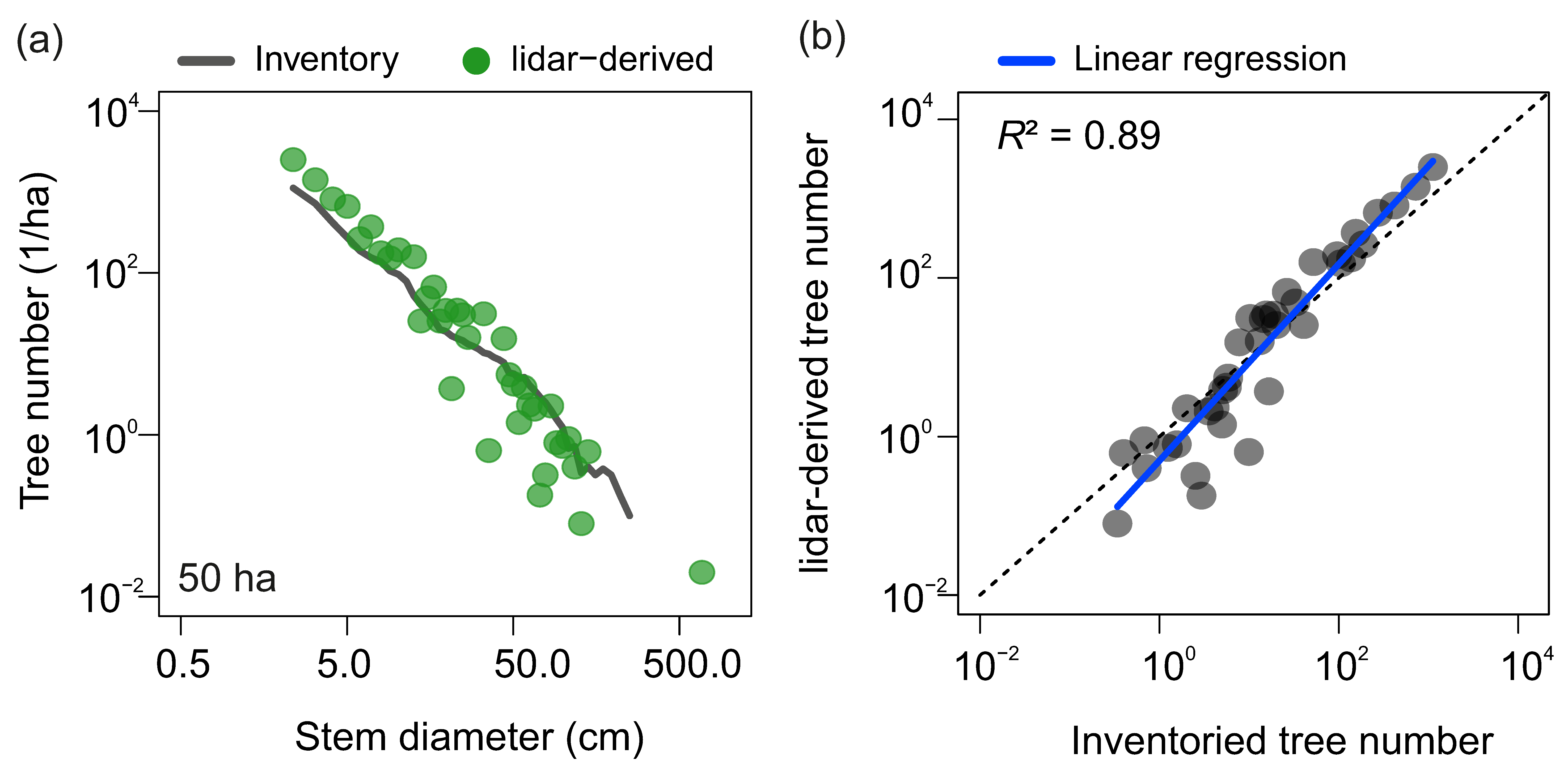
Comparison of the stem diameter distribution derived from lidar with field data at BCI (50 ha). (a) The tree number per stem diameter class derived from lidar (green points) and field inventory (grey line) of BCI on log–log axes (see methods for details). (b) 1:1 plot of the comparison on log–log axes including a linear regression line (blue line) for evaluation. Grey dots represent the logarithmic tree numbers for each stem diameter class comparing those derived from lidar (y-axis) and those censused in the inventory (x-axis). For the root mean square error (RMSE) (22.8 trees per ha) and normalized RMSE (nRMSE) (6.2%) values, we refer to the methods and Table 3.
Figure 3.
Comparison of the stem diameter distribution derived from lidar with field data at BCI (50 ha). (a) The tree number per stem diameter class derived from lidar (green points) and field inventory (grey line) of BCI on log–log axes (see methods for details). (b) 1:1 plot of the comparison on log–log axes including a linear regression line (blue line) for evaluation. Grey dots represent the logarithmic tree numbers for each stem diameter class comparing those derived from lidar (y-axis) and those censused in the inventory (x-axis). For the root mean square error (RMSE) (22.8 trees per ha) and normalized RMSE (nRMSE) (6.2%) values, we refer to the methods and Table 3.

Figure 4.
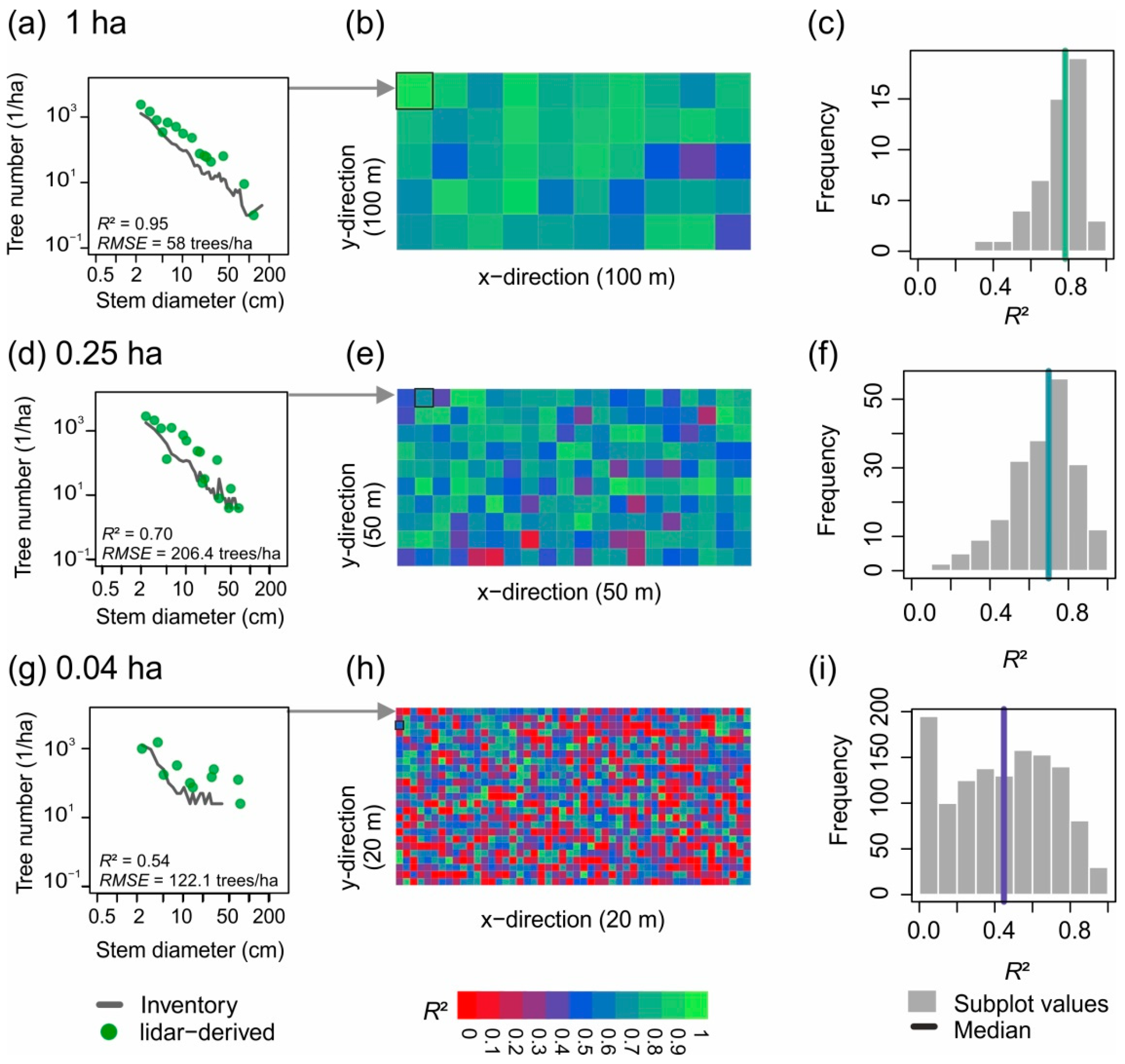
Stem diameter distributions derived from lidar for scales of 1, 0.25, and 0.04 ha. (a) An exemplary 1-ha plot of the BCI forest is illustrated by comparing the stem diameter distribution from inventory (grey line) with that derived from lidar (green points). (b) Map of BCI divided in 1-ha subplots and colored according to R² values. Values close to one (green) show a good estimation. The exemplary plot shown in (a) is highlighted with a black border. (c) Histogram of R² values for all subplots of 1 ha (the vertical line shows the median). Similar analysis is shown in (d–f) for the 0.25-ha scale and in (g–i) for the 0.04-ha scale. An analysis of the regression slope, RMSE and nRMSE values is shown in Table 3 and Figure A4.
Figure 4.
Stem diameter distributions derived from lidar for scales of 1, 0.25, and 0.04 ha. (a) An exemplary 1-ha plot of the BCI forest is illustrated by comparing the stem diameter distribution from inventory (grey line) with that derived from lidar (green points). (b) Map of BCI divided in 1-ha subplots and colored according to R² values. Values close to one (green) show a good estimation. The exemplary plot shown in (a) is highlighted with a black border. (c) Histogram of R² values for all subplots of 1 ha (the vertical line shows the median). Similar analysis is shown in (d–f) for the 0.25-ha scale and in (g–i) for the 0.04-ha scale. An analysis of the regression slope, RMSE and nRMSE values is shown in Table 3 and Figure A4.

Figure 5.
Scaling relations between plot size and goodness-of-fit measures. (a) The RMSE between lidar-derived and inventory-based stem numbers of subplots is shown (mean: black dots, standard deviation: grey polygon) with increasing plot size (ha). Please note the log–log axes. A linear regression (black line, based on black dots) provides a slope and R² of the respective scaling relation. A similar analysis is given for (b) nRMSE (%), (c) the regression slope of lidar-derived and inventory-based stem numbers, and (d) coefficient of determination R². Please note the different sample sizes for the different spatial scales (see also Table 3 and Table A2 for details).

Figure 6.
Comparison of lidar-derived and inventory-based (a–c) tree density (N) and (d–f) basal area (BA) for the (a,d) 1-ha scale, (b,e) 0.25-ha scale, and (c,f) 0.04-ha scale. Each black dot represents one subplot of the respective spatial scale. Dotted lines denote the 1:1 line. Blue lines show the linear regression line (with its equation and R² shown in each panel). Values on the bias, RMSE, and nRMSE are provided in Table 3. Please note the different axis ranges and sample sizes for the different spatial scales (see also Table 3).

Figure 7.
Correlations of R² with characteristics of the lidar profile, forest attributes, and profile differences. In (a) correlations of R² values and the mean profile height (WMPH) is shown at the 0.04-ha (left), 0.25-ha (middle) and 1-ha scale (right). Each black dot represents a forest plot, and the blue dashed lines reflect the optimal values for R² (close to one). The correlation coefficients are displayed below (Spearman’s r). In (b,c) the correlation coefficients are shown for each plot size: in (b) lidar-derived attributes (black: profile height WMPH, green: variance of leaf density) and in (c) forest attributes (black: tree density for d ≥ 1 cm, green: standard deviation of tree height). Grey dashed vertical lines show no dependence (r = 0).

Table 1.
List of attributes used for the correlations with R² (from the comparison of the estimated stem diameter distribution with field data). Columns denote the data used, a description of the attribute, its unit and the different statistical calculations applied.
Table 1.
List of attributes used for the correlations with R² (from the comparison of the estimated stem diameter distribution with field data). Columns denote the data used, a description of the attribute, its unit and the different statistical calculations applied.
| Data Source | Attribute | Unit | Calculations |
|---|---|---|---|
| lidar data | Profile height | m | Maximum, Median, Variance |
| Leaf area density | m²/m³ | Maximum, Median, Variance | |
| Number of lidar returns | 1/m2 | - | |
| profile height weighted by leaf area | m | Median (WMPH 1), Variance (WVPH 2) | |
| Forest inventory | Basal area 3,4 | m²/ha | Sum |
| Tree density 3,4 | 1/m2 | Sum | |
| Tree height 3 | m | Median, Standard deviation |
1 Median height of the vertical leaf profile derived from lidar (weighted by the derived leaf area density LADlidar per height layer). 2 Variance of height of the vertical leaf profile derived from lidar (weighted by the derived leaf area density LADlidar per height layer). 3 Including trees of stem diameter d ≥ 1 cm. 4 Including trees of stem diameter d ≥ 10 cm.
Table 2.
Sensitivity analysis of different model assumptions (see also Figure A2). The changed model assumptions for each scenario are written in bold.
Table 2.
Sensitivity analysis of different model assumptions (see also Figure A2). The changed model assumptions for each scenario are written in bold.
| Sensitivity Scenario | 1 | 2 | 3 | 4 |
|---|---|---|---|---|
| Crown shape | Sphere | Cylinder | Ellipsoid | Ellipsoid |
| Height allometry | Asymptotic | Asymptotic | Asymptotic | Power law |
| Crown length | Crown radius | 0.4 × height | 0.4 × height | 0.4 × height |
| Crown leaf density | 0.44 m²/m³ | 0.44 m²/m³ | 1 m²/m³ | 0.44 m²/m³ |
| Regression slope | 1.22 | 1.29 | 1.21 | 1.1 |
| R² | 0.89 | 0.98 | 0.92 | 0.89 |
| RMSE (trees/ha) | 32.0 | 4.5 | 15.0 | 15.3 |
| nRMSE (%) | 8.8 | 1.2 | 4.1 | 3.8 |
Table 3.
Comparison of forest attributes derived from lidar and from the forest inventory for different plot sizes. Results are shown for the regression analysis (slope and R²), RMSE and nRMSE (overall and for three different categories of small, mid-sized and large trees grouped according to stem diameter d) and aggregated forest attributes (tree density and basal area, for stem diameter d ≥ 10 cm). For each plot size, the mean ± standard deviation (and in brackets, minimum and maximum) of the respective attribute is given. The plot size is given in ha with the number of plots and plot dimension in m × m. Forest attributes are compared between lidar and inventory also in terms of the bias, RMSE, and nRMSE (%) (see methods for details). See Table A2 for additionally analyzed plot sizes.
| Plot Size (ha) | 50 | 1 | 0.25 | 0.04 | |
|---|---|---|---|---|---|
| Side length (m) in x-direction | 1000 | 100 | 50 | 20 | |
| Side length (m) in y-direction | 500 | 100 | 50 | 20 | |
| Number of plots | 1 | 50 | 200 | 1250 | |
| Overall quality | Regression slope | 1.24 | 0.9 ± 0.14 (0.66, 1.23) | 0.76 ± 0.2 (0.11, 1.3) | 0.55 ± 0.38 (−0.94, 2.17) |
| R² | 0.89 | 0.76 ± 0.13 (0.38, 0.95) | 0.67 ± 0.17 (0.13, 0.94) | 0.44 ± 0.27 (0.00005, 1) | |
| RMSE (trees/ha) | 22.8 | 67.6 ± 45.1 (15.2, 187.4) | 118.1 ± 77.6 (13.4, 385.6) | 219.2 ± 160.4 (17.7, 1074.6) | |
| nRMSE (%) | 6.2 | 18.8 ± 13.2 (4.2, 55.0) | 33.2 ± 21.7 (3.0, 105.7) | 70.9 ± 62.0 (3.2, 590.1) | |
| RMSE per size group (trees/ha) | Small trees 1 | 590.5 | 719.5 ± 379.6 (188.6, 1844.9) | 796.8 ± 492.6 (153.6, 3028.1) | 902.2 ± 751.6 (128.4, 5423.6) |
| Mid-sized trees 2 | 39.4 | 77.1 ± 30.5 (28.0, 175.3) | 112.9 ± 43.1 (39.9, 267.6) | 153.9 ± 73.9 (33.5, 606.7) | |
| Large trees 3 | 1.2 | 5.1 ± 2.5 (2.2, 15.9) | 9.1 ± 5.5 (2.4, 36.1) | 26.2 ± 21.2 (0, 230.3) | |
| Tree density 4 (trees/ha) | Inventory-based | 447.3 | 447.3 ± 46.1 (353, 597) | 447.3 ± 60.4 (300, 648) | 447.3 ± 115.7 (175, 1025) |
| lidar-derived | 516.7 | 615.5 ± 159.3 (364, 1320) | 758.9 ± 249.2 (316, 1864) | 992.6 ± 402.5 (150, 3125) | |
| bias | −69.4 | −168.2 | −311.6 | −545.3 | |
| RMSE | 69.4 | 228.4 | 394.4 | 677.8 | |
| nRMSE (%) | 15.5 | 51.1 | 88.2 | 151.5 | |
| Basal area 4 (m²/ha) | Inventory-based | 30.1 | 30.1 ± 5.1 (20.4, 45.8) | 30.1 ± 8.3 (15.5, 67.9) | 30.1 ± 20.9 (3.5, 206.1) |
| lidar-derived | 23.6 | 29.3 ± 6.9 (18.8, 58.1) | 38.1 ± 15.0 (9.5, 163.4) | 59.0 ± 45.0 (4.7, 762.5) | |
| bias | 6.5 | 0.8 | −8.0 | −28.9 | |
| RMSE | 6.5 | 4.7 | 14.3 | 49.8 | |
| nRMSE (%) | 21.6 | 15.7 | 47.4 | 165.3 | |
1 Stem diameter classes d ≤ 10 cm. 2 Stem diameter classes 10 cm < d ≤ 50 cm. 3 Stem diameter classes d > 50 cm. 4 Stem diameter classes d ≥ 10 cm.
Publisher’s Note: MDPI stays neutral with regard to jurisdictional claims in published maps and institutional affiliations. |
© 2021 by the authors. Licensee MDPI, Basel, Switzerland. This article is an open access article distributed under the terms and conditions of the Creative Commons Attribution (CC BY) license (http://creativecommons.org/licenses/by/4.0/).
Share and Cite
MDPI and ACS Style
Taubert, F.; Fischer, R.; Knapp, N.; Huth, A. Deriving Tree Size Distributions of Tropical Forests from Lidar. Remote Sens. 2021, 13, 131. https://0-doi-org.brum.beds.ac.uk/10.3390/rs13010131
AMA Style
Taubert F, Fischer R, Knapp N, Huth A. Deriving Tree Size Distributions of Tropical Forests from Lidar. Remote Sensing. 2021; 13(1):131. https://0-doi-org.brum.beds.ac.uk/10.3390/rs13010131
Chicago/Turabian StyleTaubert, Franziska, Rico Fischer, Nikolai Knapp, and Andreas Huth. 2021. "Deriving Tree Size Distributions of Tropical Forests from Lidar" Remote Sensing 13, no. 1: 131. https://0-doi-org.brum.beds.ac.uk/10.3390/rs13010131
Note that from the first issue of 2016, this journal uses article numbers instead of page numbers. See further details here.