A Genetic Optimization Resampling Based Particle Filtering Algorithm for Indoor Target Tracking


1
International Doctoral Innovation Center, University of Nottingham Ningbo China, Ningbo 315100, China
2
Department of Land Surveying and Geo-Informatics, The Hong Kong Polytechnic University, Hong Kong, China
3
School of Computer Science, University of Nottingham Ningbo China, Ningbo 315100, China
4
Nottingham Geospatial Institute, University of Nottingham, Nottingham NG7 2RD, UK
*
Author to whom correspondence should be addressed.
Remote Sens. 2021, 13(1), 132; https://0-doi-org.brum.beds.ac.uk/10.3390/rs13010132
Submission received: 30 November 2020
/
Revised: 20 December 2020
/
Accepted: 30 December 2020
/
Published: 2 January 2021
(This article belongs to the Special Issue Indoor Localization)
Abstract
:In indoor target tracking based on wireless sensor networks, the particle filtering algorithm has been widely used because of its outstanding performance in coping with highly non-linear problems. Resampling is generally required to address the inherent particle degeneracy problem in the particle filter. However, traditional resampling methods cause the problem of particle impoverishment. This problem degrades positioning accuracy and robustness and sometimes may even result in filtering divergence and tracking failure. In order to mitigate the particle impoverishment and improve positioning accuracy, this paper proposes an improved genetic optimization based resampling method. This resampling method optimizes the distribution of resampled particles by the five operators, i.e., selection, roughening, classification, crossover, and mutation. The proposed resampling method is then integrated into the particle filtering framework to form a genetic optimization resampling based particle filtering (GORPF) algorithm. The performance of the GORPF algorithm is tested by a one-dimensional tracking simulation and a three-dimensional indoor tracking experiment. Both test results show that with the aid of the proposed resampling method, the GORPF has better robustness against particle impoverishment and achieves better positioning accuracy than several existing target tracking algorithms. Moreover, the GORPF algorithm owns an affordable computation load for real-time applications.
1. Introduction
Indoor target tracking (i.e., dynamic positioning) based on wireless sensor networks (WSN) has received considerable attention in engineering and industrial fields in recent years [1]. The applications include product tracking in logistics, automated guided vehicles (AGV) tracking in indoor industrial scenarios, and process monitoring in car smart-manufacturing factories, etc. As one of the mathematical methods used in indoor target tracking, the Bayesian filter (a.k.a. Bayesian estimation) estimates the target position by combining the position estimation at the previous time step with the known specific system motion model and the latest measurements. Kalman filter (KF) is a well-known estimation method in the Bayesian framework, but it can only deal with the linear problems with Gaussian models. For the tracking problems, which are generally with non-linear state-space models, two variants of KF called extended Kalman filter (EKF) [2] and unscented Kalman filter (UKF) [3] are used instead. Some research on using EKF and UKF in target tracking is described in [4,5,6]. However, these two estimation methods have some limitations. For example, both of them have difficulties in dealing with the problems with non-Gaussian models. Moreover, they require known prior information of the initial position, which is usually difficult to obtain in practice [6].
Another effective estimation method in the Bayesian framework is particle filter [7]. Its key idea is to approximate the required posterior distribution of target position by a set of discrete independent random particles (samples) with associated weights [6]. Similar to the other estimation methods in the Bayesian framework (including EKF and UKF), particle filter recursively performs position estimation through two important phases, i.e., prediction and update. In the prediction phase, the particles are propagated to the next time step using the specific system motion model, and a set of predicted particles are generated. Then in the update phase, each predicted particle is evaluated by the latest measurements and assigned with importance weight. A particle filter is widely used for target tracking since it can perform global positioning (i.e., positioning when the initial position is unknown). Compared to the EKF and UKF, a particle filter can provide position estimations with higher accuracy in the highly non-linear problems with arbitrary distribution [8]. However, the particle filter still suffers from some problems. There are two main problems that significantly affect the performance of a particle filter in indoor target tracking, namely, the inaccuracy of the measurements and the particle impoverishment. The former problem generally results from the non-line-of-sight (NLOS) and multipath signals. A lot of research on this problem has been done in the past two decades and a series of solutions have been proposed [9,10,11,12,13]. In contrast, the research on particle impoverishment is still relatively limited. Comprehensive and exhaustive research on this problem is required.
Resampling is generally performed after the state estimation to tackle the inherent particle degeneracy problem in particle filtering algorithm [6]. Resampling aims to select and copy the particles with high weights and replace the ones with low weights. However, this operation will lead to the loss of particle diversity, also known as particle impoverishment. When the number of particles (i.e., sample size) used in the filter or the measurement noise of a dynamic system is small, this particle impoverishment becomes more serious [6,8]. The particle impoverishment degrades the positioning accuracy and robustness, sometimes it may even cause filtering divergence and tracking failure. In this sense, mitigating particle impoverishment in a particle filtering algorithm is crucial for accurate and robust indoor target tracking.
To date, some solutions to the particle impoverishment problem have been proposed. A simple solution is adding Gaussian jitter noise to the over-centralized resampled particles [14]. Besides, the regularized particle filter (RPF) proposed in [15] constructs a diffusion kernel density function for each particle before resampling to prevent particle impoverishment. However, both solutions above are ineffective in situations where the measurement noise or the number of particles is very small. In the resample-move sequential Markov chain Monte Carlo (RM-SMCMC) algorithm proposed in [16], the particle diversity is maintained by moving a resampled particle to a neighboring region according to a given acceptance probability. The drawback of this solution is that it requires substantial computation to run the algorithm until convergence. Moreover, the risk sensitive particle filter (RSPF) in [17] mitigates particle impoverishment by constructing explicit risk functions. Li et al. [18] propose a deterministic resampling method that can strictly keep the original state density and maintain particle diversity. In the recent decade, solutions based on genetic algorithms are widely used for improving the particle filter-based target tracking performance. Since it is indicated that the particle filter has similar implementation characteristics to that of a genetic algorithm [19,20], the evolutionary ideas can be introduced to the particle filter by treating the filtering problem as a sequential optimization problem. Park et al. [21] propose an evolutionary particle filter that uses the genetic algorithm-inspired proposal distribution for particle sampling. Zhang et al. [22] propose an evolutionary particle filter based on self-adaptive multi-features fusion. The genetic algorithm can be specifically used in the resampling phase and increases the diversity of particles [23]. Wang et al. [24] propose a genetic algorithm-based resampling method, in which the crossover and mutation probabilities used in the genetic operation are both determined adaptively according to the degree of particle degeneracy. Zhao and Li [25] use a particle swarm optimization (PSO) strategy in the resampling phase to shift the particles to the higher likelihood region. Moghaddasi and Faraji [26] propose an algorithm called reduced particle filter based upon genetic algorithm (RPFGA), where the particles with the highest weights are selected to perform evolution using a genetic algorithm in the resampling phase. Test results of the above solutions show that they can mitigate particle impoverishment and improve state estimation performance to some extent. However, most of these solutions have more complexity and suffer from higher computation load, which is a challenge for real-time applications. Moreover, few of these solutions take into account the quality of resampled particles and their effects on state estimation. Therefore, it is difficult to guarantee these solutions are still effective when the number of particles used in the filter is very small.
Aiming at mitigating the effect of particle impoverishment on positioning and improve the positioning accuracy, this paper proposes an improved genetic optimization based resampling method. The proposed resampling method consists of five operators, i.e., selection, roughening, classification, crossover, and mutation. This resampling method is then integrated into the particle filtering framework to form a genetic optimization resampling based particle filtering (GORPF) algorithm. The results of two different tracking tests show that with the aid of the proposed resampling method, the GORPF achieves significantly better positioning accuracy than several existing indoor target tracking algorithms with an affordable computation load for real-time applications. The contributions of this paper are listed as follows.
(1) The proposed improved genetic optimization based resampling method is able to optimize the distribution and maintain the diversity of the resampled particles, which is generally unavailable for the traditional resampling methods.
(2) The proposed GORPF algorithm can improve the positioning accuracy by about 25% when comparing with the state-of-the-art positioning algorithms. Moreover, it has strong robustness to the particle impoverishment resulted from a small number of particles and small measurement noise.
2. Materials and Methods
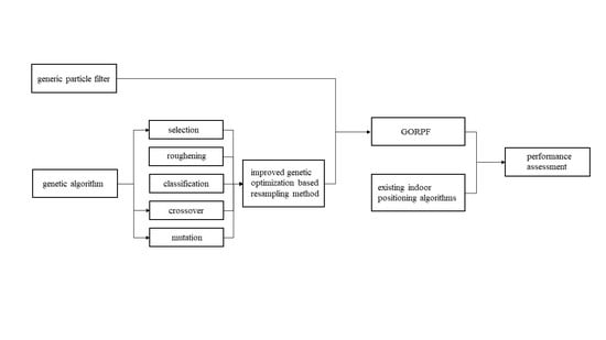
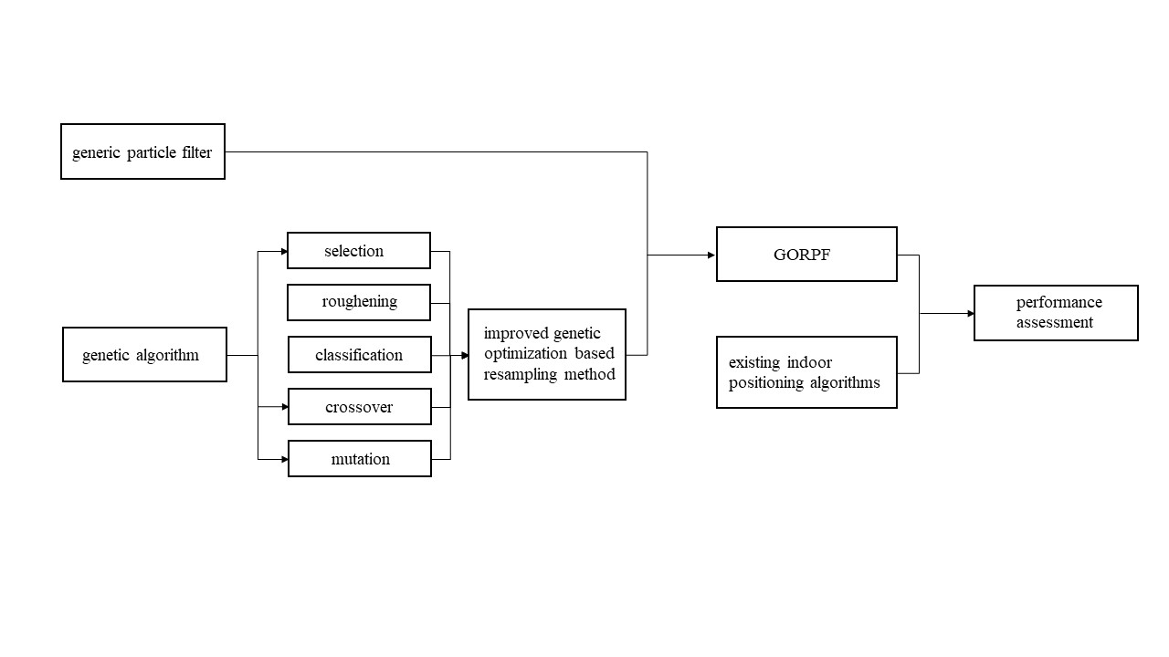
This section first briefly introduces the basics of the particle filter and genetic algorithm that were used in the algorithm development in this work. Inspired by the idea of a genetic algorithm, an improved genetic optimization resampling method was proposed. This proposed resampling method was integrated into the particle filtering framework to form a GORPF algorithm. The description of the proposed resampling method, as well as the full procedure of the GORPF algorithm, were presented. Finally, the performance assessment of the proposed GORPF algorithm in target tracking was carried out. Two different and independent tracking tests were described.
2.1. Basics of a Generic Particle Filter and Genetic Algorithm
This subsection first introduces the principle of a generic particle filter. Then, the concept of a genetic algorithm is briefly described.
2.1.1. Generic Particle Filter
A particle filter is a sequential Monte Carlo method in the framework of a Bayesian filter. Before the brief introduction of a generic particle filter, the state-space model of the dynamic system should be defined first. The state-space model aimed to find out the optimal state estimate given the observed data. A general form of the dynamic state-space model was defined as follows [6]
where and were the state vector and measurement vector at time step , respectively. and were the additive white process and measurement noise, respectively. The covariance of process noise and measurement noise denoted and , respectively. and were the two known transition and measurement functions, respectively, and they were probably non-linear. The particle filter assumed that the states subject to the first-order Markov process, and were conditionally independent given the states.
The particle filter approximated the posterior distribution of state by a set of particles that were randomly sampled from a known proposal distribution , given by
in which was the Dirac delta function, was the number of particles, and was the normalized importance weight (also called weight in the following) of the th particle. The weight (unnormalized) of the th particle at time step (i.e., ) could be updated by
The choice of the proposal distribution affected the state estimation performance. In practical applications, the transition distribution was usually used as the proposal distribution, i.e., . In this case, the weight update in Equation (4) was simplified as
The weights obtained from Equation (5) needed to be normalized before resampling. The weight normalization was given by
After a few of the iterations, all but a small number of particles would have negligible weights, this was the so-called particle degeneracy problem. This problem resulted in a lot of computation being wasted on updating the particles that had negligible contributions to the approximation of posterior distribution. The approximated effective sample size is usually used to measure the degree of particle degeneracy, which was given by
A small value indicated a severe particle degeneracy and vice versa. When a severe particle degeneracy was observed (i.e., was less than a manually predefined threshold ), resampling was implemented, otherwise, the posterior particles were directly used for the state prediction at the next time step. The above calculation was specifically designed for the generic particle filter. It was also available to perform resampling in every iteration without calculating , such as the sequential importance resampling (SIR) algorithm (a.k.a. bootstrap filter) [6]. SIR is the most widely used particle filter in practice.
2.1.2. Genetic Algorithm
The genetic algorithm is a population-based optimization method that simulates the natural biological evolution process. Every candidate solution in the solution space of the optimization problem corresponds to every individual in nature, and they are updated in every generation.
The traditional genetic algorithm requires an encoding operation before the update of the candidate solutions. Encoding is the process of representing a candidate solution in the form of a string that conveys the information, this process is similar to the formation of chromosomes in biology. Each bit in the string represents a piece of information in the candidate solution. One of the most widely used encoding methods is binary encoding, which represents a candidate solution with the strings of 0 and 1 [27]. This encoding method is usually used in knapsack problems [28]. Another more simple and straightforward encoding method is real-value encoding. It represents the candidate solution with a vector of real numbers. More details of the real-value encoding method can be found in [29].
The update of candidate solutions in the standard genetic algorithm is generally performed through three important operators, i.e., selection, crossover, and mutation. The selection operator selects the candidate solutions based on the law of “the survival of the fittest”—selecting good solutions and eliminating bad solutions while keeping the population size constant. The quality of a candidate solution is evaluated by the fitness function and quantified by the fitness value. This fitness value reflects how close the candidate solution is to the optimal solution. Some common selection methods in the genetic algorithm are introduced in [30]. The selected solutions are then inputted into the mating pool (i.e., a collection of the selected solutions), and they will be used in the following crossover operator. The crossover operator randomly selects two candidate solutions (i.e., parents) from the mating pool and exchanges part of their information to create new solutions (i.e., offspring). Some common crossover methods are introduced in [31]. Similar to individuals in nature, the mutation may happen on the offspring solutions in the genetic algorithm. The mutation operator is to change part of the information in the offspring solutions, this is important for maintaining population diversity and preventing the genetic algorithm trapping into local optimal solutions.
This paper introduced the idea of a genetic algorithm to the resampling phase. An improved genetic optimization resampling method was proposed. The introduction of this proposed resampling method is described in the next subsection.
2.2. Genetic Optimization Resampling-Based Particle Filter (GORPF)
In this subsection, the proposed improved genetic optimization resampling method is described first. Then, the procedure of the GORPF algorithm is presented.
2.2.1. Improved Genetic Optimization Resampling Method
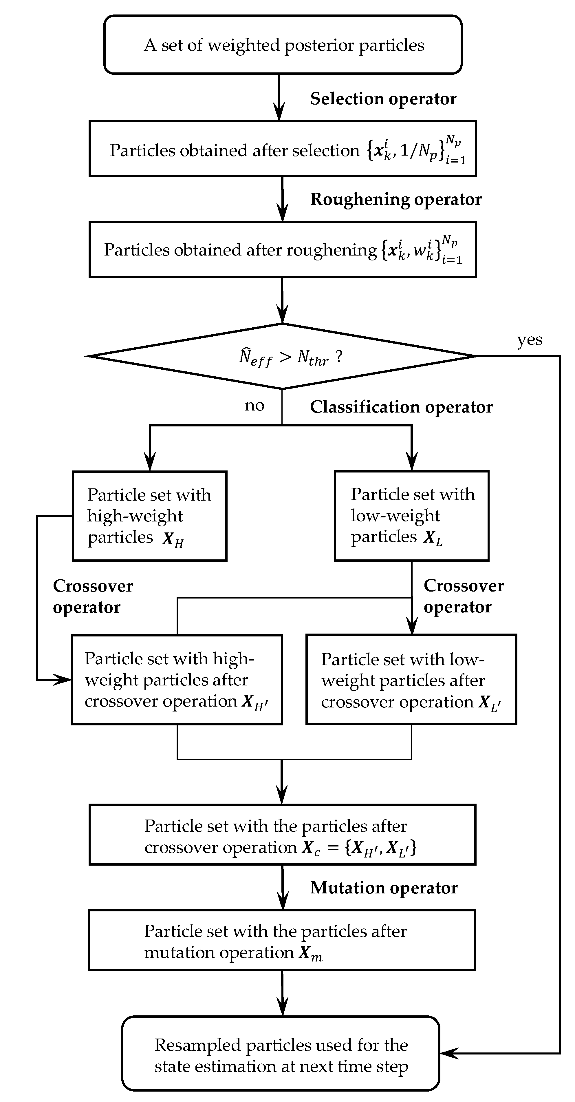
The improved genetic optimization resampling method was designed to mitigate the particle impoverishment problem and improve positioning accuracy. Before describing the proposed resampling method, the encoding method needed to be determined first. As aforementioned, binary encoding is widely used. However, this encoding method may not be appropriate for particle filter-based tracking problems. The particles used in the tracking problem consisted of a string of real numbers. When using the binary encoding method, each component in the particle (such as the position and velocity in this work) needs to be coded as a binary string to enable the selection, crossover, and mutation, and then each binary string requires to be decoded as a real number to calculate the goal function [32]. This process requires a high computation load, especially when the solution space of the problem is large. Besides, binary encoding is often not natural for many problems and sometimes corrections must be made after crossover and/or mutation [33]. In the target tracking problems based on a particle filter, each particle is essentially a candidate solution of the state estimation that contains a vector of real numbers. These real numbers can be the coordinates, velocity, acceleration, heading angle, etc. of the target. Compared to the binary encoding method, the real-value encoding method can characterize these particles more accurately and has a lower computation load. Therefore, the real-value encoding method was used directly in the proposed genetic optimization resampling method. A flowchart of the proposed resampling method is given in Figure 1. The proposed resampling method contained five operators, i.e., selection, roughening, classification, crossover, and mutation. Each operator in the method is described as follows.
Selection
Consider that a set of normalized weighed particles are obtained and formulated as , where is the particle and is the weight. is the total number of particles. Taking the computation complexity and quality of the selected particles into consideration, the Roulette wheel selection [34] method was used. The probability of a particle to be selected was proportional to its weight in this method. The steps of the Roulette wheel selection are described as follows.
(1) Sorting the particles in descending order according to the weights and create a cumulative weight table as
(2) Randomly generate random numbers from the standard uniform distribution .
(3) For each random number , the th particle is selected if
The above selection operation is equivalent to the traditional simple random resampling. The high-weight particles are selected and copied, and those low-weight ones are eliminated. However, the particles obtained from Equation (9) suffered from particle impoverishment due to the multiple copies of a few high-weight particles. Moreover, the particles remained may trap into the local optimal regions. In our proposed resampling method, these selected particles needed to be optimized (by the operators described in the following) before they could be used for the state estimation at the next time step. This was different from the traditional simple random resampling method which uses the resampled particles for the state estimation at the next time step directly. The weights of the selected particles were reset to .
Roughening
The diversity of the particles obtained from the selection operator were seriously reduced. In order to increase the diversity of these particles, a simple roughening operator was implemented by adding a random zero-mean Gaussian jitter noise to each particle. This jitter noise assumed that each component in the particle (i.e., state vector) was independent, thus its covariance matrix was a diagonal matrix. For a particular component in the particle, its standard deviation was given by
where was the difference between the maximum and minimum values of this component among all the particles (before roughening), was the dimension of the state vector, was a constant tuning parameter which affects the magnitude of jitter noise, and was the total number of particles. The magnitude of the jitter noise significantly affected the particle distribution after roughening. A too-large jitter noise would result in very dispersive particles. This may cause particle degeneracy since some of the dispersed particles may fall into the solution regions that have negligible contributions to the state estimation. A too-small jitter noise would cause tight clusters of points to be distributed around the original particles. As a result, the roughening operation tended to be ineffective for particle impoverishment mitigation. Therefore, the tuning parameter should be determined carefully, and its determination method can be found in [14]. In order to improve the robustness of the resampling method, it was necessary to evaluate the quality of the particles after roughening. The weight of each particle was recalculated by Equation (5). Since the original particles (i.e., the particles obtained in selection operator) had the same weights (i.e., ), the weights of the particles after the roughening operation were proportional to their measurement likelihood values, i.e., . These particles as well as their normalized weights were then input to the mating pool.
Classification
As aforementioned, the particle degeneracy may happen when the tuning parameter was not set properly. For the purpose of evaluating the degeneracy degree of the particles obtained after roughening, the approximated effective sample size was calculated according to Equation (7). If was greater than the predefined threshold , these particles could be used in the state estimation at the next time step directly without the additional operations. Otherwise, a particle classification was performed as follows.
(1) Sorting the particles in descending order according to their weights as
where was the mating pool that contains particles obtained from roughening operation. denoted the sorted particle and its normalized weight.
(2) Finding out the integer which satisfies
(3) Classifying the sorted particles in into two disjoint particle sets as
in which denoted the particle set containing high-weight particles, and denoted the particle set containing low-weight particles. The integer was the boundary between the high-weight and low-weight particles. This classification reflected the quality of each particle.
Crossover
Crossover is performed to increase the diversity of particles and avoid the particles trapping into the local optimal solutions. In this paper, the parental particles in the two different particle sets in Equation (13) implemented the crossover operation with different rules. Note that the fitness of a particle is determined by the measurement likelihood function in this paper, i.e., , where was the fitness of particle . measured the goodness of fit (i.e., the degree of similarity) of a particle to the measurement. The crossover operations for the particles in the two different particle sets are described as follows.
For the crossover operation of the particles in , particle pairs were generated by randomly selecting two different parental particles and from first. Each particle in could only be selected once. If in (12) was an even number, particle pairs could be generated. If was an odd number, particle pairs could be generated, the only one particle left did not implement a crossover operation and it remained unchanged in . The fitness values of and were and , respectively. Each particle pair was applied to the arithmetic crossover [35] with a probability . The arithmetic crossover was an interpolating linear combination of the two particles. With the arithmetic crossover, two offspring particles, and , could be calculated by
where and were the weighting factors determined by
The fitness of the two offspring particles was calculated and denoted as fitness and , respectively. The crossover probability was determined adaptively using the Sigmoid function [36] in neural networks, which was given by [37]
in which , were the predefined empirical upper and lower bounds of crossover possibility. was a determined coefficient with the value of 9.903438. and are the maximum and average fitness values of the parental particles in , respectively. wais the larger fitness value of the two selected parental particles, i.e., . The offspring particles and obtained by Equation (14) were accepted based on the Metropolis rule [38]. This rule accepts the degraded offspring particle with a certain probability. If was greater than , was accepted. Otherwise, was accepted with the probability of . This was implemented by generating a random number from a standard uniform distribution and comparing it with . If , was accepted, otherwise, it is rejected. The accepted replaced its parental particle in , otherwise remained unchanged in . This Metropolis rule was also applied for . The crossover operation above was repeated until all the particle pairs were implemented. After the crossover operation, the particle set was re-denoted as . The fitness values of the particles in the were recalculated. Different to the traditional genetic algorithms, in which the crossover probability is a predefined constant, the crossover probability used here was adaptively determined according to the fitness of every particle in . When the particles had the risk of suffering from premature convergence to the local optimal solution (i.e., was close to ), it increased the values of crossover probability; when the particles had the risk of suffering from divergency in the solution space (i.e., was close to ), it decreased the values of crossover probability. This adaptive crossover probability could improve the robustness to against premature convergence and divergence.
For the crossover operation of the particles in , a modified arithmetic crossover operator was designed. Each particle in implemented the crossover with another parental particle selected from , and their offspring particle was calculated by
in which was the parental particle from , and was the parental particle selected (using the Roulette wheel selection method according to the fitness values) from . was a random weighting factor which was drawn from the uniform distribution [0, ], where was the upper bound of . The value of at a certain time step could be calculated as
where was the total number of particles, and was the approximated effective sample size calculated by Equation (7). characterized how much information from was transmitted to the offspring particle . The smaller the value of , the more information was transmitted. The offspring particle replaced its parental particle in . After the crossover operation, the particle set was re-denoted as . The fitness values of the particles in the were recalculated. Different to the arithmetic crossover operator used for the particles in , this modified arithmetic crossover operator was only implemented on the low-weight particle from , and only one offspring particle was generated. For the parental particle from , it did not generate offspring particles. This modified arithmetic crossover operator could modify the low-weight particles into high-weight ones while the modified particles would not overlap the high-weight particles. This could shift the particles to the region of the global optimal solution and maintain the diversity of particles.
Mutation
Redefine as the combination of and , i.e., . For each particle in , the mutation was performed with a probability , given by
where was the particle obtained after mutation operation, and its fitness was calculated and denoted as . was the particle drawn from . was a zero-mean Gaussian distributed random variable with the covariance . The mutation probability was determined adaptively using the Sigmoid function, which was given by [37]
where , were the predefined empirical upper and lower bounds of mutation possibility. was the coefficient whose value was 9.903438. was the fitness of the particle . and were the maximum fitness and average fitness of the parental particles in , respectively. The particles obtained by Equation (19) was accepted based on the Metropolis rule. If was greater than , was accepted. Otherwise, was accepted with the probability of . The accepted replaced its parental particle in , otherwise remained unchanged in . The mutation operation above was repeated until particles were obtained. After the mutation operation, the particle set was re-denoted as . Similar to the characteristics of crossover probability in Equation (16), the adaptive mutation probability here could maintain the diversity of the particles while ensuring stable convergency. After performing the five operators in the improved genetic optimization resampling, each particle was treated equally. The weights of the particles were reset to .
2.2.2. Genetic Optimization Resampling-Based Particle Filter
The GORPF algorithm was proposed by integrating the improved genetic optimization based resampling method into the particle filtering framework. In the proposed GORPF, the transition distribution was used as the proposal distribution and hence the weights of the particles could be updated according to Equations (5) and (6). Once the weighted particles were obtained, the state at the time step could be estimated using the weighted sum of the particles, given by
where denoted the state estimated by the GORPF algorithm, and denoted the state and corresponding weight of the th particle, respectively. After the state estimation, the proposed resampling was performed. The resampled particles were then used in the state estimation at the next time step. The full procedure of the proposed GORPF algorithm is presented in Table 1.
2.3. Assessment of the Proposed Method
This subsection describes the performance assessment of the proposed GORPF algorithm in target tracking. Two different and independent tracking tests were carried out. The first test was assessing the proposed algorithm in a one-dimensional tracking problem with a univariate growth model [21] through a simulation, and the second test was assessing the proposed algorithm in a three-dimensional tracking problem with a constant velocity motion model [8] through an experiment. In both tests, the positioning performance of the proposed GORPF algorithm was compared to the four state-of-the-art tracking algorithms in the literature, i.e., SIR [6], SIR with Gaussian jitter noise (SIR-GJN) [14], IGPF [24], and RPFGA [26]. The five particle filter-based algorithms (including the GORPF algorithm) use different strategies to mitigate the particle impoverishment and different methods to determine the parameters needed in genetic operation. Among the five algorithms, the SIR does not use any strategy for particle impoverishment mitigation. The SIR-GJN uses the roughening strategy, the RPFGA, IGPF, and GORPF use strategies based on genetic algorithms. The parameters needed in the genetic operation in the RPFGA algorithm are predefined constants while these parameters are adaptively determined in the IGPF and GORPF algorithms.
The data processing in both Test A (simulation) and Test B (experiment) were performed in the same computer system and software. The system configuration and software version are given in Table 2.
2.3.1. Test A: One-Dimensional Tracking
A one-dimensional target tracking problem with a univariate growth model was considered in this test. This model is highly non-linear, multimodal, and nonstationary, and it is widely used to assess the performance of estimation methods. The state-space model in this problem was formulated as
where and represented the mutually independent Gaussian process and measurement noises, respectively. In the test, the variance of the process noise was set to . The particle impoverishment was related to the magnitude of measurement noise and particle number used in the filter. In order to evaluate the robustness of the algorithms to these two factors, the variance of the measurement noise in this test was set to two different values (i.e., for normal measurement noise and for small measurement noise), and the particle number was set to two different values (i.e., 100 and 20). was the position that needed to be estimated, the initial position was and its variance was set to 1. The initial particles were generated from the Gaussian distribution, i.e., . In this test, the true position of the target, as well as the measurement at each time step, were simulated based on the state-space model in Equations (22) and (23) beforehand. The units of position and time step was meter and second, respectively.
Regarding the parameters (, , , and ) in the GORPF algorithm, they were determined by tuning the parameters around the values provided by [22]. The parameters and used for crossover probability determination in Equation (16) were set to 0.9 and 0.6, respectively, and the parameters and used for mutation probability determination in Equation (20) were set to 0.1 and 0.01, respectively. Our proposed method generally had optimal performance with the above parameter settings. The variance for generating the random number in the mutation operator was set to the same value as the variance of process noise. The threshold was set to . For an unbiassed assessment, the above parameters used for the genetic operation were also used in the RPFGA and IGPF algorithms unless some parameters could be determined adaptively. The position estimation started at the time step and finished at the time step . Each algorithm obtained 50 position estimations which corresponded to the 50 time steps. The test was repeatedly performed 20 times (different runs with different seeds) and the mean values were used to represent the positioning results. Root mean square error (RMSE) was used as the positioning accuracy assessment metric in this test, given by
where was the total number of time steps (i.e., 50). was the time step from 1 to . and were the estimated and “truth” positions at time step , respectively.
2.3.2. Test B: Three-Dimensional Tracking
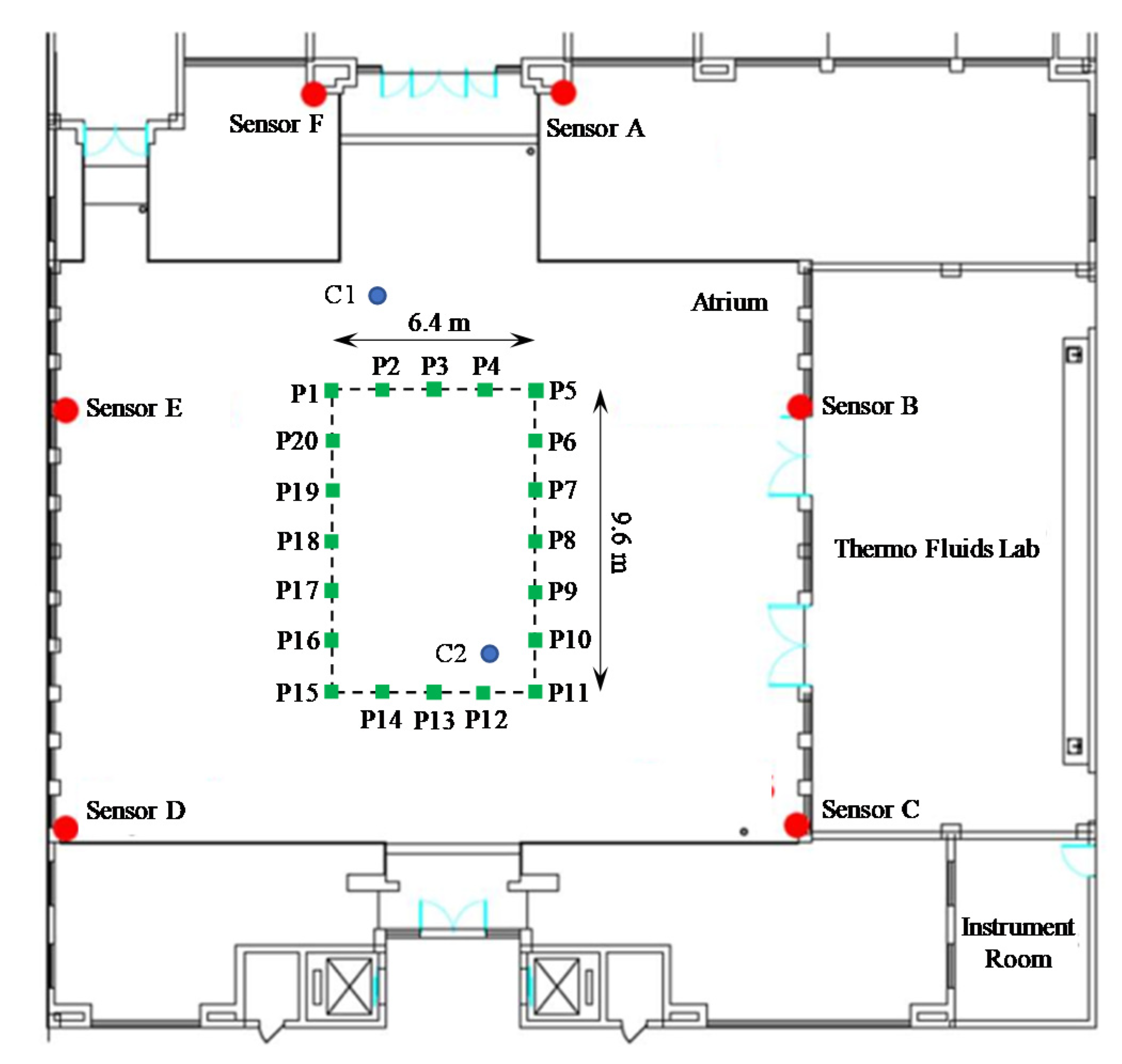
A three-dimensional target tracking problem with a constant velocity model was considered in this test. The test was performed in the atrium of the Sir Peter Mansfield Building at the University of Nottingham Ningbo China (UNNC). There were six ultrawideband (UWB) sensors installed on the wall of the building. Compared to the traditional wireless positioning techniques (such as WiFi), UWB transmits information based on a non-sinusoidal narrow pulse (nanosecond-level), but not carrier phase, over a wide portion of the frequency spectrum [4]. Inherently, the extremely high time resolution, as well as the large bandwidth of UWB, enables it to have the advantages such as high ranging accuracy, high penetrating power [39], less interference from multipath effect [40], high-speed data transmission [41], etc. Therefore, UWB sensors were used to generate the measurements required for target position estimation in this test.
A closed traverse survey was carried out before the test to obtain the coordinates of the UWB sensors in the Universal Transverse Mercator (UTM) reference system. The closed traverse involved four stations, and the total length was 104.697 m. The angular misclosure and linear misclosure of the traverse were 17.5′′ and 4.48 mm, respectively. The fractional linear misclosure was 1 in 23370. A leveling survey was carried out to determine the normal heights of the traversing stations. The leveling involved three instrument points. The misclosure of leveling was 1 mm. The coordinates of the two traversing stations in the atrium, i.e., C1 and C2 (see Figure 2), were determined through traverse and leveling. To minimize the errors in traverse and leveling propagating into the coordinates of UWB sensors, the coordinates of the six UWB sensors were determined through the total station survey from C1 and C2. The calculations of the traverse were performed by a MicroSurvey software called Star*Net. The basics of the traverse, leveling, and total station survey can be found in [42].
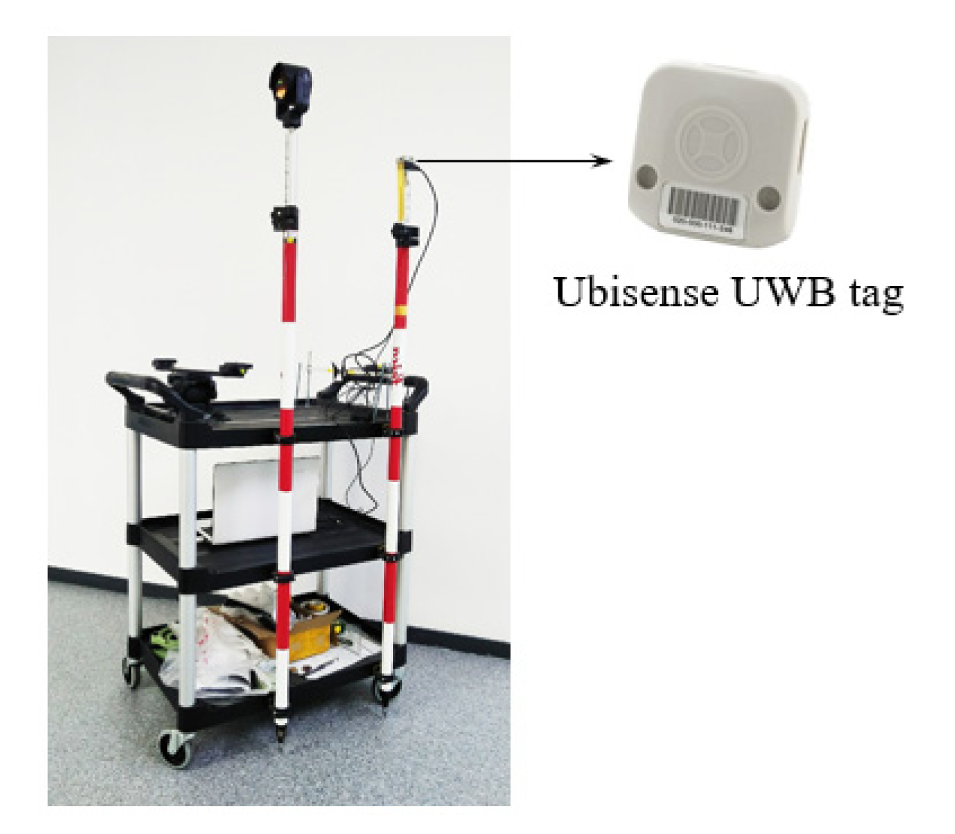
A trolley was used in this test. As shown in Figure 3, two ranging rods were tightly attached to the trolley, and a UWB tag was fixed on the top of a ranging rod. A rectangular track with the size of 9.6 m × 6.4 m was set in the middle of the atrium. The trolley and track helped to obtain the well-controlled tag position and height for the algorithm validation. Twenty test points with an interval of 1.6 m were distributed on the rectangular track (see Figure 2). These test points were used for the positioning accuracy assessment. The horizontal coordinates of all the test points were known by the total station survey from C1 and C2, and the heights of the test points were determined by the leveling survey. The UWB measurements were collected by moving the trolley between the twenty test points with a stop-and-go method. The stop-and-go method meant to start the trolley at rest at a test point and move towards and stop at the next test point for five seconds. When the trolley stopped, the measurements at that point could be used to estimate the position, and this position estimate was compared with the “truth” for evaluation purposes. This rigorous stop-and-go test allowed us to get the UWB measurements at each test point accurately because it was free from the effect of residual in UWB time synchronization, dynamics of the moving trolley platform, and the accuracy of visiting test points at a particular time. In our measurement collection, the trolley started from the test point P1, it moved steadily on the track in the clockwise direction and stopped (with the tip of the ranging rod pointed at the known test point on the track) at each test point in turn. Finally, the trolley moved back to P1.
The state-space model of the 3-D tracking problem in this test was defined as follows. We defined the state vector of the target as , in which was the 3-D position and was the 3-D velocity. A random-walk model was used as the state model without loss of generality, which was given by [8]
where
and was the sampling interval. was the zero-mean Gaussian random process noise with known covariance . This state model assumed that the velocity was subject to an unknown acceleration which was characterized by the motion process noise.
The UWB system used in the test provided both time-of-arrival (TOA) and angle-of-arrival (AOA) measurements. TOA was the signal travel time between tag and sensor, this travel time could be converted to a range measurement by multiplying the travel time with the speed of light. AOA was based on the direction of incidence from which the received signal arrived. For 3-D positioning, the AOA measurements contained azimuth and elevation measurements. It was indicated that the positioning method using both range and angle measurements could improve the positioning accuracy and robustness [43]. Therefore, both TOA and AOA measurements were used in the test. Since six UWB sensors were used in the test, the measurement vector consisted of eighteen measurements, i.e., , where was the range (derived from TOA), azimuth, and elevation measurement of the th sensor, respectively. The UWB TOA and AOA measurement models can be found in [44]. The measurement noises of TOA, azimuth, and elevation are mutually independent, their standard deviations were denoted as , and , respectively.
The parameters used in this test are summarized in Table 3. Since the number of particles used affected the positioning accuracy of the particle filter-based algorithm, we performed tuning and found that the accuracy tended to be stable when 2000 particles were used in each algorithm. After that, an increase in the particle number did provide significant accuracy improvement in each algorithm. This was because the prior densities enabled the predicted particles to be distributed closer to the mean of the posterior densities. Therefore, 2000 particles were used in each particle filter-based algorithm in this test. The crossover and mutation probabilities used in this test were the same as those in Test A. The covariance of process noise (i.e., ) was determined by tuning. The variance of the process noise in each direction was assumed to be the same in this test, i.e., , where was the variance of the process noise in the three directions. The standard deviations of the measurement noise were determined by statistical method. The parameter in the mutation operation in this test could be expressed as , where was the variance of the random variable added to the position component and was the variance of the random variable added to the velocity component. For an unbiased assessment, the above genetic parameters used in the GORPF algorithm were also used in the RPFGA and IGPF algorithms unless some parameters could be determined adaptively. EKF is another positioning algorithm in the Bayesian framework which is widely used for three-dimensional target tracking problem because of its high positioning accuracy [4]. For the purpose of verifying the three-dimensional positioning performance of EKF, it was included in the assessment along with the five particle filter-based algorithms. The test was repeatedly performed 20 times (different runs with different seeds) and the mean values were used to represent the positioning results. The positioning accuracy was assessed by comparing the coordinates of the twenty test points determined by each algorithm with the “truth” that was determined by the total station survey. The mean radial spherical error (MRSE) was used as the assessment metric for evaluating the positioning accuracy in 3-D space
where was the number of test points, was the samples from 1 to . , and were the estimated easting, northing, and height, respectively of sample . , and were the “truth” coordinates determined by the total station survey. In addition to the positioning accuracy, computation load is another important metric that requires to be assessed in three-dimensional target tracking problems. The averaged computation time required for positioning at a point was used as the assessment metric of computation load. The computation time of the particle filter-based algorithm was dependent on the number of particles used. Since the particle number was set to 2000 in each particle filter-based algorithm, this computation load assessment was unbiased. The computation time was determined through the function of “tic” and “toc” in MATLAB.
3. Results
This section presents the results of the two tracking tests. The results of Test A and Test B are presented in Section 3.1 and Section 3.2, respectively.
3.1. Results of Test A
The RMSEs of the five algorithms (i.e., SIR, SIR-GJN, RPFGA, IGPF, and GORPF) in the different test conditions (different particle numbers and different magnitudes of measurement noise) are presented in Table 4. Moreover, the tracking trajectories as well as the absolute errors of the five algorithms in the different test conditions are shown in Figure 4, Figure 5 and Figure 6.
3.2. Results of Test B
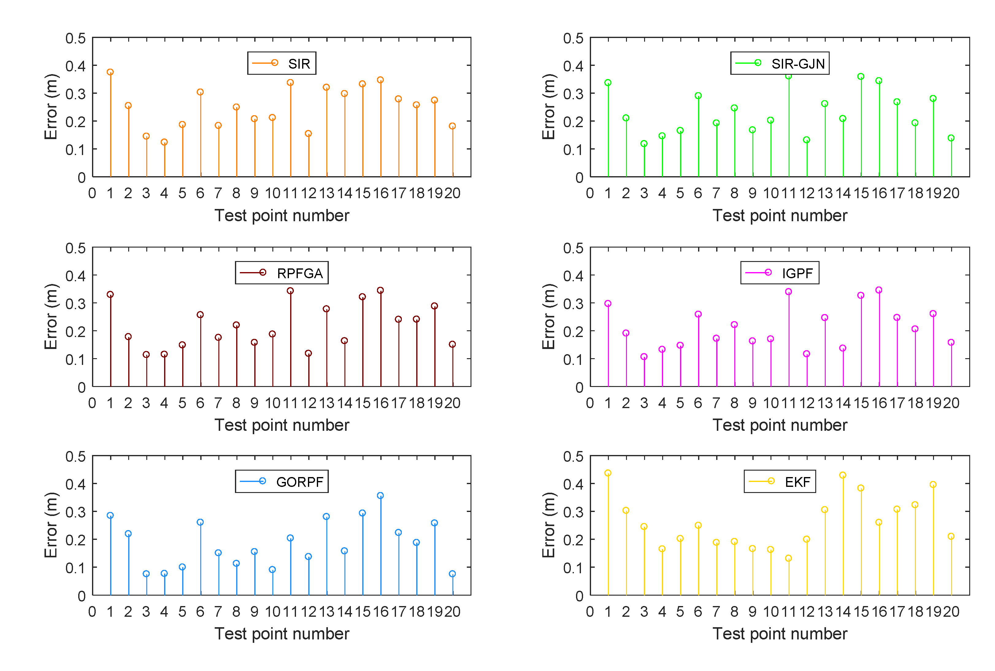
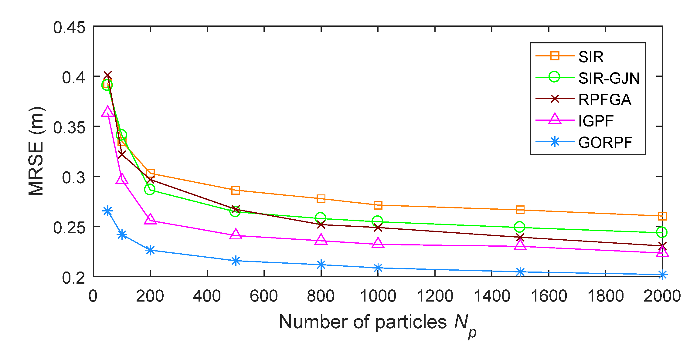
The MRSEs and computation time of the six algorithms (the five particle filter-based algorithms and the EKF algorithm) are shown in Table 5. The positioning errors of each algorithm at the twenty test points are presented in Figure 7. Note that the results in Table 5 are based on the condition that sufficient particles (i.e., 2000) are used. In order to evaluate the robustness of each algorithm on the particle number, we set the value of to eight different numbers (i.e., 50, 100, 200, 500, 800, 1000, 1500, 2000). The MRSEs of each algorithm with respect to the particle number are shown in Figure 8.
4. Discussion
This section discusses the test results presented in Section 3. The results of the two tests are discussed separately first. The future research direction is then briefly discussed.
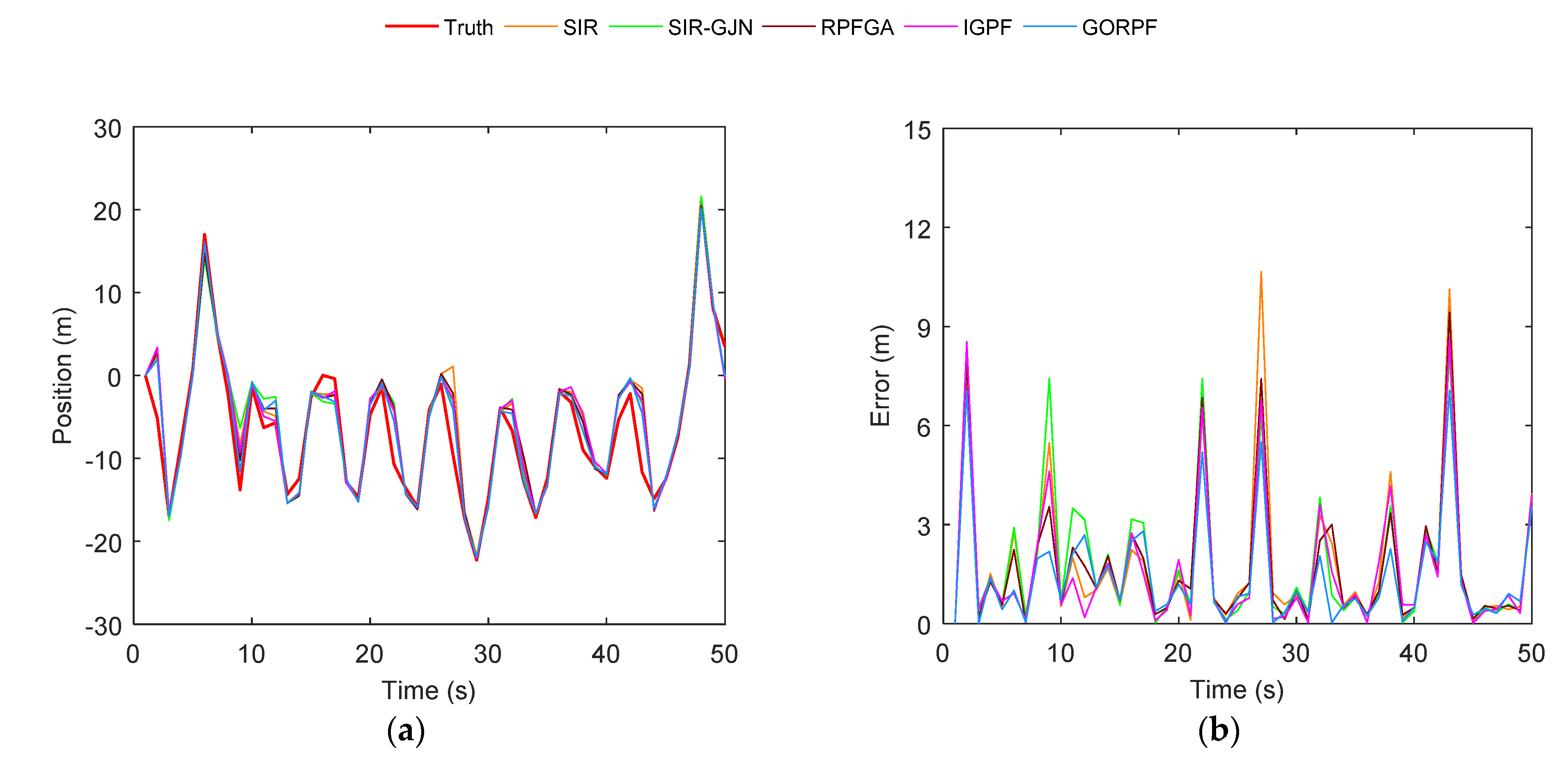
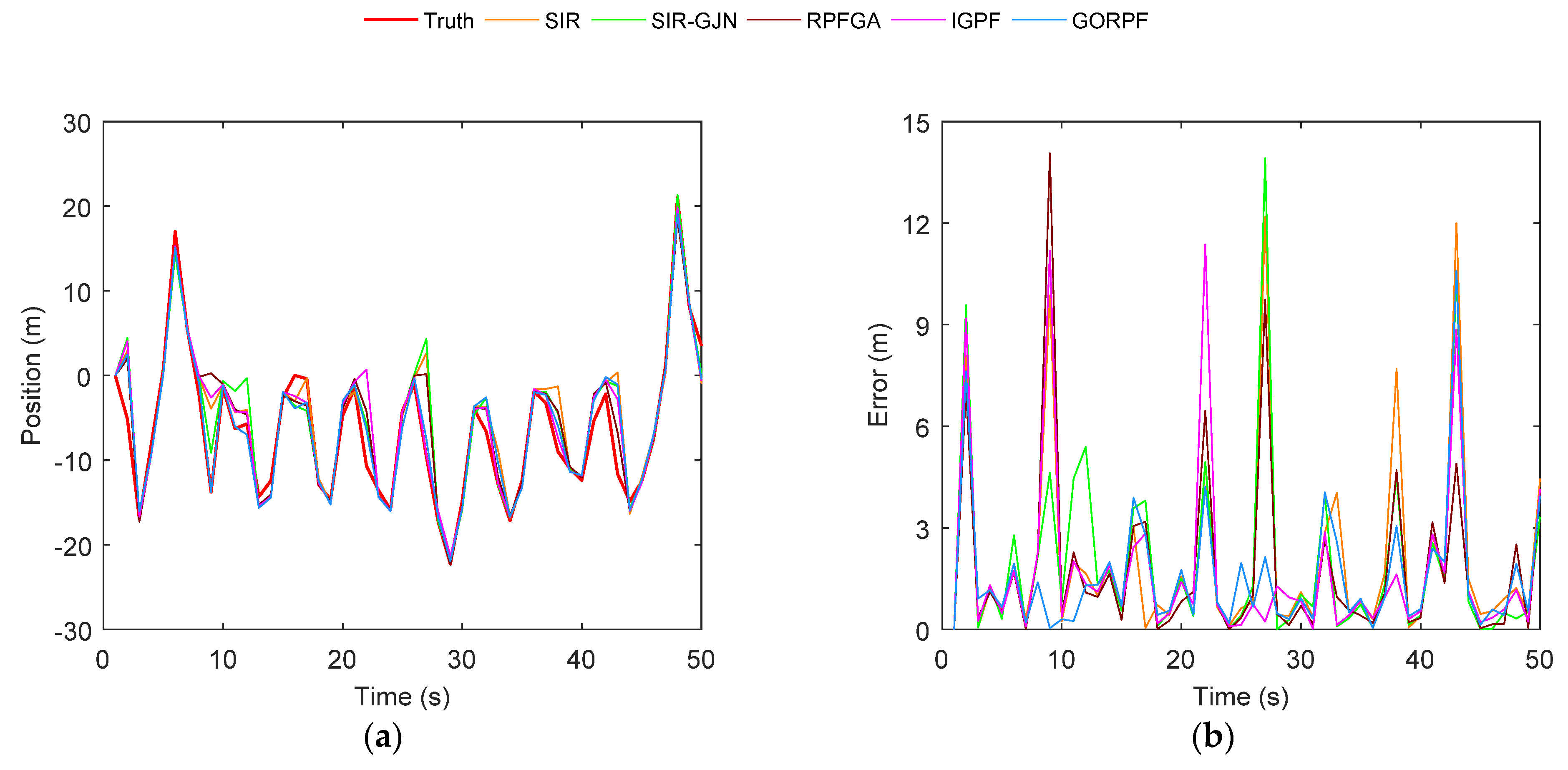
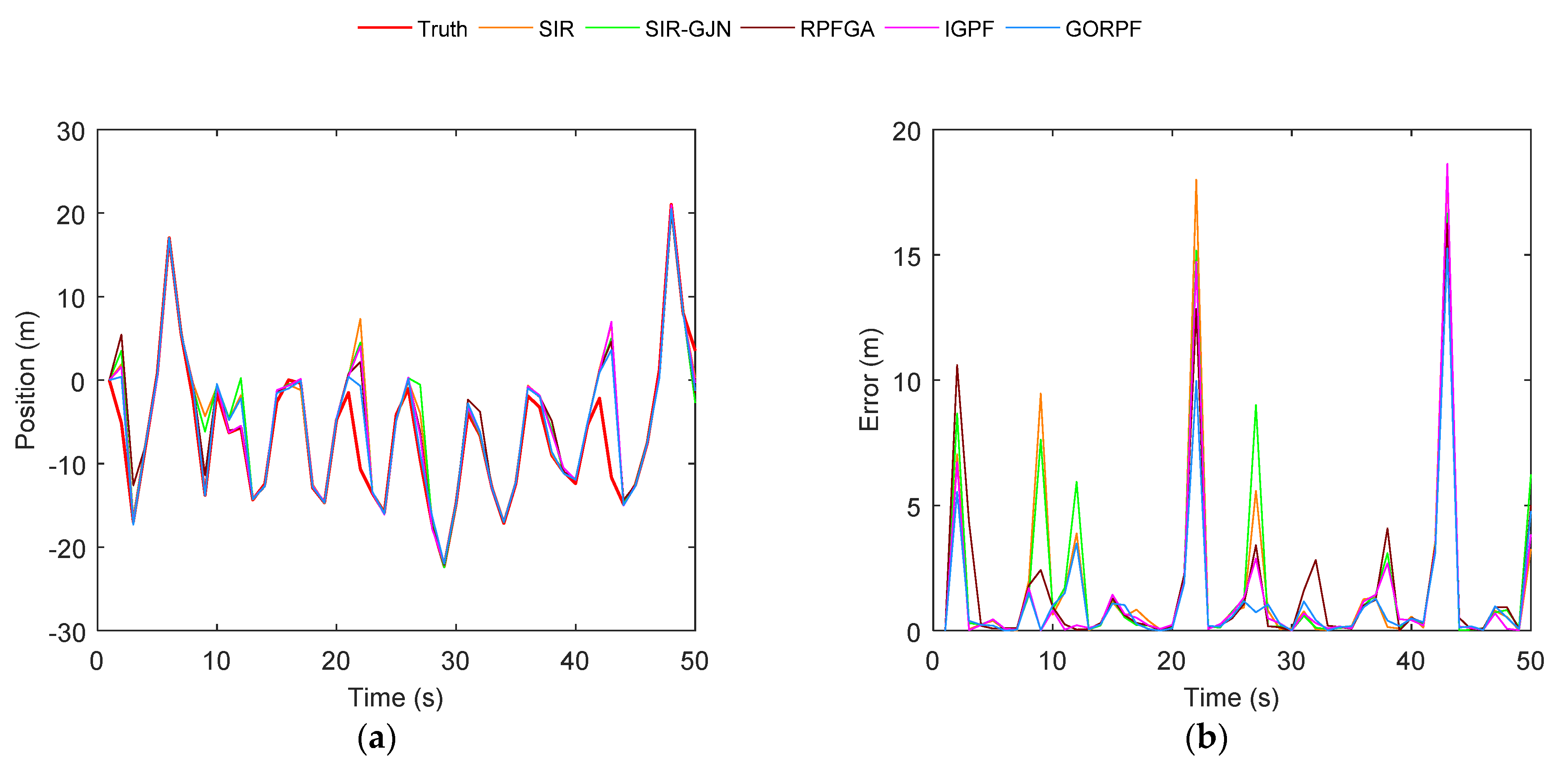
Regarding Test A, as the SIR algorithm does not use any strategy for particle impoverishment mitigation, it is used as the baseline for performance comparison. The results in Table 4 show that with the same particle number and measurement noise magnitude, the four algorithms with the strategies for particle impoverishment mitigation (called algorithms with strategies in the following) outperform the SIR algorithm. Among these four algorithms with strategies, the GORPF algorithm performs best. Compared to the SIR algorithm, the GORPF algorithm improves the positioning accuracy by about 29.4% on average while SIR-GJN, RPFGA, and IGPF improve the accuracy by about 3.65%, 11.02%, and 12.05% on average, respectively. Considering the effect of particle number and measurement noise magnitude on positioning, we found that decreasing the values of these two parameters will lead to the positioning accuracy reduction. Specifically, by comparing Test 1 with Test 2 (both tests use the same magnitude of measurement noise but a different number of particles), it is found that decreasing the particle number from 100 to 20 results in the positioning accuracy reductions of the five particle filter-based algorithms. This can be also reflected by comparing Figure 4 to Figure 5 which demonstrates that the positioning errors in Figure 5 are generally larger than those in Figure 4. Insufficient particles cannot accurately represent the posterior distribution and also increase the degree of particle impoverishment. Moreover, it increases the risk of suffering from premature convergence to the local optimal solution. Table 4 shows that the four algorithms with strategies can always outperform SIR even though the particle number used is decreased. This reveals that the strategies used in these four algorithms are all effective in maintaining particle diversity and improving positioning accuracy. However, when taking the extent of accuracy reduction into account, Table 4 shows the accuracy of SIR-GJN decreases by about 21.4%, which is the largest among the four algorithms with strategies. The comparison between Figure 4 and Figure 5 shows that the SIR-GJN algorithm has significantly larger errors at some time steps than those of the other three algorithms with strategies. This implies that using roughening alone for the mitigation of particle impoverishment (caused by a small number of particles) is less effective than the strategies used in the other three algorithms (i.e., RPFGA, IGPF, and GORPF). Table 4 shows that the accuracy of the GORPF is decreased by about 12.8%, which is the least among the four algorithms with strategies. This implies the proposed resampling method used in the GORPF algorithm has the best performance on maintaining particle diversity and improving positioning accuracy. When comparing Test 1 with Test 3 (both tests use the same number of particles but different measurement noise), it is found that decreasing the covariance of measurement noise from 1.0 to 0.04 results in the positioning accuracy reduction of the five particle filter-based algorithms. This can be also reflected by comparing Figure 4 to Figure 6 which shows that the positioning errors in Figure 6 are significantly larger than those in Figure 4. The small measurement noise implies that the likelihood function concentrates in a small region of the state space, the predicted particles obtained by the dynamic model in the prediction phase tend to locate at the tail of likelihood function [45]. This can cause particle impoverishment, and hence the position estimation accuracy will be significantly decreased. The four algorithms with strategies outperform SIR under the small measurement noise condition, which reveals the effectiveness of the strategies used in these four algorithms. Again, taking the extent of accuracy reduction into account, it shows that both the accuracies of the GORPF and RPFGA algorithms are decreased by about 33.1% while those of the other three algorithms are decreased by about 40%. This implies that the strategies used in the GORPF and RPFGA algorithms have a better effect on the mitigation of particle impoverishment (caused by small measurement noise) than the strategies used in the other two algorithms (i.e., SIR-GJN and IGPF). Based on the discussions above, comprehensively, the proposed GORPF algorithm has better robustness against particle impoverishment (caused by small measurement noise and a small number of particles) and achieves better positioning accuracy than the other four algorithms.
Regarding Test B, both the SIR algorithm and the EKF algorithm do not use any strategy to mitigate particle impoverishment. The positioning accuracy of the two algorithms is similar. The results in Table 5 shows that the RMSE difference is only 7.4 mm. Figure 7 shows the maximum error of the EKF algorithm (about 0.45 m) is slightly larger than that of the SIR algorithm (about 0.4 m). However, the difference in computation time between them is very large. EKF requires almost 8 times longer time than that of SIR for position estimation at a point. This is because EKF requires calculation of the Jacobian matrix at each time step. The Jacobian matrix calculation is very time-consuming in large dimensional problems, such as the case in the tracking problem in Test B where the dimension of the measurement vector was eighteen. Regarding the five particle filter-based algorithms, when taking the SIR algorithm (without particle impoverishment mitigation strategy) as a baseline, the other four algorithms all achieve improved positioning accuracies. Table 5 shows that the GORPF algorithm performs best in terms of positioning accuracy among them. Compared to the SIR algorithm, the GORPF algorithm improves positioning accuracy by about 22.4%. Figure 7 shows that the maximum error of the GORPF algorithm is about 0.35 m and the minimum error is less than 0.1 m. Both values are less than those in the other five algorithms. As shown in Figure 8, the number of particles does affect the positioning accuracy of each particle filter-based algorithm. Increasing the particle number will improve the positioning accuracy of each algorithm. When insufficient particles are used in the filtering (such as is less than 200), the positioning accuracy will reduce significantly. Nevertheless, the SIR-GJN, RPFGA, IGPF, and GORPF algorithms can generally outperform the SIR algorithm because of their strategies used for particle impoverishment mitigation. This finding agrees with the finding in Test A. A very small number of particles can cause a serious loss of particle diversity. Figure 8 shows that when only 50 particles are used in each algorithm, the positioning accuracy of the GORPF is much higher than those of the other four algorithms (which are almost 0.4 m). This reveals the GORPF has better robustness to particle impoverishment than the others. The outstanding performance of the GORPF mainly owes to the improved genetic optimization resampling method used. Different from the Gaussian jitter noise roughening operation which is used alone in the SIR-GJN algorithm, our proposed resampling method implements a genetic operation based on the particles obtained from the roughening operation. This genetic operation can avoid the particles falling into the region of the local optimal solution and make the particles distribute in the region of the global optimal solution. Moreover, with the aid of the classification operation used in the proposed resampling method, the low-weight particles can be modified into high-weight particles. This classification operation improves the “quality” of the offspring particles and hence improve the positioning robustness. Therefore, the GORPF algorithm performs better in terms of positioning accuracy than the RPFGA and IGPF algorithm (both of them do not implement the classification operation). As for the computation time, the differences between the five particle filter-based algorithms are large. SIR requires the shortest computation time. Since the SIR-GJN, RPFGA, IGPF, and GORPF algorithms use different strategies (i.e., Gaussian jitter noise or/and genetic operators) for particle impoverishment mitigation, these added extra strategies directly result in a higher computation load than the SIR. Although the proposed GORPF algorithm requires the longest computation time (0.3382 s), such computation time is affordable for most real-time indoor tracking applications.
As discussed above, the GORPF has a relatively high computation load because of the added extra strategy for particle impoverishment mitigation. This is also the problem in many other genetic algorithm based particle filters, such as [46] and [47]. Although improving the computer system configuration is an effective way for improving computation efficiency, it will increase the cost. Therefore, decreasing the computation load by optimizing the algorithm itself (such as reduce computation steps and optimize the logic) may be a research direction for the genetic algorithm-based particle filter in the future.
5. Conclusions
This paper proposes an improved genetic optimization resampling method which consists of five operators, i.e., selection, roughening, classification, crossover, and mutation. The proposed resampling method is integrated into the particle filtering framework to form a genetic optimization resampling based particle filtering (GORPF) algorithm. The proposed algorithm is assessed by a one-dimensional tracking simulation test and a three-dimensional tracking experiment. The results in both tests show that the GORPF algorithm achieves better positioning accuracy than the state-of-the-art indoor positioning algorithms in the literature, even if the particle number and measurement noise magnitude are small. The proposed novel resampling method in the GORPF algorithm can effectively address the particle degeneracy, maintain the particle diversity, and improve the positioning accuracy and robustness. Moreover, the computation time of the GORPF algorithm is affordable for most real-time tracking applications. The improved positioning accuracy and robustness as well as the relatively low computation load of the GORPF algorithm make it possible to be used in people tracking in airports, object tracking in logistics, and machine guidance in Industry 4.0.
Author Contributions
Conceptualization: N.Z. and L.L.; Data curation: N.Z.; Formal analysis: N.Z. and R.B.; Investigation: N.Z., R.B., and T.M.; Methodology: N.Z. and L.L.; Software: N.Z.; Validation: N.Z. and T.M.; Visualization: N.Z.; Writing—Original draft: N.Z.; Writing—review and editing: L.L., R.B., and T.M.; Supervision: L.L., R.B., and T.M.; Funding acquisition, project administration and resources: L.L. All authors have read and agreed to the published version of the manuscript.
Funding
This work is financially supported by the International Doctoral Innovation Centre, Ningbo Education Bureau, Ningbo Science and Technology Bureau, and the University of Nottingham. This work was also supported by the UK Engineering and Physical Sciences Research Council under grant EP/L015463/1, and the Zhejiang Natural Science Foundation (ZJNSF) General Programme under grant LY17D040001.
Institutional Review Board Statement
Not applicable.
Informed Consent Statement
Not applicable.
Data Availability Statement
Data sharing is not applicable to this article.
Conflicts of Interest
The authors declare no conflict of interest. The founding sponsors had no role in the design of the study; in the collection, analyses, or interpretation of data; in the writing of the manuscript, and in the decision to publish the results.
References
- Khan, D.; Ullah, S.; Nabi, S. A generic approach toward indoor navigation and pathfinding with robust marker tracking. Remote Sens. 2019, 11, 3052. [Google Scholar] [CrossRef] [Green Version]
- Julier, S.; Uhlmann, J.K. A new extension of the Kalman filter to nonlinear systems. In Proceedings of the SPIE 3068, Signal Processing, Sensor Fusion, and Target Recognition VI, Orlando, FL, USA, 28 July 1997; pp. 182–193. [Google Scholar] [CrossRef]
- Merwe, R.V.D.; Doucet, A.; Freitas, N.D.; Wan, E.A. The unscented particle filter. In Proceedings of the International Conference on Neural Information Processing Systems, Denver, CO, USA, 17 January 2000; pp. 563–569. [Google Scholar]
- Kim, T.; Park, T.H. Extended Kalman filter (EKF) design for vehicle position tracking using reliability function of radar and lidar. Sensors 2020, 20, 4126. [Google Scholar] [CrossRef]
- Chen, Z. Bayesian filtering: From Kalman filters to particle filters, and beyond. Statistics 2003, 182, 1–69. [Google Scholar] [CrossRef]
- Risfic, B.; Arulampalam, S.; Gordon, N. Beyond the Kalman Filter: Particle Filters for Tracking Applications; Artech House: Norwood, MA, USA, 2004. [Google Scholar] [CrossRef]
- Arulampalam, M.S.; Maskell, S.; Gordon, N.; Clapp, T. A tutorial on particle filters for online nonlinear/non-Gaussian Bayesian tracking. IEEE Trans. Signal Process. 2002, 50, 174–188. [Google Scholar] [CrossRef] [Green Version]
- Pak, J.M.; Ahn, C.K.; Shmaliy, Y.S.; Shi, P.; Lim, M.T. Accurate and reliable human localization using composite particle/FIR filtering. IEEE Trans. Hum. Mach. Syst. 2017, 47, 332–342. [Google Scholar] [CrossRef]
- Guvenc, I.; Chong, C.C. A survey on TOA based wireless localization and NLOS mitigation techniques. IEEE Commun. Surv. Tut. 2009, 11, 107–124. [Google Scholar] [CrossRef]
- Yu, K.; Dutkiewicz, E. NLOS identification and mitigation for mobile tracking. IEEE Trans. Aerosp. Electron. Syst. 2013, 49, 1438–1452. [Google Scholar] [CrossRef]
- Yan, L.; Mao, Y. Wireless location technology of Gauss Particle filter under NLOS environment. In Proceedings of the 3rd International Conference on Materials Engineering, Manufacturing Technology and Control, Taiyuan, China, 27 January 2016. [Google Scholar] [CrossRef] [Green Version]
- Yin, F.; Fritsche, C.; Gustafsson, F.; Zoubir, A.M. TOA-based robust wireless geolocation and Cramér-Rao lower bound analysis in harsh LOS/NLOS environments. IEEE Trans. Signal Process. 2013, 61, 2243–2255. [Google Scholar] [CrossRef] [Green Version]
- Nicoli, M.; Morelli, C.; Rampa, V. A jump Markov particle filter for localization of moving terminals in multipath indoor scenarios. IEEE Trans. Signal Process. 2008, 56, 3801–3809. [Google Scholar] [CrossRef]
- Gordon, N.J.; Salmond, D.J.; Smith, A.F.M. Novel approach to nonlinear/non-Gaussian Bayesian state estimation. IEEE Proc. F Radar Signal Process. 1993, 140, 107–113. [Google Scholar] [CrossRef] [Green Version]
- Oudjane, N.; Musso, C. Progressive correction for regularized particle filters. In Proceedings of the Third International Conference on Information Fusion, Paris, France, 10 August 2000. [Google Scholar] [CrossRef]
- Gilks, W.R.; Berzuini, C. Following a moving target—Monte Carlo inference for dynamic Bayesian models. J. R. Stat. Soc. Ser. B (Stat. Methodol.) 2001, 63, 127–146. [Google Scholar] [CrossRef]
- Orguner, U.; Gustafsson, F. Risk sensitive particle filters for mitigating sample impoverishment. IEEE Trans. Signal Process. 2008, 56, 5001–5012. [Google Scholar] [CrossRef] [Green Version]
- Li, T.; Sattar, T.; Sun, S. Deterministic resampling: Unbiased sampling to avoid sample impoverishment in particle filters. Signal Process. 2012, 92, 1637–1645. [Google Scholar] [CrossRef]
- Goldberg, D.E. Genetic Algorithm in Search, Optimization, and Machine Learning; Addison-Wesley: Reading, MA, USA, 1989; Volume 3. [Google Scholar] [CrossRef]
- Higuchi, T. Monte carlo filter using the genetic algorithm operators. J. Stat. Comput. Sim. 1997, 59, 1–23. [Google Scholar] [CrossRef]
- Park, S.; Hwang, J.P.; Kim, E.; Kang, H. A new evolutionary particle filter for the prevention of sample impoverishment. IEEE Trans. Evol. Comput. 2009, 13, 801–809. [Google Scholar] [CrossRef]
- Zhang, X.; Liu, H.; Sun, X. Object tracking with an evolutionary particle filter based on self-adaptive multi-features fusion. Int. J. Adv. Robot. Syst. 2013, 10, 1. [Google Scholar] [CrossRef]
- Gao, M.; Li, L.; Sun, X.; Yin, L.; Li, H.; Luo, D. Firefly Algorithm (FA) based particle filter method for visual tracking. Opt. Int. J. Light Electron Opt. 2015, 126, 1705–1711. [Google Scholar] [CrossRef]
- Wang, W.; Tan, Q.K.; Chen, J.; Ren, Z. Particle filter based on improved genetic algorithm resampling. In Proceedings of the 2016 IEEE Chinese Guidance, Navigation and Control Conference (CGNCC), Nanjing, China, 12–14 August 2016; pp. 346–350. [Google Scholar] [CrossRef]
- Zhao, J.; Li, Z. Particle filter based on particle swarm optimization resampling for vision tracking. Expert Syst. Appl. 2010, 37, 8910–8914. [Google Scholar] [CrossRef]
- Moghaddasi, S.S.; Faraji, N. A hybrid algorithm based on particle filter and genetic algorithm for target tracking. Expert Syst. Appl. 2020, 147, 113188. [Google Scholar] [CrossRef]
- Gaffney, J.; Pearce, C.; Green, D. Binary versus real coding for genetic algorithms: A false dichotomy? ANZIAM J. 2010, 51, 347–359. [Google Scholar] [CrossRef]
- Hassanat, A.; Almohammadi, K.; Alkafaween, E.; Abunawas, E.; Hammouri, A.; Prasath, V. Choosing mutation and crossover ratios for genetic algorithms—A review with a new dynamic approach. Information 2019, 10, 390. [Google Scholar] [CrossRef] [Green Version]
- Bessaou, M.; Siarry, P. A genetic algorithm with real-value coding to optimize multimodal continuous functions. Struct. Multidiscip. Optim. 2001, 23, 63–74. [Google Scholar] [CrossRef]
- Sivaraj, R.; Ravichandran, T. A review of selection methods in genetic algorithm. Int. J. Eng. Sci. Technol. 2011, 3, 3792–3797. [Google Scholar]
- Umbarkar, A.J.; Sheth, P. Crossover operators in genetic algorithms: A review. ICTACT J. Soft Comput. 2015, 6, 1083–1092. [Google Scholar] [CrossRef]
- Huang, M.S.; Lin, T.Y.; Fung, R.F. Key design parameters and optimal design of a five-point double-toggle clamping mechanism. Appl. Math. Model. 2011, 35, 4304–4320. [Google Scholar] [CrossRef]
- Bautista, M.; Escalera, S.; Baró, X.; Radeva, P.; Vitrià, J.; Pujol, O. Minimal design of error-correcting output codes. Pattern Recogn. Lett. 2012, 33, 693–702. [Google Scholar] [CrossRef]
- Holland, J.H. Adaptation in Natural and Artificial Systems; MIT Press: Cambridge, MA, USA, 1992. [Google Scholar]
- Eiben, A.E.; Smith, J.E. Introduction to Evolutionary Computing; Springer: Berlin/Heidelberg, Germany; New York, NY, USA, 2003. [Google Scholar] [CrossRef]
- Menon, A.; Mehrotra, K.; Mohan, C.; Ranka, S. Characterization of a class of sigmoid functions with applications to neural networks. Neural. Netw. 1996, 9, 819–835. [Google Scholar] [CrossRef] [Green Version]
- Zhang, Y.; Zhang, H.; Fang, Z.; Wang, Q. Study on the facility layout in workshop based on improved adaptive genetic algorithm. In Proceedings of the 2009 International Conference on Computational Intelligence and Software Engineering, Wuhan, China, 11–13 December 2009; pp. 1–4. [Google Scholar] [CrossRef]
- Metropolis, N.; Rosenbluth, A.; Rosenbluth, M.; Teller, A.; Teller, E. Equation of state calculations by fast computing machines. J. Chem. Phys. 1953, 21, 1087–1092. [Google Scholar] [CrossRef] [Green Version]
- Geng, S.; Ranvier, S.; Zhao, X.; Kivinen, J.; Vainikainen, P. Multipath propagation characterization of ultra-wide band indoor radio channels. In Proceedings of the 2005 IEEE International Conference on Ultra-Wideband, Zurich, Switzerland, 5–8 September 2005; pp. 11–15. [Google Scholar] [CrossRef]
- Sahinoglu, Z.; Gezici, S.; Guvenc, I. Ultra-Wideband Positioning Systems: Theoretical Limits, Ranging Algorithms, and Protocols; Cambridge University Press: Cambridge, UK, 2008. [Google Scholar] [CrossRef] [Green Version]
- Mitchell, C.; Kohno, R. High data rate transmissions using orthogonal modified Hermite pulses in UWB communications. In Proceedings of the 10th International Conference on Telecommunications, Papeete, Tahiti, French Polynesia, 23 February–1 March 2003; pp. 1278–1283. [Google Scholar] [CrossRef]
- Uren, J.; Price, B. Surveying for Engineers, 5th ed.; Palgrave Macmillan: Basingstoke, UK, 2010. [Google Scholar] [CrossRef]
- Lau, L.; Quan, Y.; Wan, J.; Zhou, N.; Wen, C.; Nie, Q.; Jing, F. An autonomous ultra-wide band-based attitude and position determination technique for indoor mobile laser scanning. ISPRS Int. J. Geo-Inf. 2018, 7, 155. [Google Scholar] [CrossRef] [Green Version]
- Muthukrishnan, K.; Hazas, M. Position estimation from UWB pseudorange and angle-of-arrival: A comparison of non-linear regression and Kalman filtering. In Proceedings of the Location and Context Awareness, 4th International Symposium, LoCA 2009, Tokyo, Japan, 7–8 May 2009; pp. 222–239. [Google Scholar] [CrossRef] [Green Version]
- Zuo, J.; Liang, Y.; Zhang, Y.; Pan, Q. Particle filter with multimode sampling strategy. Signal Process. 2013, 93, 3192–3201. [Google Scholar] [CrossRef]
- Yin, S.; Zhu, X.; Qiu, J.; Gao, H. State estimation in nonlinear system using sequential evolutionary filter. IEEE Trans. Ind. Electron. 2016, 63, 3786–3794. [Google Scholar] [CrossRef]
- Roberge, V.; Tarbouchi, M.; Labonte, G. Comparison of parallel genetic algorithm and particle swarm optimization for real-time UAV path planning. IEEE Trans Ind. Informat. 2013, 9, 132–141. [Google Scholar] [CrossRef]
Figure 1.
The flowchart of the improved genetic optimization resampling method.

Figure 2.
Locations of the known UWB sensors and test points at the test site. The red dots are the UWB sensors, and the green dots are the test points. The black dashed line is the rectangular track which the trolley travels on.
Figure 2.
Locations of the known UWB sensors and test points at the test site. The red dots are the UWB sensors, and the green dots are the test points. The black dashed line is the rectangular track which the trolley travels on.

Figure 3.
The trolley used in the test.

Figure 4.
Target tracking performance of the five particle filter-based algorithms (with 100 particles) under normal measurement noise condition (). (a) Tracking trajectories; (b) Absolute errors at each time step.
Figure 4.
Target tracking performance of the five particle filter-based algorithms (with 100 particles) under normal measurement noise condition (). (a) Tracking trajectories; (b) Absolute errors at each time step.

Figure 5.
Target tracking performance of the five particle filter-based algorithms (with 20 particles) under normal measurement noise condition (). (a) Tracking trajectories; (b) Absolute errors at each time step.
Figure 5.
Target tracking performance of the five particle filter-based algorithms (with 20 particles) under normal measurement noise condition (). (a) Tracking trajectories; (b) Absolute errors at each time step.

Figure 6.
Target tracking performance of the five particle filter-based algorithms (with 100 particles) under small measurement noise condition (). (a) Tracking trajectories; (b) Absolute errors at each time step.
Figure 6.
Target tracking performance of the five particle filter-based algorithms (with 100 particles) under small measurement noise condition (). (a) Tracking trajectories; (b) Absolute errors at each time step.

Figure 7.
The positioning errors at the twenty test points of the six algorithms.

Figure 8.
The comparison of MRSE with different numbers of particles.


Table 1.
The procedure of the genetic optimization resampling based particle filtering (GORPF) algorithm.
Table 1.
The procedure of the genetic optimization resampling based particle filtering (GORPF) algorithm.
| GORPF Algorithm | |
|---|---|
| Data: , , , , | |
| Result: | |
| 1. | begin |
| 2. | - Generate initial particles of the position estimate: |
| 3. | fordo |
| 4. | for do |
| 5. | - |
| 6. | - = |
| 7. | end for |
| 8. | - Calculate the sum of weight: |
| 9. | for do |
| 10. | - Weight normalization: |
| 11. | end for |
| 12. | - Calculate position estimate: |
| 13. | - Implement improved genetic optimization resampling to get |
| 14. | end for |
| 15. | end |
| is the process noise generated based on . | |
Table 2.
The computer system and software used in the two tests.
| Computer | Lenovo ideapad 500S-13ISK |
| CPU | Intel Core i5-6200U CPU @ 2.30GHz |
| RAM | 4.00 GB |
| Operating System | Windows 10 Home Version 1903, 64 bits |
| Software | MATLAB 9.1.0.441655 (R2016b) 64 bits |
Table 3.
The parameters used in Test B.
| Parameter | Value |
|---|---|
| 2000 (unitless) | |
| 0.2 m/s2 | |
| 0.25 m | |
| 0.2 m | |
| 0.01 m/s | |
| 0.9 (unitless) | |
| 0.6 (unitless) | |
| 0.1 (unitless) | |
| 0.01 (unitless) |
Table 4.
The RMSEs (m) of the five particle filter-based algorithms in different test conditions.
| Test Number | Test Conditions | Algorithms | ||||
|---|---|---|---|---|---|---|
| SIR | SIR-GJN | RPFGA | IGPF | GORPF | ||
| Test 1 | 3.0117 | 2.8601 | 2.7280 | 2.6625 | 2.1999 | |
| Test 2 | 3.5766 | 3.4715 | 3.2275 | 3.1752 | 2.4809 | |
| Test 3 | 4.2175 | 4.0914 | 3.6317 | 3.6546 | 2.9284 | |
Table 5.
The MRSEs (m) and computation time (s) of the six algorithms.
| Performance Metric | Algorithms | |||||
|---|---|---|---|---|---|---|
| SIR | SIR-GJN | RPFGA | IGPF | GORPF | EKF | |
| MRSE (m) | 0.2603 | 0.2436 | 0.2306 | 0.2234 | 0.2019 | 0.2677 |
| Computation time (s) | 0.1602 | 0.1766 | 0.2253 | 0.2805 | 0.3382 | 1.2861 |
Publisher’s Note: MDPI stays neutral with regard to jurisdictional claims in published maps and institutional affiliations. |
© 2021 by the authors. Licensee MDPI, Basel, Switzerland. This article is an open access article distributed under the terms and conditions of the Creative Commons Attribution (CC BY) license (http://creativecommons.org/licenses/by/4.0/).
Share and Cite
MDPI and ACS Style
Zhou, N.; Lau, L.; Bai, R.; Moore, T. A Genetic Optimization Resampling Based Particle Filtering Algorithm for Indoor Target Tracking. Remote Sens. 2021, 13, 132. https://0-doi-org.brum.beds.ac.uk/10.3390/rs13010132
AMA Style
Zhou N, Lau L, Bai R, Moore T. A Genetic Optimization Resampling Based Particle Filtering Algorithm for Indoor Target Tracking. Remote Sensing. 2021; 13(1):132. https://0-doi-org.brum.beds.ac.uk/10.3390/rs13010132
Chicago/Turabian StyleZhou, Ning, Lawrence Lau, Ruibin Bai, and Terry Moore. 2021. "A Genetic Optimization Resampling Based Particle Filtering Algorithm for Indoor Target Tracking" Remote Sensing 13, no. 1: 132. https://0-doi-org.brum.beds.ac.uk/10.3390/rs13010132
Note that from the first issue of 2016, this journal uses article numbers instead of page numbers. See further details here.