Article

Surface Tradeoffs and Elevational Shifts at the Largest Italian Glacier: A Thirty-Years Time Series of Remotely-Sensed Images

1
Department of Botany, University of Innsbruck, 6020 Innsbruck, Austria
2
Faculty of Science and Technology, Free University of Bozen-Bolzano, 39100 Bozen-Bolzano, Italy
3
Biodiversity & Macroecology Group, Department of Biological, Geological, and Environmental Sciences, University of Bologna, 40126 Bologna, Italy
4
Department of Spatial Sciences, Faculty of Environmental Sciences, Czech University of Life Sciences Prague, 16521 Prague, Czech Republic
*
Author to whom correspondence should be addressed.
Submission received: 28 November 2020 / Revised: 27 December 2020 / Accepted: 30 December 2020 / Published: 3 January 2021
(This article belongs to the Special Issue New Insights into Ecosystem Monitoring Using Geospatial Techniques)

Abstract

:
Biodiversity loss occurring in mountain ecosystems calls for integrative approaches to improve monitoring processes in the face of human-induced changes. With a combination of vegetation and remotely-sensed time series data, we quantitatively identify the responses of land-cover types and their associated vegetation between 1987 and 2016. Fuzzy clustering of 11 Landsat images was used to identify main land-cover types. Vegetation belts corresponding to such land-cover types were identified by using species indicator analysis performed on 80 vegetation plots. A post-classification evaluation of trends, magnitude, and elevational shifts was done using fuzzy membership values as a proxy of the occupied surfaces by land-cover types. Our findings show that forests and scrublands expanded upward as much as the glacier retreated, i.e., by 24% and 23% since 1987, respectively. While lower alpine grassland shifted upward, the upper alpine grassland lost 10% of its originally occupied surface showing no elevational shift. Moreover, an increase of suitable sites for the expansion of the subnival vegetation belt has been observed, due to the increasing availability of new ice-free areas. The consistent findings suggest a general expansion of forest and scrubland to the detriment of alpine grasslands, which in turn are shifting upwards or declining in area. In conclusion, alpine grasslands need urgent and appropriate monitoring processes ranging from the species to the landscape level that integrates remotely-sensed and field data.

1. Introduction

Mountain landscapes offer a valuable source of information to evaluate the effect of global environmental changes [1,2]. The altitude-for-latitude substitution restricts ecosystems to well-defined and narrow altitudinal belts, such as forests at low altitudes or glaciers and their forelands with pioneer species on the top [3]. Along this well-defined zonation, changes in the ecosystems’ distribution due to rising temperature and a long history of different land-use practices are particularly evident [2]. Global warming is causing the retreat of glaciers increasing the extension of new ice-free areas where colonization processes of pioneer plants could advance [4,5]. With increasing warming, increasing dynamics of glaciofluvial systems and related vegetation types are foreseen [6]. A fast upward shift of plant species linked to rising temperature has caused abrupt biodiversity changes possibly affecting ecological functions and services in the future [7]. The abandonment of traditional land-use practices caused the development of ecosystems towards more late-successional phases, such as the reforestation observed in Europe [8]. While the upward shift of high-mountain species is driven mainly by climate change [9,10], the upward shift of forest species and forest ecosystems greatly depend upon land-use changes [11,12]. In the context of national and international nature conservation programs [13], an appropriate measurement and monitoring of these profound changes occurring in mountain landscapes can efficiently focalize conservation practices and actions on most affected ecosystems.
Remotely-sensed approaches support ecological studies by providing Earth observations crossing a wide range of spatio-temporal scales [14]. The use of satellite-based metrics such as vegetation indices allows the mapping of plant communities using standardized and continuous measurements [15]. By combining satellite images and plant communities’ samples, a good connection between the variation of satellite signals and vegetation composition has been demonstrated, which in turn enables accurate mapping of plant communities [16,17,18]. Moreover, long-term satellite programs, such as the LANDSAT program, provide observations over the last three decades. Accordingly, combining a time series of standardized satellite-based measurements with field observations on species diversity enables us to analyze landscape and vegetation dynamics over a time gradient.
In this study, we used a time series of Landsat images to estimate landscape changes that occurred during the last 30 years in the surroundings of the Adamello glacier, i.e., the largest Italian glacier. To this aim, we applied a post-classification comparison of the main land-cover types performing an unsupervised fuzzy clustering approach. Accordingly, we defined land-cover types and corresponding vegetation belts performing a posteriori identification by using very high-resolution images and plant community data, respectively. The unsupervised clustering approach enables a more objective classification of land-cover types based on the multispectral structure of pixels without having prior knowledge of the studied landscape [19]. Thus, it allows grouping pixels in homogeneous and consistent spectral classes over space and time under the assumption that they represent delimited land-cover types. Furthermore, with fuzzy clustering, we could consider the spatial continuity of natural landscapes including transitional areas where more than one type of land-cover occurred [20]. Indeed, conversely to the conventional hard classification algorithms (e.g., maximum-likelihood classification), the fuzzy clustering assigns a membership value for each class, thus considering the ecosystem complexity comprised in each pixel [21]. In detail, our goals are (i) to evaluate trends and magnitude of changes of main land-cover types and associated vegetation belts and (ii) to quantify elevational shifts of these types over the last 30 years. We show that remotely-sensed data should be combined with ecological field data to improve our understanding of spatio-temporal vegetation variation in response to global environmental change.

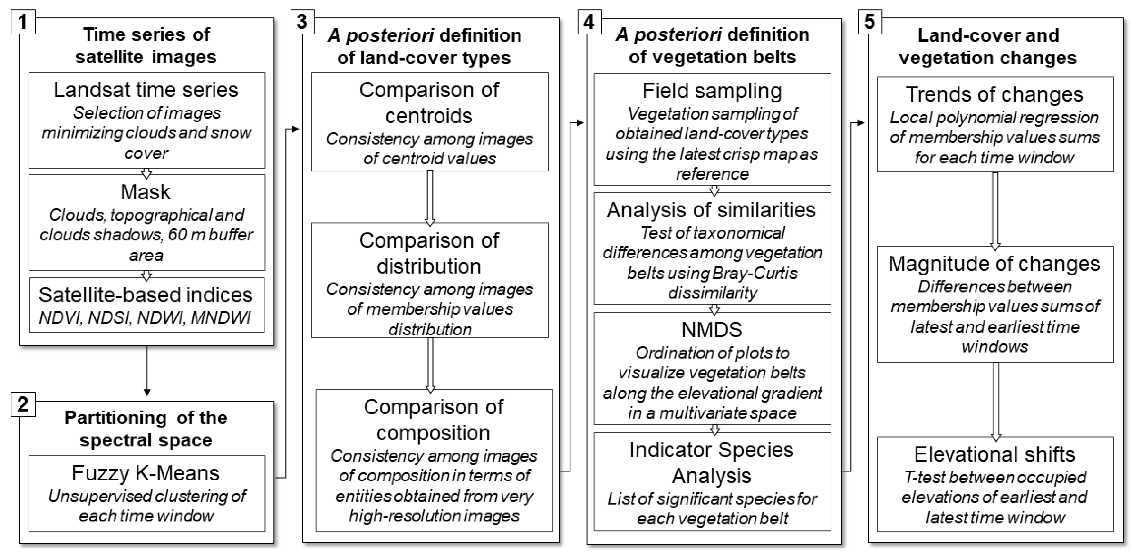
2. Materials and Methods
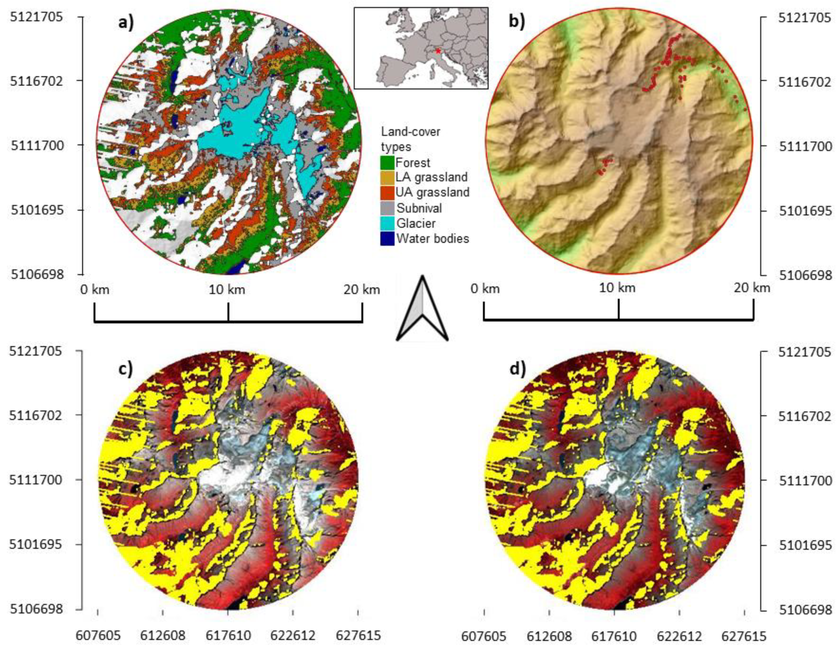
2.1. Study Area

We delimited the study area using a circular plot of 10 km radius (31,400 ha) centered in the largest Italian glacier in the Adamello-Brenta National Park (46°1487653016 N 10°5230462715 E; Figure 1). It occupies an elevational range of about 2370 m (from 1184 m to 3554 m a.s.l.) covered by subalpine forests, sub-alpine and alpine grasslands, subnival plant communities, glacier forelands, and the glacier itself. The mean annual temperature varies from 5 to −3 °C and precipitation varies from 800 to 1500 mm per year [22].

2.2. Collection and Manipulation of Satellite Images

We collected eleven available late-summer Landsat TM/ETM images (30 m × 30 m of resolution) spanning from 1987 to 2016 minimizing cloud and snow cover within the study area (Table 1). However, the high-mountain landscape of the study area is affected by frequent summer cloudiness, preventing the selection of more images for the central part of the summer period. Yet, the temporal distribution of selected satellite images was almost regular over the last 30 years, where on average, two years of gap occurred between two images (Table 1).
The collected images were aggregated in a time series. Given the high morphological heterogeneity of the studied landscape, topographical shadows were calculated using solar elevation and a digital elevation model at 25 m resolution using the doshade function of the ‘insol’ R package [23]. The occurrence of clouds and their shadows were detected using the F-mask function (probability threshold = 0.25) in QGIS software. Areas occupied by the topographic shadows and clouds and their shadows were combined with unreliable pixels due to defective functioning of the Landsat 7 sensor. Accordingly, the obtained mask was completed adding a buffer area of 60 m that was filtered out from selected images, which meant 32.7% of the study area. To reduce redundancy given by correlation of spectral bands, we transformed digital numbers of the obtained images to normalized indices which amplified characteristic signals of the different entities occurring in the study area. Accordingly, the use of digital numbers instead of surface reflectance did not affect the calculation of normalized indices. In detail, to account for vegetated pixels, we used the (1) Normalized Difference Vegetation Index (NDVI), to account for unvegetated pixels, we used the (2) Normalized Difference Soil Index (NDSI), and to account for ice and water, we used both the (3) Normalized Difference Water Index (NDWI) and the (4) Modified NDWI (MNDWI).

2.3. Time Series of Land-Cover Types

We adopted a post-classification comparison of the time series of satellite images which enabled us to evaluate changes in the occupied surfaces by land-cover types. The lack of historical field data in the study area prevented the use of supervised clustering approaches in which ground truth data can be used to train and validate a priori selected classes over space and time. Accordingly, we performed an unsupervised clustering approach to partition the spectral space into comparable and homogeneous classes over time. The clustering was followed by a posteriori evaluation of the temporal and spatial coherence of obtained classes and their definition in terms of spectral and entity composition. In detail, we grouped pixels into classes using a fuzzy k-means clustering performed on their normalized indices composition using the FKM function of the ‘fclust’ R package using 2 as the parameter of fuzziness [24]. This unsupervised technique of clustering assigned a membership degree (from 0 to 1) to each pixel for each class according to the similarity between the centroid of the group and the target pixel composition. The sum of membership values for each pixel corresponded to 1. Additionally, we converted fuzzy membership values to Boolean values using the highest values to obtain a corresponding hard classification of land-cover types (Figure 1a). We clustered separately each image, that represented a specific time window on the study area. After an evaluation of several combinations of classes’ numbers (i.e., 3, 6, and 7), 6 classes were then selected as the most exhaustive representation of the studied landscape without neglecting coherence among classes’ compositions from different time windows. Indeed, differently from the other classes’ combinations, the obtained 6 classes were coherent in each time window in terms of (i) centroid values defined by the four normalized indices values, (ii) geographic distribution of membership values, and (iii) entities’ coverages (Figures S1–S8). The latter evaluation consisted of defining hard classes using occupied elevations and composition in terms of main entities (i.e., trees, shrubs, herbs, unvegetated ground, and water and ice) obtained from very high-resolution images (VHR images) of the study area. For a more complete evaluation of classes’ composition, we included also a class composed of those pixels with membership values below 0.5 for all classes and, thus, resulted in a weaker assignment. In detail, we used two VHR images provided by Google Earth (i.e., 2007 and 2011 resulted to be visually interpretable) with the assumption that two was the minimum number of time windows needed to assess the temporal coherence of classes. Accordingly, we assessed a random sampling design stratified on membership values on the obtained fuzzy maps with a total of 1800 samples for each VHR image. We visually assessed percentage covers of the main entities for each sample, i.e., a 30 m × 30 m Landsat pixel. Details on the stratification of sampling design are provided in Figure S1. Eventually, the obtained land-cover types resulted in (1) herbaceous, shrub, and tree coverage in descending order of mean cover, and unvegetated ground, (2) high cover of herbaceous species and a low cover of unvegetated ground, (3) high cover of unvegetated ground and a low cover of herbaceous species, (4) unvegetated ground, (5) ice, and (6) water and ice. Among all, the sixth class was the weakest defined in terms of entities’ composition. The occurrence of temporary water pools (melting ice during summer, floods, and streams) due to the local daily weather made the delimitation of that land-cover type ambiguous in both high and medium resolution satellite images.

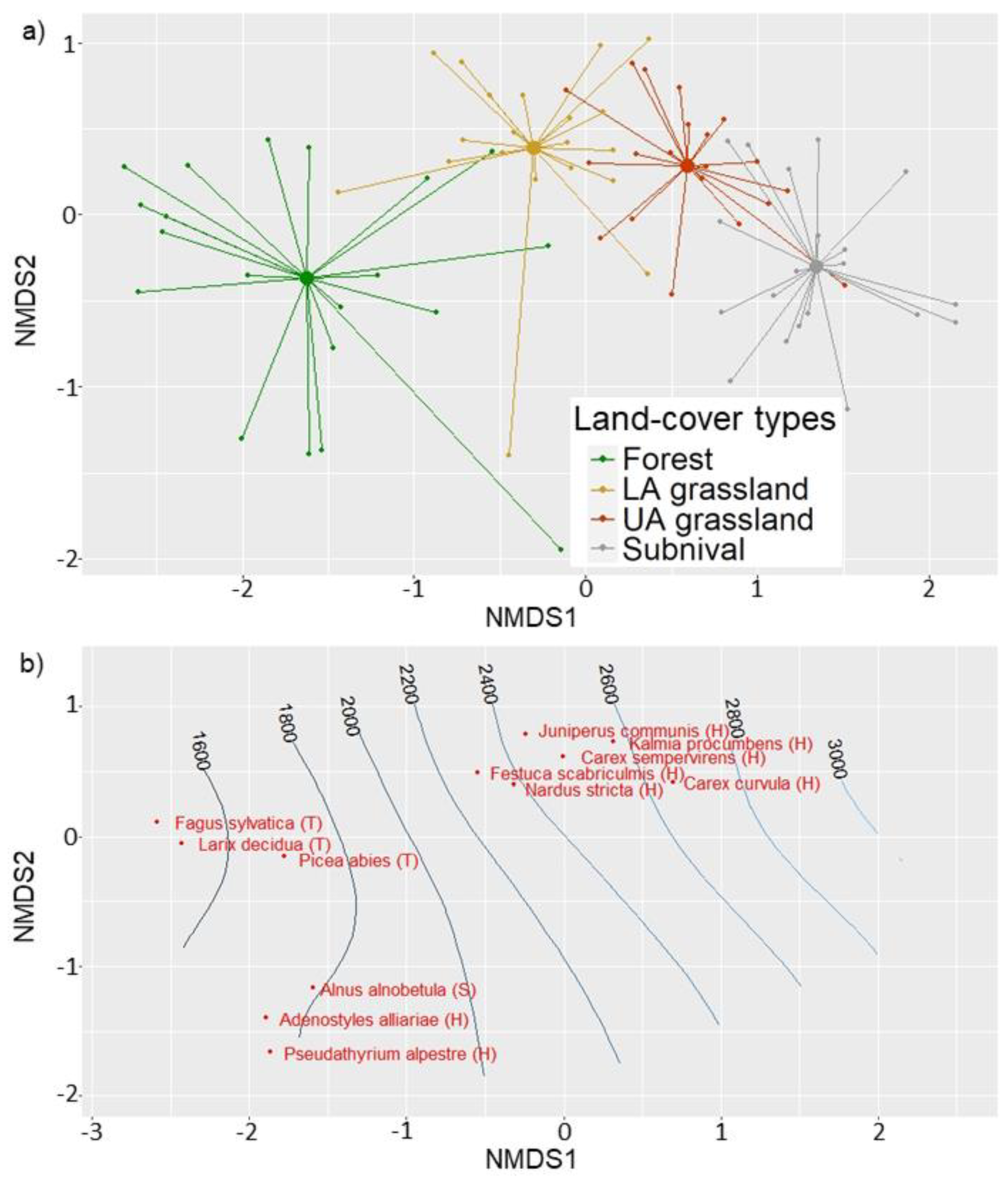
2.4. Definition of Vegetation Belts

The obtained land-cover types were assigned to vegetation belts based on their plant species composition. Therefore, a field sampling on plant communities was performed in 2018 and 2019 for all the land-cover types, except for 5 and 6. Due to the impervious landscape in the study area, complete randomization of the sampling design was not possible. We thus adopted a random sampling design assessed in the field following an altitudinal gradient in more accessible pathways. For each of the four land-cover types, 20 vegetation plots were assessed using the latest crisp map as a reference. The plot size was fixed according to the sampled plant community [25], ranging from 1 m2 for sparse alpine grasslands to 100 m2 for the forest stands. The taxonomy of species followed the most recent national checklist [26]. In each plot, a percentage cover of occurring species was visually estimated for each community layer which included the tree (growth height > 5 m), shrub (1 m < height > 5 m), and herb layer (height < 1 m). In total, a matrix composed of the percentage cover of 80 vegetation plots per 226 taxonomical entities was obtained. In order to test for differences in the taxonomical composition of classes, an analysis of similarities was performed using the Bray-Curtis dissimilarity (statistic R = 0.5599; p-value = 0.001). The Bray-Curtis dissimilarity metric results are suitable for community data, ignoring double zeros and having an upper limit of 1, in contrast to most used metrics such as the Euclidean distance [27]. For this, we used the anosim function of the ‘vegan’ R package with 999 permutations [28].
In order to evaluate ecological patterns of communities and dominant species along the elevational gradient, Non-Metric Multidimensional Scaling (NMDS) based on natural logarithm data transformation and Bray-Curtis dissimilarity was used (final stress = 0.1137; Figure 2).
Accordingly, dominant species were identified as those species that reached a cover exceeding 35% for more than the 5% of samples within the class samples. Indicator species analyses were performed to obtain significant species, which occur mainly, or only, in the target class. Therefore, the multipatt function of the ‘indicspecies’ R package was used with 999 permutations [29]. Based on the species composition summarized in Table S1, the first land-cover type was associated with the subalpine forest vegetation, dominated mainly by Picea abies and Alnus alnobetula, and characterized by dwarf shrubs and herbs such as Milium effusum, Prenanthes purpurea, and Vaccinium myrtillus. The second land-cover type was associated with lower alpine grasslands (hereinafter LA grassland). The LA grassland is dominated mainly by Festuca scabriculmis and Nardus stricta and is characterized by species such as Juniperus communis and Carex sempervirens. The third land-cover type was associated with the upper alpine grasslands (hereinafter UA grassland) dominated by Carex curvula and Kalmia procumbens. The UA grassland is characterized by species such Salix herbacea and Agrostis rupestris. The fourth land-cover type was associated with the subnival vegetation which mainly occurred in small patches over rocky screes. Such a class is dominated by Carex curvula and characterized by species such as Ranunculus glacialis, Poa alpina, Saxifraga bryoides, Leucanthemopsis alpina, and Saxifraga bryoides. The remaining two land-cover types were defined as the water bodies and glaciers.

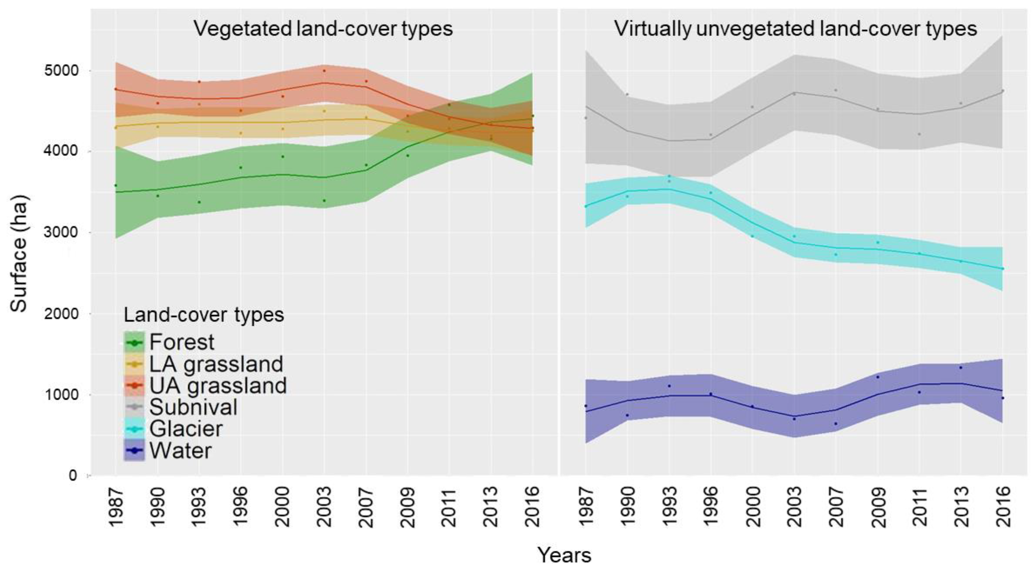
2.5. Trends and Magnitude of Land-Cover Changes

The surface occupied by a land-cover type in a specific time window was calculated summing membership values of the target type, which were assumed as an estimate of the occupied pixel portion [30,31,32]. This sum was then converted to hectares considering a surface of 900 m2 for each pixel. Trends in the occupied surface by land-cover types were obtained smoothing calculated values for all time windows with a local polynomial regression (loess function in R). The magnitude of change in the occupied surface for each land-cover type was obtained by subtracting surfaces of the earliest time window from the latest one. Accordingly, absolute (hectares) and relative (percentages) magnitudes of changes were calculated in relation to the earliest time window. To test for the elevational shift of types over time, a t-test was applied to elevations corresponding to target crisp pixels of the earliest and latest time windows. Elevation values were obtained from a digital elevation model of 25 m of resolution readapted to the 30 m × 30 m Landsat grid.
All the analyses were performed using R [33] and QGIS software [34]. The general workflow was graphically summarized in Figure 3 and provided in an R coding script (File S2). Results were illustrated using graphic functions of the ‘ggplot2′ package in R [35].

3. Results

Trends and magnitude of changes in the occupied surfaces by the defined land-cover types are shown in Figure 4 and Figure 5, respectively.
While the forest type showed a continuous positive trend in the surface which accelerated from 2009 on, LA grassland remained almost stable in their occurrence. The former increased in surface area by 24% (862 ha) from 1987, whereas the latter decreased by 0.9% which means 40 ha less. The UA grassland showed an opposite trend to the forest type, reaching a loss of 10% (−480 ha) in the occupied surface in 2016. The surface of the subnival vegetation belt fluctuated over time but overall increased by 8% which equals 336 ha. The glacier type showed a strong decrease in the occupied surface during the first half of the time series (1987–2003) which slowed down in the second half (2003–2016). The overall decrease of the glacier surface amounts to 23% which is 774 ha less. The class referencing water bodies showed a slight alternation of decreasing and increasing phases with a final increase of 11% (96 ha). We performed the t-test to verify an elevational shift from 1987 to 2016 for all the land-cover types, except the water type due to its poor reliability on distribution over time and space. All the tested types showed a significant shift in mean elevation (Figure 6). We observed the major upward shift in the subnival land-cover type (70 m) followed by forest (45 m), glacier (33 m), and LA grassland (24 m). The UA grassland showed instead a slight downward shift with −8 m.

4. Discussion

Regional and global studies demonstrated that ranges of plants occurring in mountain landscapes are shifting upwards due to global warming, although downward shifts can also occur [9,36,37,38]. However, species occupying lower elevations resulted in having a faster upward shift than species at higher elevations [37]. Despite the general agreement on the urgent need to monitor dynamic processes of alpine plants, there is a lack of studies proposing an approach to measure and evaluate vegetation upward shifts and ranges shrinking at the landscape level. The present study combines a thirty-years Landsat time series (i.e., 1987–2016) with knowledge gained from plant communities’ surveys to measure mountain vegetation responses in the era of climate change and the Anthropocene.
The comparison of land-cover types’ distribution over time highlighted rapid and profound changes ongoing in the surrounding of the Adamello glacier in N Italy over the last three decades. The surface occupied by forest has expanded upward as much as the glacier has retreated which means little less than a quarter of their initial occupied surface. Different surface tradeoffs and altitudinal shifts occurred between the previously mentioned lowest and highest elevational zones. While LA grassland has shifted at higher elevations maintaining stable its occupied surface, UA grassland showed a similar decrease in the occupied surfaces at both, its lower and higher edges, for a total loss of 10% of its original surface. On the other hand, the subnival vegetation belt has gained 8% of surface area from the glacial retreat with an upward shift of 70 m. In line with previous studies [9,36,37], the faster upward shift of species at lower elevations than those at higher elevations is reducing the surface area occupied by alpine vegetation. This divergent spatio-temporal distribution pattern of land-cover types and associated vegetation belts suggests a differential role of biotic and abiotic factors across the altitudinal zonation. Amongst them, we addressed large topographic differences within the zones of the elevational gradient.
The unsupervised approach applied here, allows us to map and identify mountain and alpine systems such as glaciers, water bodies, and different vegetation belts in terms of satellite-based signal and, where applicable, plant species composition of such vegetation belts. Indeed, the obtained land-cover types resulted to be coherent over time, thus, overcoming the lack of historical field data commonly used to train and validate (semi)supervised clustering approaches. The adopted fuzzy approach provided values of the occupied surfaces considering both the continuous distribution of systems as well as the uncertainty of pixel classification [39]. However, empirical studies are needed to evaluate the accuracy of the delimitation of fuzzy surfaces [30,31,32]. Accordingly, training and validation ground truth data should be used in a (semi)supervised approach where fuzzy matrices are implemented for the accuracy assessment of land-cover mapping [21]. Our results show that the Landsat resolution can better identify forest stands than subnival community patches. Indeed, the low values of plant coverage characterizing this latter vegetation belt prevented an accurate delimitation of poorly vegetated pixels at a medium resolution of Landsat images. Given this evidence, the obtained surfaces of the subnival vegetation belt should be considered as the potential area of occupancy, which comprises both occupied and suitable but not occupied areas. Additionally, the water bodies were poorly delimited by our approach. Since water occurrence in such an environment strongly depends on local weather, its identification was limited by the low spatio-temporal resolution of the time series. A further improvement of the presented approach should be to consider intra-annual variation of the satellite signal using high-frequency images, such as those from the Sentinel-2 program, enabling the derivation of satellite-based phenological metrics [17,40]. An advantage of the fuzzy approach is the easy conversion towards a crisp classification of pixels which enabled robust descriptions of group cores in terms of entities and species co-occurrences. Once the above-mentioned exceptions of the approach are considered, the overall estimation of main system changes in the occupied surfaces can be considered as reliable for estimating past landscape changes.
The most rapid and strong changes that occurred in the study area refer to the glacier retreat and forest expansion, which are mainly driven by climate and land-use changes, respectively [39,41]. The rapid decrease registered during the 1980s and 1990s in the occupied surface by the Adamello glacier is in line with the results of local as well as regional studies [41,42,43,44,45]. However, during the second period of the time series (2003 to 2016), we found a slower glacier retreat in terms of surface area. This disparity in the retreat velocity can be due to an initial rapid decrease in the occupied surfaces by valley glaciers (e.g., Mandrone or Salarno), which are characterized by a lower thickness than the plateau area (Pian di Neve, ~270 m of depth [43,46,47]). This drastic reduction in the extension of the Adamello glacier has most likely been followed by a reduction in the thickness of the plateau and valley glaciers, which is, however, undetectable by satellite images. At the same time, the latter process could have been slowed down by the thermal inertia of the glacier mass [48]. On the lower elevations of the studied area, the reported expansion of the forest type should be considered as the result of stands’ development and maturation driven by land abandonment, which occurred during the last century [12,41]. The recorded upward shift in the mean occupied elevation by this vegetation belt may be due to the shrub encroachment colonizing from steep to moderate rocky slopes and screes because of the decreased grazing pressure. This has been reported in the Alps for Alnus alnobetula [49], a forest indicator species in our study.
Between these two opposite trends shown by the glacier and forest types, a more complex dynamic resulted from the temporal distribution of the three land-cover types characterized by herbs, grasses, and unvegetated soil. The moderate upward shift of the occupied surface by the LA grasslands corresponded to a virtually absent elevational shift and a reduction of the surface occupied by the UA grasslands. The upward expansion of warm-adapted alpine species occupying lower elevations to the detriment of the cold-adapted alpine species occupying higher elevations has been explained as an effect of global warming which is also called the thermophilization phenomena [7,50]. On the other hand, UA grasslands dominated by Carex curvula showed no ability to follow this general upward shift of alpine vegetation. Several studies observed a similar time lag in the upward shift of species occurring at the transitional zone between the alpine and subnival zones, such as Carex curvula and Poa alpina [51,52,53,54,55,56,57]. The declining trend of UA grasslands contrasts with the increasing availability of ice-free sites of the subnival land-cover type. This could depend on the instability of new ice-free sites due to the permafrost degradation which increases the number of unsafe sites to colonize [5,50,52]. Recent studies based on field resurveys reported a decline of subnival species at their lower border mainly driven by global warming [5,48]. The decreasing availability of safe sites and dispersal limitations of subnival species due to environmental changes can lead to a threat and decline of this vegetation belt [5,58]. In the context of increasing temperature, the different observed spatio-temporal trends in the occupied surfaces suggest a decline of the available surface at the transitional zones of alpine and subnival belts. This trend may rise both the extinction debt and colonization credits of high-mountain species, which are the results of a delay in the colonization or extinction processes following environmental changes [48,59]. Such scenarios depend on the temporal and spatial magnitude of the lack of available surface of respective vegetation belts [7,58].

5. Conclusions

The combination of field vegetation and remotely-sensed data enabled a consistent evaluation of land-cover changes and vegetation responses in an Alpine landscape to the last 30 years of environmental changes. Despite the poor time series in terms of time windows due to the low temporal frequency of the used satellite products and mountain cloudiness, our findings resulted in line with studies based on field observations. We indeed observed a general upward shift of mid-elevation vegetation with a consequent reduction of surfaces occupied by high-elevation vegetation. We suggest that medium- to high-resolution remotely sensed data should be used in combination with ecological data to analyze vegetation over wide spatio-temporal scales and different biological levels. Moreover, the future collection of high-frequency images, such as Sentinel-2 products, will enable a more effective mapping of land-cover types throughout the use of satellite-based phenological indices. These reliable techniques and data will enable an accurate monitoring system of land-cover and vegetation dynamics detecting their expansion, retreat, or shift in the context of current global change and enabling an accurate evaluation of the magnitude of changes. The standardized observations freely accessible from satellite programs could be used to track critical sites in natural reserves over time and space reducing the workload on the field, and in turn, to optimize practices for the conservation of biodiversity at a large scale. Because climate change is expected to threaten the mountain vegetation across the whole globe, monitoring networks using standardized protocols are important to assess such changes to a large geographical extent. Although a rigorous protocol cannot be deduced from our study, our approach can be intended as a starting point to identify vegetation change that can be applied in different mountain and glacier systems worldwide for a much larger comparison.

Supplementary Materials

The following are available online at https://0-www-mdpi-com.brum.beds.ac.uk/2072-4292/13/1/134/s1, File S1: Methods and results for the evaluation of fuzzy clustering applied to the thirty-years time-time series composed by eleven Landsat images. Table S1: List of dominant and indicator species of sampled vegetation belts. File S2: R code summarizing the workflow adopted in this study using an example of time series composed by two images.

Author Contributions

Conceptualization, N.A., C.W., K.O. and S.Z.; methodology, N.A., D.R. and G.M.; field survey, N.A. and G.M. formal analysis, N.A. and G.M.; writing—original draft preparation, N.A.; writing—review and editing, N.A., C.W., D.R., G.M., K.O. and S.Z. All authors have read and agreed to the published version of the manuscript.

Funding

This work is a contribution to the project CALICE-Calibrating biodiversity in glacier ice, a multidisciplinary program between the University of Innsbruck, the Free University of Bozen—Bolzano and the Fondazione Edmund Mach in San Michele. This is the CALICE project publication no. 3. This work was supported by the Open Access Publishing Fund of the Free University of Bozen-Bolzano.

Institutional Review Board Statement

Not applicable.

Informed Consent Statement

Not applicable.

Data Availability Statement

Vegetation plots collected in this study have been archived in the national database “Vegetation Plots Database–La Sapienza” accessible from the “European Vegetation Archive”.

Acknowledgments

We would like to thank the personnel of Adamello Brenta national reserve who enabled the vegetation surveys. We also thank Rita Tonin and Daniela Festi for the valuable support during the vegetation sampling.

Conflicts of Interest

The authors declare no conflict of interest.

References

  1. Körner, C. Why are there global gradients in species richness? Mountains might hold the answer. Trends Ecol. Evol. 2000, 15, 513–514. [Google Scholar] [CrossRef]
  2. Jump, A.S.; Mátyás, C.; Peñuelas, J. The altitude-for-latitude disparity in the range retractions of woody species. Trends Ecol. Evol. 2009, 24, 694–701. [Google Scholar] [CrossRef] [PubMed] [Green Version]
  3. von Humboldt, A.; Bonpland, A. Ideen zu Einer Geographic der Pflanzen Nebst Einem Naturgemälde der Tropenländer; Tübingen: Paris, France, 1807. [Google Scholar]
  4. Erschbamer, B.; Caccianiga, M.S. Glacier Forelands: Lessons of Plant Population and Community Development. Prog. Bot. 2016, 78, 259–284. [Google Scholar] [CrossRef]
  5. Erschbamer, B.; Niederfriniger Schlag, R.; Winkler, E. Colonization processes on a central alpine glacier foreland. J. Veg. Sci. 2008, 19, 855–862. [Google Scholar] [CrossRef]
  6. Wellstein, C.; Uehlinger, U.; Zah, R. Terrestrial Floodplain Vegetation. In Ecology of a Glacial Flood Plain; Ward, J.V., Uehlinger, U., Eds.; Springer: Dordrecht, The Netherlands, 2003; pp. 109–121. [Google Scholar]
  7. Steinbauer, M.J.; Grytnes, J.A.; Jurasinski, G.; Kulonen, A.; Lenoir, J.; Pauli, H.; Rixen, C.; Winkler, M.; Bardy-Durchhalter, M.; Barni, E.; et al. Accelerated increase in plant species richness on mountain summits is linked to warming. Nature 2018, 556, 231–234. [Google Scholar] [CrossRef]
  8. Buitenwerf, R.; Sandel, B.; Normand, S.; Mimet, A.; Svenning, J.C. Land surface greening suggests vigorous woody regrowth throughout European semi-natural vegetation. Glob. Chang. Biol. 2018, 24, 5789–5801. [Google Scholar] [CrossRef] [Green Version]
  9. Lenoir, J.; Gégout, J.C.; Marquet, P.A.; De Ruffray, P.; Brisse, H. A significant upward shift in plant species optimum elevation during the 20th century. Science 2008, 320, 1768–1771. [Google Scholar] [CrossRef]
  10. Grabherr, G.; Gottfried, M.; Pauli, H. Climate effects on mountain plants. Nature 1994, 369, 448. [Google Scholar] [CrossRef]
  11. Tasser, E.; Leitinger, G.; Tappeiner, U. Climate change versus land-use change—What affects the mountain landscapes more? Land Use Policy 2017, 60, 60–72. [Google Scholar] [CrossRef]
  12. Bodin, J.; Badeau, V.; Bruno, E.; Cluzeau, C.; Moisselin, J.M.; Walther, G.R.; Dupouey, J.L. Shifts of forest species along an elevational gradient in Southeast France: Climate change or stand maturation? J. Veg. Sci. 2013, 24, 269–283. [Google Scholar] [CrossRef]
  13. COM. Communication from the commission to the European parliament, the council, the European economic and social committee and the committee of the regions. In EU Biodiversity Strategy for 2030—Bringing Nature Back into Our Lives; No. 380 Final; European Commission: Brussels, Belgium, 2020. [Google Scholar]
  14. Gillespie, T.W.; Foody, G.M.; Rocchini, D.; Giorgi, A.P.; Saatchi, S. Measuring and modelling biodiversity from space. Prog. Phys. Geogr. 2008, 32, 203–221. [Google Scholar] [CrossRef]
  15. Pereira, H.M.; Ferrier, S.; Walters, M.; Geller, G.N.; Jongman, R.H.G.; Scholes, R.J.; Bruford, M.W.; Brummitt, N.; Butchart, S.H.M.; Cardoso, A.C.; et al. Essential Biodiversity Variables. Science 2013, 339, 277–278. [Google Scholar] [CrossRef] [PubMed] [Green Version]
  16. Rocchini, D.; Balkenhol, N.; Carter, G.A.; Foody, G.M.; Gillespie, T.W.; He, K.S.; Kark, S.; Levin, N.; Lucas, K.; Luoto, M.; et al. Remotely sensed spectral heterogeneity as a proxy of species diversity: Recent advances and open challenges. Ecol. Inform. 2010, 5, 318–329. [Google Scholar] [CrossRef]
  17. Pesaresi, S.; Mancini, A.; Quattrini, G.; Casavecchia, S. Mapping mediterranean forest plant associations and habitats with functional principal component analysis using Landsat 8 NDVI time series. Remote Sens. 2020, 12, 1132. [Google Scholar] [CrossRef] [Green Version]
  18. Marzialetti, F.; Giulio, S.; Malavasi, M.; Sperandii, M.G.; Acosta, A.T.R.; Carranza, M.L. Capturing coastal dune natural vegetation types using a phenology-based mapping approach: The potential of Sentinel-2. Remote Sens. 2019, 11, 1506. [Google Scholar] [CrossRef] [Green Version]
  19. Wegmann, M.; Leutner, B.; Dech, S. Remote Sensing and GIS for Ecologists: Using Open Source Software; Pelagic Publishing Ltd.: Exeter, UK, 2016. [Google Scholar]
  20. Rocchini, D. While Boolean sets non-gently rip: A theoretical framework on fuzzy sets for mapping landscape patterns. Ecol. Complex. 2010, 7, 125–129. [Google Scholar] [CrossRef]
  21. Rocchini, D.; Foody, G.M.; Nagendra, H.; Ricotta, C.; Anand, M.; He, K.S.; Amici, V.; Kleinschmit, B.; Förster, M.; Schmidtlein, S.; et al. Uncertainty in ecosystem mapping by remote sensing. Comput. Geosci. 2013, 50, 128–135. [Google Scholar] [CrossRef]
  22. Gentili, R.; Armiraglio, S.; Sgorbati, S.; Baroni, C. Geomorphological disturbance affects ecological driving forces and plant turnover along an altitudinal stress gradient on alpine slopes. Plant Ecol. 2013, 214, 571–586. [Google Scholar] [CrossRef]
  23. Corripio, J.G. Insol: Solar Radiation. R Package Version 1.2.1. 2019. Available online: https://cran.r-project.org/package=insol (accessed on 24 August 2018).
  24. Ferraro, M.B.; Giordani, P.; Serafini, A. fclust: An R Package for Fuzzy Clustering. R J. 2019, 11, 198. Available online: https://journal.r-project.org/archive/2019/RJ-2019-017/RJ-2019-017.pdf (accessed on 15 November 2018). [CrossRef]
  25. Chytrý, M.; Otýpková, Z. Plot sizes used for phytosociological sampling of European vegetation. J. Veg. Sci. 2003, 14, 563–570. [Google Scholar] [CrossRef]
  26. Bartolucci, F.; Peruzzi, L.; Galasso, G.; Albano, A.; Alessandrini, A.; Ardenghi, N.M.G.; Astuti, G.; Bacchetta, G.; Ballelli, S.; Banfi, E.; et al. An updated checklist of the vascular flora native to Italy. Plant Biosyst. 2018, 152, 179–303. [Google Scholar] [CrossRef]
  27. Bray, J.R.; Curtis, J.T. An ordination of the upland forest communities of southern Wisconsin. Ecol. Monogr. 1957, 27, 325–349. [Google Scholar] [CrossRef]
  28. Oksanen, J.; Blanchet, F.G.; Friendly, M.; Kindt, R.; Legendre, P.; McGlinn, D.; Minchin, P.R.; O’Hara, R.B.; Simpson, G.L.; Solymos, P.; et al. Vegan: Community Ecology Package. R Package Version 2.5-6. 2019. Available online: https://CRAN.R-project.org/package=vegan (accessed on 21 January 2019).
  29. De Caceres, M.; Legendre, P. Associations between species and groups of sites: Indices and statistical inference. Ecology 2009, 90, 3566–3574. [Google Scholar] [CrossRef] [PubMed]
  30. Cheng, T. Fuzzy objects: Their changes and uncertainties. Photogramm. Eng. Remote Sens. 2002, 68, 41–49. [Google Scholar]
  31. Fisher, P.; Arnot, C.; Wadsworth, R.; Wellens, J. Detecting change in vague interpretations of landscapes. Ecol. Inform. 2006, 1, 163–178. [Google Scholar] [CrossRef]
  32. Blanco, P.D.; Colditz, R.R.; López Saldaña, G.; Hardtke, L.A.; Llamas, R.M.; Mari, N.A.; Fischer, A.; Caride, C.; Aceñolaza, P.G.; del Valle, H.F.; et al. A land cover map of Latin America and the Caribbean in the framework of the SERENA project. Remote Sens. Environ. 2013, 132, 13–31. [Google Scholar] [CrossRef]
  33. R Team Core. R: A Language and Environment for Statistical Computing; R Foundation for Statistical Computing: Vienna, Austria, 2020. [Google Scholar]
  34. QGIS.org QGIS Geographic Information System. QGIS Association. Available online: http://www.qgis.org (accessed on 29 June 2018).
  35. Wickham, H. ggplot2: Elegant Graphics for Data Analysis; Springer: New York, NY, USA, 2016; Available online: https://ggplot2.tidyverse.org (accessed on 24 June 2018).
  36. Freeman, B.G.; Lee-Yaw, J.A.; Sunday, J.M.; Hargreaves, A.L. Expanding, shifting and shrinking: The impact of global warming on species’ elevational distributions. Glob. Ecol. Biogeogr. 2018, 27, 1268–1276. [Google Scholar] [CrossRef]
  37. Rumpf, S.B.; Hülber, K.; Klonner, G.; Moser, D.; Schütz, M.; Wessely, J.; Willner, W.; Zimmermann, N.E.; Dullinger, S. Range dynamics of mountain plants decrease with elevation. Proc. Natl. Acad. Sci. USA 2018, 115, 1848–1853. [Google Scholar] [CrossRef] [Green Version]
  38. Lenoir, J.; Gégout, J.C.; Guisan, A.; Vittoz, P.; Wohlgemuth, T.; Zimmermann, N.E.; Dullinger, S.; Pauli, H.; Willner, W.; Svenning, J.C. Going against the flow: Potential mechanisms for unexpected downslope range shifts in a warming climate. Ecography 2010, 33, 295–303. [Google Scholar] [CrossRef]
  39. Rocchini, D.; Hortal, J.; Lengyel, S.; Lobo, J.M.; Jiménez-Valverde, A.; Ricotta, C.; Bacaro, G.; Chiarucci, A. Accounting for uncertainty when mapping species distributions: The need for maps of ignorance. Prog. Phys. Geogr. 2011, 35, 211–226. [Google Scholar] [CrossRef]
  40. Wakulinśka, M.; Marcinkowska-Ochtyra, A. Multi-temporal sentinel-2 data in classification of mountain vegetation. Remote Sens. 2020, 12, 2696. [Google Scholar] [CrossRef]
  41. Tasser, E.; Walde, J.; Tappeiner, U.; Teutsch, A.; Noggler, W. Land use changes and natural reforestation in the Eastern Central Alps. Agric. Ecosyst. Environ. 2007, 118, 115–129. [Google Scholar] [CrossRef]
  42. Diolaiuti, G.; Bocchiola, D.; D’agata, C.; Smiraglia, C. Evidence of climate change impact upon glaciers’ recession within the Italian Alps: The case of Lombardy glaciers. Theor. Appl. Climatol. 2012, 109, 429–445. [Google Scholar] [CrossRef]
  43. Festi, D.; Schwikowski, M.; Maggi, V.; Oeggl, K.; Jenk, T.M. Significant mass loss in the accumulation area of the Adamello glacier indicated by the chronology of a 46 m ice core. Cryosphere Discuss. 2020, 1–13. [Google Scholar] [CrossRef]
  44. Gardent, M.; Rabatel, A.; Dedieu, J.P.; Deline, P. Multitemporal glacier inventory of the French Alps from the late 1960s to the late 2000s. Glob. Planet. Chang. 2014, 120, 24–37. [Google Scholar] [CrossRef]
  45. Maragno, D.; Diolaiuti, G.; D’Agata, C.; Mihalcea, C.; Bocchiola, D.; Janetti, E.B.; Riccardi, A.; Smiraglia, C. New evidence from Italy (Adamello Group, Lombardy) for analysing the ongoing decline of Alpine glaciers. Geogr. Fis. Din. Quat. 2009, 32, 31–39. [Google Scholar]
  46. Festi, D. Now or never: The study of disappearing ice archives in the time of global warming. Alp. Mediterr. Quat. 2018, 31, 73–78. [Google Scholar]
  47. Picotti, S.; Francese, R.; Giorgi, M.; Pettenati, F.; Carcione, J.M. Estimation of glacier thicknesses and basal properties using the horizontal-to-vertical component spectral ratio (HVSR) technique from passive seismic data. J. Glaciol. 2017, 63, 229–248. [Google Scholar] [CrossRef] [Green Version]
  48. Lamprecht, A.; Semenchuk, P.R.; Steinbauer, K.; Winkler, M.; Pauli, H. Climate change leads to accelerated transformation of high-elevation vegetation in the central Alps. New Phytol. 2018, 220, 447–459. [Google Scholar] [CrossRef]
  49. Caviezel, C.; Hunziker, M.; Khun, N.J. Green alder encroachment in the European Alps: The need for analyzing the spread of a native-invasive species across spatial data. Catena 2017, 159, 149–158. [Google Scholar] [CrossRef]
  50. Gottfried, M.; Pauli, H.; Futschik, A.; Akhalkatsi, M.; Barančok, P.; Benito Alonso, J.L.; Coldea, G.; Dick, J.; Erschbamer, B.; Fernández Calzado, M.R.; et al. Continent-wide response of mountain vegetation to climate change. Nat. Clim. Chang. 2012, 2, 111–115. [Google Scholar] [CrossRef]
  51. Steinbauer, K.; Lamprecht, A.; Semenchuk, P.; Winkler, M.; Pauli, H. Dieback and expansions: Species-specific responses during 20 years of amplified warming in the high Alps. Alp. Bot. 2020, 130, 1–11. [Google Scholar] [CrossRef] [Green Version]
  52. Parolo, G.; Rossi, G. Upward migration of vascular plants following a climate warming trend in the Alps. Basic Appl. Ecol. 2008, 9, 100–107. [Google Scholar] [CrossRef]
  53. Pauli, H.; Gottfried, M.; Reiter, K.; Klettner, C.; Grabherr, G. Signals of range expansions and contractions of vascular plants in the high Alps: Observations (1994-2004) at the GLORIA *master site Schrankogel, Tyrol, Austria. Glob. Chang. Biol. 2007, 13, 147–156. [Google Scholar] [CrossRef]
  54. Cannone, N.; Pignatti, S. Ecological responses of plant species and communities to climate warming: Upward shift or range filling processes? Clim. Chang. 2014, 123, 201–214. [Google Scholar] [CrossRef]
  55. Cannone, N.; Sgorbati, S.; Guglielmin, M. Unexpected impacts of climate change on alpine vegetation. Front. Ecol. Environ. 2007, 5, 360–364. [Google Scholar] [CrossRef] [Green Version]
  56. Pauli, H.; Gottfried, M.; Grabherr, G. Effects of climate change on the alpine and nival vegetation of the Alps. J. Mt. Ecol. 2003, 7, 9–12. [Google Scholar]
  57. Rosbakh, S.; Bernhardt-Römermann, M.; Poschlod, P. Elevation matters: Contrasting effects of climate change on the vegetation development at different elevations in the Bavarian Alps. Alp. Bot. 2014, 124, 143–154. [Google Scholar] [CrossRef]
  58. Tonin, R.; Gerdol, R.; Tomaselli, M.; Petraglia, A.; Carbognani, M.; Wellstein, C. Intraspecific functional trait response to advanced snowmelt suggests increase of growth potential but decrease of seed production in snowbed plant species. Front. Plant Sci. 2019, 10, 289. [Google Scholar] [CrossRef]
  59. Rumpf, S.B.; Hülber, K.; Wessely, J.; Willner, W.; Moser, D.; Gattringer, A.; Klonner, G.; Zimmermann, N.E.; Dullinger, S. Extinction debts and colonization credits of non-forest plants in the European Alps. Nat. Commun. 2019, 10, 4293. [Google Scholar] [CrossRef] [Green Version]
Figure 1. Location of the study area. The circular area of 10 km radius centered in the Adamello glacier (Geographic coordinate system WGS84: 10.52 E, 46.15 N) is shown with (a) the distribution of land-cover types derived from the hard classification of the latest Landsat image (2016); (b) reliefs highlighted by a green-brown color gradient with vegetation plots represented by red dots; the (c) earliest (1987) and (d) latest (2016) images of the time series are shown using false-colors images (green, red, near-infrared bands). Unreliable pixels not considered in the analyses due to shadows and snow occurrences are highlighted in yellow.
Remotesensing 13 00134 g001
Figure 2. The Non-Metric Multidimensional Scaling (NMDS) bi-plots of the 80 vegetation plots sampled for the four vegetation belts. (a) A spider plot of the samples grouped according land-cover types and (b) a bi-plot with the main occurrence of dominant species and the corresponding elevation gradient are shown. Dominant species were defined as those with a cover higher than 35% for more than the 5% of samples within vegetation type. Species layers are shown in brackets–i.e., T for tree, S for shrub, and H for herb layers.
Remotesensing 13 00134 g002
Figure 3. The general workflow graphically summarized in five steps. It consists of a post-classification comparison of land-cover types and vegetation belts over a time series using a posteriori definition of classes.
Remotesensing 13 00134 g003
Figure 4. Trends in the occupied surfaces (ha) by the six land-cover types over thirty years (1987–2016) obtained using local polynomial regression. Vegetated and virtually unvegetated areas are shown in the two panels separately. Surfaces were obtained summing membership values of fuzzy clusters for each time window. The shaded colored areas refer to 95% confidence intervals.
Remotesensing 13 00134 g004
Figure 5. Magnitude of changes in the occupied surfaces estimated for the six land-cover types over the last thirty years. The (a) absolute (hectares) and (b) relative (percentage) magnitude values were estimated subtracting sums of fuzzy membership values in 1987 from those of the 2016 time window. Magnitude values for each type are delimited by a white line, whereas increasing and decreasing values are delimited by the vertical black line.
Remotesensing 13 00134 g005
Figure 6. Elevational distribution of land-cover types over time derived by Landsat images and corresponding indicator species for the four vegetation belts derived by field sampling. (a) Significant elevational shifts of the occupied surfaces by land-cover types that occurred between 1987 and 2016. Curves were smoothed using 115 elevational breaks of 20 m. (b) Density plots of the most significant indicator species (p-values < 0.001) along the elevational gradient. Species are grouped in vegetation belts following land-cover types. Species layers are provided between brackets (T for tree, S for shrub, and H for herb layers).
Remotesensing 13 00134 g006
Table 1. List of the eleven Landsat images composing the thirty-years time series. Details about images are provided in the table.
Nr.Acquisition DateMissionSensorIdentifierScene Cloud Cover
120 September 1987Landsat 5TMLT51930281987263XXX026%
212 September 1990Landsat 5TMLT51930281990255FUI005%
320 September 1993Landsat 5TMLT51930281993263FUI003%
426 July 1996Landsat 5TMLT51930281996208FUI003%
522 August 2000Landsat 5TMLT51930282000235FUI0010%
616 September 2003Landsat 5TMLT51930282003259MTI012%
711 September 2007Landsat 5TMLT51930282007254MOR0013%
88 September 2009Landsat 7ETMLE71930282009251ASN001%
921 August 2011Landsat 5TMLT51930282011233MOR001%
103 September 2013Landsat 7ETMLE71930282013246ASN001%
1126 August 2016Landsat 7ETMLE71930282016239NSG0015%
Publisher’s Note: MDPI stays neutral with regard to jurisdictional claims in published maps and institutional affiliations.

