Detecting Tree Species Effects on Forest Canopy Temperatures with Thermal Remote Sensing: The Role of Spatial Resolution

Abstract

Canopy temperatures are important for understanding tree physiology, ecology, and their cooling potential, which provides a valuable ecosystem service, especially in urban environments. Linkages between tree species composition in forest stands and air temperatures remain challenging to quantify, as the establishment and maintenance of onsite sensor networks is time-consuming and costly. Remotely-sensed land surface temperature (LST) observations can potentially acquire spatially distributed crown temperature data more efficiently. We analyzed how tree species modify canopy air temperature at an urban floodplain forest (Leipzig, Germany) site equipped with a detailed onsite sensor network, and explored whether mono-temporal thermal remote sensing observations (August, 2016) at different spatial scales could be used to model air temperatures at the tree crown level. Based on the sensor-network data, we found interspecific differences in summer air temperature to vary temporally and spatially, with mean differences between coldest and warmest tree species of 1 °C, and reaching maxima of up to 4 °C for the upper and lower canopy region. The detectability of species-specific differences in canopy surface temperature was found to be similarly feasible when comparing high-resolution airborne LST data to the airborne LST data aggregated to 30 m pixel size. To realize a spatial resolution of 30 m with regularly acquired data, we found the downscaling of Landsat 8 thermal data to be a valid alternative to airborne data, although detected between-species differences in surface temperature were less expressed. For the modeling of canopy air temperatures, all LST data up to the 30 m level were similarly appropriate. We thus conclude that satellite-derived LST products could be recommended for operational use to detect and monitor tree species effects on temperature regulation at the crown scale.

1. Introduction

Temperature is a key environmental variable affecting physiological processes of plants [1,2] and a variety of biogeochemical cycles in forest ecosystems [3,4,5]. However, forest canopies are often decoupled from their surrounding with substantial deviations between ambient air temperature and temperatures within and below the canopy [6,7,8,9]. The magnitude of those microclimatic variations depends on meteorological and environmental conditions but is also strongly modulated by stand structure [10,11,12], tree species composition [3], physiological and structural characteristics related to tree species identity [13], and resulting changes in canopy albedo [14,15]. Differences in the canopy microclimate may determine the diversity of ecological niches in tree crowns, and with this diversity of floristic and faunistic communities [16,17], they control tree phenology [18], regulate photosynthesis [19] and feedback on transpiration rates [20], and thus affect tree health. Monitoring spatiotemporal variations in canopy temperature related to tree species identity is not only crucial to characterize forest functioning, but would also allow predicting the context-dependent cooling potential of different tree species, which would foster the development of strategies to mitigate climate change effects in urban and forest environments [8,9]. However, the acquisition of ground-based temperature measurements is challenging due to the restricted access to tree canopies [21]. Data on tree species-specific air temperature are rare and, due to the lack of repeated measurements, not suitable for studying spatial or temporal patterns of interspecific variations in canopy temperature. There is thus an urgent need for spatially replicated long-term measurements of within-canopy air temperature variations between different tree species [13].

Remotely sensed land surface temperature (LST) retrieved from thermal infrared (TIR) sensors over large areas could be a promising alternative to repeated measurements of small-scale variations in temperature at the tree crown level. LST has been widely applied and continues to attract interest as a proxy for air temperature [22,23,24,25] and to analyze the effect of vegetation characteristics on the surface energy balance [14,15,26]. While there is, in general, a strong relationship between LST and air temperature [4], the two temperatures have different physical meanings, magnitudes, measurement techniques, diurnal phases, and responses to atmospheric conditions [23]. The sensible heat exchange between the surface and the air determines the coupling of both temperatures, which has been shown by many studies [23,27,28,29,30,31,32]. The divergence of leaf temperature from air temperature is a well-established indicator of plant transpiration rates [33], which in turn were found to be the main driver of air cooling provided by tree canopies [9,34].

Leuzinger and Körner [21] and Leuzinger et al. [35] studied tree surface temperatures, both in a diverse mixed forest stand and in an urban environment, based on high-resolution TIR data. The studies suggested that the surface temperature of trees is species-specific and depends on the location of the tree (open versus compact tree canopies), its leaf size, stomatal conductance, and the canopy architecture [35]. For ambient air temperatures of 25 °C and 40 °C, it was demonstrated that the small-leaved species Tilia cordata showed markedly lower foliage temperatures than, for example, Aesculus hippocastanum or Acer platanoides [35]. However, whether observed variations in LST correspond to variations in within-canopy temperatures deserves further investigation [21]. Mature forest ecosystems contain a significant air volume. It is the temperature of these internal air masses that control tree functioning, micro-habitat variation, and, to a large part, the cooling potential of forests. While it has been demonstrated across various land use types that variations in mean and maximum air temperature are linearly linked to variations in LST at the mesoscale [22,24,25], we currently know little about the extent to which canopy surface temperatures measured by TIR images are coupled to the temperatures prevailing in the layers beneath the canopy surface [36].

It may be feasible to predict canopy air temperature—as quantity that is likely controlled by tree species identity and that is of particular relevance for physiology, ecology, and cooling potential as ecosystem services—over larger scales by means of remote sensing. Nevertheless, this requires the realization of the following three steps: (i) detecting and quantifying differences in canopy air temperature between tree species/forest types, (ii) linking these differences to variation in LST, and, if successful, (iii) scaling from local high-resolution LST measurements (airborne) to simultaneous landscape-level LST measurements (satellite). For lack of data and methodological approaches, this has not been achieved so far. Due to the difficulties to access the canopies of mature trees, a systematic analysis of species-specific differences in canopy air temperature is missing (see Rahman et al. [13] for a comparison of only two species). Airborne-acquired LST data owns the spatial resolution necessary to analyze small-scale variations in LST [35], but lacks the temporal resolution and spatial extent both necessary to operationally monitor thermal fingerprints of forest stands over time. Spaceborne sensors, e.g., the Thermal Infrared Sensor (TIRS) onboard the Landsat 8 satellite, routinely provide thermal data over large areas, but the original resolution with a nominal pixel size of 100 m is too coarse to account for within-canopy variation and differences between species [21,36]. The new Ecosystem Spaceborne Thermal Radiometer Experiment on Space Station (ECOSTRESS) onboard the International Space Station (ISS), launched in 2018, and the HyspIRI mission, to be launched in 2022 at the earliest, will provide TIR data with a spatial resolution of 70 m and 60 m, respectively [37]. Hence, spaceborne sensors owing a native spatial resolution sufficient to study LST variations at the tree crown level and thus making airborne campaigns obsolete are, to our knowledge, not available or scheduled in the near future. The spatial downscaling of medium-resolution TIR data to generate high-resolution TIR products could be a viable alternative to bridge this gap, but has, due to the inaccessibility of sufficient validation data, not yet realized its potential.

So far it remains unclear to which extent and at which spatial scale variations in air temperature measured at the tree crown level can be linked to variations in LST. To realize the conceptual steps described above, we studied a multi-species and spatially highly-variable floodplain forest site at Leipzig (Saxony, Germany) and analyzed tree-species-specific modifications of air temperatures measured in the canopy with an onsite sensor network operated via a canopy crane facility covering an area of 1.6 ha. We linked this to high-resolution image data that were acquired with a thermal camera during a gyrocopter overflight at midday on 18 August 2016. This overflight covered the complete floodplain site with a total area of 2.18 km², where detailed plot-based forest inventory data of 1702 trees were also available to study LST—tree species dependencies. To utilize remote sensing products covering larger scales and with regular retrieval, we studied the relationship between the high-resolution image data and satellite data. To this end, we incorporated Landsat 8 TIRS and Operational Land Imager (OLI) data acquired on the same day as the gyrocopter data. For these satellite data, we studied whether a spatial downscaling of Landsat 8 thermal data with the 30 m pixel-sized OLI data could be a viable way to detect tree species-specific variations in surface temperature as a possible contribution for the modeling of air temperatures at crown scale.

2. Materials and Methods

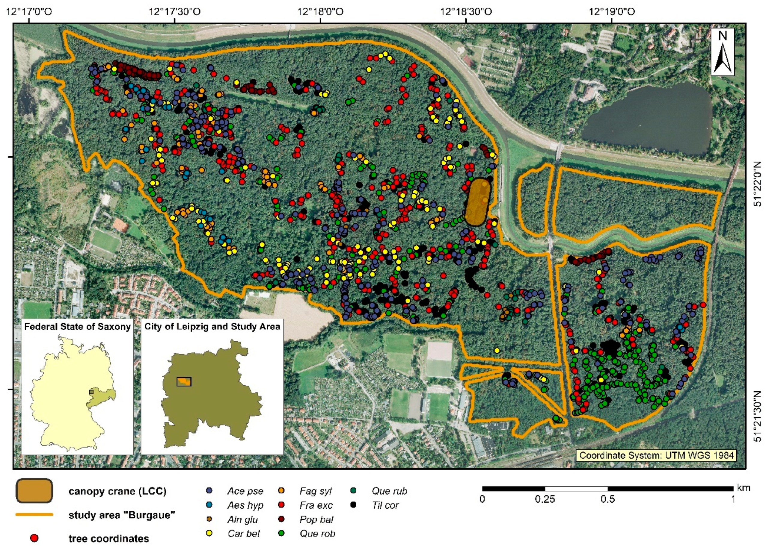
2.1. Study Site

The study site Burgaue is located within the city boundaries of Leipzig (Saxony, Germany) and covers a total area of 2.18 km² (see Figure 1). Situated in the floodplain of the Elster, Pleiße, and Luppe rivers, the Leipzig floodplain forest is one of the largest floodplain forests in Central Europe [38]. Leipzig lies in the transient zone of maritime and continental climate that is characterized by warm summers and an annual mean temperature of 8.4 °C with annual precipitation of 516 mm [39]. The study site is covered with a species-rich and structurally complex hardwood floodplain forest with European ash, English oak, Sycamore maple, European hornbeam, and Small-leaved lime being the dominant tree species [40]. Forest inventories provided species information and exact geolocation of a total of 1702 trees in the upper tree layer (Figure 1). Within the study site, a crane facility (Leipzig Canopy Crane facility, LCC) for the investigation of forest tree canopies was established in 2001. The crane facility covers a total area of 1.65 ha (Figure 1) and allows access to about 800 trees with a diameter at breast height (DBH) greater than 5 cm belonging to 17 different species, with Sycamore maple, European ash, and Small-leaved lime being the most dominant ones [41].

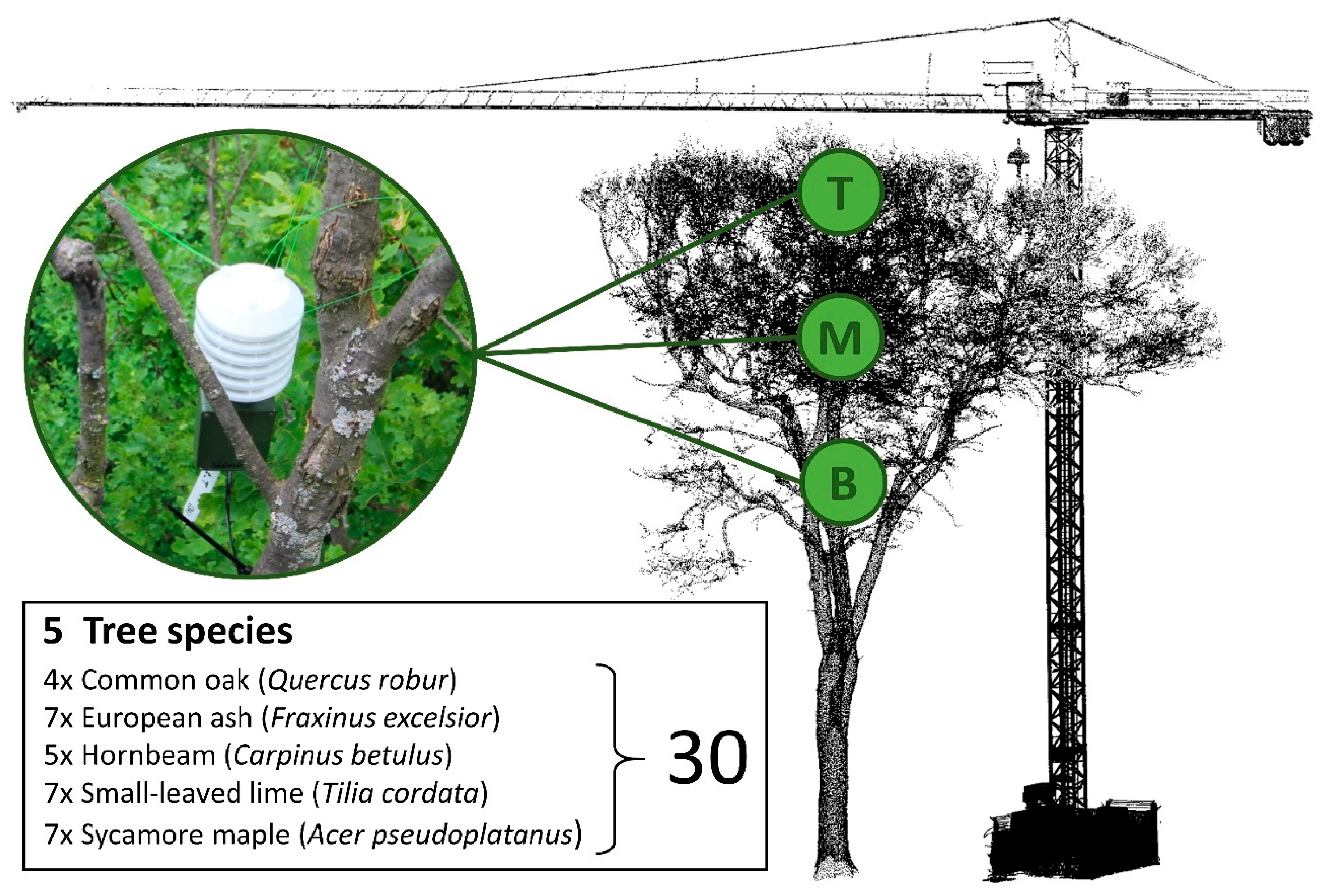
2.2. Measurement and Analysis of Air Temperatures within the Canopy

Tree crown air temperatures were measured at the crane site from July 1 to September 30 in 2016 for 30 randomly distributed old-growth tree individuals belonging to five different dominant tree species. In total, 90 temperature sensors (Scatter-100 DLTi/DLTc, UP Umweltanalytische Produkte GmbH, Ibbenbüren, Germany) were installed within the tree crowns (see Figure 2), with three sensors per tree at three different height layers in the tree crown (top, middle, bottom). The sensors recorded air temperatures at intervals of 10 min, resulting in 13,248 records for each sensor within the complete observation period. Species-specific differentiation of air temperatures was analyzed for each height layer and 10-min time interval separately, using a linear model of the form:

T_air = β₀ + β₁Height + β_2(j−1) Species_(j−1) + ε

(1)

with T_air being the response variable (air temperature in °C), Height being the sensor height above ground, in m, in the tree, Species being the species identity with j = {1, …, 5} levels, and ε being the error term. The sensor height was additionally included in the model to correct for species-specific height differences of the sensors. Based on these linear models, we additionally performed an ANOVA to test for the significance of the overall species effect. The estimates, as obtained from the linear model, and p-values of the species effect, resulting from the F-statistics in the ANOVA, were stored for subsequent analysis. Finally, we calculated, for all (144) possible 10-min intervals within a day, the proportion of models that found significant species effects for a specific daytime. If significant species effects on temperature were detected, estimates from the linear models were used to quantify the maximum interspecific temperature range. This procedure was repeated for each height layer (top, middle, bottom) separately. Due to existing missing values, we only modeled time steps with at least three available replicates per species.

2.3. Analysis of the Relationship between Tree Species and Surface Temperatures

We utilized forest inventory data from the LCC site and a preinstalled plot network consisting of 25 individual plots, each with a size of 2500 m². In all plots, trees were identified to the species level and tachymeter measurements were performed to determine the exact tree location. To increase the number of less-widespread species, additional field campaigns were realized with a differential GPS (Trimble Nomad^®900L, Trimble Ltd., Sunnyvale, CA, USA) to identify the exact geolocation. For all trees, the Kraft tree class indicating the social status of the trees in the stand [42] was identified to restrict further analysis to pre- and codominant trees, which were considered for the further analysis, resulting in a final sample size of 1702 tree individuals from 10 species (

Table 1. Available number of individuals per tree species to analyze effects on measured surface temperatures.

Scientific Name	Acronym	# of Individuals
Acer pseudoplatanus L.	Ace pse	156
Aesculus hippocastanum L.	Aes hyp	59
Alnus glutinosa (L.) Gaertn.	Aln glu	26
Carpinus betulus L.	Car bet	189
Fagus sylvatica L.	Fag syl	145
Fraxinus excelsior L.	Fra exc	338
Populus balsamifera L.	Pop bal	174
Quercus robur L.	Que rob	80
Quercus rubra L.	Que rub	75
Tilia cordata Mill.	Til cor	460

).

Tree crown surface temperatures were extracted from the thermal image data using (see Section 2.4) a buffer with a 3 m radius around the central coordinates of the target trees. The selected buffer diameter of 3 m corresponds to the crown diameter of temperate broadleaf tree species with a DBH of at least 40 cm [43]. All resulting pixel values were subsequently averaged according to their spatial coverage within the buffer. To test for significant species-related differences in mean surface temperatures, a spatial autocorrelation (SAC) model, as implemented in the R [44] package “spatialreg” [45] was applied, with species as grouping factor. The SAC model accounts for the presence of spatial autocorrelation not only in the response variable, but also in the random error term [46]. In order to test the overall species effect in the model, an additional null-model with permuted species identity was defined. Akaikie information criterion (AIC)-values [47] were used to assess model performance, whereby a decrease in AIC of two indicated an improvement of the candidate model in comparison to the null-model. To further test for differences of all possible species comparisons, each SAC model was recomputed, allowing each tree species (Table 1) being the reference category to be tested against.

To test in how far variations in crown surface temperatures may be paralleled to variations in canopy air temperatures, we used the subset of trees at the LCC site, as those were equipped with temperature sensors, and analyzed the statistical linkage via linear regression models. To this end, air temperatures measured at different height layers were averaged per tree individual for the time of the overflights. Due to missing values, five of 30 tree individuals had to be excluded from this analysis.

2.4. Remotely Sensed LST

2.4.1. Gyrocopter Data Acquisition and Preprocessing

An overflight was conducted with a gyrocopter platform (Cavalon D-MHSA, AutoGyro GmbH, Hildesheim, Germany) equipped with a thermal camera (VarioCAM hr, InfraTec, Dresden, Germany). The thermal camera was characterized by a resolution of 640 × 480 pixels and a field of view of 30°, thus providing, with a flight altitude of approximately 500 m a.g.l., a ground resolution of about 0.4 m. The flight was conducted under cloud-free conditions between 9:50–10:29 UTC (11:50–12:29 Central European Summer Time (CEST)) on 18 August in 2016, which was simultaneous to the overpass of the Landsat 8 satellite (10:02–10:03 UTC). The spectral response of the camera is in the range of 7.5–14 μm. At-sensor brightness temperatures were assessed by inverting Planck’s law. As the leaf level, emissivity within the 8–14 μm spectral range was found to vary between 0.94 and 0.98 for broadleaf tree species, converging against 1 with increasing sensor distance [48], and, as emissivities were unknown for the species in the study area, we assumed a constant emissivity of 1. A total of 182 individual thermal images were taken. The images were rectified and georeferenced and mosaicked to create an overall picture. The thermal camera was calibrated beforehand by means of a black body.

2.4.2. Landsat 8 Satellite Data—Products and Radiometric Processing

Landsat 8 multispectral and thermal imagery were downloaded through the United States Geological Survey (USGS) EarthExplorer interface (https://earthexplorer.usgs.gov). Multispectral Landsat 8 data were downloaded as atmospherically-corrected land surface reflectance product. Thermal imagery was used to derive LST following the method of Jiménez-Muñoz et al. [49], which calculates LST from at-sensor radiance by inverting Planck’s law while accounting for the contributions of atmospheric radiation transfer through a set of water vapor-dependent empirical atmospheric functions. Apart from at-sensor radiance, the method requires only two additional parameters: land surface emissivity and an estimate of atmospheric column water vapor. The atmospheric water vapor value (1.7 g × cm⁻²) was taken from the MODIS MOD05_L2 Product based on data collected from the Terra platform; data product files were provided by the Level 1 and Atmosphere Archive and Distribution System (LAADS) Distributed Active Archive Center (DAAC) (https://ladsweb.modaps.eosdis.nasa.gov). For a direct comparison with gyrocopter data, emissivity values were set to 1.0 across the image.

2.4.3. Statistical Downscaling of LST to Higher Spatial Resolution

Linear and nonlinear regression models between LST and ancillary remote-sensing-derived environmental predictors approximating compositional, structural, and environmental conditions have been widely established to enhance LST resolution [50,51,52]. Hutengs et al. [52] proposed a random forest (RF) [53]-based downscaling approach and showed it to outperform conventional methods such as the TsHARP sharpening approach [54]. We thus incorporated the proposed RF approach into our downscaling framework to achieve a spatially highly-resolved (30 m) LST product derived from the coarse resolution (100 m) Landsat 8 LST data. However, we adapted the predictor set to better reflect vegetation characteristics being relevant for a temperate floodplain forest. This set of predictors included surface reflectance data (blue, green, red, NIR, SWIR-1, SWIR-2) as well as a suite of spectral indices (

Table 2. Spectral indices used for downscaling of Landsat 8 land surface temperature (LST).

Acronym	Description	Formulation
NDVI	Normalized Difference Vegetation Index	$\frac{NIR-Red}{NIR+Red}$
NDWI	Normalized Difference Water Index	$\frac{NIR-SWIR1}{NIR+SWIR1}$
NMDI	Normalized Difference Moisture Index	$\frac{NIR-\left(SWIR1-SWIR2\right)}{NIR+\left(SWIR1-SWIR2\right)}$
GRVI	Green-Red Vegetation Index	$\frac{Green-Red}{Green+Red}$
NDDI	Normalized Difference Drought Index	$\frac{NDWI-NDVI}{NDWI+NDVI}$

), including

(1) Normalized Difference Vegetation Index (NDVI) [55], (2) Normalized Difference Water Index (NDWI) [56], (3) Normalized Multi-band Drought Index (NMDI) [57], (4) Green-Red Vegetation Index (GRVI) [58], and (5) Normalized Difference Drought Index (NDDI) [59]. NDVI and GRVI are related to biomass and structural parameters of the canopy [60,61,62], whereas NDWI, NMDI, and NDDI are rather sensitive to soil and canopy moisture content [56,57,59]. Based on their sensitivities, the selected indices may be specifically linked to, e.g., evapotranspiration and the canopy surface temperature.

The resulting LST product was subsequently validated via goodness of fit indices (R², RMSE, and SE) using the original gyrocopter-acquired high-resolution LST data, aggregated to the same spatial resolution as the downscaled LST product. To achieve more robust predictions of the goodness of fit statistics for the downscaling framework, we additionally performed a resampling approach with 1000 repetitions using 100 pixels that were randomly selected from the global LST image for each run.

3. Results

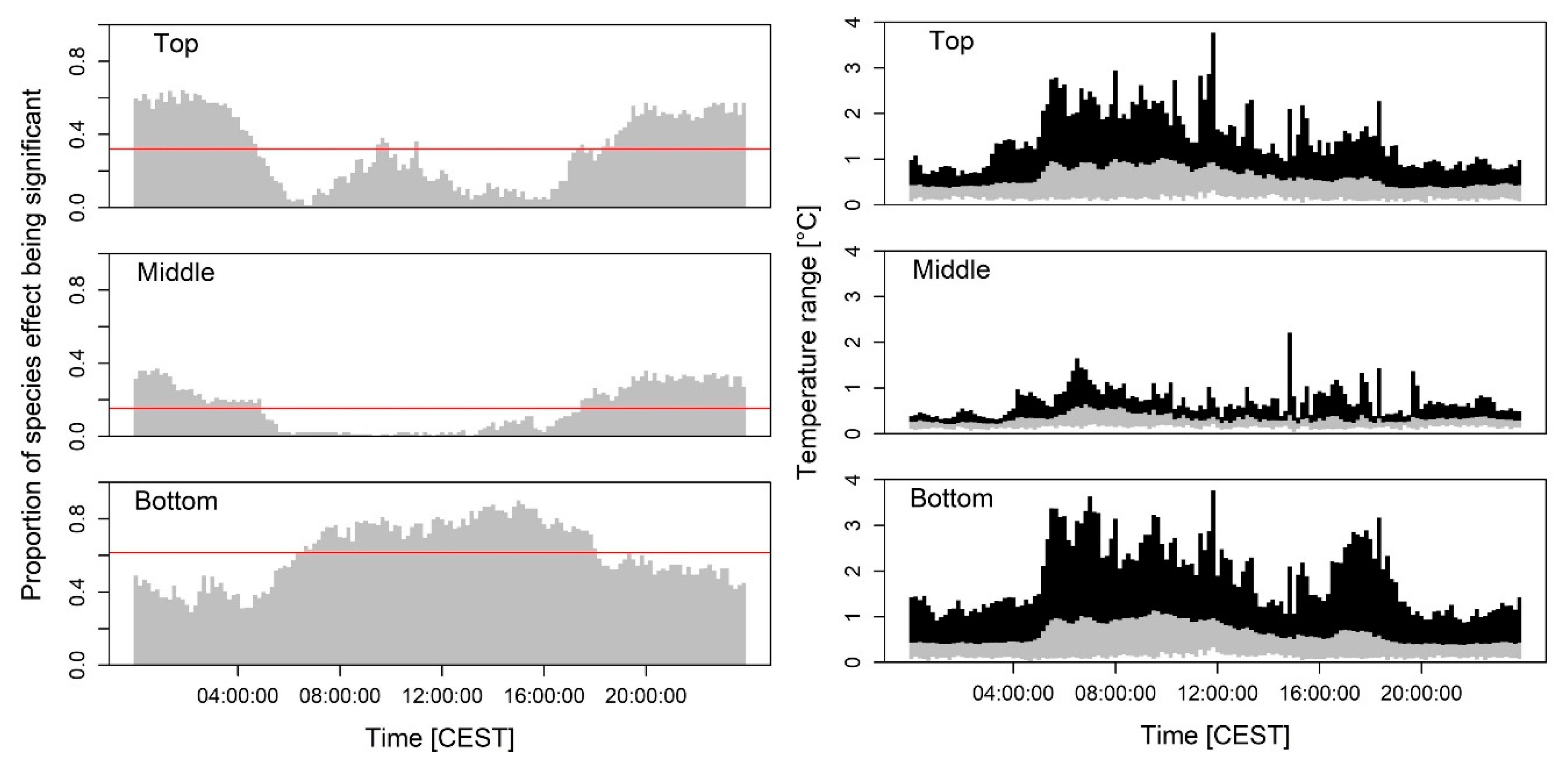
3.1. Species Effects on Crown Air Temperatures

Figure 3 summarizes the proportion of models finding significant tree species effects on air temperature and the corresponding range between tree species with highest and lowest air temperature for each of the three tree crown sensor positions (top, middle, bottom). Across all evaluated 10-min intervals, we found statistically significant temperature differences in the top layer in 32% of all intervals, in the middle layer in 15%, and in the bottom layer in 61%. Time periods with statistically significant temperature differences occurred more frequently and differed substantially between the tree layers. For the top layer, the time between 6 p.m. and 4 a.m. was most appropriate to detect species-specific temperature differences, with a second potentially suitable window between 9 a.m. and 12 a.m. In the middle layer, the period between 6 p.m. and 4 a.m. was also the most suitable, but statistically significant temperature differences were less frequent. Outside of this time window, no statistically significant temperature differences were observed in the middle layer. In the bottom layer, species-specific temperature differences could be detected throughout most of the day but were especially frequent in the period between 7 a.m. and 6 p.m.

The largest air-temperature variations occurred during midday in the top and bottom layers (~4 °C). Temperature differences in the top and bottom layers were substantially higher than in the middle layer and averaged about 1 °C in both layers. In the bottom layer, temperature differences were also slightly more pronounced than in the top layer.

In the top layer, which is visible to remote sensing instruments, the midday period, including noon, was generally not ideal for observing tree species-specific temperature differences detected by the sensor network. Nevertheless, we still found statistically significant tree species differences (p = 0.014) in mean crown air temperature for the time period (12:00–12:10 CEST) of the Landsat 8 overpass and the gyrocopter overflight.

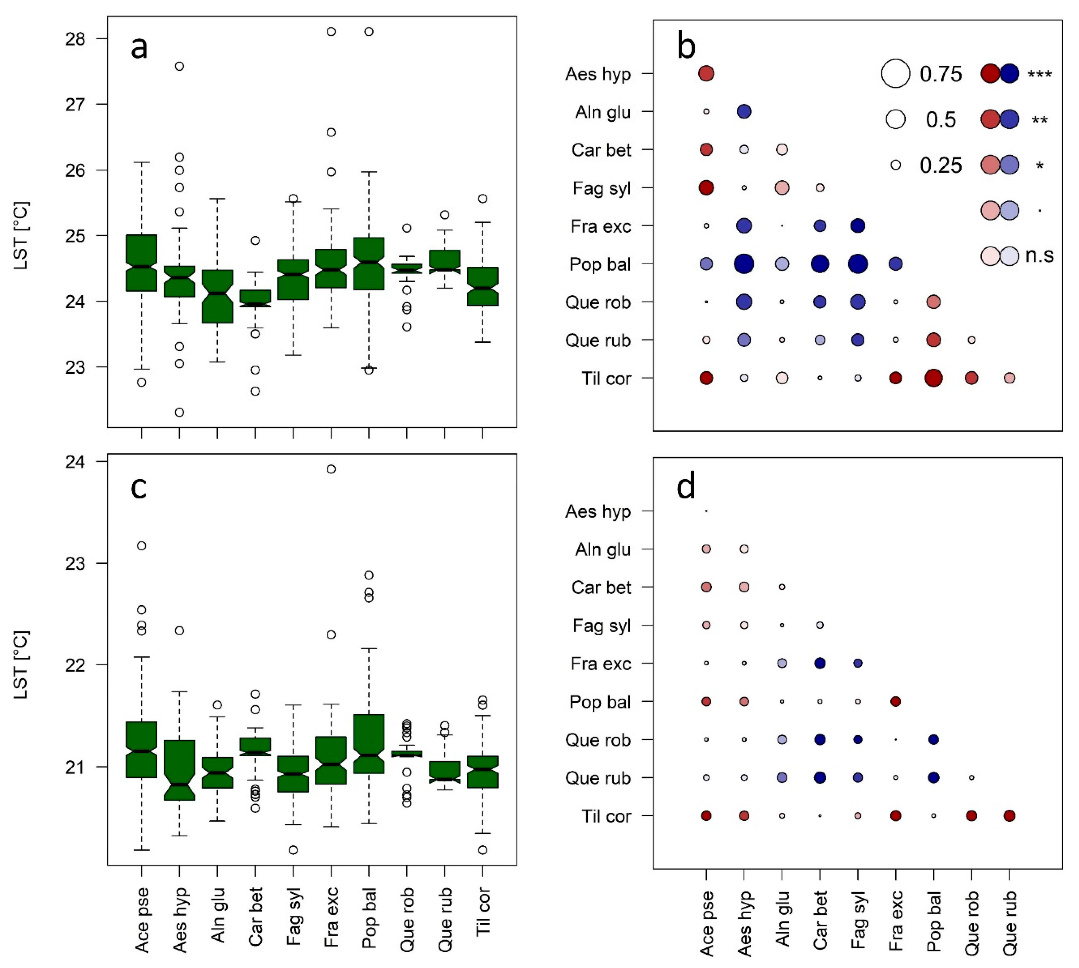
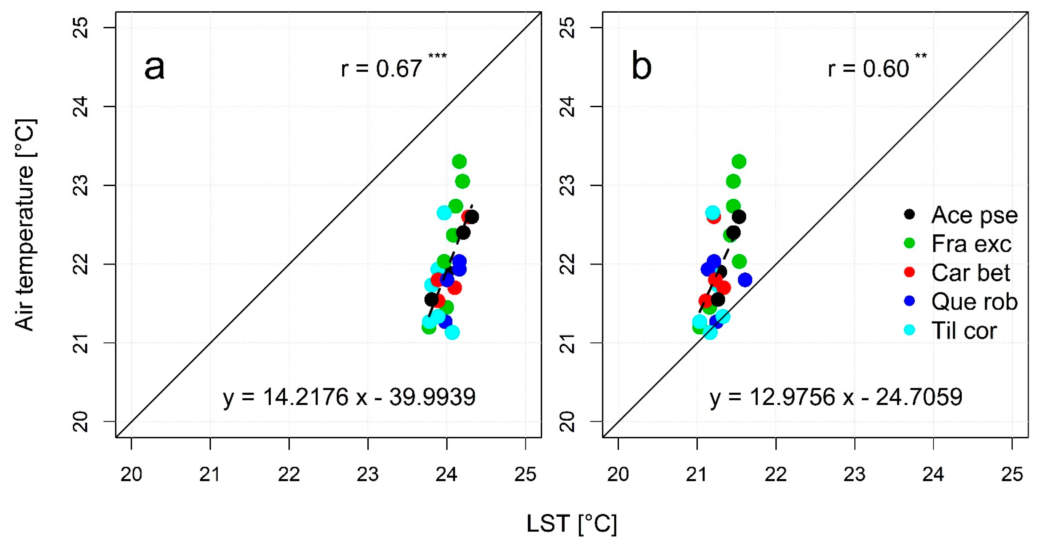
3.2. Fine-Scale Surface Temperatures from Gyrocopter Data: Linkages to Tree Species and Usage for the Modeling of Crown Air Temperatures

Based on the inventoried 1702 tree individuals all over the studied floodplain forest, we found only minor species-specific differences of LST as detected with the thermal camera onboard the gyrocopter platform (Figure 4a) The range between the species with highest and lowest median LST was at 1.07 °C. However, the plot documents a trend towards higher temperatures for the small-leaved species C. betulus, F. sylvatica and T. cordata usually found in drier habitats of the floodplain forest, compared to A. glutinosa, P. balsamifera and Q. robur. Intermediate crown temperatures were observed for the species A. pseudoplatanus and A. hippocastanum having the largest leaves among the tree species studied.

The SAC model that was used to test the overall tree species effect on surface temperatures improved considerably (ΔAIC = 79.88) over the null-model when considering species identity as predictor variable, which documents the statistical relevance of this attribute. For 56% of all tested species combinations (25/45), we found significant LST differences (Figure 4b). In particular P. balsamifera showed lower LST values than all other species. With the exception of A. glutinosa and Q. robur, these differences proved to be significant. In contrast, C. betulus showed higher LST values than all other species, whereas the differences towards T. cordata and F. sylvatica were very small, and thus not significant. However, due to the limited number of observations (n = 30), no significant species differences in LST were detectable when solely analyzing the species set present at the LCC site.

In the following, we tested, for the subset of species at the LCC site, whether observed LST variations may be of use to model canopy air temperatures. We found a linear relationship with a residual standard error (SE) of 0.51 °C (Figure 5), but Pearson’s r was moderate at 0.56 (p = 0.003). We also tested if the relationship between surface temperature and tree crown air temperature is tree species-specific, but no significant species effects on model slope and intercept were found (

Table 3. ANOVA table for the regression model testing gyrocopter LST at 0.4 m resolution and tree species identity, and their interaction, to predict air temperatures at the tree crown level; df = degrees of freedom, SS = sum of squares, F = F-value, p = p-value.

Predictor	df	SS	F	p
Gyro LST (0.4 m)	1	2.730	9.059	0.009
Species	4	0.837	0.695	0.607
Gyro LST (0.4 m): Species	4	0.556	0.461	0.763
Residuals	15	4.521

).

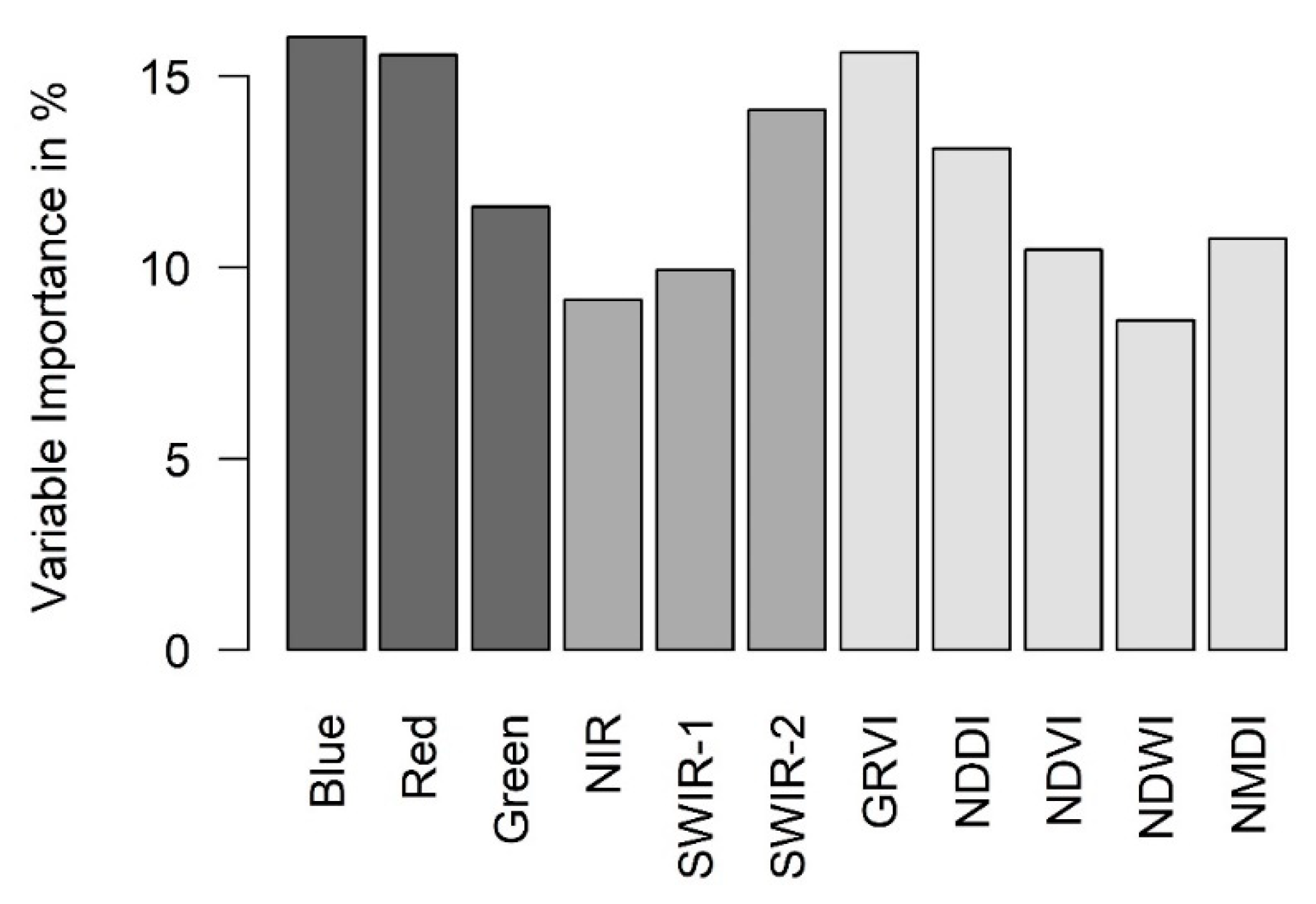
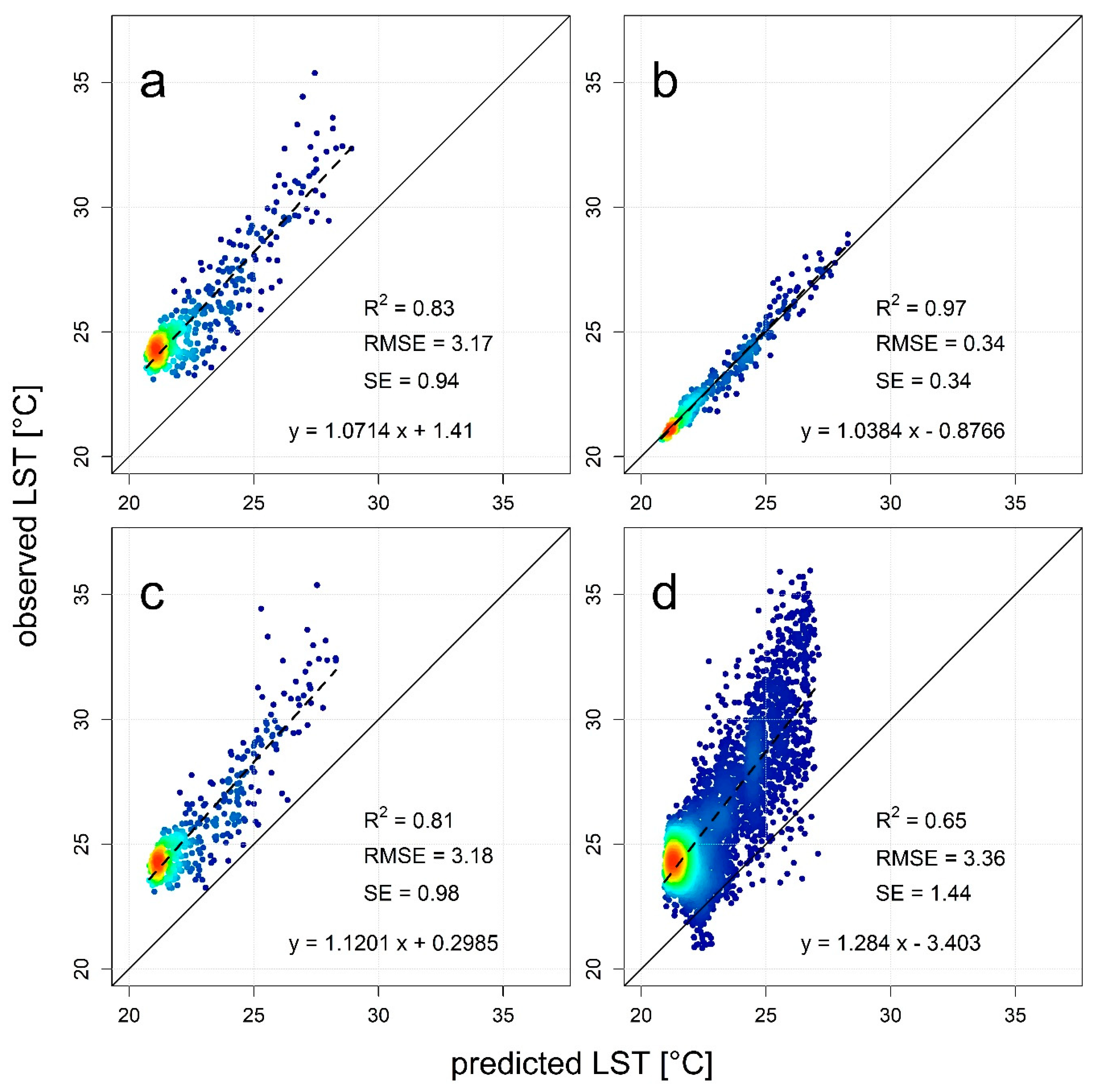
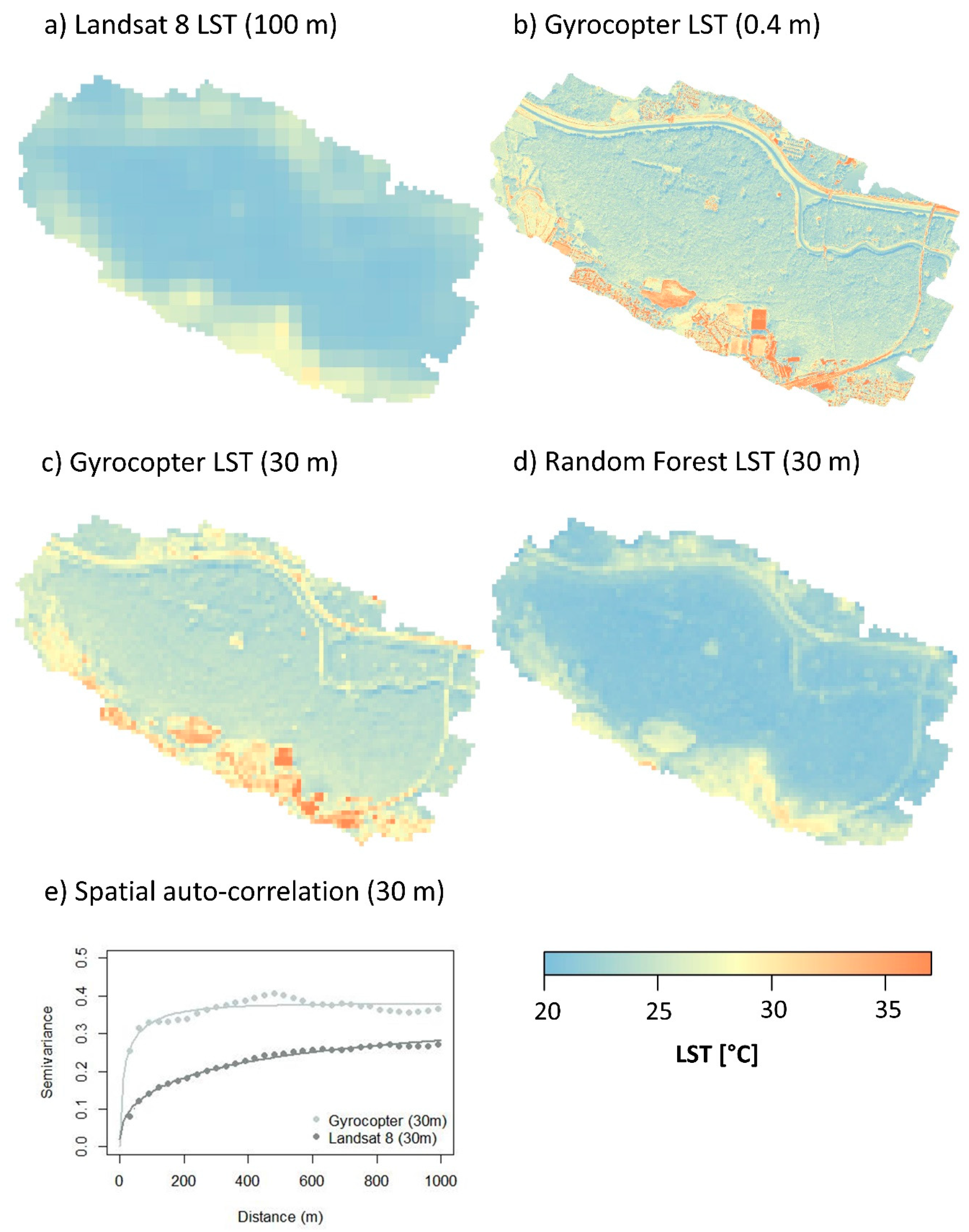
3.3. Downscaling for the Retrieval of 30-m LST Data

Landsat 8 LST data (100-m pixel size) matched well with gyrocopter-acquired LST data, the latter aggregated to the 100 m level; R² equaled 0.83 (Figure 7a). However, we found a bias of +1.41 °C for gyrocopter towards Landsat data, which induced a rather high RMSE of 3.17 °C. Parts of this bias may be traced back to different overflight times, with the gyrocopter flight lasting until ~12.30 CEST.

The calibrated random forest model (number of trees: 500; number of variables at each split: 4) was able to capture the existing LST variations in the Landsat image (100-m pixel size) almost fully (Figure 9a; R² = 0.97, RMSE = 0.34 °C). All variables contributed to the regression model, as indicated by the calculated variable importance (Figure 6). Overall, the visible domain proved to be of higher importance (mean = 14.39%) then the NIR to SWIR domain (mean = 11.06%) and the spectral indices (mean = 11.72%). However, it should be underlined that the magnitude, and also the ranking of the variable importance change, due to the intercorrelation among predictor variables when the set of variables considered in the model, is varied.

Comparison of RF-fitted Landsat LST values with aggregated gyrocopter LST provided similar results as with the original Landsat data: R² decreased slightly from 0.83 to 0.81, and RMSE and SE remained similarly stable (3.18 instead of 3.17 °C, and 0.98 °C instead of 0.94 °C; Figure 7a,c). The RF model, calibrated on the 100 m level, was then applied to predict LST values for a pixel size of 30 m. At this level, the comparison with aggregated gyrocopter data showed an R² value of 0.65, SE of 1.44 °C, and an RMSE of 3.36 °C, the latter mainly induced from the temperature bias between both datasets. Nevertheless, the temperature range reproduced in the downscaled Landsat data was more limited (~6.2 °C) than the range reproduced by gyrocopter data (~15.1 °C), which can be traced back to the limited temperature range within the original Landsat data and the interpolating (but not extrapolating) capacities of the calibrated RF model. For all spatial scales, R² and RMSE values reached in the internal validation with 100 randomly selected pixels (1000 bootstraps) were stable (low standard deviation given in brackets) and similar to those found for the complete (Figure 7) data (100 m: R² = 0.81 (0.04), RMSE = 3.17 (0.10), SE = 0.78 (0.07); 30 m: R² = 0.65 (0.07), RMSE = 3.36 (0.17), SE = 0.90 (0.08)). The SE, however, decreased markedly for both datasets, when being compared to the complete data.

The quality of the downscaled LST product (Figure 8) was further assessed by visual inspection. Small-scale variations in LST visible in the 0.4 m and 30 m gyrocopter datasets were, in general, well reproduced in the downscaled LST product. Nevertheless, prominent “hotspots” of LST and regions of higher variability, mainly in the south and southeast of the gyrocopter image, were not reproduced by downscaled Landsat data and appeared flat and without variation, but these areas were outside the forested areas.

As indicated by the analysis of the empirical semivariogram (Figure 8e), we overall found the spatial autocorrelation structure inherent in the gyrocopter data at the 30 m level to have an effective range (distance at 95% silt) of 210 m. For the downscaled LST product, the effective range of the spatial autocorrelation was, with 4264 m, found to be higher. The lower level of semivariance at a lag distance of 30 m observed for the downscaled LST product additionally indicates a reduced thermal contrast, compared to the gyrocopter data at the 30 m level.

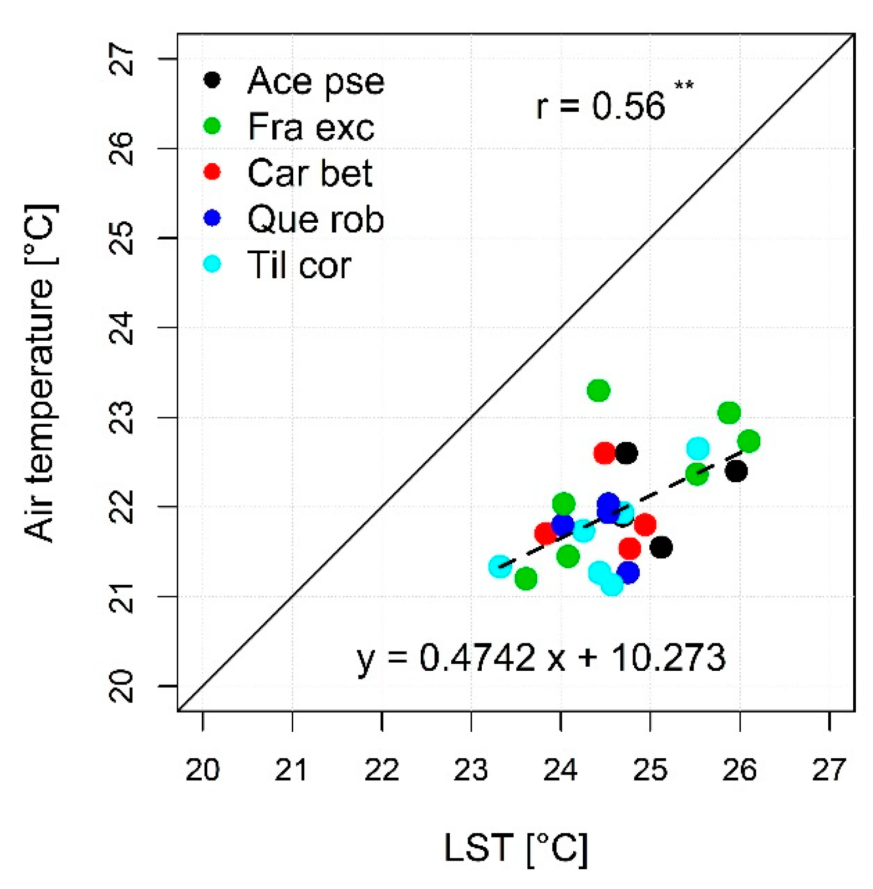
3.4. Detectability of Species-Specific Differences in LST and Air Temperature Based on Downscaled LS8 TIR Data

To further test the capability of the downscaled LST product at 30 m resolution to detect species-specific differences in surface temperature, it was benchmarked against the gyrocopter data at 0.4 m, and aggregated to 30 m spatial resolution. Overall, we found the ranking of tree species-specific LST well preserved across all datasets and spatial scales tested (Figure 4 and Figure 9), even though the temperature range between the warmest and the coolest tree species decreased with increasing spatial aggregation to 0.63 °C for the gyrocopter and to 0.33 °C for the downscaled Landsat 8 LST product, respectively. When comparing species-specific surface temperatures, inconsistency between gyrocopter-acquired LST and the downscaled Landsat 8 LST product was only pronounced for P. balsamifera, which was found to be among the tree species with lowest LST for the gyrocopter data at the 0.4 m and 30 m resolution, and among the tree species with highest LST for the downscaled LST product.

For the LST products at the 30 m level, species effects on surface temperature were slightly less pronounced in the SAC models (ΔAIC_Gyro30 = 68.3, ΔAIC_LS8 = 68.1), compared to the gyrocopter data at very high resolution (ΔAIC_Gyro0.4 = 79.88). Even though the interspecies comparison (Figure 9b,d) showed a clear underestimation of species-specific differences in surface temperature, compared to those observed with 0.4 m gyrocopter data (Figure 4b), qualitative interspecific differences remained stable for gyrocopter data at 0.4 m and 30 m resolution. Significant between-species differences in LST were detectable in 47% of all cases tested (21/45). However, qualitative patterns remained slightly more ambiguous when comparing the results achieved using the downscaled Landsat 8 product to those achieved using the gyrocopter data at 0.4 m and 30 m resolution. For the downscaled LS8 product, the percentage of finding significant interspecific differences in LST decreased to 44% (20/45). Especially for P. balsamifera and A. glutinosa, contrasting relationships were observed for the interspecific comparison of surface temperature differences, when being compared to the results achieved using the gyrocopter data at 0.4 m and 30 m resolution.

When linking variations in LST to canopy air temperatures (Figure 10), differences in Pearson’s r for gyrocopter LST at the 30 m level (r = 0.67, p < 0.001), the downscaled LST product (r = 0.6, p = 0.002), and the gyrocopter dataset at 0.4 m resolution (r = 0.56, p = 0.003) were found to be nonsignificant when compared among each other based on pairwise Steiger’s Z tests [63] (gyrocopter 0.4 m, gyrocopter 30 m (p = 0.52); gyrocopter 0.4 m, LS8 30 m (p = 0.84); gyrocopter 30 m, LS8 30 m (p = 0.63)). The achieved standard errors for the gyrocopter data at 30 m resolution (SE = 0.45 °C), the downscaled LST product (SE = 0.49 °C), and the high-resolution gyrocopter data (SE = 0.51 °C) were also found to be comparable across the different datasets. The relationship between surface and tree crown air temperatures contained no significant species effects on model slope and intercept (

Table 4. ANOVA table for the regression models testing gyrocopter LST at 30 m resolution or the downscaled Landsat 8 and tree species identity, and their interaction, to predict air temperatures at the tree crown level; df = degrees of freedom, SS = sum of squares, F = F-value, p = p-value.

Predictor	df	SS	F	p
Gyro LST (30 m)	1	3.910	22.900	<0.001
Species	4	1.101	1.612	0.223
Gyro LST (30 m): Species	4	1.072	1.570	0.233
Residuals	15	2.561
LS8 LST (30 m)	1	3.112	12.413	0.003
Species	4	0.494	0.492	0.741
LS8 LST (30 m): Species	4	1.277	1.273	0.324
Residuals	15	3.761

).

4. Discussion

4.1. Spatial and Temporal Dependency of the Tree Species-Specific Modulation of Air Temperatures

Numerous studies have shown that characteristics of tree species, such as tree morphological and physiological characteristics including transpiration rates, canopy size, and canopy density, as well as features of tree leaves, can influence cooling effect of trees [13,21,35,64]. However, how far air temperature varies within tree crowns and between different tree species remains unsolved so far. The results obtained from the sensor network used in this study support the hypothesized temporal and spatial variability, whereby the mean differences between coldest and warmest tree species equaled 1 °C and reached maxima of up to 4 °C for the upper and lower canopy region. This is, at its maxima, in the same range as the considered overall cooling potential of vegetation [7,9,34], and at its mean, close to the forecast rise in temperature of 1.5 °C caused by global warming [65]. Nevertheless, we observed a reduced likelihood to detect a differentiation in canopy air temperature towards the top of the tree crown, which is more closely coupled to the atmosphere. Rahman et al. [13] showed that canopy density, sap flow, and soil moisture interact in a complex way to provide a distinctive cooling effect. Tree transpiration rates and thus latent heat flux were, however, found to be species-specific [66], and overall higher for sunlit leaves at the top of the canopy [67]. The pronounced diurnal differences in canopy temperature observed at the top of the canopy are thus driven by differences of latent, rather than of sensible, heat flux. Differently, species-specific air temperature differences at the bottom layer are likely arising from a variation in shading, caused by differences in canopy architecture and transparency [13,68]. The small, but frequently observed, nocturnal between-species differences in air temperature are potentially due to variations in sensible heat fluxes that can be traced back to different thermal heat storage capacities and conductivities depending on the moisture content and other biophysical properties of leaves and woody material [69,70]. Schultz et al. [26], however, found nocturnal temperature differences at larger spatial scales only partially to be explained by daytime surface load. Night-time evapotranspiration as an alternative explanation seems to be less likely, as relevant transpiration rates during that time of the day were only observed for early successional tree species [71], e.g., Populus spec. The observed reduced likelihood of finding significant species differences in canopy air temperature during daytime may also be traced back to the thermal mixing, which arises from a steep vertical temperature gradient, that is less pronounced at night [10]. The layer between the top canopy which is fully exposed to the incoming radiation and the well-shaded bottom of the canopy is characterized by thermal turbulences, cancelling out significant between-species differences in air temperature at the middle position of the tree crown. As a consequence of all these effects, canopy temperatures cannot be explained in a straightforward manner. However, we proved that tree species modulate the within-canopy air temperature differently, and that the order of observed between-species differences is large enough to be biologically relevant [72,73].

4.2. Usefulness of High-Resolution Remote Sensing Data for Monitoring Species Effects on Surface Temperature and the Modeling of Air Temperature

We also observed a tendency of small-leaved species towards higher canopy surface temperatures, which is in line with the findings of Leutzinger et al. [35]. Beyond purely morphological effects, differences of transpiration were found, for example by Monteiro et al. [74], to be also highly relevant for regulating leaf temperatures. This was also present in our study, as we observed a trend of isohydric trees with intermediate leaf sizes, adapted to moist habitat (e.g., A. glutinosa, P. balsamifera) towards lower surface temperatures. Leutzinger et al. [35] reported between-species differences in surface temperature of ~3 °C for park trees. Our analysis provided minor species differences of ~1 °C, which may be, in part, traced back to abnormally dry to moderate drought soil conditions with limited evapotranspiration rates, reported by the Drought Monitor Germany [75] for our study site and investigation period. It is still debated to what extent drought conditions result in an equalization of species-specific surface temperatures. For example, McGloin et al. [76] and Schwaab et al. [14] found an opposite tendency when comparing broadleaf and needleleaf tree species. Compared to the findings of Leutzinger et al. [35], we also observed a larger intraspecific variability in surface temperature of up to 6 °C, thus hampering the detectability of tree species differences. This variability presumably resulted from varying transpiration rates caused by small-scale variations in water supply (e.g., rooting depth in relationship to groundwater table) or potentially also by varying degrees of tree vitality [77,78]. We tried to account for potential effects of a systematic variation in environmental gradients on the detected species differences in surface temperature by trying to ensuring an unclustered spatial design of the focal tree species and by explicitly taking spatial autocorrelation into account using the SAC model.

Several studies have investigated differences between air temperature and surface temperature using a combination of in situ and remote sensing measurements [79,80]. Canopy surface temperatures were found to vary rapidly with meteorological and plant physiological conditions, while responses in air temperature occurred slower and were less severe [36,81]. During the night, linkages between both are close, while the relationship at daytime is more complex and strongly impacted by differences in land use and cover [36,81]. Despite this, variations in surface temperature measured at canopy level were found to be significantly correlated (r = 0.56, SE = 0.51 °C) to mean canopy air temperatures across tree species tested in this study with a mono-temporal approach. It has been shown that the magnitude of surface to air temperature differences (ΔT) varies with the energy exchanges in the form of sensible and latent heat [81], but also with the spatial resolution of the LST data used [30]. Leutzinger and Körner [21] found the species ranking in ΔT, however, well preserved when analyzing time series of close-range TIR data. We thus consider high-resolution LST data a valuable data source to predict species-specific small-scale variations in air temperature at the tree crown level, although addressing the variation in ΔT at the whole crown level and across crown layers needs to receive further attention.

4.3. Transferabilty to Satelite-Derived LST Measurements

Routine observations of species-specific temperature differences and analyses on larger spatial scales are challenging to get realized with high-resolution overflights. We therefore evaluated if species-specific temperature differences could also be mapped at the Landsat scale with temperature data fields downscaled from native Landsat 8 100 m thermal data to the 30 m spatial resolution corresponding to its reflectance bands.

Downscaled Landsat 8 LSTs gave satisfactory results overall, comparable to other downscaling studies in terms of explained variation at the fine scale [82,83]. However, the visual detailedness in the downscaled imagery was lower than for the gyrocopter LST data aggregated to 30 m, and exhibited a higher degree of spatial dependency. The residual correction step of the downscaling model, which ensures unbiased LST estimates across spatial scales against the original 100 m input data, is likely the leading cause of this effect [52]. Absolute LST values also showed a substantial bias between downscaled Landsat 8 data and gyrocopter LST at the 30 m level. The relatively high RMSE (~3 °C) of the downscaled Landsat 8 product, compared to the gyrocopter data, could largely be attributed to a systematic temperature bias between both sensors (~1.4 °C), which is furthermore underpinned by the low SE (0.9 °C) achieved in the internal validation. A similar thermal offset between downscaled Landsat TM data and high-resolution airborne data (~30 m) was previously demonstrated, for example, by Bonafoni et al. [82]. Such differences typically arise due to mismatches in overpass times between sensors. As we specifically controlled for overpass time by carrying out the gyrocopter observations concurrent with the Landsat 8 overpass, thermal sensor band positions and different atmospheric paths probably caused the temperature offset. Importantly, such a systematic offset will not affect comparisons of species-specific LST differences as long as it is constant across the image, as was the case here, but could be corrected with an inter-sensor calibration at the coarse scale [52,84]. Despite the outlined limitations of downscaled Landsat 8 thermal imagery, we found that the species ranking by LST was well-preserved in the downscaled 30 m LSTs, and comparable to the gyrocopter data irrespective of their spatial resolution (0.4 and 30 m).

The reduction in thermal contrast at 30 m spatial aggregation resulted in a lower between-species LST range, especially for the downscaled LST product. While this affected the detection of species effects on LST, the detectability of between-species differences remained largely unchanged for the gyrocopter data at the 30 m level. The magnitude of between-species LST differences was reduced, however, compared to the high-resolution gyrocopter data.

Our findings indicate, contrary to former assumptions [21,36], that a species-specific signal on LST can be sufficiently preserved at the typical scale of remote sensing observations, despite the mismatch between target object size and pixel resolution. Our analysis of the correlations between crown air-temperature measurements, downscaled Landsat data (r = 0.60, SE = 0.49), airborne data aggregated to the 30 m (r = 0.67, SE = 0.47), and airborne data at 0.4 m resolution (r = 0.56, SE = 0.51) showed no statistically significant differences, but still indicated that the 30-m airborne data was capable of representing tree crown temperatures better than the high-resolution data. Air temperatures represent an integrated measurement of heat fluxes within the canopy and its immediate neighborhood. Miller et al. [10], for example, reported significant effects of canopy gaps on the ventilation of air and thus the below-canopy air temperature regime. Accordingly, LSTs at the 30 m scale might be appropriate to model air temperatures at the crown scale. The correlations we found between LST and air temperature over our study site were also similar to those observed in other studies at larger spatial scales [22,85,86]. Taken together, this suggests that routine satellite observations combined with LST downscaling algorithms could be capable of analyzing tree species–air temperature interactions at local and regional scales. However, as the cooling potential of vegetation at the larger spatial scale is strongly influenced by environmental gradients [8,14], additional predictors removing the impact of topography and other environmental characteristics on the temperature signal should be taken into consideration when analyzing tree species effects on forest temperatures.

5. Conclusions

In the present study, we analyzed the effects of tree species on air temperature variation in a floodplain forest stand through the integration of in situ temperature sensor networks and remote sensing observations from airborne and satellite sensors.

Our findings underline the coupling of air temperatures and tree species composition within forest stands, as temperature modulations of up to ~4 °C can be observed over short distances at the local study site. We further showed that these modulations can be linked to remotely-sensed surface temperatures, either at the scale of high-resolution airborne sensors (~1 m) or routine observations from satellite platforms (~30 m), and demonstrated that observation time is an important consideration when trying to detect species-specific temperature differences.

Observing surface temperature variations in forest stands with remotely-sensed data can, therefore, complement local sensor networks through detailed spatial analysis of, for example, tree species-specific responses to environmental variations (e.g., drought) or the effects of tree species composition, structural, and functional diversity on the microclimatic buffering capacity of forest stands [8]. Unlike sensor networks, airborne or satellite observations cannot provide a three-dimensional representation of air temperature fields in forest stands, e.g., vertical temperature variation, in the form of continuous time series measurements. Accordingly, the use of thermal imagery to map tree species-specific temperature variations may prove especially beneficial over larger spatial scales or in remote locations where permanent sensor networks cannot be readily established. Given the restrictions of high-resolution airborne sensor observations (costs, scheduling) and the limitations of current routine satellite thermal imagery in terms of spatial resolution (~100–1000 m), downscaling algorithms could provide an efficient strategy to fill potential data gaps and thus complement existing frameworks [14,15] to analyze the effects of vegetation characteristics on the surface energy balance at larger spatial scales and at larger areas.

References

1. Ryan, M.G. Temperature and tree growth. Tree Physiol. 2010, 30, 667–668. [Google Scholar] [CrossRef] [PubMed] [Green Version]
2. Nievola, C.C.; Carvalho, C.P.; Carvalho, V.; Rodrigues, E. Rapid responses of plants to temperature changes. Temperature (Austin) 2017, 4, 371–405. [Google Scholar] [CrossRef] [PubMed]
3. Joly, F.-X.; Milcu, A.; Scherer-Lorenzen, M.; Jean, L.-K.; Bussotti, F.; Dawud, S.M.; Müller, S.; Pollastrini, M.; Raulund-Rasmussen, K.; Vesterdal, L.; et al. Tree species diversity affects decomposition through modified micro-environmental conditions across European forests. New Phytol. 2017, 214, 1281–1293. [Google Scholar] [CrossRef] [PubMed] [Green Version]
4. Kim, Y.; Still, C.J.; Hanson, C.V.; Kwon, H.; Greer, B.T.; Law, B.E. Canopy skin temperature variations in relation to climate, soil temperature, and carbon flux at a ponderosa pine forest in central Oregon. Agric. For. Meteorol. 2016, 226–227, 161–173. [Google Scholar] [CrossRef] [Green Version]
5. Van Dijk, A.I.J.M.; Dolman, A.J.; Schulze, E.-D. Radiation, temperature, and leaf area explain ecosystem carbon fluxes in boreal and temperate European forests. Glob. Biogeochem. Cycles 2005, 19. [Google Scholar] [CrossRef]
6. Rahman, M.A.; Moser, A.; Rötzer, T.; Pauleit, S. Microclimatic differences and their influence on transpirational cooling of Tilia cordata in two contrasting street canyons in Munich, Germany. Agric. For. Meteorol. 2017, 232, 443–456. [Google Scholar] [CrossRef]
7. Rahman, M.A.; Moser, A.; Rötzer, T.; Pauleit, S. Within canopy temperature differences and cooling ability of Tilia cordata trees grown in urban conditions. Build. Environ. 2017, 114, 118–128. [Google Scholar] [CrossRef]
8. De Frenne, P.; Zellweger, F.; Rodríguez-Sánchez, F.; Scheffers, B.R.; Hylander, K.; Luoto, M.; Vellend, M.; Verheyen, K.; Lenoir, J. Global buffering of temperatures under forest canopies. Nat. Ecol. Evol. 2019, 3, 744–749. [Google Scholar] [CrossRef]
9. Rahman, M.A.; Stratopoulos, L.M.; Moser-Reischl, A.; Zölch, T.; Häberle, K.-H.; Rötzer, T.; Pretzsch, H.; Pauleit, S. Traits of trees for cooling urban heat islands: A meta-analysis. Build. Environ. 2020, 170, 106606. [Google Scholar] [CrossRef]
10. Miller, S.D.; Goulden, M.L.; da Rocha, H.R. The effect of canopy gaps on subcanopy ventilation and scalar fluxes in a tropical forest. Agric. For. Meteorol. 2007, 142, 25–34. [Google Scholar] [CrossRef] [Green Version]
11. Kovács, B.; Tinya, F.; Ódor, P. Stand structural drivers of microclimate in mature temperate mixed forests. Agric. For. Meteorol. 2017, 234–235, 11–21. [Google Scholar] [CrossRef] [Green Version]
12. Ehbrecht, M.; Schall, P.; Ammer, C.; Seidel, D. Quantifying stand structural complexity and its relationship with forest management, tree species diversity and microclimate. Agric. For. Meteorol. 2017, 242, 1–9. [Google Scholar] [CrossRef]
13. Rahman, M.A.; Moser, A.; Rötzer, T.; Pauleit, S. Comparing the transpirational and shading effects of two contrasting urban tree species. Urban Ecosyst. 2019, 22, 683–697. [Google Scholar] [CrossRef]
14. Schwaab, J.; Davin, E.L.; Bebi, P.; Duguay-Tetzlaff, A.; Waser, L.T.; Haeni, M.; Meier, R. Increasing the broad-leaved tree fraction in European forests mitigates hot temperature extremes. Sci. Rep. 2020, 10, 14153. [Google Scholar] [CrossRef] [PubMed]
15. Duveiller, G.; Hooker, J.; Cescatti, A. The mark of vegetation change on Earth’s surface energy balance. Nat. Commun. 2018, 9, 679. [Google Scholar] [CrossRef] [PubMed] [Green Version]
16. Janssen, P.; Fuhr, M.; Bouget, C. Beyond forest habitat qualities: Climate and tree characteristics as the major drivers of epiphytic macrolichen assemblages in temperate mountains. J. Veg. Sci. 2019, 30, 42–54. [Google Scholar] [CrossRef] [Green Version]
17. Lindo, Z.; Winchester, N. Out on a limb: Microarthropod and microclimate variation in coastal temperate rainforest canopies. Insect Conserv. Divers. 2013, 6, 513–521. [Google Scholar] [CrossRef]
18. Keenan, T.F.; Richardson, A.D.; Hufkens, K. On quantifying the apparent temperature sensitivity of plant phenology. New Phytol. 2020, 225, 1033–1040. [Google Scholar] [CrossRef] [Green Version]
19. Lin, Y.-S.; Medlyn, B.E.; Ellsworth, D.S. Temperature responses of leaf net photosynthesis: The role of component processes. Tree Physiol. 2012, 32, 219–231. [Google Scholar] [CrossRef] [Green Version]
20. Simon, H.; Lindén, J.; Hoffmann, D.; Braun, P.; Bruse, M.; Esper, J. Modeling transpiration and leaf temperature of urban trees—A case study evaluating the microclimate model ENVI-met against measurement data. Landsc. Urban Plan. 2018, 174, 33–40. [Google Scholar] [CrossRef]
21. Leuzinger, S.; Körner, C. Tree species diversity affects canopy leaf temperatures in a mature temperate forest. Agric. For. Meteorol. 2007, 146, 29–37. [Google Scholar] [CrossRef]
22. Mildrexler, D.J.; Zhao, M.; Running, S.W. A global comparison between station air temperatures and MODIS land surface temperatures reveals the cooling role of forests. J. Geophys. Res. 2011, 116, 245. [Google Scholar] [CrossRef]
23. Mutiibwa, D.; Strachan, S.; Albright, T. Land Surface Temperature and Surface Air Temperature in Complex Terrain. IEEE J. Sel. Top. Appl. Earth Obs. Remote Sens. 2015, 8, 4762–4774. [Google Scholar] [CrossRef]
24. Song, J.; Wang, Z.-H.; Myint, S.W.; Wang, C. The hysteresis effect on surface-air temperature relationship and its implications to urban planning: An examination in Phoenix, Arizona, USA. Landsc. Urban Plan. 2017, 167, 198–211. [Google Scholar] [CrossRef]
25. Serra, C.; Lana, X.; Martínez, M.D.; Roca, J.; Arellano, B.; Biere, R.; Moix, M.; Burgueño, A. Air temperature in Barcelona metropolitan region from MODIS satellite and GIS data. Appl. Clim. 2020, 139, 473–492. [Google Scholar] [CrossRef]
26. Schultz, N.M.; Lawrence, P.J.; Lee, X. Global satellite data highlights the diurnal asymmetry of the surface temperature response to deforestation. J. Geophys. Res. Biogeosci. 2017, 122, 903–917. [Google Scholar] [CrossRef]
27. Yang, Y.; Cai, W.; Yang, J. Evaluation of MODIS Land Surface Temperature Data to Estimate Near-Surface Air Temperature in Northeast China. Remote Sens. 2017, 9, 410. [Google Scholar] [CrossRef] [Green Version]
28. Benali, A.; Carvalho, A.C.; Nunes, J.P.; Carvalhais, N.; Santos, A. Estimating air surface temperature in Portugal using MODIS LST data. Remote Sens. Environ. 2012, 124, 108–121. [Google Scholar] [CrossRef]
29. Schwarz, N.; Schlink, U.; Franck, U.; Großmann, K. Relationship of land surface and air temperatures and its implications for quantifying urban heat island indicators—An application for the city of Leipzig (Germany). Ecol. Indic. 2012, 18, 693–704. [Google Scholar] [CrossRef]
30. Kawashima, S.; Ishida, T.; Minomura, M.; Miwa, T. Relations between Surface Temperature and Air Temperature on a Local Scale during Winter Nights. J. Appl. Meteor. 2000, 39, 1570–1579. [Google Scholar] [CrossRef]
31. Ca, V.T.; Asaeda, T.; Abu, E.M. Reductions in air conditioning energy caused by a nearby park. Energy Build. 1998, 29, 83–92. [Google Scholar] [CrossRef]
32. Prihodko, L.; Goward, S.N. Estimation of air temperature from remotely sensed surface observations. Remote Sens. Environ. 1997, 60, 335–346. [Google Scholar] [CrossRef]
33. Zhang, R.; Zhou, Y.; Yue, Z.; Chen, X.; Cao, X.; Ai, X.; Jiang, B.; Xing, Y. The leaf-air temperature difference reflects the variation in water status and photosynthesis of sorghum under waterlogged conditions. PLoS ONE 2019, 14, e0219209. [Google Scholar] [CrossRef] [PubMed] [Green Version]
34. Qiu, G.; Li, H.; Zhang, Q.; Chen, W.; Liang, X.; Li, X. Effects of Evapotranspiration on Mitigation of Urban Temperature by Vegetation and Urban Agriculture. J. Integr. Agric. 2013, 12, 1307–1315. [Google Scholar] [CrossRef]
35. Leuzinger, S.; Vogt, R.; Körner, C. Tree surface temperature in an urban environment. Agric. For. Meteorol. 2010, 150, 56–62. [Google Scholar] [CrossRef]
36. Zellweger, F.; de Frenne, P.; Lenoir, J.; Rocchini, D.; Coomes, D. Advances in Microclimate Ecology Arising from Remote Sensing. Trends Ecol. Evol. 2019, 34, 327–341. [Google Scholar] [CrossRef] [PubMed] [Green Version]
37. Hulley, G.C.; Ghent, D.; Hook, S.J. A Look to the Future: Thermal-Infrared Missions and Measurements. In Taking the Temperature of the Earth: Steps towards Integrated Understanding of Variability and Change, 1st ed.; Elsevier: Amsterdam, The Netherlands, 2019; pp. 227–237. ISBN 9780128144589. [Google Scholar]
38. Haase, D.; Gläser, J. Determinants of floodplain forest development illustrated by the example of the floodplain forest in the District of Leipzig. For. Ecol. Manag. 2009, 258, 887–894. [Google Scholar] [CrossRef]
39. Jansen, E. Das Naturschutzgebiet Burgaue; Staatliches Umweltfachamt: Leipzig, Germany, 1999. [Google Scholar]
40. Richter, R.; Reu, B.; Wirth, C.; Doktor, D.; Vohland, M. The use of airborne hyperspectral data for tree species classification in a species-rich Central European forest area. Int. J. Appl. Earth Obs. Geoinf. 2016, 52, 464–474. [Google Scholar] [CrossRef]
41. Patzak, R.; Richter, R.; Engelmann, R.A.; Wirth, C. Tree crowns as meeting points of diversity generating mechanisms—A test with epiphytic lichens in a temperate forest. bioRxiv 2020. [Google Scholar] [CrossRef] [Green Version]
42. Zawieja, B.; Kaźmierczak, K. Allocation of oaks to Kraft classes based on linear and nonlinear kernel discriminant variables. Biometr. Lett. 2016, 53, 37–46. [Google Scholar] [CrossRef]
43. Hemery, G.E.; Savill, P.S.; Pryor, S.N. Applications of the crown diameter–stem diameter relationship for different species of broadleaved trees. For. Ecol. Manag. 2005, 215, 285–294. [Google Scholar] [CrossRef]
44. R Core Team. R: A Language and Environment for Statistical Computing; R Foundation for Statistical Computing: Vienna, Austria, 2020; Available online: https://www.R-project.org/ (accessed on 28 December 2020).
45. Bivand, R.; Piras, G. Comparing Implementations of Estimation Methods for Spatial Econometrics. J. Stat. Soft. 2015, 63. [Google Scholar] [CrossRef] [Green Version]
46. Song, C.; Kwan, M.-P.; Song, W.; Zhu, J. A Comparison between Spatial Econometric Models and Random Forest for Modeling Fire Occurrence. Sustainability 2017, 9, 819. [Google Scholar] [CrossRef] [Green Version]
47. Akaike, H. A new look at the statistical model identification. IEEE Trans. Autom. Contr. 1974, 19, 716–723. [Google Scholar] [CrossRef]
48. Ribeiro da Luz, B.; Crowley, J.K. Spectral reflectance and emissivity features of broad leaf plants: Prospects for remote sensing in the thermal infrared (8.0–14.0 μm). Remote Sens. Environ. 2007, 109, 393–405. [Google Scholar] [CrossRef]
49. Jimenez-Munoz, J.C.; Sobrino, J.A.; Skokovic, D.; Mattar, C.; Cristobal, J. Land Surface Temperature Retrieval Methods from Landsat-8 Thermal Infrared Sensor Data. IEEE Geosci. Remote Sens. Lett. 2014, 11, 1840–1843. [Google Scholar] [CrossRef]
50. Yang, Y.; Cao, C.; Pan, X.; Li, X.; Zhu, X. Downscaling Land Surface Temperature in an Arid Area by Using Multiple Remote Sensing Indices with Random Forest Regression. Remote Sens. 2017, 9, 789. [Google Scholar] [CrossRef] [Green Version]
51. Wu, H.; Li, W. Downscaling Land Surface Temperatures Using a Random Forest Regression Model with Multitype Predictor Variables. IEEE Access 2019, 7, 21904–21916. [Google Scholar] [CrossRef]
52. Hutengs, C.; Vohland, M. Downscaling land surface temperatures at regional scales with random forest regression. Remote Sens. Environ. 2016, 178, 127–141. [Google Scholar] [CrossRef]
53. Breiman, L. Random Forests. Mach. Learn. 2001, 45, 5–32. [Google Scholar] [CrossRef] [Green Version]
54. Agam, N.; Kustas, W.P.; Anderson, M.C.; Li, F.; Neale, C.M. A vegetation index based technique for spatial sharpening of thermal imagery. Remote Sens. Environ. 2007, 107, 545–558. [Google Scholar] [CrossRef]
55. Rouse, J.W.; Haas, R.H.; Schell, J.A.; Deering, D.W. Monitoring vegetation systems in the Great Plains with ERTS. In 3rd ERTS Syposium, NASA SP-351 I; NASA: Washington, DC, USA, 1973; pp. 309–317. [Google Scholar]
56. Gao, B. NDWI—A normalized difference water index for remote sensing of vegetation liquid water from space. Remote Sens. Environ. 1996, 58, 257–266. [Google Scholar] [CrossRef]
57. Wang, L.; Qu, J.J. NMDI: A normalized multi-band drought index for monitoring soil and vegetation moisture with satellite remote sensing. Geophys. Res. Lett. 2007, 34, 173. [Google Scholar] [CrossRef]
58. Tucker, C.J. Red and photographic infrared linear combinations for monitoring vegetation. Remote Sens. Environ. 1979, 8, 127–150. [Google Scholar] [CrossRef] [Green Version]
59. Gu, Y.; Hunt, E.; Wardlow, B.; Basara, J.B.; Brown, J.F.; Verdin, J.P. Evaluation of MODIS NDVI and NDWI for vegetation drought monitoring using Oklahoma Mesonet soil moisture data. Geophys. Res. Lett. 2008, 35, 395. [Google Scholar] [CrossRef] [Green Version]
60. Gamon, J.A.; Field, C.B.; Goulden, M.L.; Griffin, K.L.; Hartley, A.E.; Joel, G.; Penuelas, J.; Valentini, R. Relationships Between NDVI, Canopy Structure, and Photosynthesis in Three Californian Vegetation Types. Ecol. Appl. 1995, 5, 28–41. [Google Scholar] [CrossRef] [Green Version]
61. Wang, Q.; Adiku, S.; Tenhunen, J.; Granier, A. On the relationship of NDVI with leaf area index in a deciduous forest site. Remote Sens. Environ. 2005, 94, 244–255. [Google Scholar] [CrossRef]
62. Bendig, J.; Yu, K.; Aasen, H.; Bolten, A.; Bennertz, S.; Broscheit, J.; Gnyp, M.L.; Bareth, G. Combining UAV-based plant height from crop surface models, visible, and near infrared vegetation indices for biomass monitoring in barley. Int. J. Appl. Earth Obs. Geoinf. 2015, 39, 79–87. [Google Scholar] [CrossRef]
63. Steiger, J.H. Tests for comparing elements of a correlation matrix. Psychol. Bull. 1980, 87, 245–251. [Google Scholar] [CrossRef]
64. Rahman, M.A.; Armson, D.; Ennos, A.R. A comparison of the growth and cooling effectiveness of five commonly planted urban tree species. Urban Ecosyst. 2015, 18, 371–389. [Google Scholar] [CrossRef]
65. The Intergovernmental Panel on Climate Change (IPCC). Special Report: Global Warming of 1.5 °C; IPCC: Incheon, Korea, 2018; Available online: www.ipcc.ch/report/sr15/ (accessed on 28 December 2020).
66. Bowden, J.D.; Bauerle, W.L. Measuring and modeling the variation in species-specific transpiration in temperate deciduous hardwoods. Tree Physiol. 2008, 28, 1675–1683. [Google Scholar] [CrossRef] [PubMed]
67. Daudet, F.A.; Le Roux, X.; Sinoquet, H.; Adam, B. Wind speed and leaf boundary layer conductance variation within tree crown. Agric. For. Meteorol. 1999, 97, 171–185. [Google Scholar] [CrossRef]
68. Bauerle, W.L.; Bowden, J.D.; Wang, G.G.; Shahba, M.A. Exploring the importance of within-canopy spatial temperature variation on transpiration predictions. J. Exp. Bot. 2009, 60, 3665–3676. [Google Scholar] [CrossRef] [PubMed] [Green Version]
69. Derby, R.W.; Gates, D.M. The temperature of tree trunks—Calculated and observed. Am. J. Bot. 1966, 53, 580–587. [Google Scholar] [CrossRef]
70. Jayalakshmy, M.S.; Philip, J. Thermophysical Properties of Plant Leaves and Their Influence on the Environment Temperature. Int. J. 2010, 31, 2295–2304. [Google Scholar] [CrossRef]
71. Daley, M.J.; Phillips, N.G. Interspecific variation in nighttime transpiration and stomatal conductance in a mixed New England deciduous forest. Tree Physiol. 2006, 26, 411–419. [Google Scholar] [CrossRef] [Green Version]
72. Park Williams, A.; Allen, C.D.; Macalady, A.K.; Griffin, D.; Woodhouse, C.A.; Meko, D.M.; Swetnam, T.W.; Rauscher, S.A.; Seager, R.; Grissino-Mayer, H.D.; et al. Temperature as a potent driver of regional forest drought stress and tree mortality. Nat. Clim. Chang. 2013, 3, 292–297. [Google Scholar] [CrossRef]
73. Pureswaran, D.S.; Neau, M.; Marchand, M.; de Grandpré, L.; Kneeshaw, D. Phenological synchrony between eastern spruce budworm and its host trees increases with warmer temperatures in the boreal forest. Ecol. Evol. 2019, 9, 576–586. [Google Scholar] [CrossRef]
74. Monteiro, M.V.; Blanuša, T.; Verhoef, A.; Hadley, P.; Cameron, R.W.F. Relative importance of transpiration rate and leaf morphological traits for the regulation of leaf temperature. Aust. J. Bot. 2016, 64, 32. [Google Scholar] [CrossRef]
75. Zink, M.; Samaniego, L.; Kumar, R.; Thober, S.; Mai, J.; Schäfer, D.; Marx, A. The German drought monitor. Environ. Res. Lett. 2016, 11, 74002. [Google Scholar] [CrossRef]
76. McGloin, R.; Šigut, L.; Fischer, M.; Foltýnová, L.; Chawla, S.; Trnka, M.; Pavelka, M.; Marek, M.V. Available Energy Partitioning During Drought at Two Norway Spruce Forests and a European Beech Forest in Central Europe. J. Geophys. Res. Atmos. 2019, 124, 3726–3742. [Google Scholar] [CrossRef]
77. Barbeta, A.; Peñuelas, J. Relative contribution of groundwater to plant transpiration estimated with stable isotopes. Sci. Rep. 2017, 7, 10580. [Google Scholar] [CrossRef] [PubMed] [Green Version]
78. Nalevanková, P.; Ježík, M.; Sitková, Z.; Vido, J.; Leštianska, A.; Střelcová, K. Drought and irrigation affect transpiration rate and morning tree water status of a mature European beech (Fagus sylvatica L.) forest in Central Europe. Ecohydrology 2018, 11, e1958. [Google Scholar] [CrossRef]
79. Good, E.J. An in situ-based analysis of the relationship between land surface “skin” and screen-level air temperatures. J. Geophys. Res. Atmos. 2016, 121, 8801–8819. [Google Scholar] [CrossRef]
80. Baldocchi, D.; Ma, S. How will land use affect air temperature in the surface boundary layer? Lessons learned from a comparative study on the energy balance of an oak savanna and annual grassland in California, USA. Tellus B Chem. Phys. Meteorol. 2013, 65, 19994. [Google Scholar] [CrossRef] [Green Version]
81. Still, C.; Powell, R.; Aubrecht, D.; Kim, Y.; Helliker, B.; Roberts, D.; Richardson, A.D.; Goulden, M. Thermal imaging in plant and ecosystem ecology: Applications and challenges. Ecosphere 2019, 10. [Google Scholar] [CrossRef] [Green Version]
82. Bonafoni, S.; Anniballe, R.; Gioli, B.; Toscano, P. Downscaling Landsat Land Surface Temperature over the urban area of Florence. Eur. J. Remote Sens. 2016, 49, 553–569. [Google Scholar] [CrossRef]
83. Bonafoni, S.; Tosi, G. Downscaling of Land Surface Temperature Using Airborne High-Resolution Data: A Case Study on Aprilia, Italy. IEEE Geosci. Remote Sens. Lett. 2017, 14, 107–111. [Google Scholar] [CrossRef]
84. Bindhu, V.M.; Narasimhan, B.; Sudheer, K.P. Development and verification of a non-linear disaggregation method (NL-DisTrad) to downscale MODIS land surface temperature to the spatial scale of Landsat thermal data to estimate evapotranspiration. Remote Sens. Environ. 2013, 135, 118–129. [Google Scholar] [CrossRef]
85. Good, E.J.; Ghent, D.J.; Bulgin, C.E.; Remedios, J.J. A spatiotemporal analysis of the relationship between near-surface air temperature and satellite land surface temperatures using 17 years of data from the ATSR series. J. Geophys. Res. Atmos. 2017, 122, 9185–9210. [Google Scholar] [CrossRef]
86. Pepin, N.C.; Maeda, E.E.; Williams, R. Use of remotely sensed land surface temperature as a proxy for air temperatures at high elevations: Findings from a 5000 m elevational transect across Kilimanjaro. J. Geophys. Res. Atmos. 2016, 121, 9998. [Google Scholar] [CrossRef] [Green Version]
Figure 1. Location of Leipzig’s Canopy Crane (orange polygon) and tree locations (dots) of forest inventory data within the borders of the study site Burgaue (orange line). Tree species identities are color-coded.
Remotesensing 13 00135 g001
Figure 2. Schematic representation of the sensor setup for measuring air temperature at three different heights in tree crowns (T = top position, M = middle position, and B = bottom position) at the Leipzig Canopy Crane facility.
Remotesensing 13 00135 g002
Figure 3. Aggregated model results analyzing tree species effects for the 13,248 single 10-min intervals between 1 July and 30 September in 2016. Proportion of significant species effects on air temperature for top, middle, and bottom sensor positions (left; red lines indicate the mean probability over all single time steps), as well as the temperature range between tree species with highest and lowest air temperatures (right; black indicates maximum, grey the mean, and white the minimum range for each time interval).
Remotesensing 13 00135 g003
Figure 4. (a) Observed species-specific differences obtained from gyrocopter LST data with a pixel size of 0.4 m, (b) results from the spatial autocorrelation (SAC) model showing a pairwise comparison of fine-scale tree species surface temperatures as obtained from the SAC model (gyrocopter data, 0.4 m pixel size; reference species at the x-axis—higher surface temperatures of tested species compared to the reference species in red, lower temperatures in blue). The diameter of circles is related to the magnitude of species difference in °C and the color gradient indicates the level of significant species differences (n.s. p > 0.05, * p < 0.05, ** p < 0.01, *** p < 0.001).
Remotesensing 13 00135 g004
Figure 5. Relationship between tree crown air temperature and gyrocopter LST at 0.4 m resolution (n = 25); asterisk indicates the significance of the correlation (** p < 0.01).
Remotesensing 13 00135 g005
Figure 6. Random forest-based variable importance from model calibration at the 100 m level calculated as the increase in MSE (%) in prediction using variable permutation. Spectral bands of the VIS to SWIR region are represented in dark to medium gray, and spectral indices in light gray.
Remotesensing 13 00135 g006
Figure 7. Statistical relationship between (a) gyrocopter LST and Landsat 8 LST at the 100 m level, (b) predicted LST using the random forest (RF) model and Landsat 8 LST at the 100 m level, (c) predicted LST using the RF model and gyrocopter LST aggregated to the 100 m level, and (d) Landsat 8 LST downscaled to the 30 m level and gyrocopter LST aggregated to the 30 m level.
Remotesensing 13 00135 g007
Figure 8. (a) Landsat 8 LST image with 100 m resolution, (b) gyrocopter LST image with 0.4 m resolution, (c) gyrocopter LST image aggregated to 30 m resolution, (d) Landsat 8 LST image downscaled to 30 m resolution, and (e) empirical semivariogram for the gyrocopter (light grey) and the Landsat 8 (dark grey) dataset at a pixel size of 30 m; semivariogram models were fitted using a powered exponential correlation structure.
Remotesensing 13 00135 g008
Figure 9. (a) Observed species-specific differences obtained from gyrocopter LST data with a pixel size of 30 m in comparison to (c) the downscaled Landsat 8 product. Results from the SAC model showing a pairwise comparison of fine scale tree species surface temperatures, as obtained from the SAC model using (b) gyrocopter LST data aggregated to a pixel size of 30 m and (d) the downscaled Landsat 8 product data. Reference species at the x-axis—higher temperatures of tested species compared to the reference species in red, lower temperatures in blue. The diameter of circles is related to the magnitude of species difference in °C, and the color gradient indicates the level of significant species differences (n.s. p > 0.05, * p < 0.05, ** p < 0.01, *** p < 0.001).
Remotesensing 13 00135 g009
Figure 10. Relationship between tree crown air temperature and (a) gyrocopter LST at 30 m resolution, and (b) the downscaled Landsat 8 product (n = 25); asterisk indicates the significance of the correlation (** p < 0.01, *** p < 0.001).
Remotesensing 13 00135 g010