Article

Comparison of In Situ and Remote-Sensing Methods to Determine Turbidity and Concentration of Suspended Matter in the Estuary Zone of the Mzymta River, Black Sea

1
Space Research Institute of Russian Academy of Sciences, 117997 Moscow, Russia
2
Faculty of Geology, Lomonosov Moscow State University, 119991 Moscow, Russia
3
Department of Civil and Environmental Engineering, University of Alaska Fairbanks, Fairbanks, AK 99775-5900, USA
4
Marine Hydrophysical Institute of Russian Academy of Sciences, 2990011 Sevastopol, Russia
*
Author to whom correspondence should be addressed.
Submission received: 3 November 2020 / Revised: 25 December 2020 / Accepted: 29 December 2020 / Published: 4 January 2021
(This article belongs to the Special Issue Coastal Waters Monitoring Using Remote Sensing Technology)

Abstract

:
The paper presents the results of a comparison of water turbidity and suspended particulate matter concentration (SPM) obtained from quasi-synchronous in situ and satellite remote-sensing data. Field measurements from a small boat were performed in April and May 2019, in the northeastern part of the Black Sea, in the mouth area of the Mzymta River. The measuring instruments and methods included a turbidity sensor mounted on a CTD (Conductivity, Temperature, Depth), probe, a portable turbidimeter, water sampling for further laboratory analysis and collecting meteorological information from boat and ground-based weather stations. Remote-sensing methods included turbidity and SPM estimation using the C2RCC (Case 2 Regional Coast Color) and Atmospheric correction for OLI ‘lite’ (ACOLITE) ACOLITE processors that were run on Landsat-8 Operational Land Imager (OLI) and Sentinel-2A/2B Multispectral Instrument (MSI) satellite data. The highest correlation between the satellite SPM and the water sampling SPM for the study area in conditions of spring flooding was achieved using C2RCC, but only for measurements undertaken almost synchronously with satellite imaging because of the high mobility of the Mzymta plume. Within the few hours when all the stations were completed, its boundary could shift considerably. The ACOLITE algorithms overestimated by 1.5 times the water sampling SPM in the low value range up to 15 g/m3. For SPM over 20–25 g/m3, a high correlation was observed both with the in situ measurements and the C2RCC results. It was demonstrated that quantitative turbidity and SPM values retrieved from Landsat-8 OLI and Sentinel-2A/2B MSI data can adequately reflect the real situation even using standard retrieval algorithms, not regional ones, provided the best suited algorithm is selected for the study region.

Graphical Abstract

1. Introduction

River discharge into sea plays an important role in the physical, chemical and biological processes in the ocean, especially in the shelf areas, being the main source of suspended and dissolved terrigenous and biogenic substances in the sea, as well as anthropogenic pollution. These substances have significant and in many cases negative effects on coastal ecosystem, including phytoplankton productivity, transport of pollutants in the shelf areas, erosion of coasts, artificial beach formation, nutrient dynamics, etc. [1,2,3]. Therefore, monitoring the estuarine areas and understanding the dynamics of river water distribution over the sea shelves are important scientific and practical tasks. The influence of a huge number of geographic factors, hydrometeorological conditions and hydrophysical processes, with great complexity and cost of field measurements, create a certain fragmentation of information on the processes of river water spreading in the sea. This problem can be solved only using satellite remote-sensing methods, which provide a unique opportunity to observe almost simultaneously the entire region of interest repeatedly, day after day, for many years.
Reaching a sea, river waters form plumes—mesoscale structures adjacent to the river mouth. Plume water can be distinguished from seawater by its low salinity, temperature and usually by high turbidity and high content of suspended matter and dissolved organics [4,5].
For a river plume area, the main difficulty is obtaining quantitative suspended particulate matter concentration (SPM) estimates, while qualitative information is abundant. In satellite true color images (TCI), plumes can be clearly identified by contrasting differences between muddy river water and relatively clean surrounding seawater [6]. Multiple investigations confirm that river plume boundaries and other turbidity inhomogeneities obtained from contact measurements correlate quite well with satellite observations. For example, a joint analysis of in situ and Aqua Moderate Resolution Imaging Spectroradiometer (MODIS) data allowed tracking propagation of a Vistula plume in coastal waters of the Gulf of Gdansk during intense flooding in May 2010, but only on a qualitative level [7].
There are numerous studies on validation of satellite data using concurrent field measurements [8,9,10,11,12,13,14,15,16,17,18]. This by far incomplete list shows that such works are under way in various regions worldwide, which evidences their importance. Although various methods and techniques of contact measurements and different remote-sensing data are employed, the problem of adequate interpreting satellite data and obtaining products suitable for use instead of expensive in situ data is still far from being solved.
Quantitative estimates of turbidity and SPM can be obtained from satellite remote sensing data using various algorithms that, strictly speaking, should take into account numerous factors, including varying chemical composition of ocean water, coastal shelf waters, water of estuaries and fresh water bodies, geometrical parameters of satellite sounding at a given moment, intrinsic properties of orbital equipment, and current climatic conditions in the study area and much more [14,19,20,21,22,23,24,25,26,27]. A classic example of a study of river runoff influence on coastal hydrological structure is presented in [28]. Using a set of field measuring instruments, the authors performed a detailed investigation of the properties of vertical hydrological structure of seawater affected by intrusion of fresh river water, as well as sedimentation of suspended matter in the shelf zone. However, satellite data were used only for qualitative consideration as an auxiliary tool.
After numerous comparisons and simultaneous measurements, it was found impossible to develop a universal algorithm for evaluating the standard characteristics of seawater color based only on available data from satellite optical sensors because of extremely diverse set of characteristics and ambiguity in their interpretation under certain observation conditions. As noted in [29], there are three main types of algorithms commonly used to derive SPM from water reflectance: (1) empirical, (2) semi-analytical and (3) analytical algorithms. Empirical single-band and band-ratio models have been commonly used in coastal and estuarine areas [9,15,30]. These types of model are dependent on SPM and water reflectance ranges, and require calibration with regional measurements [29]. Semi-analytical or analytical models are based on the inherent optical properties and provide a more global application [12,31,32].
To date, scientists from different countries have developed a number of specialized algorithms to evaluate characteristics of coastal marine and lake waters [30,33,34,35,36]. Originally, some of the standard algorithms were developed for the Sea-Viewing Wide Field-of-View Sensor (SeaWiFS) instrument, then for MODIS and MEdium Resolution Imaging Spectrometer (MERIS) on the Envisat satellite [37,38], which operated for 10 years until 2012. An example of a successful application of the coastal algorithm on MERIS data is described in [39].
The Ocean and Land Colour Instrument (OLCI) instrument on Sentinel-3 (launched in 2016) was developed in part to provide continuity with measurements made previously by MERIS. The algorithms developed for MERIS were adapted for OLCI [40]. Some of them were automated and made available in the specialized BEAM-VISAT software used by a great number of researchers.
Examples of such algorithms are: Case 2 Regional (C2R) [37], FUB/WeW [38], Eutrophic Lake (EUL) and Boreal Lake (BL) [37], as well as the Maximum Chlorophyll Index (MCI) and Fluorescence Line Height (FLH) [41,42]. It was expected that some of these algorithms could be compatible with currently used Sentinel and Landsat sensors.
In this paper, for atmospheric correction, turbidity and SPM estimation the following standard algorithms were used: C2RCC (Case 2 Regional Coast Colour, https://www.brockmann-consult.de/portfolio/water-quality-from-space/) and algorithms provided by the ACOLITE (http://odnature.naturalsciences.be/remsem/software-and-data/acolite) software.
The C2RCC processor was originally developed by Doerffer and Schiller [37] and now is implemented in the European Space Agency (ESA) Sentinel Toolbox SNAP software (https://step.esa.int/main/toolboxes/snap/). The latest development of C2RCC neural networks and the algorithm for optically complex waters are described in [43]. The software calculates marine environment characteristics based on multispectral sensor data from satellites of the latest generation (SeaWiFS, MERIS, MODIS, Visible Infrared Imaging Radiometer Suite (VIIRS), OLCI, Operational Land Imager (OLI), and Multispectral Instrument (MSI)). It is also applicable to historical data from sensors that finished their operation long ago. Thus, it allows “recalculating”, for certain purposes, previously calculated parameters to meet current requirements.
Another group of algorithms that we used in our study are implemented in the ACOLITE processor and intended for calculating the main optical parameters. ACOLITE, developed at the Royal Belgian Institute of Natural Sciences (RBINS), is based on the work of a team of researchers led by Dr. Bouchra Nechad and described in detail in [31,44,45]. ACOLITE is specifically developed for marine, coastal, and inland waters and supports free processing of Landsat-8 and Sentinel-2 data [46,47,48].
Recently, ACOLITE has been frequently used for atmospheric correction of OLI and MSI data [49]. Two atmospheric correction methods are implemented [50]: the Short Wave Infrared (SWIR)-based exponential extrapolation method [51,52,53] (EXP) and a multi-band dark spectrum fitting technique [50,54] (DSF). The DSF was developed for meter scale resolution sensors and subsequently adapted for the decameter resolution sensors on Landsat and Sentinel [50]. The software is successfully applied both for coastal zones and inner water bodies [46,47,48,49,55,56].
Monitoring seawater quality in the northeastern part of the Black Sea is of prime importance since this region is Russia’s largest marine recreational area. The motivation of this study was to examine how well the different algorithms can assess turbidity and SPM, key water quality parameters, in such a complex environment as the Black Sea Caucasian coastal zone with multiple mountainous rivers flowing into the sea. The plume area of the Mzymta River, the most affluent river in the region, was chosen as the test site. The main objective was to determine the relationships between water turbidity and SPM obtained by contact and remote sensing methods and compare the performances of the above algorithms. Strong spatial and temporal variability of sub-mesoscale hydrodynamics in the study area required careful selection and comparison of different instruments and techniques for in situ measurements. Coupled with a detailed examination of surface and vertical plume structure, this ensured correct and accurate validation of the satellite algorithms.
Contact measurements were conducted from a small boat using a turbidity sensor mounted on a CTD (Conductivity, Temperature, Depth) probe, a portable turbidimeter and water sampling for further laboratory analysis. Quasi-synchronous satellite data were processed using C2RCC and ACOLITE algorithms proposed by Nechad et al. [31,44,45] and Dogliotti et al. [32].
Quite a number of works, for example [57,58,59], are devoted to the plume of Mzymta, however, comparison of water quality parameters retrieved from concurrent contact and satellite measurements was performed for the first time.

2. Study Area, Data and Methods
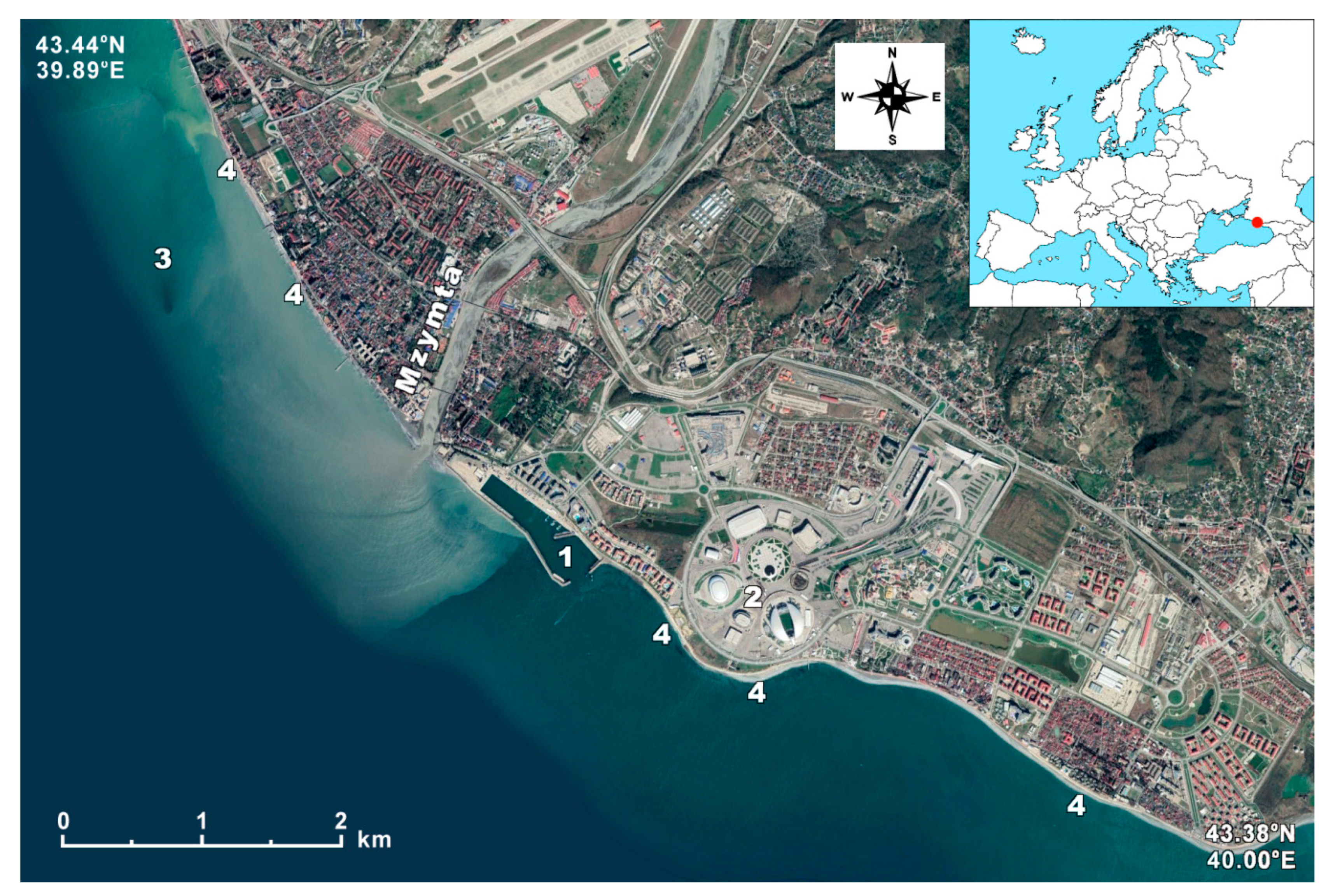
2.1. Study Area

The Mzymta River is the largest river of the Russia’s part of the Black Sea coast. It originates on the slopes of the Main Caucasus Range and has a mountainous character for most of its length. The total length of the river is 89 km and the catchment area is 885 km2 [60]. The river recharge is mixed, including precipitation, melting snow and glaciers and groundwater in the lower part. Mzymta has a high discharge in the warm season, frequent autumn floods, and a stable low water in winter.
Mzymta flow rate varies from 0.4 to 2–3 m/s. The yield of suspended sediment is directly dependent on water runoff: the greater the water discharge, the greater is the yield. The average annual amount of suspended sediment is 488,200 tons and that of bottom sediments is 141,000 tons [60]. The average annual discharge of the river is 45.6 m3/s [61].
Mzymta plume forms near the city of Adler where the river enters the Black Sea. Plume water is fresher and colder than seawater. Having a highly dynamic character, Mzymta plume is subject to a strong influence of wind and coastal system of currents [2,62], the Coriolis force, the local landscape, and stratification of the ambient sea [58]. Due to a narrow shelf zone in the southeastern Black Sea, the main element of the Black Sea circulation, the Rim Current, is often strongly pressed against the coast, at a distance of ~6 km. Therefore, being involved in the cyclonic structure of the Rim Current, Mzymta plume can spread for many kilometers along the coastline from the river mouth [63]. Interacting with sub-mesoscale and mesoscale vortex structures, the river water acts as a tracer, which aids in the studies of water exchange between the coastal zone and deep sea [64].
The infrastructure developed along the shores of Mzymta can bring a potentially significant anthropogenic impact on its waters. In the upper part of the river, there is the famous Krasnaya Polyana ski resort with a vast complex of hotels. At the mouth of the river, popular tourist attractions include extreme rafting, bungee and BASE (building, antenna, span, and earth) jumping. There are several trout farms in river bends, some of them invite tourists. The hydropower plant in Krasnaya Polyana is also located on the river and supplies electricity to the city of Sochi. The most developed is the lowland part of the river in close proximity to the coast. The cities of Sochi and Adler stretch along the seashore with numerous hotel complexes and swimming beaches. By the 2014 Winter Olympics, the eastern part of the floodplain was densely developed to build the Olympic Village, a yacht port and new artificial sandy beaches. Now, Sochi is the largest resort city in Russia, very popular throughout the year (Figure 1). Such development can dramatically contribute to pollution of the river water and, as a result, the coastal zone [65].
A possible attempt to regulate Mzymta flow into the sea and to direct it away from the yacht port in order to decrease its impact on the port protective walls can lead to destruction of the beaches just east of the port (Figure 1). Without new terrigenous material, the beaches will erode and their maintenance will be too expensive. Study, monitoring and control of this area are urgently needed to understand the changes in the coastal ecosystem due to active recreational activity and properly maintain such activity.

2.2. Data and Methods

2.2.1. Boat Measurements

Shipboard measurements were conducted from 23 April to 4 May 2019, in the estuary zone of Mzymta from a small boat called Arabella with Imereti port as point of departure. The route of Arabella within Mzymta plume consisted of 4 legs parallel to the coast, from the river mouth to a visible edge of the plume. Each sailing was organized concurrently with a satellite (Sentinel-2A/-2B MSI, Landsat-7 ETM + and Landsat-8 OLI) passage over the study area. In total, seven boat trips were completed on 23–26, 28 April and 1–2 May 2019. The summary grid of stations included more than 150 points (see Figure 2). At each station, CTD probing was performed from the surface to the bottom using a high-precision instrument RBR-Concerto of the Canadian company Richard Bransker Research Ltd. The main characteristics of the instrument are presented in Table 1. The CTD probe was equipped with a turbidity meter (TM) from Seapoint Ltd. with measurement frequency up to 6 kHz. Additionally, turbidity of the upper layer of water was measured at best possible accuracy using a portable turbidimeter (PT) TN400 from Apera Instruments. At CTD stations and in points of turbidity measurement, water sampling was performed for further evaluation of SPM.
TM is an analog sensor that detects scattered light from suspended particles in a specific volume of water placed in front of the optical window of the sensor, at a distance <5 cm. A distinctive feature of the sensor is its ability to detect light scattered from particles smaller in size than the wavelength emitted, which is 880 nm. For suspended particles whose diameters are greater than the wavelength of the light source, light scattering actually occurs through optical processes such as reflection, refraction, and diffraction [66]. A light-scattering pattern after a collision with a particle depends on the relationship between wavelength and particle size. When the particle is larger than the wavelength, light tends to scatter more intensely in the forward direction [67]. TM reports turbidity in nephelometric turbidity units (NTU). TM measuring range is from 0.05 to 15,000 NTU (±2% deviation), operating temperature 0–65 °C (temperature coefficient <0.05%/°C), depth capability 6000 m.
At the CTD stations, TM took measurements from depths of 0.35–0.50 m at best. To improve turbidity data from the upper layer of water (0.10–0.15 m), we also used PT. The instrument is equipped with an infrared light source and uses the nephelometric method that complies with ISO7207 (90° dispersion). PT measurement range is from 0 to 1000 NTU (the instrument is shipped with 4 ready-made calibration standard solutions of high-molecular polymer turbidity: 0.02 NTU, 20.0 NTU, 100 NTU, and 800 NTU), measurement accuracy varies from 0.01 to 1 NTU depending on the selected range. For each sample, two instant measurements were taken; their mean was used as a resulting value. At the same time and at the same stations, samples of water were taken from the upper surface layer for laboratory analysis.
Each optical sensor, in principle, has its own specifics. A detailed discussion can be found, for example, in [68], a work devoted to laboratory experiments on turbidity evaluation by different optical sensors.
During the boat measurements, air temperature, wind speed and wind direction were continuously recorded by the Airmar WeatherStation 150WX weather station along the course of the boat. Table 2 presents its characteristics. The display of weather station parameters was configured and realized by the factory software WeatherCaster ™ Software 3.005. Also, data on air temperature, atmospheric pressure above sea level, wind speed, wind direction and precipitation were obtained from a weather station at the airport of Sochi (https://rp5.ru/). The movement between boat stations was controlled using a chartplotter with a built-in Garmin GPSmap 541s echo sounder.

2.2.2. Laboratory Study

During the field work, 140 water samples were taken from the near-surface layer to evaluate amount and mineral composition of the suspended matter. As mentioned earlier, this was necessary in order to carry out more accurate measurements of Mzymta plume water for subsequent comparison with results derived from remote-sensing data. The volume of each sample was approximately 1.5 L. All samples were weighed in laboratory conditions with an accuracy of 0.01 g. SPM was determined gravimetrically [69,70]. Water was filtered using a vacuum unit Lafil 400-LF30 and fiberglass WHATMAN GF/F filters manufactured from hydrophobic borosilicate glass. These filters are capable to catch fine particles down to 0.7 microns. The filters were preweighed with an accuracy of 0.1 mg, and stored in a desiccator for use within 2 weeks. Water samples were filtered immediately after collection.
To remove sea salt from the suspension, filters were washed with 250 mL of distilled water after filtration. Such an amount of fresh water provided complete dissolution of the salt and its removal from the samples. The samples were stored at −20 °C until further analysis, usually within one month after sampling. Subsequently, all filtered samples were subjected to weight analysis of SPM on high-precision scales in the petrology laboratory of the Moscow State University. Suspension filters were dried for 24 h at 50 °C and reweighed. The accuracy of determining the weight of the suspended particles in the samples was ±0.0001 g. Note that suspended particulate matter includes all organic and mineral material with dimensions over approximately 0.7 mm.
The median and the interquartile range (IQR) were computed for each sample by the protocol detailed in [70]. Observations where the IQR exceeded 45% of the median SPM value were rejected.
To identify the mineral composition of the sediment, 20 samples were chosen for X-ray analysis. The samples were obtained on 26 April, 1 May and 2 May at stations located at different distances from the Mzymta mouth and covering a wide range of turbidities from minimum to maximum NTU.
X-ray scanning and analysis were performed at the Department of Oil and Gas Sedimentology and Marine Geology, College of Geology of Moscow State University. The survey was carried out on a DRON UM 1 powder diffractometer (Co Kα, λ = 1.79021 Ǻ) in the range of angles 2 Θ from 4 to 80° in continuous mode at a speed of 2° per minute. The phases were diagnosed using the MINCRYST crystallographic base for minerals and their structural analogs. The amount of the mineral phase was estimated by comparison of the intensities of the corresponding peaks.

2.2.3. Satellite Observations

All field measurements from the boat were synchronized with satellite data acquisition at best possible accuracy. The source of remote-sensing data was the instruments on board Landsat-8 and Sentinel-2 (A and B), namely, the Operational Land Imager (OLI) and Multispectral Instrument (MSI) multispectral sensors. Also, Sentinel-3 OLCI data were used to compose SPM maps. Because of their 300 m spatial resolution, no comparison with measurements at the boat stations was possible. They were used to highlight the general picture of Mzymta water distribution.
The Landsat-8 satellite, of the National Aeronautics and Space Administration (NASA) and The United States Geological Survey (USGS), is equipped with OLI and Thermal InfraRed Sensor (TIRS) multispectral scanners of medium spatial resolution in the visible and infrared ranges covering a strip about 185 km wide in a continuous mode with a flight frequency once in 7–8 days. The maximum spatial resolution of these sensors is 15, 30 and 60 m, depending on the corresponding spectral range of sensing. The paired satellites Sentinel-2A and Sentinel-2B of ESA are equipped with MSI with a spatial resolution down to 10 m. It continuously covers a strip of the surface about 290 km wide at a frequency of once every 3–10 days for the same region.
Standard algorithms for reconstructing optical parameters based on satellite data, first of all SPM and chlorophyll concentration, were initially designed for open ocean waters with a predominance of phytoplankton and its decay products, so called Case 1 type waters, whereas in our work the study region refers to Case 2 type coastal waters characterized by high turbidity and considerable influence of the coastal zone [71,72].
In the work, we used different software to process satellite data for comparison with the results of in situ measurements. First, we applied the C2RCC (Case 2 Regional Coast Colour) version of a processor originally developed by Doerffer and Schiller [37] and now implemented in the ESA Sentinel Toolbox SNAP software (https://step.esa.int/main/toolboxes/snap/). The latest development of C2RCC neural networks and the algorithm for optically complex waters are described in [43]. Although the current processor version integrates almost all the essential characteristics of the environment and the equipment applied, the algorithm developers leave open a possibility for its users to change certain input parameters and coefficients including those experimentally obtained which need permanent regional correction. They include atmosphere transmittance, reflectance parameters of a specific underlying surface, cloud risk coefficients, air pressure and other.
The recent development of more reliable technologies for the evaluation of key parameters of the marine environment has become possible due to the introduction into widespread use and accessibility of the source code of the algorithm based on the use of neural networks. The most important property of neural networks is the possibility of their training by regular updating the database of correlated input parameters and obtained characteristics of the studied medium by introducing into the model a wide range of results of real contact measurements synchronous with satellite observations in different regions and sequential refinement of the connections between neurons, that is, actually realizing multiple non-linear regression [43].
SNAP processing results that we used in our study can be presented both in a tabular form for easy comparison with in situ measurements and in the form of TCI mapping the retrieved optical characteristic with resolution close to original resolution of the satellite data. TCI do not show numerical values of the optical characteristic, but display its gradients in a way familiar to the human eye, and also carry supplementary information, such as locations of the stations, trajectory of the boat, properties of wind and currents, diurnal displacement of the plume boundary and other. For all processed satellite data, TCI were constructed at the maximum resolution (10 m).
Second, for all Landsat-8 OLI and Sentinel-2 MSI data we performed atmospheric correction with the ACOLITE DSF method. To retrieve turbidity and SPM we used two algorithms developed by a team of researchers led by Dr. Bouchra Nechad and described in detail in [31,44,45]; below they are referred to as Nechad 2009 and Nechad 2015. There were some differences in the Nechad 2009 and Nechad 2015 results, but nothing critical. In contrast, the algorithm proposed by Dogliotti et al. [32] (below referred to as Dogliotti) and intended for highly turbid waters showed rather inconsistent results.

3. Results

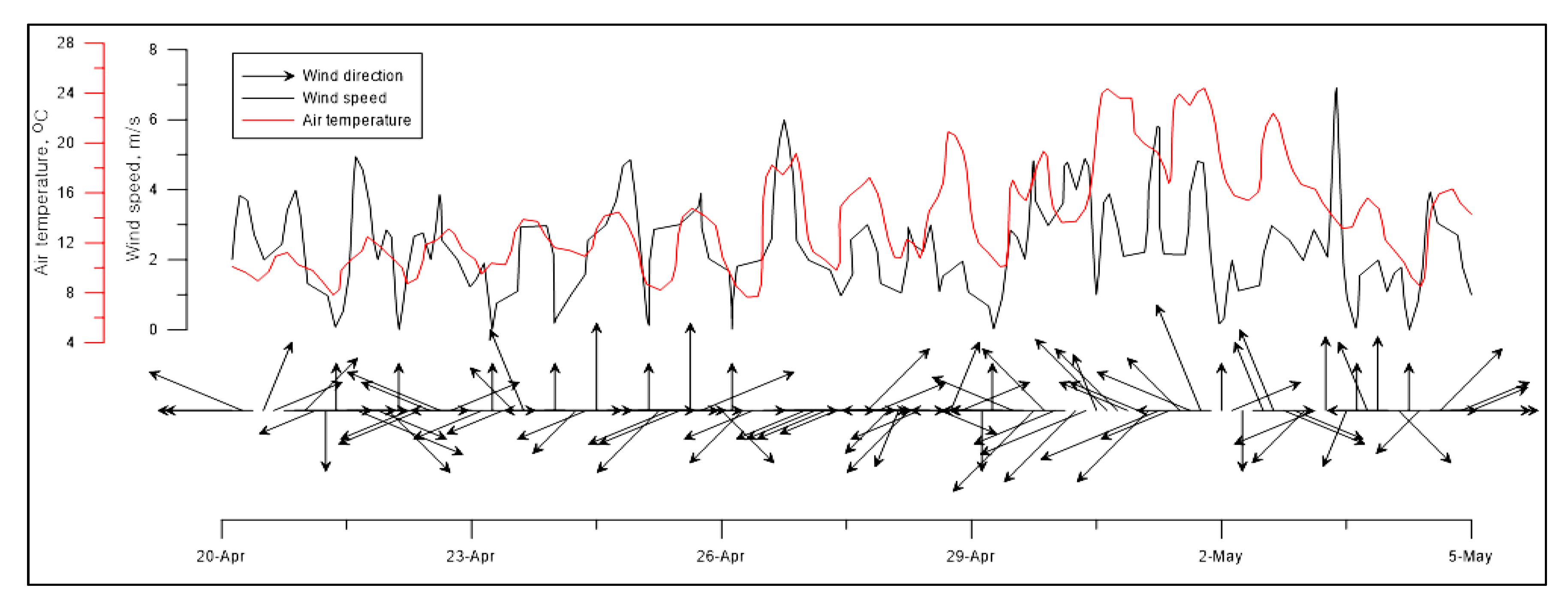
3.1. Meteorological Conditions

Knowledge of meteorological conditions is crucial for analyzing the influence of wind on the dynamics of a river plume and the influence of precipitation on the discharge and turbidity of the river. Cloud cover and air temperature affect permeability of the atmosphere, which is important for processing visible remote-sensing data.
Weather information on the days of our field work and adjacent days, from 20 April to 4 May 2019, was available from the weather station at Sochi International Airport (rp5.ru). The prevailing wind directions were: ENE—19 cases, NE—10 cases and E—11 cases in the morning; and W—22 cases in the afternoon. During NE upsurge wind, the area of the river plume reached its maximum. With E/ENE winds, the plume spread strictly westward, being pressed against the coast. In general, wind speeds were moderate and did not exceed 7 m/s. With E/ENE winds, wind speed was in the range of 2–4 m/s. Under NE winds, from 28 April to 1 May, a stronger wind was observed, from 2 to 7 m/s. With predominantly evening W winds (except on 26 April), minimum wind speed was 3 m/s and less. On 2 May and 4 May, wind directions varied. With NE winds, from 28 April to 2 May, the sky was overcast over the study area. Just before our work, on 21–23 April, slight short-term precipitation took place and on 3 May precipitation was up to 30 mm. On 26 April, the weather was cloudless over the area of observation with W winds. Air temperature ranged 8–24 °C. Its gradual increase was observed till 1–2 May. After rain on 3 May, there was a sharp decrease in air temperature to a daily average of 12–13 °C. Air temperature and wind field characteristics are presented in Figure 3.

3.2. Results of In Situ Measurements

During the field studies in April–May 2019, Mzymta plume spread strictly westward, with a sharp eastern boundary, unlike our previous observations in April 2018, when the direction of plume propagation changed depending on coastal currents [73,74].
The spreading of the plume in the western direction was caused by two factors: (1) during our work, the Rim Current jet, which is directed westward at this location, was pressed to the coast and had a high velocity of more than 0.6 m/s [63]; (2) in the eastern part the river mouth, blocks of concrete were laid to limit the spread of water in the eastern direction and to reduce the load on the structures enclosing the port facility.
Due to the relatively small size of the plume, it was possible to cover its entire area with a dense grid of measuring stations (Figure 2). At each station, measurements were taken from the surface to the bottom. For comparison with satellite observations, a special focus was on the near-surface layer.

3.2.1. Variation of Temperature, Salinity and Turbidity in the Near-Surface Layer

Temperature. During the field work, a gradual increase in water temperature in the surface layer occurred, which correlated well with a gradual increase in daily average air temperature in the region. Lowest water temperatures were typically observed close to the river mouth. At a distance of not more than 200–300 m from the mouth, the temperature in the surface layer of water, at a depth of 50–80 cm, varied in the range from 10.8 to 12.7 °C (Table 3). It gradually increased in the direction to the plume boundary with increasing mixing with seawater. The surface temperature of “proper” seawater outside the plume, varied from 12.4 to 17.3 °C. Its highest values were reached by 2 May when air warmed up to 24 °C.
Salinity. Water salinity in the surface layer at the stations closest to the mouth, varied from 6.2 to 11.4 PSU (Table 3). At the plume boundary, salinity was close to seawater, which in the Black Sea is about 18 PSU.
Turbidity. During nine expedition days, turbidity in the surface layer, according to PT measurements, soared more than eight times (Table 3), from 13 NTU in the beginning to 135 NTU in the end. The maximum turbidity was reached on 3 May, when no boat trips were conducted, after a sharp warming in the Mzymta watershed due to melting glaciers and snow in the mountains and precipitation.

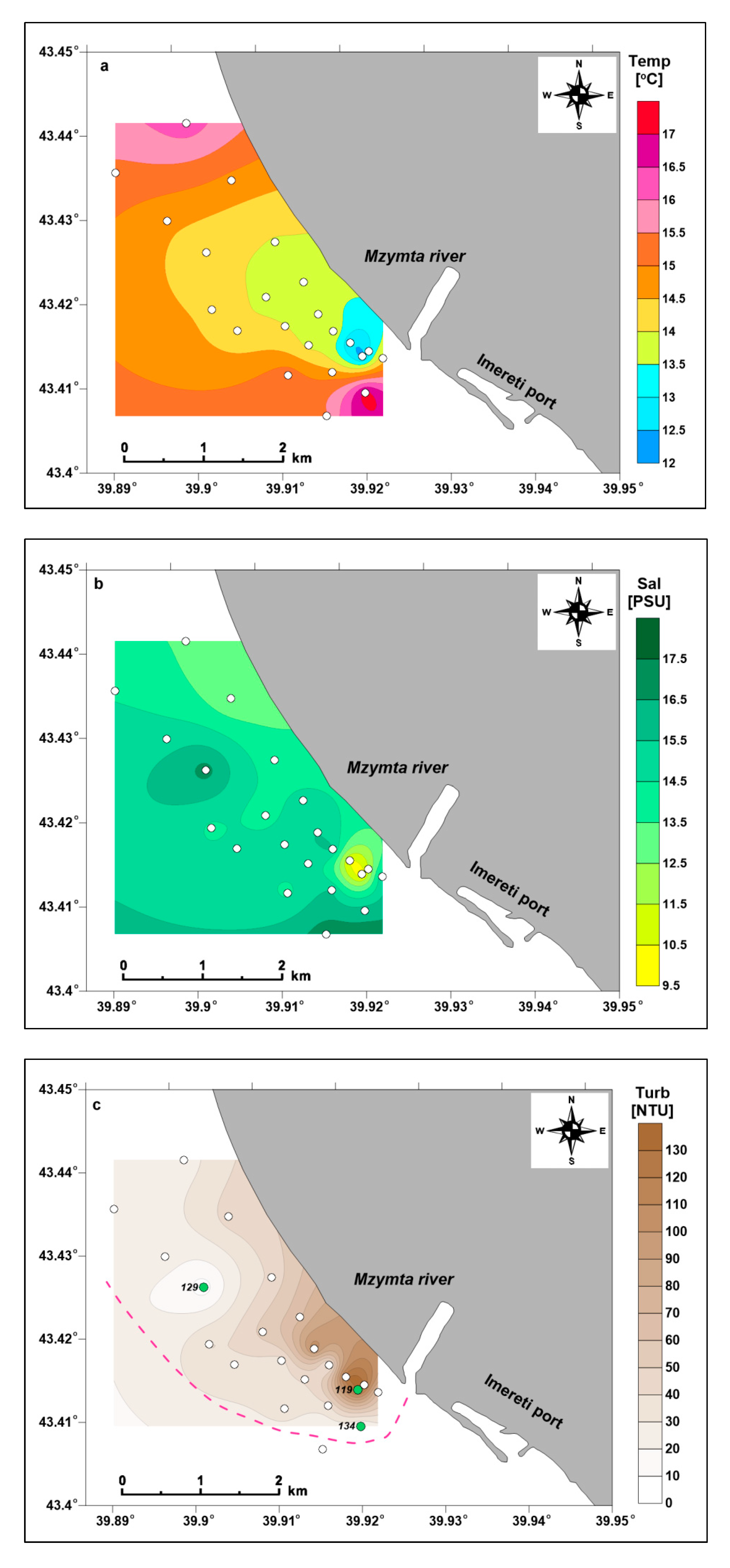
3.2.2. Spatial Distribution of Temperature, Salinity and Turbidity in the Plume

As Mzymta water spreads in the sea, changes in the basic parameters of water (temperature, salinity, turbidity) occur unevenly. This depends on speed and discharge of the river flow and on coastal currents, which are highly heterogeneous in this area [58]. As a result, local areas of increasing/decreasing turbidity and salinity are formed in the estuary zone of Mzymta. In addition, in the area of the plume there is a sewage outfall of the city of Adler that evidently influences water parameters. Figure 4 shows maps of the spatial distribution of temperature (Figure 4a), salinity (Figure 4b) and turbidity (Figure 4c) based on boat measurements using CTD and TM in the near-surface layer on 2 May 2019. In Figure 4c, pink dashed line schematically shows the boundary of the plume. Some stations on that day are also shown. They are Stations 119, 129 and 134. Station 129 is located at the outfall of the sewage pipeline. The impact of the sewage outfall is associated with a small region with almost zero turbidity and increased salinity in comparison to surrounding plume waters. This region is easily recognized in the visible satellite imagery.

3.2.3. Depth Distribution of Temperature, Salinity and Turbidity

To solve the problem of satellite data verification with the results of field measurements, it is necessary to know the depth distribution of river water parameters. The distribution of temperature and salinity over depth determines plume water stratification, which impacts the hydrodynamic processes. The thickness of the turbid water layer and turbidity depth distribution determine the depth of the water column contributing to water leaving radiance captured by the satellite sensor. Accordingly, this determines the choice of the techniques and instruments for the field measurements.
In our previous studies [73,74], we found that depth penetration of river water is small and rapidly decreases with distance from the river mouth. This was confirmed again by the observations in April and May 2019. As an example, Figure 5 shows the change in the hydrological characteristics with depth on 2 May 2019. Station 119 was located in close proximity to Mzymta mouth and Station 134 was located at the plume boundary (Figure 4c). By the conventional definition, a plume boundary is a minimum water turbidity location that is the closest to a sharp turbidity gradient. In this example (2 May), water turbidity was about 20 NTU, and outside the plume we observed values close to 0. Changes in turbidity, temperature and salinity with depth at these stations are shown in Figure 5a (Station 119) and 5b (Station 134). At Station 119, the closest to the mouth, the depth of the plume is about 2.5 m, water turbidity in the near-surface layer reaches 125 NTU, and temperature and salinity are much lower than in the underlying layer. This turbidity is the greatest for a given day. At Station 134, which is 250 m more seaward and near the border of the plume, the hydrological section looks different (Figure 5b). The thickness of river water intrusion is not more than 1 m, the turbidity of sea water is about 20 NTU, and the temperature and salinity are almost unchanged with depth.
Thus, it was determined that the depth penetration of river water sharply decreases with distance from Mzymta mouth, from 2.5 to 1 m at the plume boundary; therefore, for comparison with satellite data, all field measurements should be made in the near-surface layer. The thickness of the seasonal thermocline is about 11–12 m.

3.2.4. Results of Portable Turbidimeter (PT) Measurements in the Near-Surface Layer

After comparison of turbidity data obtained with TM and PT in the surface layer of water (see Section 4.1), it was decided to use PT measurements for further comparison with the weight method and remote sensing data, because PT is capable of taking measurements in a thinner surface layer (the first tens of centimeters) than TM.
A change in maximum water turbidity that was found with PT (most pronounced at stations located closest to the river mouth) in a thin surface layer (from 0 to 15 cm) is shown in Figure 6. During the field work, an exponential increase in this parameter was observed. The lowest value was 15.44 NTU and the highest value of 288 NTU was recorded on 4 May: a rise of 18 times in the mouth zone. Most likely, this was due to the cumulative effect of air temperature increase by the end of the field work, triggering active melting of snow and ice in the mountains, and intense (about 30 mm) precipitation on 3 May.

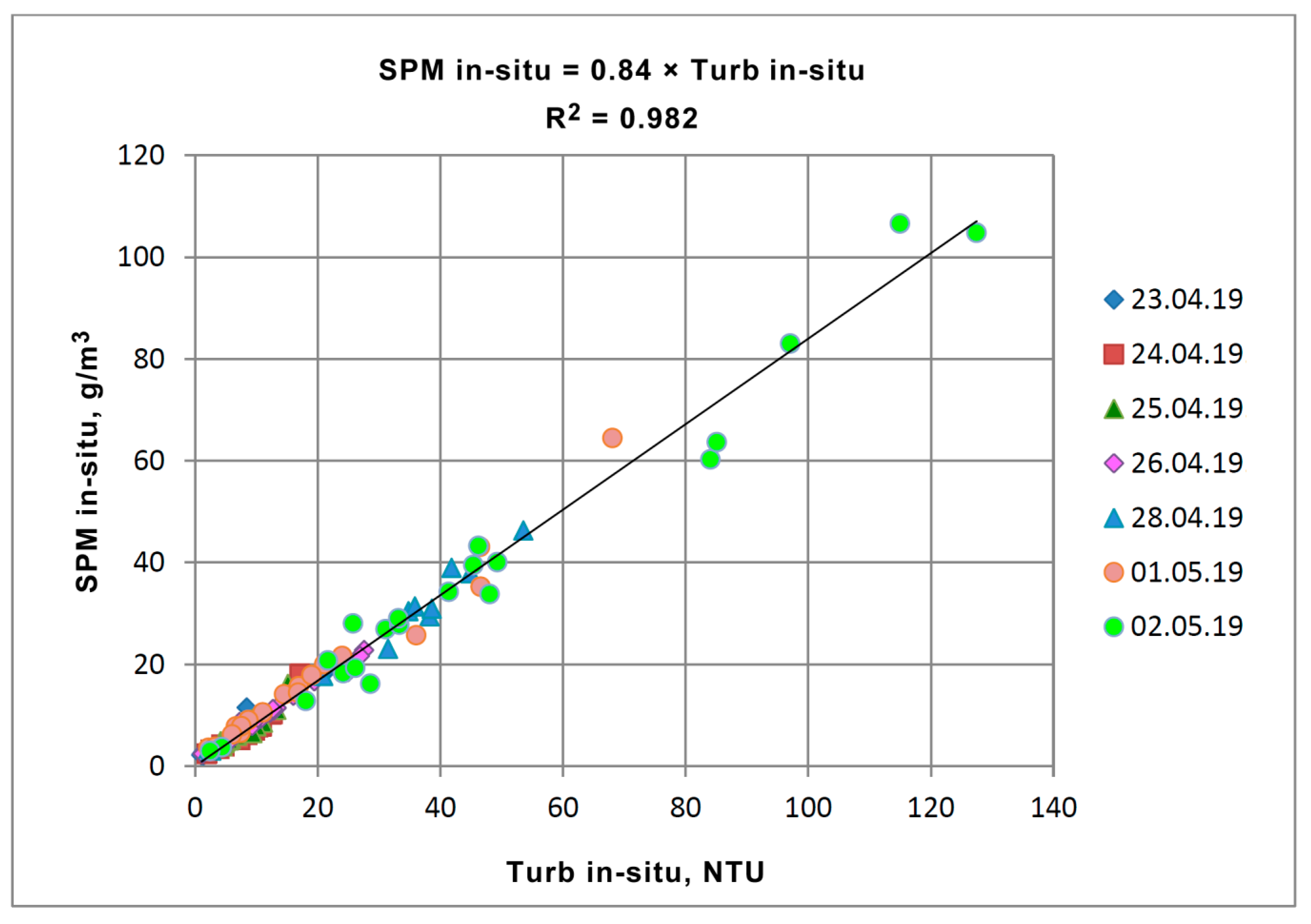
3.2.5. Correlation Analysis of Turbidity and Suspended Particulate Matter Concentration (SPM) from In Situ Measurements

During boat stations, turbidity in the plume was measured with two instruments: Apera Instruments TN400 portable turbidimeter (PT) and Seapoint turbidity meter (TM). At the same stations, water samples were collected at the same depths as PT measurements. After filtering and weighing water samples in accordance with the protocol described in [69], we obtained values of SPM hereinafter referred to as SPM in situ. Note, the water turbidity unit is NTU, while the SPM unit is g/m3, and no algorithm exists to convert one into another because the two parameters are very different in physical nature and measurement methods. Turbidity strongly depends on particle size and composition of suspended matter. One of the tasks was to define the correlation between turbidity and SPM for the study region in the period of the spring flood. The analysis shows that the SPM in situ is directly proportional to the turbidity determined with PT in the upper surface water layer (Turb in situ, NTU). As shown in Figure 7, the obtained values are well approximated by a straight line: SPM in situ = 0.84 × Turb in situ. The determination coefficient is very high: R2 = 0.982. This is typical of all water samples without exception and does not change with days of measurements or weather conditions. A similar strong relationship was determined between the SPM in situ and turbidity determined with TM, the existing differences will be addressed below in the Discussion (Section 4.1).
With such a high correlation between the PT data and the SPM in situ in this region, it seems reliable to make conversions between the turbidity and SPM units (NTU and g/m3) using the established empirical equation. The main advantage is the ability to acquire numerous data using only optical turbidity sensors without time-consuming work to determine weight turbidity. Naturally, it is necessary to conduct multiple similar experiments in different seasons and under different meteorological conditions to obtain statistically valid results.

3.2.6. Sampled SPM and Mineral Composition of Suspended Matter

The SPM in water samples collected during the field work ranged from 2 to 106 g/m3. From 23 April to 2 May, maximum SPM gradually increased from 23 g/m3 on 23–26 April; to 46 g/m3 on 28 April; 65 g/m3 on 1 May; and 106 g/m3 on 2 May. The minimum SPM values within the plume for the entire period of the study were approximately 2–3 g/m3.
X-ray phase analysis of mineral composition of the suspended matter showed that in the selected samples: (1) quartz amounted to 16–45% of the suspension mass; (2) feldspars 12–27%; (3) various clay minerals (kaolinite, montmorillonite, chlorite, hydromica, mixed layer minerals) 27–58%; (4) carbonate minerals (calcite, dolomite and aragonite) 0–22% (Table 4).

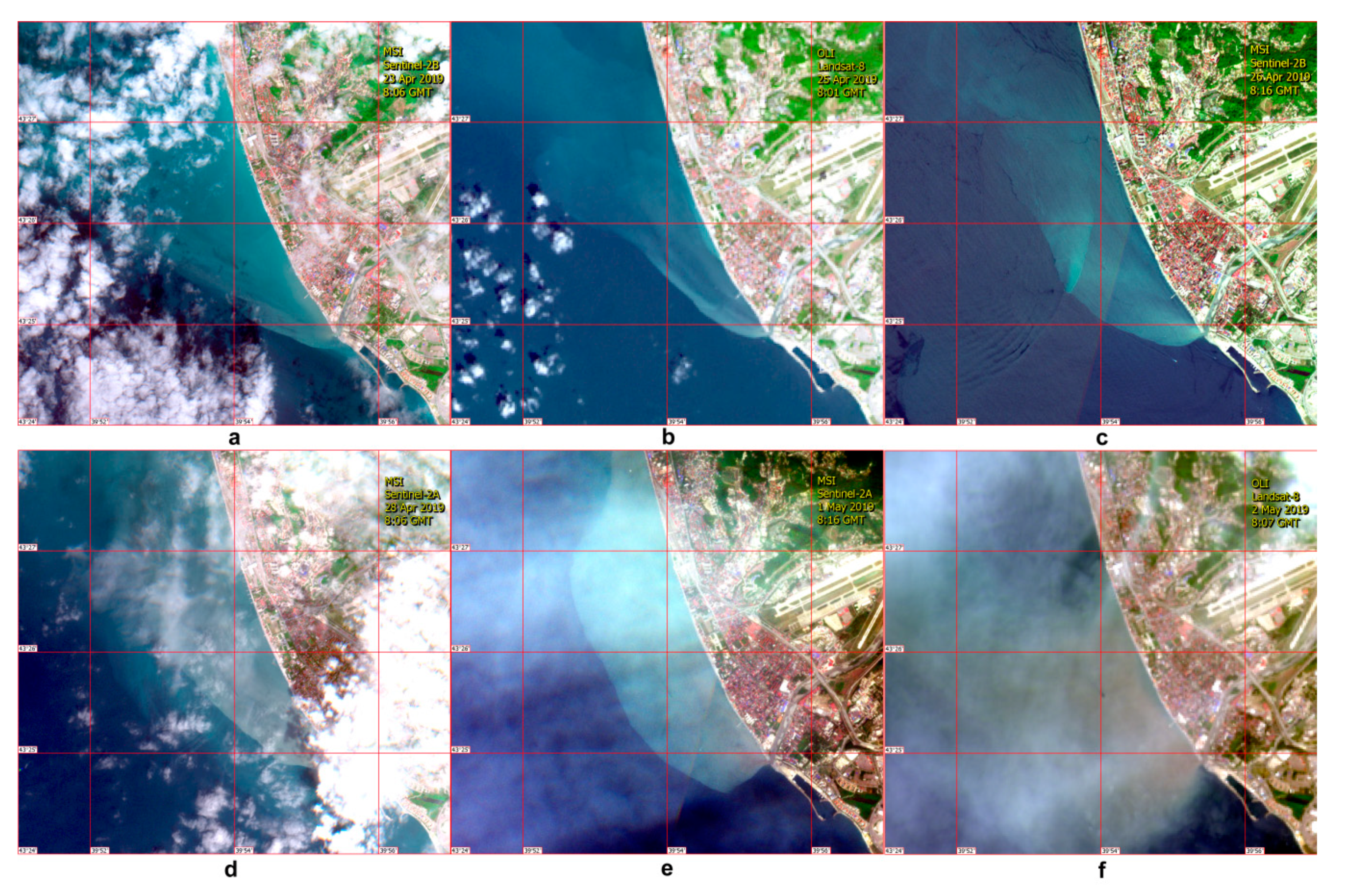
3.3. Results of Satellite Observations

3.3.1. Satellite Data Processing and Products

Field measurements were carried out concurrently with satellite remote sensing (Table 5). To efficiently compare remote sensing SPM (SPM satellite) with the in situ turbidity and sampled SPM (SPM in situ), it was necessary to use satellite optical data of a sufficiently high spatial resolution. Such data were available from Sentinel-2 MSI, with pixel resolution of 10 m in the visible range, and Landsat-8 OLI, with pixel resolution of 30 m. MSI data were obtained on 23, 26, and 28 April and on 1 May 2019; and OLI on 25 April and 2 May. On 1 and 2 May, there was haze which compromised SPM satellite data, but the plume edge was clearly visible (Figure 8). In total, during the period of field measurements, five images were acquired from Sentinel-2A/-2B MSI; one image from Landsat-7 ETM+; two images from Landsat-8 OLI/TIRS; and four images from Sentinel-3A/-3B OLCI. Based on the satellite data, TCI were composed to highlight the plume boundaries, as well as SPM satellite maps. MODIS data (Aqua/Terra) and NPP VIIRS were used as a source of auxiliary information. All satellite data were swiftly integrated into the See the Sea (STS) information system [75,76] and analyzed online to supply information for planning the next day of work (define more accurately the coordinates of hydrological stations). The satellite data and products available in the period of the field measurements are listed in Table 5.

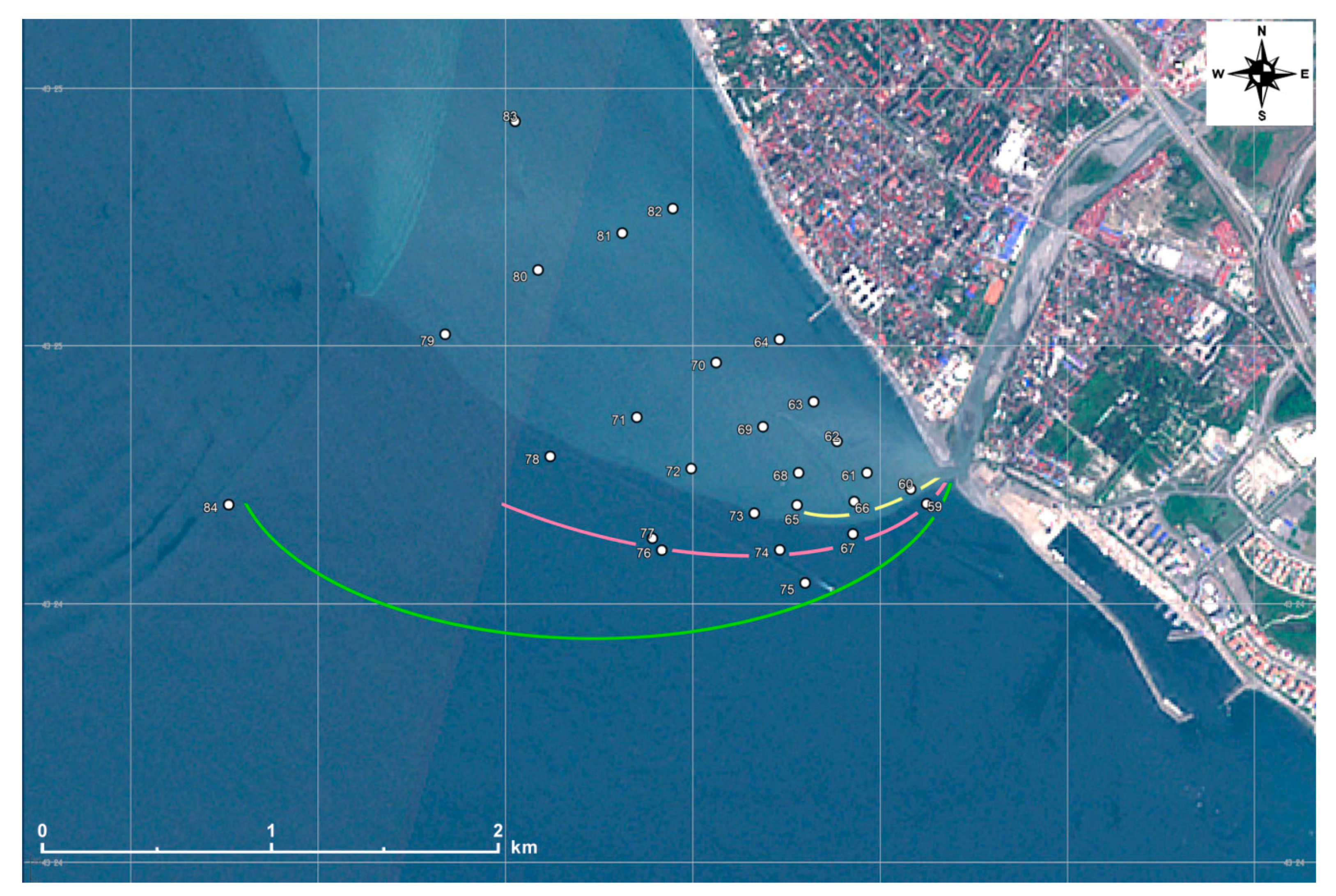
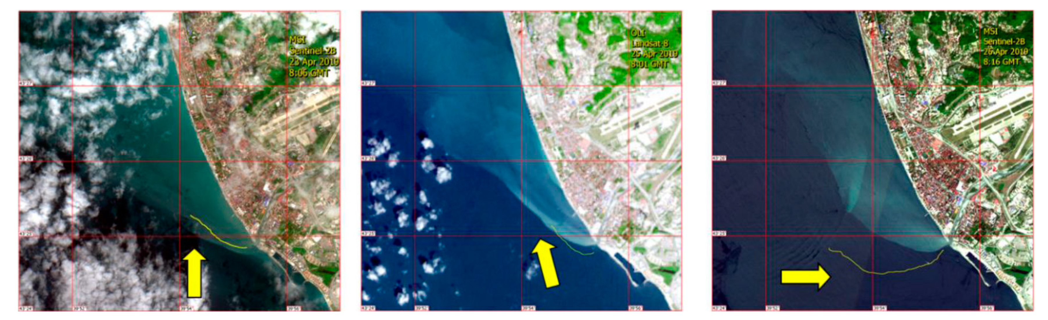
3.3.2. Plume Boundary Detection

One of the main tasks of this work was to compare SPM in situ with SPM satellite. Therefore, it was very important to carry out in situ measurements at the same time and for the same points, specifically in the region of maximum turbidity inside the plume and outside it. During boat trips, each station position was clearly defined with respect to the plume: either it was at the plume boundary, inside the plume or outside it. Each measurement cycle took about three–four hours every day to complete all hydrological stations (see Table 5). Because daily boat measurements started approximately at the time of a satellite overflight, they ended 3–4 h after it. When the measurements were completed, on its way back to port the boat followed the plume boundary visible from board, and its path was recorded using a Global Positioning System (GPS) tracker. Subsequently, the plume boundary obtained this way was plotted on the satellite image. The intermediate positions of the eastern boundary of the plume, determined from the corresponding station position records, were also plotted on the satellite image. It was found that the plume boundary changes its position at a rather high velocity, which should be taken into account when comparing the data of contact and remote measurements.
As an example, Figure 9 shows the positions of the eastern boundary of the plume on 26 April 2019, at 07:30–08:00 UTC (yellow line); 09:11–09:29 UTC (pink line) and 10:30–11:00 UTC when the boat returns to port (green line). Sentinel-2 MSI surveyed the area at 08:27 UTC. From the plume positions determined by the station locations and the plume boundary derived from the satellite image, the velocity of displacement of the plume eastern boundary was estimated to increase from 5 to 13 cm/s.

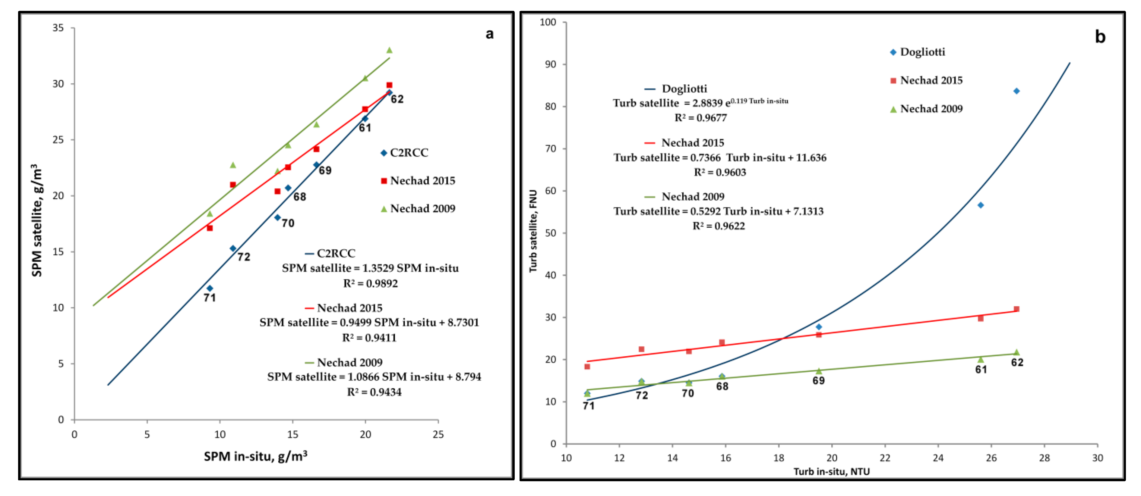
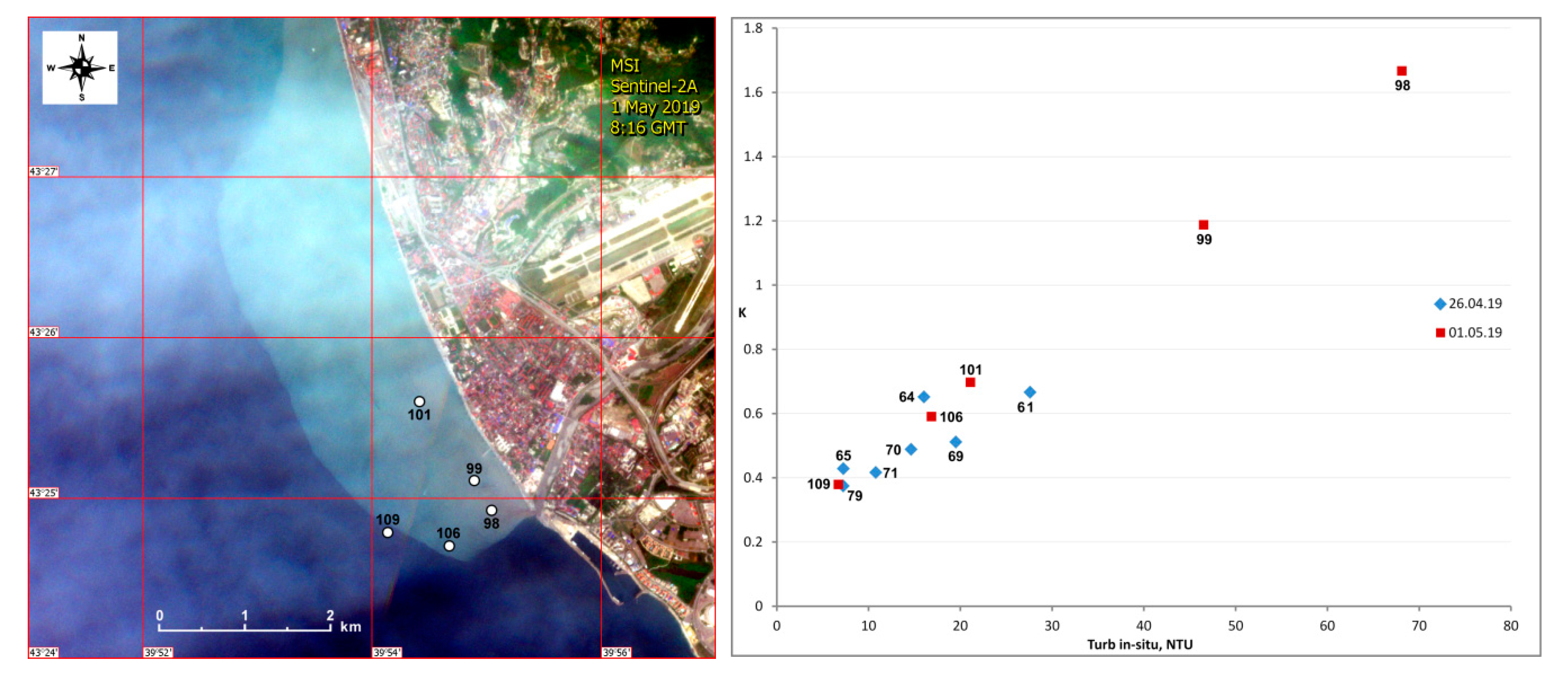
3.3.3. Correlation Analysis of SPM from Contact and Remote-Sensing Data Using Case 2 Regional Coast Color (C2RCC) Algorithm

It is difficult to expect a high correlation between SPM in situ measurements and remote sensing estimations obtained using standard algorithms. As a rule, researchers prefer to develop individual regional algorithms [21]. Nevertheless their performance depends on many factors: season, river discharge, precipitation, etc. Our aim was to compare SPM obtained from in situ measurements and SPM retrieved from satellite data using standard rather than regional algorithms. This section presents C2RCC results.
For a joint analysis of in situ and satellite data, 26 April was selected as the only cloudless day. Figure 10a presents SPM map from the Sentinel-2B MSI data. Here, the C2RCC output is total suspended matter (TSM), a term with the same meaning as SPM and similar wide use in literature. As shown in Section 3.3.2, the plume boundary was rapidly shifting towards open sea (Figure 9). Therefore, some boat stations are inside the plume identified in the satellite image, the others outside it. The MSI data were taken at 08:16 UTC. All stations can be divided into three main groups. The first group includes stations where measurements were taken at a time close to the satellite overflight. These stations were inside the plume, according to visual observations from the boat as well as satellite observations. They are Stations 61, 62, 63, 68, 69, 70, 71, 72 marked blue in Figure 10b depicting the correlation between sampled SPM in situ and SPM satellite. Station 63 failed IQR data control and was excluded from further consideration. The blue marks are approximated by a straight line SPM satellite = 1.353 × SPM in situ with reliability R2 = 0.99. Higher satellite values can be explained by the fact that each of them characterizes a certain volume of water rather than a point in the upper layer.
The second group, marked red in Figure 10b, includes Stations 65 and 66. At the time of in situ measurements they were located at the plume boundary that was quite well visible from the boat, and at the time of satellite imaging inside the plume. Therefore, SPM satellite values are much higher than SPM in situ. Special interest presents Station 60. This station was located at the mouth of the river with an SPM satellite of 51.8 g/m3. In situ measurements however gave an SPM in situ of only 10.5 g/m3. This discrepancy is most likely explained by complex conditions in close vicinity of the mouth. The river discharges water at a high speed and it vigorously interacts with seawater causing wave breaking and intense mixing. This can negatively affect both water sampling results and remote-sensing data, for instance, when the sensor captures reflection from the sea bottom in shallow waters. Also, the sample taken at this station could contain less suspended matter due to technical difficulties.
The third group of stations (73, 74, and 77) was inside the plume during water sampling (green marks). However, in situ measurements at these stations were carried out 1–1.5 h after the satellite overflight and, over this time, the plume boundary shifted by almost 250 m relative to its boundary identified in the satellite image. Therefore, in the satellite image, these stations are already outside the plume. Accordingly, at these stations the SPM satellite is lower than the SPM in situ.
Finally, as depicted in Figure 10b, Station 64 (Group 4) was located on the inner border of the plume, which was also displaced, though not as fast as the outer one. Being inside the plume during in situ measurements, Station 64 got practically outside it during satellite imagery. This explains higher values of SPM in situ than SPM satellite attributed to the station.
Thus, even using the standard C2RCC algorithm for determining SPM satellite, we achieve a good agreement with SPM in situ obtained by water sampling, but only for those stations where measurements were taken almost synchronously with satellite imaging.

3.3.4. Correlation Analysis of SPM and Turbidity from Contact and Remote-Sensing Data Using Different Algorithms

Among the main goals of our work was choosing the best standard algorithm for SPM and turbidity retrieval from remote sensing data, in terms of correlation with in situ measurements. To determine quantitative SPM, in addition to C2RCC we used Nechad 2009 [31] and Nechad 2015 [45]. SPM distribution maps built for 26 April 2019 using the three algorithms are shown in Figure 11a. Qualitatively analyzing these maps, the following conclusions can be drawn. C2RCC results look rather noisy: at low SPM, neighboring values vary significantly. The features of the plume boundary are not pronounced. The results of Nechad 2009 and Nechad 2015 are smoother and all inhomogeneities of the plume boundary can be distinguished. At the same time, the three algorithms give different distributions of the maximum SPM values in the immediate vicinity of Mzymta mouth. On the C2RCC map, the area of maximum SPM values is much larger. For processing by Nechad 2009, Nechad 2015 and comparison with C2RCC, we used only data from those stations that were performed almost synchronously with the imaging (Group 1, Figure 10b) by Sentinel-2B MSI on 26 April 2019. Figure 12a presents comparisons of SPM in situ and SPM satellite obtained by C2RCC, Nechad 2009 and Nechad 2015. No doubt, the C2RCC results best agree with the in situ data. The straight approximation line for C2RCC goes through the origin of coordinates, the determination coefficient is R2 = 0.989 (Figure 12a). For the two other algorithms, Nechad 2009 and Nechad 2015, the determination coefficients are only 0.943 and 0.941, respectively.
The main advantage of the ACOLITE algorithms is that it is possible to compare their results with in situ turbidity data, for example, measured with PT, without converting the latter to SPM in situ using the obtained dependence (Figure 7) and, more importantly, without water sampling. To quantify turbidity, we used Nechad 2009, Nechad 2015 and Dogliotti algorithms. The turbidity distribution maps compiled using these algorithms for 26 April 2019, are shown in Figure 11b. Since Nechad 2009 and Dogliotti algorithms coincide for low turbidity range, the corresponding patterns of turbidity are the same. Near Mzymta mouth, Dogliotti definitely overestimates turbidity. Interestingly, Dogliotti draws a pronounced high turbidity jet westward from the mouth zone. The existence of such a jet is confirmed, for example, by the in situ measurements at Stations 61 and 62 (Figure 10a). Although Station 62 is located somewhat farther from the mouth, but, unlike Station 61, it sits on the jet and, therefore, reports higher SPM and turbidity. A comparison of turbidities obtained by Nechad 2009, Nechad 2015 and Dogliotti (Turb satellite) with turbidity measured in situ (Turb in situ) is presented in Figure 12b. At low turbidity, less than 16 NTU (FNU), Dogliotti yields the same results as Nechad 2009. For turbidities of 20–25 NTU and higher, Dogliotti switches to another method of calculation [32] suitable for extremely turbid waters, but not for our study area (Figure 12b).
The values produced by Nechad 2009 and Nechad 2015 are well approximated by straight lines (Figure 12b). The determination coefficient is R2 = 0.96 in both cases and the lines are almost parallel. It is a puzzling fact that the lines do not go through the origin of coordinates. Obviously, further testing on a much wider array of in situ measurements is required.

4. Discussion

The data obtained by various methods during our work in April–May 2019, in the Mzymta mouth zone can be divided into two groups:
  • Data from two turbidity sensors–an optical turbidity sensor as part of the RBR-concerto CTD probe (TM) and a TN400 portable turbidimeter (PT). Both sensors provide data in NTU units and work roughly on the same principle. A significant difference is that turbidity measurements were taken at different depths, since it is impossible to obtain data in the first centimeters from the surface with the CTD probe.
  • Data on SPM at different points of the plume obtained using different methods. The first method is direct: SPM in situ was measured by weighing water samples. The second method is indirect: SPM satellite was retrieved using the standard algorithms from satellite remote sensing data.
In our work, we aimed to estimate the correlation of the data obtained from different turbidity sensors, find out if there exists a robust dependence between turbidity and SPM measured in situ, and, most importantly, reveal the correlation between satellite and contact measurements.

4.1. Performance of Contact Turbidity Sensors

As expected, turbidities obtained at the same stations with PT and TM in the near-surface horizon of 0.35–0.5 m agreed quite well. The determination coefficient of linear approximation was R2 = 0.93 and, in general, TM turbidities were slightly higher than PM ones, by a factor of 1.042. At high turbidity, a large scatter of the values is observed on both sides of the linear trend. It possibly can be explained by highly unsteady interaction of river and sea waters at the river mouth in shallow water which makes turbidity vary significantly even at close points. Moreover, clapotis and wave breaking often take place. In such conditions, it is not easy to use PT. Several measurements should be done in close points for more reliable results. Sometimes it is technically troublesome, for example, because of the risk to run aground. Meanwhile measuring with TM is much easier in such conditions, besides, each time we get at least 2 turbidity values, when TM is lowered and then raised. This was specifically observed during a sharp increase of the river discharge on May 2 when the velocity of the water flow increased from 2 m/s in the previous days to 6–8 m/s.
For turbidity values from 15 to 40 NTU, the results of measurements with different instruments almost completely coincided, with slightly higher TM values. At turbidities less than 15 NTU, an underestimation by TM can be noted. In fact, as the river waters spread into the sea, both turbidity and plume thickness sharply decrease (Figure 5a). So, the TM may eventually get below the depth of the plume penetration zone.
Considering the relationship of contact turbidity and SPM in situ, naturally, the best correlation was achieved with PT. This is easy to explain. Water samples for determining the SPM were taken at the same depth as measurements with PT, while TM measurements, as mentioned above, took place at lower points. Nevertheless, we also got a linear correlation between TM turbidity and SPM in situ, although with a slightly smaller determination coefficient as compared to PM measurements, 0.924 and 0.982, respectively. The linear relationship obtained makes it possible to convert turbidity values measured in NTU to SPM calculated in g/m3. Similar linear correlation was determined for the macrotidal estuary of the Gironde [1]. The authors of the work noted that the relationship was specific to the turbidity sensor used, but similar to those established using other instruments in other periods of time. This could be an indication that suspended matter grain size distribution and composition in the estuary did not change significantly in optical terms over the years. Such a hypothesis should be tested for Mzymta plume as well. For this purpose, one need to determine its mineral composition and establish the relationship between, for example, quartz, as the largest suspended matter constituent, and plume turbidity.
Performance of the two turbidity sensors, PT and TM, showed that, in general, it is sufficient to take measurements with only one instrument. A question arises which one suits better, in view of comparison with satellite data. To draw sound conclusions, knowledge of turbidity depth distribution is required. We believe that if river water turbidity is high and its penetration depth is small, it is more reasonable to use PT, since in this case water leaving radiance captured by the satellite sensor is formed in the near-surface horizon. If turbidity is low, water leaving radiance can be formed in a layer down to a few meters deep, so TM appears to be a more suitable instrument. In this case it is obviously necessary to obtain some integral characteristics from TM readings at various depths. This is an interesting and complex problem. As a rule, however, for comparison with satellite data, either data from various PT analogs are used [77], or data from floating spectroradiometers that are widely employed today for validating satellite data obtained during field experiments. They measure absolute spectral irradiance at the sea surface and water leaving radiance immediately under the sea surface [78]. TM data are usually used for estimating river water penetration depth and turbidity profiling.

4.2. Small-Scale River Plume Boundary Dynamics

Our work has demonstrated prime importance of tight synchronization of in situ measurements and satellite survey in the study region of Mzymta River plume. In a thematically close study [23] discussing turbidity characteristics of the Danube plume, it was noted that the maximum time gap considered between in situ SPM and high spatial resolution images acquisition was of 120 h for periods with no substantial river fluctuation and 48 h otherwise. In the case of Mzymta, the maximum time gap should not exceed 30–40 min since, as shown below, the plume boundary can move really fast. Certainly, the plume of the Danube spreads for a much greater distance from the coast, compared to Mzymta, so at considerable distances from its boundary, the plume can be regarded unchanging during a day or two. In studies conducted in the mouth regions of small rivers, such as Mzymta, one has to take into account plume spreading dynamics that is strongly influenced by wind direction [58].
After a series of experiments on 23, 25 and 26 April, small-scale displacement velocities of the plume boundary of Mzymta and their relationship with wind direction were estimated (Figure 13). The essence of the experiment was to follow the plume boundary using a GPS tracker on the way back to port after finishing the in situ measurements. It was found that with weak S/SE winds, the displacement of the plume boundary was very slow. In three hours, it shifted by 250–350 m at a velocity of 0.08–0.12 km/h under the “pressing” winds towards or along the coastal zone (23 and 25 April). The maximum displacement of the plume boundary was noted during W winds on April 26. In three hours, the boundary shifted 900 m seaward. The displacement speed was 0.3 km/h. The results of the experiments confirm the hypothesis of high mobility of the river plume as a whole and its boundary in particular. This rather complicates the comparison of quantitative remote sensing and contact data for specific stations, because during several hours of boat measurements, the internal fine structure of the plume can change significantly. Similar results are presented in [58]. Considering the impact of wind on hydrodynamic characteristics of the plume, it is possible to tentatively forecast its spreading velocity and plan more accurately the measurements at those stations whose positions relative to the plume (inside, outside, at the boundary) are not expected to change during the satellite overflight.

4.3. Performance of Satellite SPM and Turbidity Algorithms

Satellite SPM and turbidity were calculated using C2RCC, Nechad 2009, Nechad 2015 and Dogliotti algorithms. Despite its failure for turbidities greater 20 NTU in the Mzymta region, Dogliotti can be nevertheless used to reveal small scale turbidity inhomogeneities that the other two algorithms can hardly detect. The best correlation with the in situ data was achieved with C2RCC. The authors of [77] used C2RCC on Sentinel-3A OLCI L1 data using SNAP and validated the results against dedicated in situ data obtained in the Northwestern Baltic proper. Their validation campaigns took place between 2016 and 2018 in Swedish coastal waters and covered different times of year. On the basis of a large dataset, authors of [77] recommend using C2RCC, but point out the problems of atmospheric correction for pixels close to coast. The problems of adjacency effects or land contamination of satellite sea data are also discussed in [1]. Both works employ low- and medium-resolution ocean color data (MODIS and OLCI), however we do not anticipate any serious complications when using high resolution data, such as MSI and OLI, as we did in this study.
Among the atmospheric correction algorithms employed, ACOLITE DSF appears the most practical and best performing in our study region. Nechad 2009 and Nechad 2015 overestimated SPM by 1.5 times for in situ measurement range up to 15 g/m3. For the range over 20–25 g/m3, Nechad 2015 agreed well with in situ data and C2RCC results (Figure 12a). Data of 1 and 2 May, when Mzymta discharge and turbidity increased significantly, could have been of particular interest, but haze on these days did not allow obtaining meaningful satellite SPM.

4.4. Changes in the Mineral Composition of Suspended Matter Depending on Plume Water

The mineral composition of suspended matter (Table 4) shows significant variations in the content of minerals in different water samples. The quantitative ratio of mineral phases in the suspension composition depends on multiple factors.
Samples with high turbidity values, mainly from the near-mouth zones, contain a large amount of quartz. For example, samples taken on 1 May in the Mzymta estuary zone have high turbidity (up to 68 NTU) and predominance of quartz over clay minerals (see Figure 14). With the distance from the mouth, the amount of suspended matter in the water decreases and its mineral composition changes with a relative increase in clay minerals and a decrease in quartz. Samples with low turbidity values taken at the plume boundary have a significant predominance of clay minerals in the suspension.
This result is in good agreement with the well-known theory of gravitational differentiation of material, according to which a decrease in the particle size occurs with distance from the coastal zone. Clay has low hardness, is highly susceptible to mechanical weathering, and forms a fine-grained material that can be transported over long distances. Quartz is characterized by a higher hardness and has more coarse particles, which are deposited in the immediate vicinity of the river mouth.
As shown in Figure 14 right, the compositional differentiation of the suspension was most pronounced on 1 May. High turbidity values correspond to the substantially quartz composition of the suspension; at low turbidity, the suspension mainly consists of clay minerals. On 26 April, the turbidity of the plume was generally low, not more than 28 NTU. The trend of changes in the suspension composition is weakly expressed. At the moment, no unambiguous relationship has been revealed between the value of water turbidity and the mineral composition of the suspension. It is not yet possible to estimate the amount of quartz and other mineral phases in the suspension by remote sensing methods.

5. Conclusions

The paper presents the results of field studies in the northeastern part of the Black Sea in the mouth area of the Mzymta River in April and May 2019. The main objective of the study was to determine the relationships between water turbidity and SPM obtained by contact and remote sensing methods and compare performances of the C2RCC processor and the ACOLITE algorithms Nechad 2009, Nechad 2015 and Dogliotti.
It was shown that the highest correlation between the satellite and the water sampling SPM for the study area in conditions of spring flooding was achieved with C2RCC, but only for those stations where measurements were taken almost synchronously with satellite imaging. For such stations, the comparison of satellite and water sampling SPM showed a linear relationship with a reliability of 0.99. Nechad 2009, Nechad 2015 and Dogliotti overestimated SPM by 1.5 times for in situ measurement range up to 15 g/m3. For the range over 20–25 g/m3, Nechad 2015 agreed well with in situ data and C2RCC results, while Dogliotti failed.
In a highly variable environment of the Black Sea northeastern coastal zone, rapidly changing conditions often require a specific choice of both methods and instruments for collecting in situ data suitable for validating the remote-sensing algorithms. Knowledge of depth distribution of the main hydrological parameters is a key prerequisite for the right choice.
When selecting in situ measurements for comparison with satellite data, one should be particularly vigilant with respect to the high mobility of the Mzymta plume: within the 3–4 h when, as a rule, all the stations were completed, its boundary could shift considerably, either being pressed to the coast or driven away from it. The velocity of displacement of the plume boundary was estimated to increase from 5 to 13 cm/s.
A comparison of data on turbidity obtained by a portable turbidity meter and water sampling SPM shows a linear relationship with the reliability of 0.982. This relationship remained stable in time and weather conditions, which makes a portable turbidity meter a valuable tool for fast and multiple measurements. Data obtained by this method can be easily converted to SPM. This new and important result is very promising for in situ SPM evaluation in the sense that expensive and time-consuming water sampling may eventually become redundant. Moreover, without water sampling, the validation of satellite algorithms for SPM retrieval based only on portable turbidity meter data becomes a lot easier and faster: much more shorter stations can be undertaken over the same period of time and no money must be spent on processing of water samples.
Based on X-ray phase analysis of the suspended matter, changes in the total amount of quartz and clay particles were found to be a function of optical turbidity of the water samples. With a decrease in turbidity the mineral composition of the suspension changed with a relative increase in clay minerals and a decrease in quartz.
The authors hope to continue the studies to improve and validate the results presented in this paper.

Author Contributions

Conceptualization, K.N. and O.L.; methodology, K.N., Y.A., O.L. and D.S.; validation, K.N., Y.A., O.L. and Y.S.; investigation, K.N., O.L., and Y.A.; data curation, O.L. and A.S.; writing, K.N., O.L., Y.A., T.B. and Y.S.; visualization, D.S. and A.S. All authors have read and agreed to the published version of the manuscript.

Funding

Field work was funded by the Russian Foundation for Basic Research in the framework of grant No. 17-05-00715. The processing and analysis of satellite and in situ data were carried out within IKI-Monitoring Center for Collective Use using the See the Sea system, that was funded by the Ministry of Science and Higher Education of Russia, Theme “Monitoring”, State register No. 01.20.0.2.00164.

Acknowledgments

The authors are grateful to all the participants in the field work: Evgeny Krayushkin and Nikita Knyazev (Space Research Institute), Elena Zhuk (Marine Hydrophysical Institute); and Alexander Dudnikov and Egor Vlasov—the crew of the Arabella boat, from which the measurements were made. The authors are especially grateful to V.L. Kosorukov (Lomonosov Moscow State University) who carried out X-ray phase analysis of the samples. The authors would like to thank the Academic Editor and four Reviewers for their careful attitude and useful comments and suggestions.

Conflicts of Interest

The authors declare no conflict of interest.

References

  1. Doxaran, D.; Froidefond, J.-M.; Castaing, P.; Babin, M. Dynamics of the turbidity maximum zone in a macrotidal estuary (the Gironde, France): Observations from field and MODIS satellite data. Estuar. Coast. Shelf Sci. 2009, 81, 321–332. [Google Scholar] [CrossRef]
  2. Zavialov, P.O.; Makkaveev, P.N.; Konovalov, B.V.; Osadchiev, A.A.; Khlebopashev, P.V.; Pelevin, V.V.; Grabovskiy, A.B.; Izhitskiy, A.S.; Goncharenko, I.V.; Soloviev, D.M.; et al. Hydrophysical and hydrochemical characteristics of the sea areas adjacent to the estuaries of small rivers of the Russian coast of the Black Sea. Oceanology 2014, 54, 265–280. [Google Scholar] [CrossRef]
  3. Lavrova, O.Y.; Mityagina, M.I.; Kostianoy, A.G. Satellite Methods for Detecting and Monitoring Marine Zones of Ecological Risk; IKI RAN: Moscow, Russia, 2016. (In Russian) [Google Scholar]
  4. Garvine, R.W. A steady state model for buoyant surface plume hydrodynamics in coastal waters. Tellus 1982, 34, 293–306. [Google Scholar] [CrossRef] [Green Version]
  5. Garvine, R.W.; Monk, J.D. Frontal structure of a river plume. J. Geophys. Res. 1974, 79, 2251–2259. [Google Scholar] [CrossRef]
  6. Lavrova, O.Y.; Soloviev, D.M.; Strochkov, M.A.; Bocharova, T.Y.; Kashnitsky, A.V. River plumes investigation using Sentinel-2A MSI and Landsat-8 OLI data. In SPIE Remote Sensing, Proceedings of the Remote Sensing of the Ocean, Sea Ice, Coastal Waters, and Large Water Regions 2016, Edinburgh, UK, 26–29 September 2016; SPIE—International Society for Optics and Photonics: Bellingham, WA, USA, 2016; Volume 9999, p. 99990G. [Google Scholar] [CrossRef]
  7. Zajączkowski, M.; Darecki, M.; Szczuciński, W. Report on the development of the Vistula river plume in the coastal waters of the Gulf of Gdansk during the May 2010 flood. Oceanologia 2010, 52, 311–317. [Google Scholar] [CrossRef] [Green Version]
  8. Abascal-Zorrilla, N.; Vantrepotte, V.; Huybrechts, N.; Ngoc, D.D.; Anthony, E.J.; Gardel, A. Dynamics of the Estuarine Turbidity Maximum Zone from Landsat-8 Data: The Case of the Maroni River Estuary, French Guiana. Remote Sens. 2020, 12, 2173. [Google Scholar] [CrossRef]
  9. Doxaran, D.; Froidefond, J.M.; Castaing, P. A reflectance band ratio used to estimate suspended matter concentrations in sediment-dominated coastal waters. Int. J. Remote Sens. 2002, 23, 5079–5085. [Google Scholar] [CrossRef]
  10. Babin, M.A.; Morel, V.; Fournier-Sicre, F.F.; Stramski, D. Light scattering properties of marine particles in coastal and open ocean waters as related to the particle mass concentration. Limnol. Oceanogr. 2003, 48, 843–859. [Google Scholar] [CrossRef]
  11. Constantin, S.; Doxaran, D.; Constantinescu, S. Estimation of water turbidity and analysis of its spatio-temporal variability in the Danube River plume (Black Sea) using MODIS satellite data. Cont. Shelf Res. 2016, 112, 14–30. [Google Scholar] [CrossRef]
  12. Chen, J.; D’Sa, E.; Cui, T.; Zhang, X. A semi-analytical total suspended sediment retrieval model in turbid coastal waters: A case study in Changjiang River Estuary. Opt. Express 2013, 21, 13018–13031. [Google Scholar] [CrossRef]
  13. Gernez, P.; Lafon, V.; Lerouxel, A.; Curti, C.; Lubac, B.; Cerisier, S.; Barillé, L. Toward Sentinel-2 High Resolution Remote Sensing of Suspended Particulate Matter in Very Turbid Waters: SPOT4 (Take5) Experiment in the Loire and Gironde Estuaries. Remote Sens. 2015, 7, 9507–9528. [Google Scholar] [CrossRef] [Green Version]
  14. Ou, S.; Zhang, H.; Wang, D. Dynamics of the buoyant plume off the Pearl River estuary in summer. Environ. Fluid Mech. 2009, 9, 471–492. [Google Scholar] [CrossRef] [Green Version]
  15. Petus, C.; Chust, G.; Gohin, F.; Doxaran, D.; Froidefond, J.M.; Sagarminaga, Y. Estimating turbidity and total suspended matter in the Adour River plume (South Bay of Biscay) using MODIS 250-m imagery. Cont. Shelf Res. 2010, 30, 379–392. [Google Scholar] [CrossRef] [Green Version]
  16. Devlin, M.J.; Petus, C.; da Silva, E.; Tracey, D.; Wolff, N.H.; Waterhouse, J.; Brodie, J. Water Quality and River Plume Monitoring in the Great Barrier Reef: An Overview of Methods Based on Ocean Colour Satellite Data. Remote Sens. 2015, 7, 12909–12941. [Google Scholar] [CrossRef] [Green Version]
  17. Ody, A.; Doxaran, D.; Vanhellemont, Q.; Nechad, B.; Novoa, S.; Many, G.; Bourrin, F.; Verney, R.; Pairaud, I.; Gentili, B. Potential of High Spatial and Temporal Ocean Color Satellite Data to Study the Dynamics of Suspended Particles in a Micro-Tidal River Plume. Remote Sens. 2016, 8, 245. [Google Scholar] [CrossRef] [Green Version]
  18. Ouillon, S.; Forget, P.; Froidefond, J.-M.; Naudin, J.-J. Estimating suspended matter concentrations from SPOT data and from field measurements in the Rhone River plume. Marine Technology Society. Mar. Technol. Soc. J. 1997, 31, 15. [Google Scholar]
  19. Berdeal, I.; Hickey, B.; Kawase, M. Influence of wind stress and ambient flow on high discharge river plume. J. Geophys. Res. 2002, 107, 3130. [Google Scholar] [CrossRef]
  20. Pruszak, Z.; van Ninh, P.; Szmytkiewicz, M.; Ostrowski, R. Hydrology and morphology of two river mouth regions (temperate Vistula Delta and subtropical Red River Delta). Oceanologia 2005, 47, 365–385. [Google Scholar]
  21. Kopelevich, O.; Sheberstov, S.; Burenkov, V.; Vazyulya, S.; Likhacheva, M. Assessment of underwater irradiance and absorption of solar radiation at water column from satellite data. In SPIE Remote Sensing, Proceedings of the Current Research on Remote Sensing, Laser Probing, and Imagery in Natural Waters, Moscow, Russian, 1–3 January 2007; SPIE—International Society for Optics and Photonics: Bellingham, WA, USA, 2007; Volume 6615, p. 661507. [Google Scholar] [CrossRef]
  22. Mulligan, R.P.; Perrie, W.; Solomon, S. Dynamics of the Mackenzie River plume on the inner Beaufort shelf during an open water period in summer. Estuar. Coast. Shelf Sci. 2010, 89, 214–220. [Google Scholar] [CrossRef]
  23. Güttler, F.N.; Niculescu, S.; Gohin, F. Turbidity retrieval and monitoring of Danube Delta waters using multi-sensor optical remote sensing data: An integrated view from the delta plain lakes to the western–northwestern Black Sea coastal zone. Remote Sens. Environ. 2013, 132, 86–101. [Google Scholar] [CrossRef] [Green Version]
  24. Lavrova, O.Y.; Soloviev, D.M.; Mityagina, M.I.; Strochkov, A.Y.; Bocharova, T.Y. Revealing the influence of various factors on concentration and spatial distribution of suspended matter based on remote sensing data. In SPIE Remote Sensing, Proceedings of the Remote Sensing of the Ocean, Sea Ice, Coastal Waters, and Large Water Regions 2015, Toulouse, France, 21–24 September 2015; SPIE—International Society for Optics and Photonics: Bellingham, WA, USA, 2015; Volume 9638, p. 96380D. [Google Scholar] [CrossRef]
  25. Cai, L.; Tang, D.; Li, X.; Zheng, H.; Shao, W. Remote sensing of spatial-temporal distribution of suspended sediment and analysis of related environmental factors in Hangzhou Bay, China. Remote Sens. Lett. 2015, 6, 597–603. [Google Scholar] [CrossRef]
  26. Osadchiev, A.A. Estimation of river discharge based on remote sensing of a river plume. In SPIE Remote Sensing, Proceedings of the Remote Sensing of the Ocean, Sea Ice, Coastal Waters, and Large Water Regions 2015, Toulouse, France, 21–24 September 2015; SPIE—International Society for Optics and Photonics: Bellingham, WA, USA, 2015; Volume 9638, p. 96380H. [Google Scholar] [CrossRef]
  27. Warrick, J.A.; DiGiacomo, P.M.; Weisberg, S.B.; Nezlin, N.P.; Mengel, M.; Jones, B.H.; Ohlmann, J.C.; Washburn, L.; Terrill, E.J.; Farnsworth, K.L. River plume patterns and dynamics within the Southern California Bight. Cont. Shelf Res. 2007, 27, 2427–2448. [Google Scholar] [CrossRef]
  28. Many, G.; Bourrin, F.; De Madron, X.D.; Pairaud, I.; Gangloff, A.; Doxaran, D.; Ody, A.; Verney, R.; Menniti, C.; Le Berre, D.; et al. Particle assemblage characterization in the Phone River ROFI. J. Mar. Syst. 2016, 157, 39–51. [Google Scholar] [CrossRef] [Green Version]
  29. Novoa, S.; Doxaran, D.; Ody, A.; Vanhellemont, Q.; Lafon, V.; Lubac, B. Atmospheric corrections and multi-conditional algorithm for multi-sensor remote sensing of suspended particulate matter in low-to-high turbidity levels Coastal Waters. Remote Sens. 2017, 9, 61. [Google Scholar] [CrossRef] [Green Version]
  30. Gohin, F. Annual cycles of chlorophyll-a, non-algal suspended particulate matter, and turbidity observed from space and in-situ in coastal waters. Ocean Sci. 2011, 7, 705–732. [Google Scholar] [CrossRef] [Green Version]
  31. Nechad, B.; Ruddick, K.G.; Park, Y. Calibration and validation of a generic multisensor algorithm for mapping of total suspended matter in turbid waters. Remote Sens. Environ. 2010, 114, 854–866. [Google Scholar] [CrossRef]
  32. Dogliotti, A.I.; Ruddick, K.G.; Nechad, B.; Doxaran, D.; Knaeps, E. A single algorithm to retrieve turbidity from remotely-sensed data in all coastal and estuarine waters. Remote Sens. Environ. 2015, 156, 157–168. [Google Scholar] [CrossRef] [Green Version]
  33. Vantrepotte, V.; Loisel, H.; Mériaux, X.; Neukermans, G.; Dessailly, D.; Jamet, C.; Gensac, E.; Gardel, A. Seasonal and inter-annual (2002-2010) variability of the suspended particulate matter as retrieved from satellite ocean color sensor over the French Guiana coastal waters. J. Coast. Res. 2011, 64, 1750–1754. [Google Scholar]
  34. Tavora, J.; Boss, E.; Doxaran, D.; Hill, P. An Algorithm to Estimate Suspended Particulate Matter Concentrations and Associated Uncertainties from Remote Sensing Reflectance in Coastal Environments. Remote Sens. 2020, 12, 2172. [Google Scholar] [CrossRef]
  35. Knaeps, E.; Ruddick, K.G.; Doxaran, D.; Dogliotti, A.I.; Nechad, B.; Raymaekers, D.; Sterckx, S. A SWIR based algorithm to retrieve total suspended matter in extremely turbid waters. Remote Sens. Environ. 2015, 168, 66–79. [Google Scholar] [CrossRef] [Green Version]
  36. Han, B.; Loisel, H.; Vantrepotte, V.; Mériaux, X.; Bryère, P.; Ouillon, S.; Dessailly, D.; Xing, Q.; Zhu, J. Development of a Semi-Analytical Algorithm for the Retrieval of Suspended Particulate Matter from Remote Sensing over Clear to Very Turbid Waters. Remote Sens. 2016, 8, 211. [Google Scholar] [CrossRef] [Green Version]
  37. Doerffer, R.; Schiller, H. The MERIS Case 2 water algorithm. Int. J. Remote Sens. 2007, 28, 517–535. [Google Scholar] [CrossRef]
  38. Schroeder, T.; Schaale, M.; Fischer, J. Retrieval of atmospheric and oceanic properties from MERIS measurements: A new Case-2 water processor for BEAM. Int. J. Remote Sens. 2007, 28, 5627–5632. [Google Scholar] [CrossRef]
  39. Gangloff, A.; Verney, R.; Doxaran, D.; Ody, A.; Estournel, C. Investigating Rhône River plume (Gulf of Lions, France) dynamics using metrics analysis from the MERIS 300m Ocean Color archive (2002–2012). Cont. Shelf Res. 2007, 144, 98–111. [Google Scholar] [CrossRef] [Green Version]
  40. Xue, K.; Ma, R.; Shen, M.; Li, Y.; Duan, H.; Cao, Z.; Wang, D.; Xiong, J. Variations of suspended particulate concentration and composition in Chinese lakes observed from Sentinel-3A OLCI images. Sci. Total Environ. 2020, 721, 137774. [Google Scholar] [CrossRef]
  41. Gower, J.; Doerffer, R.; Borstad, G.A. Interpretation of the 685 nm peak in water-leaving radiance spectra in terms of fluorescence, absorption and scattering, and its observation by MERIS. Int. J. Remote Sens. 1999, 20, 1771–1786. [Google Scholar] [CrossRef]
  42. Gower, J.; King, S.; Borstad, G.A.; Brown, L. Detection of intense plankton blooms using the 709 nm band of the MERIS imaging spectrometer. Int. J. Remote Sens. 2005, 26, 2005–2012. [Google Scholar] [CrossRef]
  43. Brockmann, C.; Doerffer, R.; Peters, M.; Kerstin, S.; Embacher, S.; Ruescas, A. Evolution of the C2RCC Neural Network for Sentinel 2 and 3 for the Retrieval of Ocean Colour Products in Normal and Extreme Optically Complex Waters. In Living Planet Symposium, Proceedings of the ESA Living Planet Symposium, Prague, Czech Republic, 9–13 May 2016; ESA-SP: São Paulo, Brazil, 2016; Volume 740, ISBN 978-92-9221-305-3. [Google Scholar]
  44. Nechad, B.; Ruddick, K.G.; Neukermans, G. Calibration and validation of a generic multisensor algorithm for mapping of turbidity in coastal waters. In SPIE Remote Sensing, Proceedings of the Remote Sensing of the Ocean, Sea Ice, Coastal Waters, and Large Water Regions 2009, Berlin, Germany, 31 August–3 September 2009; SPIE—International Society for Optics and Photonics: Bellingham, WA, USA, 2009; Volume 7473, p. 74730H. [Google Scholar] [CrossRef]
  45. Nechad, B.; Ruddick, K.; Schroeder, T.; Oubelkheir, K.; Blondeau-Patissier, D.; Cherukuru, N.; Brando, V.; Dekker, A.; Clementson, L.; Banks, A.C.; et al. CoastColour Round Robin data sets: A database to evaluate the performance of algorithms for the retrieval of water quality parameters in coastal waters. Earth Syst. Sci. Data 2015, 7, 319–348. [Google Scholar] [CrossRef] [Green Version]
  46. Martins, V.S.; Barbosa, C.C.F.; De Carvalho, L.A.S.; Jorge, D.S.F.; Lobo, F.D.L.; Novo, E.M.L.M. Assessment of Atmospheric Correction Methods for Sentinel-2 MSI Images Applied to Amazon Floodplain Lakes. Remote Sens. 2017, 9, 322. [Google Scholar] [CrossRef] [Green Version]
  47. Warren, M.A.; Simis, S.G.H.; Martinez-Vicente, V.; Poser, K.; Bresciani, M.; Alikas, K.; Spyrakos, E.; Giardino, C.; Ansper, A. Assessment of atmospheric correction algorithms for the Sentinel-2A MultiSpectral Imager over coastal and inland waters. Remote Sens. Environ. 2019, 225, 267–289. [Google Scholar] [CrossRef]
  48. Caballero, I.; Stumpf, R.P. Atmospheric correction for satellite-derived bathymetry in the Caribbean waters: From a single image to multi-temporal approaches using Sentinel-2A/B. Opt. Express 2020, 28, 11742–11766. [Google Scholar] [CrossRef] [PubMed]
  49. Gernez, P.; Doxaran, D.; Barillé, L. Shellfish Aquaculture from Space: Potential of Sentinel2 to Monitor Tide-Driven Changes in Turbidity, Chlorophyll Concentration and Oyster Physiological Response at the Scale of an Oyster Farm. Front. Mar. Sci. 2017, 4, 137. [Google Scholar] [CrossRef] [Green Version]
  50. Vanhellemont, Q. Adaptation of the dark spectrum fitting atmospheric correction for aquatic applications of the Landsat and Sentinel-2 archives. Remote Sens. Environ. 2019, 225, 175–192. [Google Scholar] [CrossRef]
  51. Vanhellemont, Q.; Ruddick, K. Turbid wakes associated with offshore wind turbines observed with Landsat 8. Remote Sens. Environ. 2014, 145, 105–115. [Google Scholar] [CrossRef] [Green Version]
  52. Vanhellemont, Q.; Ruddick, K. Advantages of high quality SWIR bands for ocean colour processing: Examples from Landsat-8. Remote Sens. Environ. 2015, 161, 89–106. [Google Scholar] [CrossRef] [Green Version]
  53. Vanhellemont, Q.; Ruddick, K. ACOLITE for Sentinel-2: Aquatic Applications of MSI imagery. In Living Planet Symposium, Proceedings of the ESA Living Planet Symposium, Prague, Czech Republic, 9–13 May 2016; ESA-SP: São Paulo, Brazil, 2016; Volume 740. [Google Scholar]
  54. Vanhellemont, Q.; Ruddick, K. Atmospheric correction of metre-scale optical satellite data for inland and coastal water applications. Remote Sens. Environ. 2018, 216, 586–597. [Google Scholar] [CrossRef]
  55. Ilori, C.O.; Pahlevan, N.; Knudby, A. Analyzing Performances of Different Atmospheric Correction Techniques for Landsat 8: Application for Coastal Remote Sensing. Remote Sens. 2019, 11, 469. [Google Scholar] [CrossRef] [Green Version]
  56. Bernardo, N.; Watanabe, F.; Rodrigues, T.; Alcântara, E. Atmospheric correction issues for retrieving total suspended matter concentrations in inland waters using OLI/Landsat-8 image. Adv. Space Res. 2017, 59, 2335–2348. [Google Scholar] [CrossRef] [Green Version]
  57. Korotkina, O.A.; Zavialov, P.O.; Osadchiev, A.A. Submesoscale variability of the current and wind fields in the coastal region of Sochi. Oceanology 2011, 51, 745–754. [Google Scholar] [CrossRef]
  58. Osadchiev, A.; Sedakov, R. Spreading dynamics of small river plumes off the northeastern coast of the Black Sea observed by Landsat 8 and Sentinel-2. Remote Sens. Environ. 2019, 221, 522–533. [Google Scholar] [CrossRef]
  59. Lebedev, S.A.; Kostianoy, A.G.; Soloviev, D.M.; Kostianaia, E.A.; Ekba, Y.A. On a relationship between the river runoff and the river plume area in the northeastern Black Sea. Int. J. Remote Sens. 2020, 41, 5806–5818. [Google Scholar] [CrossRef]
  60. Dzhaoshvili, S. Rivers of the Black Sea; Technical Report # 71; European Environment Agency: Copenhagen, Denmark, 2010. [Google Scholar]
  61. Drozhzhina, K.V. Features of the climatic conditions of the Mzymta river basin for recreational activities. Young Sci. 2013, 5, 196–198. [Google Scholar]
  62. Zavialov, P.O.; Barbanova, E.S.; Pelevin, V.V. Estimating the deposition of river-borne suspended matter from the joint analysis of suspension concentration and salinity. Oceanology 2015, 55, 832–836. [Google Scholar] [CrossRef]
  63. Lavrova, O.Y.; Soloviev, D.M.; Strochkov, A.Y.; Nazirova, K.R.; Krayushkin, E.V.; Zhuk, E.V. The use of mini-drifters in coastal current measurements conducted concurrently with satellite imaging. Issl. Zemli Kosmosa 2019, 5, 36–49. [Google Scholar] [CrossRef]
  64. Aibulatov, N.A.; Zavialov, P.O.; Pelevin, V.V. Peculiarities of hydrophysical self-purification of Russian coastal zone of the Black Sea near the river estuaries. Geoekologiya 2008, 4, 301–310. [Google Scholar]
  65. Nazirova, K.; Lavrova, O.; Mityagina, M.; Krayushkin, E. Influence of vortex structures on the spread of pollution. In Proceedings of the 12th International Conference on the Mediterranean Coastal Environment, Medcoast 2015, Varna, Bulgaria, 6–10 October 2015; pp. 985–996. [Google Scholar]
  66. van de Hulst, H.C. Light Scattering by Small Particles; Dover Publications: New York, NY, USA, 1981. [Google Scholar]
  67. Sadar, M. Turbidity Science. Technical Information Series. 1998, Booklet 11. Available online: https://www.hach.com/asset-get.download-en.jsa?code=61792 (accessed on 2 November 2020).
  68. Merten, G.H.; Capel, P.D.; Minella, J.P.G. Effects of suspended sediment concentration and grain size on three optical turbidity sensors. J. Soils Sediments 2014, 14, 1235–1241. [Google Scholar] [CrossRef]
  69. Van Der Linde, D.W. Protocol for determination of total suspended matter in oceans and coastal zones. JRC Tech. Note I 1998, 98, 182. [Google Scholar]
  70. Neukermans, G.; Loisel, H.; Meriaux, X.; Astoreca, R.; McKee, D. In situ variability of mass-specific beam attenuation and backscattering of marine particles with respect to particle size, density, and composition. Limnol. Oceanogr. 2012, 57, 124–144. [Google Scholar] [CrossRef] [Green Version]
  71. Morel, A.; Prieur, L. Analysis of variations in ocean color. Limnol. Oceanogr. 1977, 22, 709–722. [Google Scholar] [CrossRef]
  72. Mobley, C.D.; Stramski, D.; Bissett, W.P.; Boss, E. Optical Modeling of Ocean Waters: Is the Case 1–Case 2 Classification Still Useful? Oceanography 2004, 17, 60–67. [Google Scholar] [CrossRef]
  73. Nazirova, K.; Lavrova, O.; Krayushkin, E. Features of monitoring near the mouth zones by contact and contactless methods. In SPIE Remote Sensing, Proceedings of the Remote Sensing of the Ocean, Sea Ice, Coastal Waters, and Large Water Regions 2019, Strasbourg, France, 9–12 September 2019; SPIE—International Society for Optics and Photonics: Bellingham, WA, USA, 2019; Volume 11150, p. 111500H. [Google Scholar] [CrossRef]
  74. Nazirova, K.R.; Lavrova, O.Y.; Krayushkin, E.V.; Soloviev, D.M.; Zhuk, E.V.; Alferyeva, Y.O. Identification features of river plume parameters by in-situ and satellite methods. Sovr. Probl. DZZ Kosm. 2019, 16, 227–243. [Google Scholar] [CrossRef]
  75. Mityagina, M.I.; Lavrova, O.Y.; Uvarov, I.A. See the Sea: Multi-user information system for investigating processes and phenomena in coastal zones via satellite remotely sensed data, particularly hyperspectral data. In SPIE Remote Sensing, Proceedings of the Remote Sensing of the Ocean, Sea Ice, Coastal Waters, and Large Water Regions 2014, Amsterdam, The Netherlands, 22–25 September 2014; SPIE—International Society for Optics and Photonics: Bellingham, WA, USA, 2014; Volume 9240, p. 92401C. [Google Scholar] [CrossRef]
  76. Lavrova, O.Y.; Mityagina, M.I.; Uvarov, I.A.; Loupian, E.A. Current capabilities and experience of using the See the Sea information system for studying and monitoring phenomena and processes on the sea surface. Sovr. Probl. DZZ Kosm. 2019, 16, 266–287. [Google Scholar] [CrossRef]
  77. Kyryliuk, D.; Kratzer, S. Evaluation of Sentinel-3A OLCI Products Derived Using the Case-2 Regional CoastColour Processor over the Baltic Sea. Sensors 2019, 19, 3609. [Google Scholar] [CrossRef] [Green Version]
  78. Glukhovets, D.; Kopelevich, O.; Yushmanova, A.; Vazyulya, S.; Sheberstov, S.; Karalli, P.; Sahling, I. Evaluation of the CDOM Absorption Coefficient in the Arctic Seas Based on Sentinel-3 OLCI Data. Remote Sens. 2020, 12, 3210. [Google Scholar] [CrossRef]
Figure 1. Study area in the northeastern part of the Black Sea. 1 Imereti port; 2 Olympic Park; 3 wastewater outfall; 4 beaches.
Remotesensing 13 00143 g001
Figure 2. Map of 2019 hydrological stations.
Remotesensing 13 00143 g002
Figure 3. Meteorological conditions during 2019 in situ measurements (rp5.ru).
Remotesensing 13 00143 g003
Figure 4. Maps of spatial distribution on 2 May 2019: (a) water temperature; (b) salinity; (c) turbidity from CTD and TM measurements. Pink dashed line indicates the boundary of the river plume.
Remotesensing 13 00143 g004
Figure 5. Typical CTD + TM casts: (a) Station 119—the closest to the mouth; (b) Station 134—near plume boundary (see Figure 4). Red line—temperature, green line—salinity, black line—turbidity.
Remotesensing 13 00143 g005
Figure 6. Changes in PT maximum turbidity (black line), daily average air temperature (dashed line) and precipitation (blue columns).
Remotesensing 13 00143 g006
Figure 7. Comparison of SPM in the water samples (SPM in situ) and turbidity determined with PT (Turb in situ) for all measurement days in April–May 2020.
Remotesensing 13 00143 g007
Figure 8. Fragments of satellite images obtained during the measurement period: 23 April 2019, Sentinel-2B Multispectral Instrument (MSI) (a); 25 April 2019, Landsat-8 Operational Land Imager (OLI) (b); 26 April 2019, Sentinel-2B MSI (c); 28 April 2019, Sentinel-2A MSI (d); 1 May 2019, Sentinel-2A MSI (e); 2 May 2019, Landsat-8 OLI (f).
Remotesensing 13 00143 g008
Figure 9. Plume boundary positions on 26 April 2019, at 07:30–08:00 UTC (yellow line); 09:11–09:29 UTC (pink line) and 10:30–11:00 UTC (green line) superimposed on a Sentinel-2B MSI image taken at 08:27 UTC on the same day.
Remotesensing 13 00143 g009
Figure 10. Case 2 Regional Coast Color (C2RCC) performance on Sentinel-2B MSI data of 26 April 2019: (a) SPM map with positions of the measurement stations; (b) quantitative comparison of SPM satellite and water sampling SPM in situ. In Panel (b), Group 1 stations (blue) retained their positions relative to the plume boundary during the time between satellite overflight and water sampling; Group 2 (red) stations were located directly at the plume boundary at the time of water sampling. In the satellite image, they are inside the plume; Group 3 (green) stations were inside the plume at the time of water sampling. In the satellite image, they are outside the plume; Group 4 station (magenta) is located opposite the pier. The station numbers are indicated beside the marks. The trend line is drawn only for Group 1.
Remotesensing 13 00143 g010
Figure 11. Performance of different satellite algorithms to map: (a) SPM; (b) turbidity, retrieved from Sentinel-2B MSI data of 26 April 2019.
Remotesensing 13 00143 g011
Figure 12. Performance of different satellite retrieval algorithms compared with in situ measurements: (a) SPM satellite vs. SPM in situ; (b) satellite turbidity (Turb satellite) vs. in situ turbidity obtained with PT (Turb in situ). The station numbers are indicated beside the marks.
Remotesensing 13 00143 g012
Figure 13. River plume boundary at the time of satellite overflight in the images of 23, 25 and 26 April 2019 (true color images (TCI)). In the images, yellow line is a GPS track along the boundary of the plume 3 h after the satellite overflight. Yellow arrow indicates prevailing wind direction.
Remotesensing 13 00143 g013
Figure 14. Left: fragment of a Sentinel-2A MSI satellite image of May 1. Marks indicate locations where samples were taken for X-ray phase analysis. Right: graph shows the ratio of the percentage of quartz in the dry matter of the suspension to the percentage of clay minerals (K) depending on turbidity (Turb in situ, NTU). The station numbers are indicated beside the marks. Positions of the stations on 26 April (blue marks) are shown in Figure 10a.
Remotesensing 13 00143 g014
Table 1. The main characteristics of RBR-Concerto CTD instrument.
ParameterRangeInitial
Accuracy
ResolutionTime
Constant
Typical Stability/
Per Year
Max.
Depth (m)
Sampling Speed
(Hz)
Conductivity0–85 mS */cm±0.003 mS/cm0.001 mS/cm~1 s0.010 mS/cm2002–6
Temperature−5 °C to 35 °C±0.002°0.00005 °C~1 s0.002 °C2002–6
Depth0–200 m±0.05% FS ** 0.001% FS<0.01 s0.1% FS2002–6
*—millisiemens. **—full scale.
Table 2. The main characteristics of Airmar WeatherStation 150WX.
ParameterRangeAccuracyResolution
wind speed0–40 m/s5%/10 m/s0.1 m/s
wind direction0° to 359.9°±3°/10 m/s0.1°
air temperature−40 °C to 80 °C±1.1 °C/20 °C0.1 °C
barometric pressure300 to 1100 hPa±0.5 hPa0.1 hPa
pinch and roll50°±1° in range of ±30°0.1°
Table 3. Maximum and minimum values of temperature, salinity, turbidity and suspended particulate matter concentration (SPM) in the surface water layer on days of boat measurements.
DateMin
Temperature, °C
Max
Temperature, °C
Min Salinity, PSUMax Turbidity, NTUMax SPM, g/m3
PT *TM **Water Sample
23 April 201911.0412.3711.36223118.7
24 April 201911.6113.6510.95131618.1
25 April 201911.1713.2410.38152016.1
26 April 201910.7713.536.23283122.8
28 April 201911.0914.466.55547846.3
1 May 201912.6915.509.24687564.5
2 May 201912.2817.259.80125129106.6
* measured with TN400 portable turbidimeter, Apera Instruments. ** measured with Turbidity Meter, Seapoint Ltd.
Table 4. Turbidity in the upper near-surface layer, sampled SPM and mineral composition of suspension.
DateStationPT Water Turbidity, NTUSampled SPM, g/m3Quartz, mas.% *Feldspars mas.% *Clay Minerals, mas.% *Carbonate Minerals, mas.% *K **
26 April60_12822.828214290.67
26 April641613.830244600.65
26 April6577.3192345100.43
26 April692016.6232145100.51
26 April701514.022244590.49
26 April71119.3162338220.42
26 April7978.617244590.38
01 May986864.545202781.67
01 May994743.138243261.19
01 May1012120.031194460.70
01 May1061714.427194660.59
01 May10977.822125880.38
02 May1209783.035164540.78
02 May1254833.830155140.60
02 May1282619.424274260.58
02 May1334134.330145140.58
02 May1373327.828194760.60
* percentage of total weight of the suspended matter. ** K—ratio of the mass of quartz to the mass of clay minerals in suspension.
Table 5. Satellite information available during field measurements.
DateTime UTCSensorSatellitePixel Resolution, mProductBoat Measurements, Time UTC
23 April08:17MSISentinel-2B10TCI, SPM7:42–10:38
24 April07:59ETM+Landsat-730TCI7:33–11:41
25 April08:01OLI/TIRSLandsat-830/60TCI, SST, SPM, CHL7:37–11:08
07:56OLCISentinel-3B300SPM
26 April07:30OLCISentinel-3B300SPM7:27–10:32
08:27MSISentinel-2B10TCI, SPM
10:12VIIRSNPP1000SST, WLR, CHL
28 April08:17MSISentinel-2A10TCI (cloud)7:37–9:17
30 April07:26OLCISentinel-3B300SPMNo measurements at stations
01 May08:27MSISentinel-2A10TCI (cloud)7:35–10:56
02 May 08:07OLI/TIRSLandsat-830TCI (cloud)7:30–11:07
04 May 08:02OLCISentinel-3A300SPMNo measurements at stations
Publisher’s Note: MDPI stays neutral with regard to jurisdictional claims in published maps and institutional affiliations.

