Prediction of Maize Yield at the City Level in China Using Multi-Source Data


1
Key Laboratory of Regional Ecology and Environmental Change, School of Geography and Information Engineering, China University of Geosciences, Wuhan 430074, China
2
Hubei Key Laboratory of Critical Zone Evolution, School of Geography and Information Engineering, China University of Geosciences, Wuhan 430074, China
3
School of Electronic Information, Wuhan University, Wuhan 430079, China
*
Author to whom correspondence should be addressed.
Remote Sens. 2021, 13(1), 146; https://0-doi-org.brum.beds.ac.uk/10.3390/rs13010146
Submission received: 27 November 2020
/
Revised: 25 December 2020
/
Accepted: 3 January 2021
/
Published: 5 January 2021
Abstract
:Maize is a widely grown crop in China, and the relationships between agroclimatic parameters and maize yield are complicated, hence, accurate and timely yield prediction is challenging. Here, climate, satellite data, and meteorological indices were integrated to predict maize yield at the city-level in China from 2000 to 2015 using four machine learning approaches, e.g., cubist, random forest (RF), extreme gradient boosting (Xgboost), and support vector machine (SVM). The climate variables included the diffuse flux of photosynthetic active radiation (PDf), the diffuse flux of shortwave radiation (SDf), the direct flux of shortwave radiation (SDr), minimum temperature (Tmn), potential evapotranspiration (Pet), vapor pressure deficit (Vpd), vapor pressure (Vap), and wet day frequency (Wet). Satellite data, including the enhanced vegetation index (EVI), normalized difference vegetation index (NDVI), and adjusted vegetation index (SAVI) from the Moderate Resolution Imaging Spectroradiometer (MODIS), were used. Meteorological indices, including growing degree day (GDD), extreme degree day (EDD), and the Standardized Precipitation Evapotranspiration Index (SPEI), were used. The results showed that integrating all climate, satellite data, and meteorological indices could achieve the highest accuracy. The highest estimated correlation coefficient (R) values for the cubist, RF, SVM, and Xgboost methods were 0.828, 0.806, 0.742, and 0.758, respectively. The climate, satellite data, or meteorological indices inputs from all growth stages were essential for maize yield prediction, especially in late growth stages. R improved by about 0.126, 0.117, and 0.143 by adding climate data from the early, peak, and late-period to satellite data and meteorological indices from all stages via the four machine learning algorithms, respectively. R increased by 0.016, 0.016, and 0.017 when adding satellite data from the early, peak, and late stages to climate data and meteorological indices from all stages, respectively. R increased by 0.003, 0.032, and 0.042 when adding meteorological indices from the early, peak, and late stages to climate and satellite data from all stages, respectively. The analysis found that the spatial divergences were large and the R value in Northwest region reached 0.942, 0.904, 0.934, and 0.850 for the Cubist, RF, SVM, and Xgboost, respectively. This study highlights the advantages of using climate, satellite data, and meteorological indices for large-scale maize yield estimation with machine learning algorithms.

1. Introduction
The global demand for the use of agricultural crops as food, feed, and bioenergy will continue to grow in the coming decades [1]. Accurate and timely estimation of yield can help make informed policies and investments in agriculture and increase market stability and efficiency [2,3]. Maize is an important cereal crop and is cultivated almost everywhere around the world. The relationships between agroclimatic input parameters and maize are complicated and building a fundamental explanatory model that integrates all of these factors has become extremely challenging and difficult [4]. To solve this problem, a variety of methods mainly based on crop growth models and empirical models have been constructed in relevant studies to predict crop yield [5].
Crop growth models, which are widely used in crop yield forecasting, can accurately simulate crop yield at the field scale by explaining the relationships of crop growth with soil, cultivation management, atmospheric, or other factors [6,7,8,9]. Statistical models, which construct a statistical relationship between crop influence factors and yields, are major tools in estimating crop yield [10]. Compared with crop growth models, the statistical models have the characteristics of fewer inputs required, simplicity, and relatively high predictive skill when enough training data are available [11]. Statistical models have also been widely used in crop yield estimation [12,13,14]. Combined with official data, this method showed its usefulness for crop monitoring. However, empirical models also have shortcomings, such as collinearity between predictors due to sampling extrapolation problems [15,16,17]. Along with advances in technology, a number of machine learning approaches have been proposed to predict yield across a large number of crops and a broad geographic swath [18,19,20,21]. Machine learning can acquire useful information and uncover hidden features from a variety of training data, which could potentially bring better predictions than traditional statistical approaches [11].
Crop yield forecasting systems can be classified into four types based on the data used: surveys, remote sensing, climate data, and combined climate-remote sensing [13]. Climate change is essential for crop growth [10,22]. Martinez et al. [23] used climate indices to predict maize yield and evaluated the impact of large-scale oceanic and atmospheric climate patterns on maize yield in the southeast United States during the period 1970–2005. They found that climate and technologies were the main factors that determined annual national coconut production. Moreover, an increasing number of studies have attempted to use remote sensing data for crop prediction [24,25,26,27]. Satellite data have been recognized as a useful tool for yield estimation owing to their repetitive and timely synoptic coverage [28]. Additionally, satellite data has the probability of improving yield prediction by deriving spatially explicit crop information in progress. Specifically, the enhanced vegetation index (EVI) and the normalized difference vegetation index (NDVI) have been recognized for their value in monitoring crop conditions and predicting crop yield since the early 1980s [17,29]. The NDVI was highly correlated with canopy background variations; however, it had some limitations related to soil background brightness and saturation problems with high biomass values [30]. Conversely, the soil adjusted vegetation index (SAVI) could minimize the soil brightness problem that exists in the NDVI [31]. Hence, all three vegetation indices were important in tracking the phenological events and monitoring seasonal variations in crops. Moreover, the final yield was related to green biomass during the head-filling period, according to Son et al. [31]; thus, the saturation problem of the NDVI would lead to inaccuracy. This problem could be solved by using the EVI, which was proposed to reduce atmospheric influences and decouple the canopy background signal, according to Deng et al. [32] and Son et al. [31]. Currently, studies have been conducted using the SAVI by taking the influence of the soil background in the early period and the interference of high vegetation coverage in the late period into consideration [33,34,35]. Guo et al. [34] incorporated temporal remote sensing vegetation indices (VIs) and the wheat grow-PROSAIL model-simulated VIs to forecast regional crop yields in Yanhu Farm and Baimahu Farm. Their results showed that the SAVI, with a root mean square error (RMSE) of 510.68 kg/ha, was superior to other VIs when used as the assimilating parameter. Remote sensing data are often incorporated with climate data to obtain a synergistic overview of yield prediction accuracy [1]. Many studies have attempted to use meteorological indices in maize yield prediction. For example, Pede et al. [36] assessed the potential benefits of LST derived by satellite for maize yield prediction across the US Corn Belt from 2010 to 2016 by using metrics of killing degree day (KDD) and growing degree day (GDD). Feng et al. [37] developed a hybrid yield forecasting approach by combing climate extremes, NDVI, crop-process model simulated biomass, and the Standardized Precipitation Evapotranspiration Index (SPEI) with a regression model (RF or multiple linear regression (MLR)). They found that the forecasting system based on RF was better than that based on MLR at each forecasting event.
In China, many studies have attempted to estimate crop yield [38,39,40], however, most researches were based on a single model for small-scale yield forecasting. Few studies used agrometeorological indicators such as GDD, EDD, and SPEI for yield forecasting; thus, it is necessary to explore the possibility of multiple models to predict crop yield in China using multi-source data.
All climate, satellite data, and meteorological indices have had some success in yield predictions by applying machine learning methods [20,29,36], however, previous studies about crop yield prediction still had some limitations. First, these studies paid more attention to machine learning methods such as RF and SVM. In contrast, the newest studies [1,41,42] confirmed that novel machine learning methods, such as cubist and extreme gradient boosting (Xgboost), had the advantage of improving the accuracy of estimating R. Second, satellite data such as the EVI and NDVI have been widely used in yield predictions. Still, few studies have considered the SAVI to be superior to these indices [34]. Third, these studies usually conducted their experiments at a large-scale, such as the provincial or state level [10,43], and few studies have focused on crop yield forecasting at the city level [13]. Moreover, maize is one of the major cereal crops grown around the world, providing the primary caloric and nutritional source for millions of people worldwide. Accurate and rapid monitoring and prediction of maize growth is essential to ensure food security. Hence, executing a reliable, large-scale prediction of maize yield using climate and satellite data at the city level is needed.
Here, this study combined climate, satellite data, and meteorological indices to forecast maize yield using four machine learning methods in China. This study was designed to address the following objectives: (1) to evaluate the prediction accuracies of the four machine learning algorithms by comparing seven forms of input data and discuss the highest estimating correlation coefficient (R) of maize yield prediction; (2) to explore the contributions of climate, satellite data and meteorological indices to maize yield prediction and analyze the divergence in climate and satellite data in different growth stages from maize yield prediction; and (3) to investigate the divergences in R of maize yield prediction between five maize-growing regions.
2. Materials and Methods
2.1. Study Area
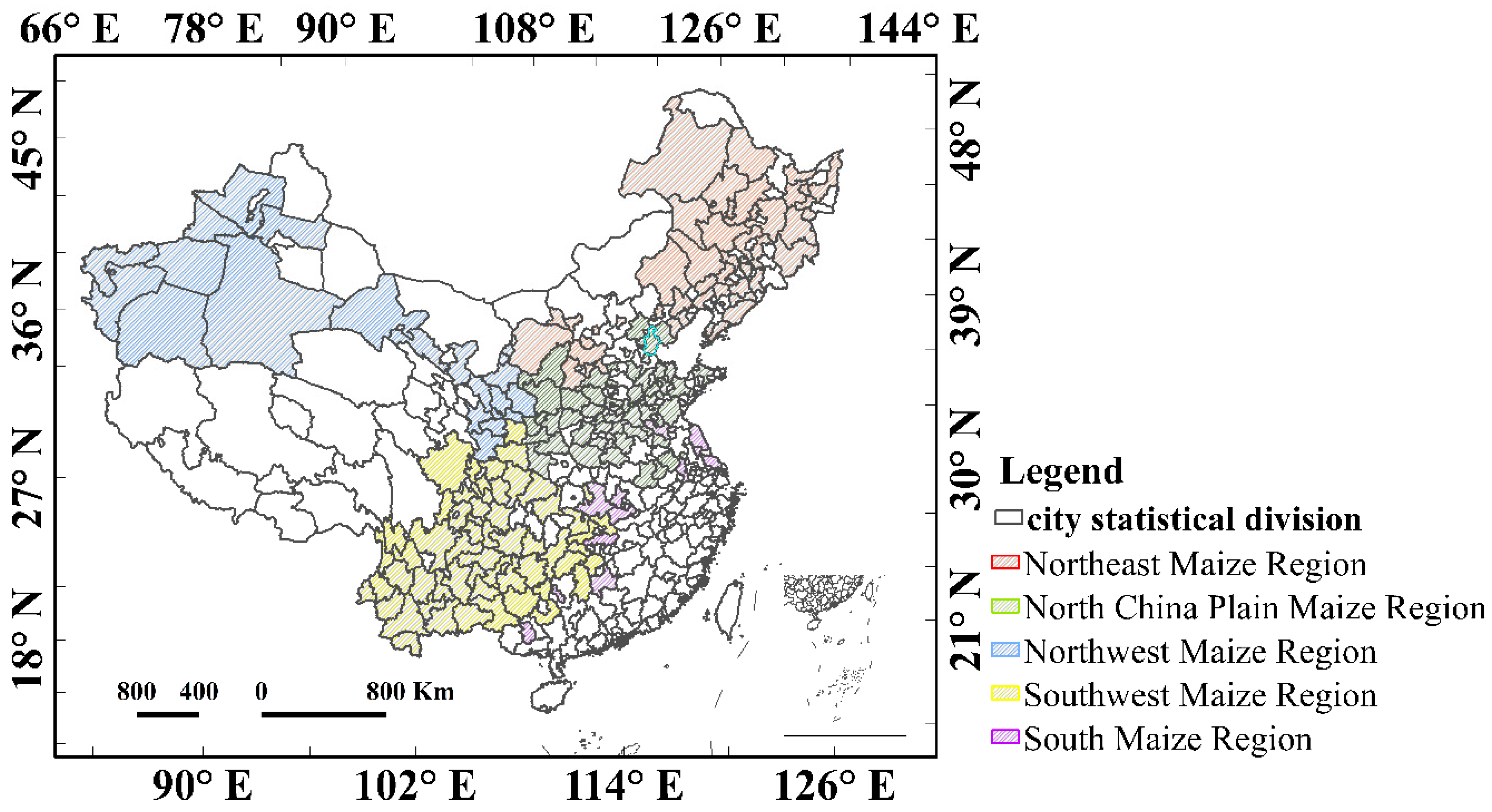
The total land area of China is approximately 9.6 million km2; specifically, mountains, plateaus, and hills account for approximately 67% of the land area, and basins and plains account for approximately 33% of the land area, with high elevation in the western part and low elevation in the eastern part. In terms of climate type, the eastern part of China has a monsoon climate (which can also be divided into subtropical monsoon climates), the northwest part has a subordinate temperate continental climate, and the Qinghai–Tibet Plateau has an alpine climate. China is one of the main producers and exporters of maize globally, accounting for 21.5% of global maize cropping area and 22.8% of global maize production [44], and it plays a major role in the global market. This study covers maize production in 213 cities, whereas nine cities are missing from 2000 to 2015, mainly in five maize-growing regions of China, which includes Northeast China, North China Plain, Northwest China, Southwest China, and South China (Figure 1). The detailed information of five regions during the maize growing season is shown in Table 1.
2.2. Materials
Here, the growing season of maize in China was defined from March to August, and the analysis focused on this period. Five types of data, city-level maize statistics, maize cropping region masks, climate data, satellite data, and meteorological indices, were used in this study.
2.2.1. Crop Yield
The city-level maize yields used in this study were survey data collected by the National Bureau of Statistics of China from 2000 to 2015. Due to the limited yield records, 203 cities were selected. The maize cropping regions were derived from the International Food Policy Research Institute (IFPRI) spatial production allocation model (SPAM) (2000, 2005, and 2010) beta cropland product, which was generated in collaboration with the International Institute for Applied Systems Analysis (IIASA). The SPAM [45] was on the basis of the IIASA best available cropland mask, subnation-level statistics, and a series of suitability variables [3]. These features estimated cropland distribution within five arc-minute grids by using a cross-entropy approach to 0.0833 degrees.
2.2.2. Climate, Satellite Data, and Meteorological Indices
Eight variables, including maximum temperature (Tmx), mean temperature (Tmp), minimum temperature (Tmn), potential evapotranspiration (Pet), vapor pressure (Vap), precipitation (Pre), cloud cover percentage (Cld), and wet day frequency (Wet), were collected from the Climatic Research Unit (CRU) [46] at 1-month intervals and at a 0.5 degree spatial resolution. The vapor pressure deficit (Vpd) was calculated using the method described in Cai et al. [29]. In addition, the four radiation-related variables used in this study were the diffuse flux of shortwave radiation (SDf), the direct flux of shortwave radiation (SDr), the diffuse flux of photosynthetic active radiation (PDf), and the direct flux of photosynthetic active radiation (PDr), which were developed by the satellite sensor of the Clouds and the Earth’s Radiant Energy System (CERES). It was provided as a monthly product with a resolution of 1 degree.
Satellite data were derived from the Moderate Resolution Imaging Spectroradiometer (MODIS, collection 6), including the MOD13A3 EVI and the NDVI, with a 1 km spatial resolution and monthly temporal resolution. The SAVI was calculated using the bands from the MOD13A3 product [34].
Meteorological indices included the GDD, EDD, and SPEI. Daily maximum and minimum temperature from 2000 to 2015 were obtained from the climate data-sharing service system of the China Meteorological Administration (CMA) with a spatial resolution of 0.5 degrees (http://data.cma.cn). The GDD and EDD, which were a representation of effective thermal units and extreme heat events, respectively, were computed as following according to previous studies [47,48].
where Tmax and Tmin are maximum and minimum temperature (°C), respectively.
The SPEI product covering the period between 2000 and 2015 was obtained from the Spanish National Research Council (CSIC), with a monthly time resolution and a 0.5 degrees spatial resolution. SPEI, which are often defined as meteorological indices to assess meteorological drought, was calculated based on meteorological variables. Meteorological drought can reflect the characteristics of drought to some extent, while the agricultural drought often has a lag of 3–6 months after meteorological drought [49,50]. Thus, a 3-month time scale was chosen as the agriculture was closely related with SPEI-3, according to Zhang et al. [51] and Fu et al. [52].
All the data were obtained for the period 2000 to 2015. First, the spatial and temporal resolutions of climate, satellite and meteorological indices variable were unified at a monthly time resolution and a 0.5-degree spatial resolution. The maize cropping regions (2000, 2005, 2010) of SPAM were downscaled to a spatial resolution of 0.5 degrees by ENVI. As the maize cropping region maps were only available in 2000, 2005, and 2010, the data during 2000–2005, 2006–2010, and 2011–2015 were masked using the maize cropping regions of 2000, 2005, and 2010, respectively, to remove irrelevant signals from other crops or forestry by Matlab. Finally, the monthly climate data, satellite data, and meteorological indices were aggregated at the city level by IDL.
2.3. Methods
2.3.1. Exploratory Data Analysis
According to Cai et al. [29], exploratory data analysis (EDA) is an important step before applying machine learning algorithms; hence, EDA were applied in this study. First, EDA was conducted for 13 climate variables divided into four groups according to Cai et al. [29]: (1) radiation-related variables, (2) temperature-related variables, (3) water demand-related variables, and (4) water supply-related variables. The Pearson correlations between each variable and maize yield, and the correlations among the variables were calculated using the average value in the maize growing season by using R statistical software. In each group, the climate variables which obtained the maximum absolute correlation with yield were selected, and the climate variables that had a correlation with previously selected variables in the same group below a certain threshold (0.5 in this study) were utilized according to Cai et al. [29].
2.3.2. Machine Learning Methods for Estimating Maize Yield
Four machine learning methods cubist, RF, Xgboost, and SVM, were used in this study. All the 13 climate variables, satellite data and meteorological indices were normalized to the range of 0 to 1 before applying each machine learning method. To generate the predicted R, the data were evenly and randomly partitioned into 10 subsets. Subsequently, nine subsets and samples were the training data, and the remaining data were selected for validation purposes. A 10-fold cross-validation method was utilized in this study, and the whole process was repeated 10 times to calculate the mean predicted R, which was used to assess the performances of different models.
The cubist algorithm [53] is a decision tree-based algorithm, which is an extension of the M5 model tree developed by Rule Quest Company. It is a type of decision tree that adopts a multivariate linear regression fitted at each end of the leaves [54]. This algorithm aims to predict the value of a variable by a series of independent variables (called attributes). This algorithm does not usually fit as well as other ensembles due to its tree being shallow but has the advantage of being able to extrapolate to abnormal values, which is useful in forecasting anomalous years. The cubist algorithm has the strength to analyze the input data for nearest neighbor correlations and can run iteratively multiple times to form committee or ensemble models [55]. Moreover, although commercial production also widely uses regression and classification approach, this algorithm was made available through R statistical software [56]. The “boot” method was used in this study and the number was set as 10.
According to LV et al. [57], a regression model was developed at each node for pruning and prediction as follows:
where E is the set of data points that reached the node, Ei is the data point that resulted from splitting at the node and fell into one subspace according to the chosen splitting parameter, and sd is the standard deviation.
After avoiding the overfitting problem by pruning the tree, the tree was smoothed to compensate for the sharp discontinuities caused by splitting as follows:
where Y′ is the prediction passed to the next highest node, y is the prediction passed to the next lowest node, n is the number of training instances that reached the node below, t is the value predicted by the model at this node, and m is the smoothing constant.
The RF algorithm, proposed by Breiman [58], is a bagging-based method that employs a regression tree method. It has been widely applied for prediction via the “RandomForest” package within the R software environment [59], although it lacks efficiency, especially when dealing with our large training set [60]. The final predicted value is the mean fitted response from all individual trees [61]. The ntree was set as 400 in this study. Compared to traditional decision tree-building methods, RF has the advantages of fast speed, easy adjustment to parameters, accurate results, and the characteristics of insensitivity to multiple collinearities in dealing with multidimensional features. Additionally, RF uses random sampling with replacement to build a decision tree. Thus, an overfitting phenomenon would not occur as in traditional decision trees, even if the decision tree was not pruning [62]. For the training dataset drawn at random from the distribution of the random vector X, Y, and an ensemble of classifiers h1(X), h2(X)…, and hk(X), the margin function is presented as follows:
where I(.) is the indicator function. The margin measures the extent to which the mean number of votes at X, Y for the right class exceeds the mean vote for any of the other classes.
The Xgboost model is a special variety of gradient boosting algorithm proposed by Chen and Guestrin [63]. It was constructed by building sequential trees, where one tree is added at a time to optimize the objective further. The model aims to develop a strong learner by combining all of the predictions for a set of weak learners through additive training strategies based on the idea of boosting. The model is characterized by parallel calculations to improve computational speed. Xgboost inherits the high fitting capability of ensemble trees, which is extremely efficient (at least ten times faster than RF to train) [64]. In this study, the parameters of “nrounds” was set as 50, the number of parallel trees was set as 100, the verbose was set as 2, and the “maximum depth” was set as 10. The general function of the prediction at step t is presented as follows:
where xi is the input variable and and are the learner and predictions at step t, respectively.
To prevent overfitting problems without reducing the computing time of this algorithm, the objective functions are presented as follows:
where n denotes the number of observations, l indicates the loss function, and Ω represents the regularization in the form of Equation (8).
where γ designates the minimum loss needed to further partition the leaf node, λ denotes the regularization parameter, and ω represents the vector of scores in the leaves.
The SVM is a supervised nonparametric statistical learning algorithm proposed by Cortes and Vapink [65] and has been used in numerous applications for crop yield prediction [1,42]. The basic method of SVM is the mapping of data to a high-dimensional feature space by applying nonlinear mapping [66]. The regression prediction function is constructed in the high-dimensional feature space and finally mapped back to the original space [67]. The biggest characteristic of SVM is that it changes the traditional principle of mining risk based on experience [68]. The problems of a small number of samples, nonlinearity, overfitting, and single-digit disaster are well solved.
SVMs with Gaussian radial basis functions were used in this study. According to Brdar et al. [66], the function is expressed as follows:
The regression function can be expressed as follows:
where ai and are Lagrange multipliers and xi is a support vector that is learned through the optimization technique in SVM regression. To build a good predictive model, a parameter selection procedure was employed. Cross validation was used to find the best parameters C (cost of constraint violation) and . The final model was built from the whole training dataset with the best parameters that were previously estimated.
2.4. Experimental Design
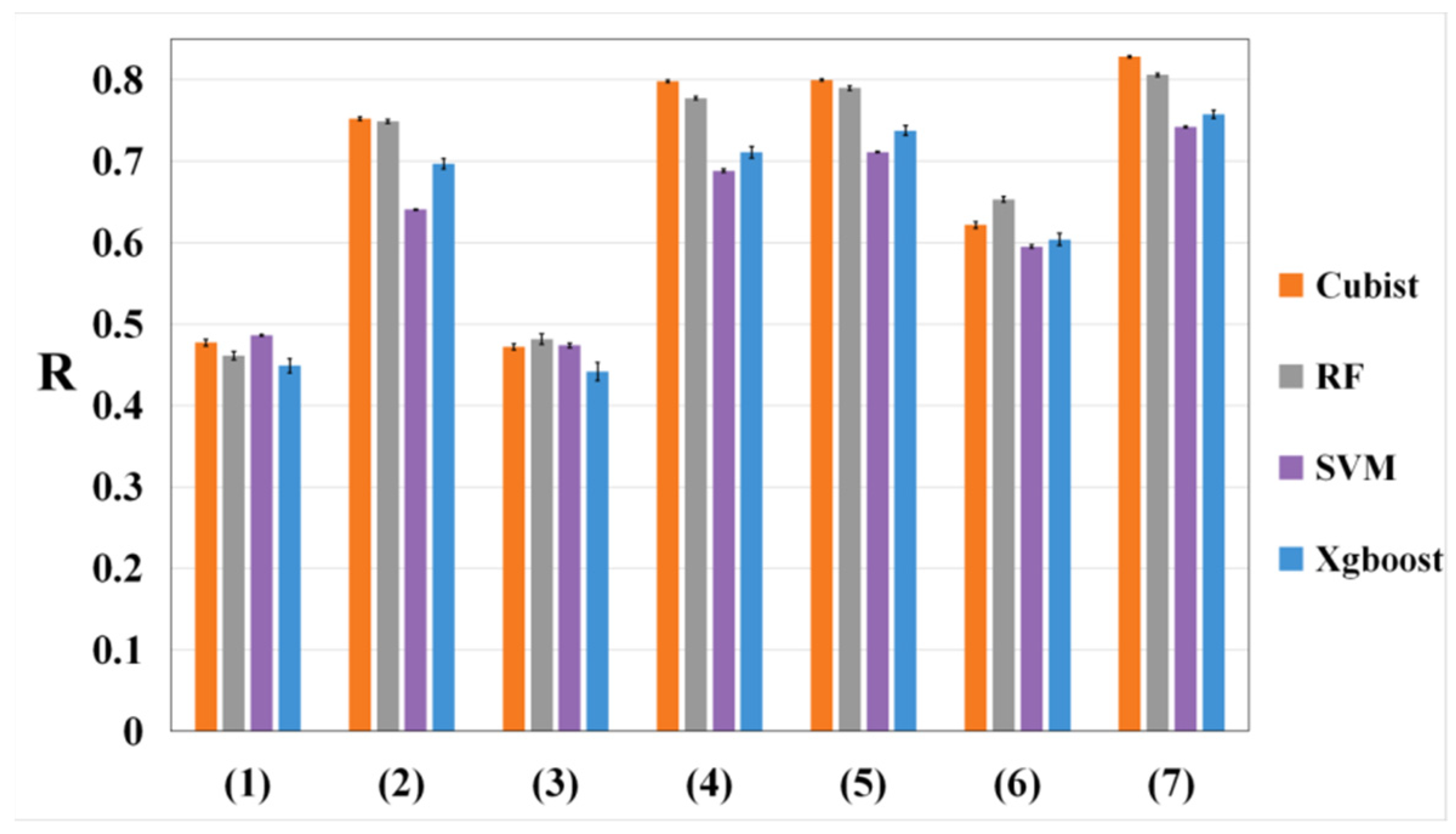
The study included three groups of experiments (Figure 2). The first group was designed to analyze which combination form would obtain the best performance, and we adopted nine combinations of inputs: (1) the satellite data (EVI, NDVI, and SAVI), (2) climate data only, (3) meteorological indices only, (4) climate and satellite data (EVI, NDVI, and SAVI); (5) climate data and the meteorological indices, (6) satellite data (EVI, NDVI, and SAVI) and the meteorological indices, and (7) climate, satellite data (EVI, NDVI, and SAVI) and the meteorological indices.
The second group was to test how climate, meteorological indices and satellite data from three growing periods contributed to maize yield prediction. The growing stages were defined as (1) the early growing period (March and April), (2) the peak growing period (May and June), and (3) the late growing period (July and August). The performance of climate data and meteorological indices from all stages and satellite data from specific stages, climate data from specific stages and satellite data and meteorological indices from all stages, as well as meteorological indices from specific stages and climate and satellite data from all stages, were compared.
The third group was designed to explore the spatial divergences of the model performance. For five maize-growing regions, the climate, satellite data, and meteorological indices were used to predict the maize yield.
Finally, the leave-one-out prediction method, which uses one year for testing and the rest for training to validate the performance of the model, was conducted.
3. Results
3.1. Selection of Climate Variables
The EDA results are shown in Figure 3. The water supply-related variables and temperature-related variables were negatively correlated with maize yield, whereas the Vpd of the water demand-related variables was positively correlated with maize yield. Among all water supply-related variables, the R between Wet and maize yield was the highest. Additionally, the R between Wet and Cld, Wet and Pre were above 0.5, so Cld and Pre were not selected. Among the three temperature-related variables, the Tmn was selected for the highest correlation coefficient with maize yield. All the water demand-related variables were selected, as the R between Vap and Pet, Vap and Vpd was below 0.5. Moreover, the results showed that maize yield was negatively related to PDf and SDf; conversely, maize yield was positively related to PDr and SDr. This was consistent with Tollenaar et al. [69], which showed that 27% of the maize yield change between 1984 and 2013 was attributable to solar brightening. Among the four radiation-related variables, the SDr had the highest correlation coefficient with maize yield. The R between other variables and SDr were below 0.5 except PDr, thus, PDf, SDf, and SDr were selected to apply in the machine learning methods. Finally, eight climate variables (Wet, Tmn, Pet, Vap, Vpd, PDf, SDf, and SDr) were selected out of the 13 variables to represent climate conditions.
3.2. Multi-Model Performances When Estimating Maize Yield
The first group of experiments used different combinations of climate, satellite data, and meteorological indices to evaluate model performance. The prediction performances of the seven forms of data inputs were evaluated across four machine learning algorithms (Figure 4). The results showed that the combination of climate, satellite data, and meteorological indices achieved the best performance, with R values ranging from 0.742 to 0.828. Indeed, the combination of the climate data and meteorological indices performed best, following by the combination of climate data with satellite data and the combination of meteorological indices with satellite data. Additionally, the performance of climate data only, with R values between 0.641 and 0.752, was better than that of satellite data only and meteorological indices only, with the lowest R values ranging from 0.460 to 0.487 0.449 to 0.486, respectively. Furthermore, the analyses clearly showed that the cubist model generally provided the best accuracy among the four learning methods in estimating R, followed by RF, Xgboost, and SVM.
3.3. The Divergences of Model Performances between Different Growth Stages and Maize-Growing Regions
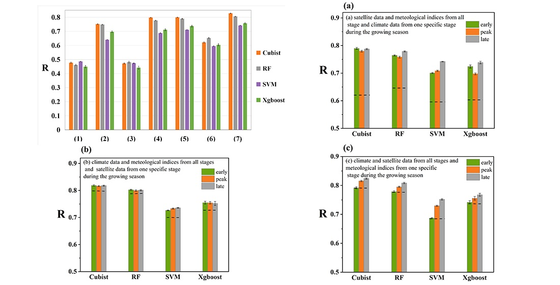
The yield forecasting performances using satellite data and meteorological indices from all periods and climate data from one specific period during the growing season were compared with those using satellite data from different periods and climate data and meteorological indices from all periods or meteorological indices from one specific period and climate and satellite data from all stages. R improved by about 0.126, 0.117, and 0.143 by adding climate data from the early, peak, and late periods to satellite data and meteorological indices from all stage via the four machine learning algorithms, respectively. R increased by 0.016, 0.016, and 0.017 when adding satellite data from the early, peak and late stages to climate data and meteorological indices from all stages, respectively. R increased by 0.003, 0.032, and 0.042 when adding meteorological indices from the early, peak and late periods to climate and satellite data from all stages, respectively (Figure 5).
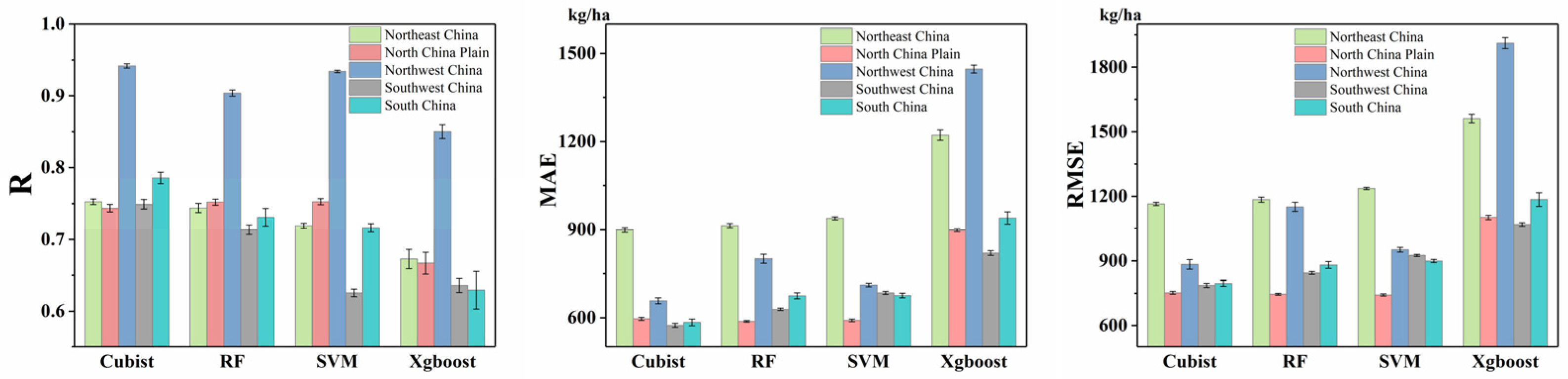
The result of the third experiment is shown in Figure 6. According to the model performance results, the R-value in Northwest China regions was much higher than that in other regions. In the Northwest China region, the R reached 0.941, 0.904, 0.934, and 0.850 for the cubist, RF, SVM, and Xgboost, respectively. The divergences between Northeast China, North China Plain, and South China were insignificant, ranging from 0.744 to 0.786, 0.731 to 0.752, 0.716 to 0.752, and 0.629 to 0.673 for the cubist, RF, SVM, and Xgboost, respectively. Moreover, the model performance was worst in Southwest China, where the R-value reached 0.749, 0.714, 0.626, and 0.636 for the cubist, RF, SVM, and Xgboost, respectively. The mean absolute error (MAE) and RMSE were low in North China Plain and Southwest China, with 668.22 and 676.89 kg/ha, and 835.66 and 906.10 kg/ha, respectively, across four machine learning methods. The MAE and RMSE values were 899.15 and 1164 kg/ha for cubist in Northeast China, whereas the highest MAE and RMSE occurred in Northwest China with the value of 904.09 and 1224.85 kg/ha.
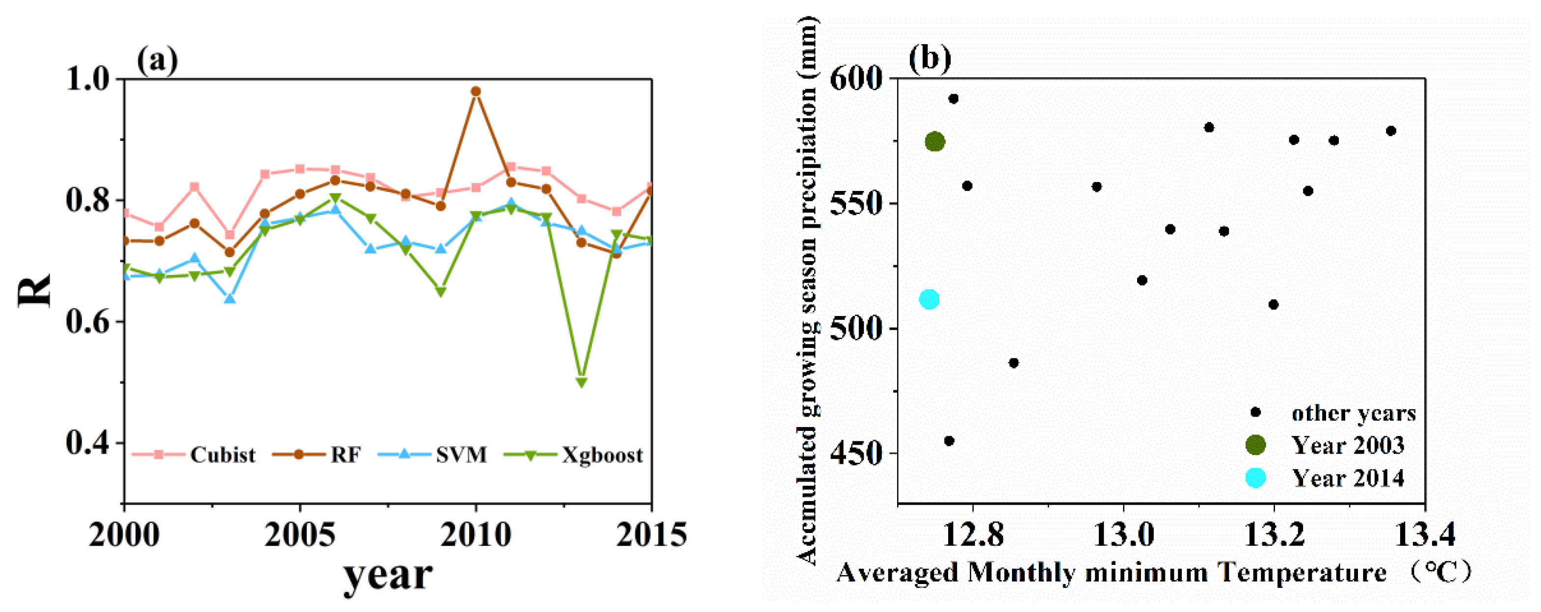
A leave-one-out test was executed to assess the robustness of the model. Prediction accuracy of different years clearly had some differences in different years. Most years showed great prediction accuracy except for 2003 and 2014 (Figure 7). According to the monthly minimum temperature and accumulated precipitation during the maize growing season, the results showed that the mean monthly temperature in 2003 and 2014 was lower than that in other years. The EDD was considered in the study; however, the extremely low temperature was ignored.
4. Discussion
4.1. Quantifying the Contributions of Climate, Satellite Data, and Meteorological Indices in Different Growth Stages to Maize Yield
Generally, the results indicated that the climate data, satellite data, and meteorological indices over the whole maize growing period played critical roles in determining maize growth and final maize yield. The highest estimated R values for the cubist, RF, SVM, and Xgboost methods were 0.828, 0.806, 0.742, and 0.758, respectively. The cubist algorithm achieved the best performance among four machine learning methods, achieving an R of 0.828 by combining climate, satellite data, and meteorological indices in this study; however, the value was relatively lower than that of Jiang et al. [5] with a value of 0.872. They used a long short-term memory (LSTM) model by integrating heterogeneous crop phenology, meteorology, and remote sensing data to estimate country-level maize yield across the US Corn Belt from 2006 to 2016. The reasons for the slight divergences in R were as follows: (1) this study was conducted in China, while the study of Jiang et al. [47] was conducted in the US Corn Belt. The main maize cropping regions belong to a monsoon climate or subordinate temperate continental climate in China, however, the US Corn Belt belongs to a temperate continental climate zone, where rainfall is less and concentrated, and the continental climate is strong; (2) this study was conducted for a longer period of 2000 to 2015 than that from 2006 to 2016. The R of combining climate and meteorological indices reached 0.80, 0.79, 071, and 0.72 for the cubist, RF, SVM, and Xgboost, respectively. This result was similar to the previous study of Chen et al. [70], which indicated that climate change and extreme climate could account for 56.7% of maize yield change by applying a stepwise regression.
The results also showed that the prediction skill of satellite data and meteorological indices for all stages and climate data for the late-stage was better than that from the early and peak stages of the four machine learning methods. Additionally, the prediction skill of climate and satellite data for all stages and meteorological indices for the late-stage was better than that for the early and peak stage. Specifically, R improved by about 0.126, 0.117, and 0.143 by adding climate data from the early, peak, and late periods to satellite data and meteorological indices from all stages via the four machine learning algorithms, respectively. R increased by 0.016, 0.016, and 0.017 when adding satellite data from the early, peak, and late stages to climate data and meteorological indices from all stages, respectively. R increased by 0.003, 0.032, and 0.042 when adding meteorological indices from the early, peak, and late stages to climate and satellite data from all stages, respectively. These were in agreement with the result of Karimi et al. [42], which showed that the RMSE values at the tasseling stage were lower than those at the early growth stage. They also found the R values between the observed and simulated yields at the tasseling stage were much higher than those calculated for the early growth stage by using the SVM algorithm. This study was also consistent with previous studies [71,72], which noted that crop yield was highly correlated with biomass during the ripening stage or grain filling period. This phenomenon might contribute to crop sensitivities to different climatic events varying with the growth phase [73]. For example, according to Daryanto et al. [74], maize was more sensitive to drought during the reproductive phase than during the vegetative phase. In contrast, the difference was not obvious between satellite data in the three stages and climate data and meteorological indices over the whole maize growing stages. The results also revealed that the added value of satellite data given climate data and meteorological indices over the maize growing season, as well as the value of meteorological data given climate and satellite data in the whole growing season, was smaller than the value of climate data given satellite data and meteorological indices over the maize growing season. Indeed, the performance of the model could slightly improve the R-value to a level that was impossible to reach by climate information alone. This finding was in agreement with the results of Becker-Reshef et al. [43] and Kern et al. [75], who found that the model performance was greatly improved by adding satellite information to climate data. According to Son et al. [31], crop biomass at different phenological periods had different correlation levels with different VIs, which might be attributed to the phenological variations in plant growth related to the change in climatic conditions [76,77].
4.2. Quantifying the Divergences of Model Performances Between Five Maize-Growing Regions
The spatial divergences of R value between different maize-growing regions were obvious. Indeed, the R-value in Northwest China region was significantly higher than that in other regions. The divergence might be attributed to Northwest China having a continental climate, which is characterized by a dry climate and sufficient sunshine. Besides, the population density in this region is small, with less interference from human activities compared to other regions. The reason for the poor model performance in the Southwest China region might be that this region has a temperate humid climate, which is characterized by abundant rainfall and less sunshine. Additionally, climate changes are more complicated in this region. Therefore, for regions with similar climate characteristics to Northwest China, the maize yield prediction method in this study was efficient and useful. Yao et al. [40] estimated the maize yield by using a process-based model in the Northeast China Plain during 2002–2011. Their results showed that the R and RMSE were 0.827 and 712 kg/ha, respectively, from 2002 to 2011. The results were slightly better than those in this study, however, this might be attributable to the process-based model being superior in small-scale than large-scale regions. However, machine learning methods were widely and well used in large-scale regions.
The leave-one-out test showed great prediction accuracy in most years except for 2003 and 2014. The EDD was considered in the study, however, the extreme low temperature was ignored. This result was consistent with that of Li et al. [11] and Cai et al. [29], who found that extreme climate was another factor affecting yield predictability. However, our results showed good performances throughout the year, which had extremely low precipitation. This might be attributed to the fact that the prediction could be greatly improved by incorporating satellite data that could contain crop progress information [11]. Hence, this study showed that the machine learning models had limited in predicting maize yield when extreme climate conditions existed. These extreme climate events could cause large prediction biases due to that such conditions might not have occurred in the historic training dataset.
4.3. Uncertainty and Limitations
This study successfully applied four machine learning approaches to predict maize yield in China. Three limitations of this work should be considered. Firstly, although the SAVI was added to consider soil property information, uncertainties in the heterogeneity of environmental conditions might be ignored [78], including irrigation system, fertilizer application rate, and soil conditions. Secondly, as our models were built on a fixed growth season, crop phenology dynamics were ignored in this study. Hence, further studies should consider the crop phenology of each statistical unit to improve the prediction accuracy. Finally, all the machine learning methods that function as black boxes were nonlinear methods with the characteristic of limited process-based interpretation. Moreover, the mechanism of each method also had divergences, thus, a more accurate machine learning method will improve the performance of maize prediction.
5. Conclusions
In this study, four machine learning approaches, including cubist, Xgboost, RF, and SVM, were used to predict maize yield at the city level in China from 2000 to 2015 based on climate, satellite data, and meteorological indices. This study included three groups of experiments. The first group adopted seven combinations of inputs to analyze which combination would obtain the best performance. The second group was used to test how climate data, meteorological indices, and satellite data from different growing periods contributed to maize yield prediction, and the third group was designed to explore the model performance differences of five maize-growing regions. The major findings were as follows:
- (1)
- The performance of climate data, with R ranging from 0.641 to 0.752, was better than that of satellite data and meteorological indices, with the lowest R ranging from 0.449 to 0.486 and 0.442 to 0.481, respectively. Integrating all climate, satellite data, and meteorological indices could achieve the highest accuracy.
- (2)
- The climate data or satellite data inputs from all growth stages were essential for maize yield prediction, especially in late growth stages.
- (3)
- The spatial analysis found that the spatial divergences were large, and the R-value in the Northwest region reached 0.942, 0.904, 0.934, and 0.850 for the Cubist, RF, SVM, and Xgboost, respectively. Additionally, unprecedented extreme climate events could cause large prediction biases.
In summary, this study provided an applicable approach using climate, satellite data, and meteorological indices for large-scale yield prediction, which could be used for other crop types and other regions.
Author Contributions
Conceptualization, L.F.; Data curation, X.C. and R.Y.; Formal analysis, X.C. and X.W.; Funding acquisition, W.G.; Investigation, J.S.; Methodology, L.F.; Project administration, L.F.; Writing—original draft, X.C. All authors have read and agreed to the published version of the manuscript.
Funding
This work was financially supported by the National Natural Science Foundation of China (No. 41975044, No. 41801021, 41871019,41672355), and the Special Fund for Basic Scientific Research of Central Colleges, China University of Geosciences, Wuhan (No. CUGL170401 and CUGCJ1704). We would like to thank the China Meteorological Administration (CMA) for providing the meteorological data.
Conflicts of Interest
The authors declare no conflict of interest.
References
- Kuwata, K.; Shibasaki, R. Estimating corn yield in the United States with modis evi and machine learning methods. ISPRS Ann. Photogramm. Remote Sens. Spat. Inf. Sci. 2016, III-8, 131–136. [Google Scholar] [CrossRef]
- Pantazi, X.E.; Moshou, D.; Alexandridis, T.; Whetton, R.L.; Mouazen, A.M. Wheat yield prediction using machine learning and advanced sensing techniques. Comput. Electron. Agric. 2016, 121, 57–65. [Google Scholar] [CrossRef]
- Morell, F.J.; Yang, H.S.; Cassman, K.G.; Wart, J.V.; Elmore, R.W.; Licht, M.; Coulter, J.A.; Ciampitti, I.A.; Pittelkow, C.M.; Brouder, S.M.; et al. Can crop simulation models be used to predict local to regional maize yields and total production in the U.S. Corn Belt? Field Crops Res. 2016, 192, 1–12. [Google Scholar] [CrossRef] [Green Version]
- Everingham, Y.L.; Smyth, C.W.; Inman-Bamber, N.G. Ensemble data mining approaches to forecast regional sugarcane crop production. Agric. For. Meteorol. 2009, 149, 689–696. [Google Scholar] [CrossRef]
- Lecerf, R.; Ceglar, A.; López-Lozano, R.; Van Der Velde, M.; Baruth, B. Assessing the information in crop model and meteorological indicators to forecast crop yield over Europe. Agric. Syst. 2019, 168, 191–202. [Google Scholar] [CrossRef]
- Maharjan, G.R.; Hoffmann, H.; Webber, H.; Srivastava, A.K.; Weihermüller, L.; Villa, A.; Coucheney, E.; Lewan, E.; Trombi, G.; Moriondo, M.; et al. Effects of input data aggregation on simulated crop yields in temperate and Mediterranean climates. Eur. J. Agron. 2019, 103, 32–46. [Google Scholar] [CrossRef]
- Gilardelli, C.; Stella, T.; Confalonieri, R.; Ranghetti, L.; Campos-Taberner, M.; García-Haro, F.J.; Boschetti, M. Downscaling rice yield simulation at sub-field scale using remotely sensed LAI data. Eur. J. Agron. 2019, 103, 108–116. [Google Scholar] [CrossRef]
- Leroux, L.; Castets, M.; Baron, C.; Escorihuela, M.; Bégué, A.; Lo Seen, D. Maize yield estimation in West Africa from crop process-induced combinations of multi-domain remote sensing indices. Eur. J. Agron. 2019, 108, 11–26. [Google Scholar] [CrossRef]
- Pagani, V.; Guarneri, T.; Fumagalli, D.; Movedi, E.; Testi, L.; Klein, T.; Calanca, P.; Villalobos, F.; Lopez-Bernal, A.; Niemeyer, S.; et al. Improving cereal yield forecasts in Europe—The impact of weather extremes. Eur. J. Agron. 2017, 89, 97–106. [Google Scholar] [CrossRef]
- Balaghi, R.; Tychon, B.; Eerens, H.; Jlibene, M. Empirical regression models using NDVI, rainfall and temperature data for the early prediction of wheat grain yields in Morocco. Int. J. Appl. Earth Obs. 2008, 10, 438–452. [Google Scholar] [CrossRef] [Green Version]
- Li, Y.; Guan, K.; Yu, A.; Peng, B.; Zhao, L.; Li, B.; Peng, J. Toward building a transparent statistical model for improving crop yield prediction: Modeling rainfed corn in the U.S. Field Crops Res. 2019, 234, 55–65. [Google Scholar] [CrossRef]
- Bussay, A.; van der Velde, M.; Fumagalli, D.; Seguini, L. Improving operational maize yield forecasting in Hungary. Agric. Syst. 2015, 141, 94–106. [Google Scholar] [CrossRef]
- Peng, B.; Guan, K.; Pan, M.; Li, Y. Benefits of Seasonal Climate Prediction and Satellite Data for Forecasting U.S. Maize Yield. Geophys. Res. Lett. 2018, 45, 9662–9671. [Google Scholar] [CrossRef]
- Mathieu, J.A.; Aires, F. Statistical Weather-Impact Models: An Application of Neural Networks and Mixed Effects for Corn Production over the United States. J. Appl. Meteorol. Clim. 2016, 55, 2509–2527. [Google Scholar] [CrossRef]
- Jones, J.W.; Antle, J.M.; Basso, B.; Boote, K.J.; Conant, R.T.; Foster, I.; Godfray, H.C.J.; Herrero, M.; Howitt, R.E.; Janssen, S.; et al. Brief history of agricultural systems modeling. Agric. Syst. 2017, 155, 240–254. [Google Scholar] [CrossRef]
- Johnson, M.D.; Hsieh, W.W.; Cannon, A.J.; Davidson, A.; Bédard, F. Crop yield forecasting on the Canadian Prairies by remotely sensed vegetation indices and machine learning methods. Agric. Forest Meteorol. 2016, 218–219, 74–84. [Google Scholar] [CrossRef]
- Schwalbert, R.A.; Amado, T.; Corassa, G.; Pott, L.P.; Prasad, P.V.V.; Ciampitti, I.A. Satellite-based soybean yield forecast: Integrating machine learning and weather data for improving crop yield prediction in southern Brazil. Agric. Forest Meteorol. 2020, 284, 107886. [Google Scholar] [CrossRef]
- Crane-Droesch, A. Machine learning methods for crop yield prediction and climate change impact assessment in agriculture. Environ. Res. Lett. 2018, 13, 1–12. [Google Scholar] [CrossRef] [Green Version]
- Alvarez, R. Predicting average regional yield and production of wheat in the Argentine Pampas by an artificial neural network approach. Eur. J. Agron. 2009, 30, 70–77. [Google Scholar] [CrossRef]
- Chlingaryan, A.; Sukkarieh, S.; Whelan, B. Machine learning approaches for crop yield prediction and nitrogen status estimation in precision agriculture: A review. Comput. Electron. Agric. 2018, 151, 61–69. [Google Scholar] [CrossRef]
- Cai, Y.; Guan, K.; Peng, J.; Wang, S.; Seifert, C.; Wardlow, B.; Li, Z. A high-performance and in-season classification system of field-level crop types using time-series Landsat data and a machine learning approach. Remote Sens. Environ. 2018, 210, 35–47. [Google Scholar] [CrossRef]
- Peiris, T.S.G.; Hansen, J.W.; Zubair, L. Use of seasonal climate information to predict coconut production in Sri Lanka. Int. J. Climatol. 2008, 28, 103–110. [Google Scholar] [CrossRef] [Green Version]
- Martinez, C.J.; Baigorria, G.A.; Jones, J.W. Use of climate indices to predict corn yields in southeast USA. Int. J. Climatol. 2009, 29, 1680–1691. [Google Scholar] [CrossRef]
- Holzman, M.E.; Carmona, F.; Rivas, R.; Niclòs, R. Early assessment of crop yield from remotely sensed water stress and solar radiation data. ISPRS J. Photogramm. 2018, 145, 297–308. [Google Scholar] [CrossRef]
- Holzman, M.E.; Rivas, R.E. Early Maize Yield Forecasting From Remotely Sensed Temperature/Vegetation Index Measurements. IEEE J. STARS 2016, 9, 507–519. [Google Scholar] [CrossRef]
- Wang, L.; Tian, Y.; Yao, X.; Zhu, Y.; Cao, W. Predicting grain yield and protein content in wheat by fusing multi-sensor and multi-temporal remote-sensing images. Field Crops Res. 2014, 164, 178–188. [Google Scholar] [CrossRef]
- Bolton, D.K.; Friedl, M.A. Forecasting crop yield using remotely sensed vegetation indices and crop phenology metrics. Agric. Forest Meteorol. 2013, 173, 74–84. [Google Scholar] [CrossRef]
- Franch, B.; Vermote, E.F.; Becker-Reshef, I.; Claverie, M.; Huang, J.; Zhang, J.; Justice, C.; Sobrino, J.A. Improving the timeliness of winter wheat production forecast in the United States of America, Ukraine and China using MODIS data and NCAR Growing Degree Day information. Remote Sens. Environ. 2015, 161, 131–148. [Google Scholar] [CrossRef]
- Cai, Y.; Guan, K.; Lobell, D.; Potgieter, A.B.; Wang, S.; Peng, J.; Xu, T.; Asseng, S.; Zhang, Y.; You, L.; et al. Integrating satellite and climate data to predict wheat yield in Australia using machine learning approaches. Agric. Forest Meteorol. 2019, 274, 144–159. [Google Scholar] [CrossRef]
- Chen, C.F.; Son, N.T.; Chen, C.R.; Chiang, S.H.; Chang, L.Y.; Valdez, M. Drought monitoring in cultivated areas of Central America using multi-temporal MODIS data. Geomat. Nat. Hazards Risk 2017, 8, 402–417. [Google Scholar] [CrossRef] [Green Version]
- Son, N.T.; Chen, C.F.; Chen, C.R.; Minh, V.Q.; Trung, N.H. A comparative analysis of multitemporal MODIS EVI and NDVI data for large-scale rice yield estimation. Agric. For. Meteorol. 2014, 197, 52–64. [Google Scholar] [CrossRef]
- Deng, F.; Su, G.; Liu, C. Seasonal Variation of MODIS Vegetation Indexes and Their Statistical Relationship with Climate Over the Subtropic Evergreen Forest in Zhejiang, China. IEEE Geosci. Remote S 2007, 4, 236–240. [Google Scholar] [CrossRef]
- Gontia, N.K.; Tiwari, K.N. Yield Estimation Model and Water Productivity of Wheat Crop (Triticum aestivum) in an Irrigation Command Using Remote Sensing and GIS. J. Indian Soc. Remote 2011, 39, 27–37. [Google Scholar] [CrossRef]
- Guo, C.; Tang, Y.; Lu, J.; Zhu, Y.; Cao, W.; Cheng, T.; Zhang, L.; Tian, Y. Predicting wheat productivity: Integrating time series of vegetation indices into crop modeling via sequential assimilation. Agric. For. Meteorol. 2019, 272–273, 69–80. [Google Scholar] [CrossRef]
- Panda, S.S.; Ames, D.P.; Panigrahi, S. Application of Vegetation Indices for Agricultural Crop Yield Prediction Using Neural Network Techniques. Remote Sens. 2010, 2, 673–696. [Google Scholar] [CrossRef] [Green Version]
- Pede, T.; Mountrakis, G.; Shaw, S.B. Improving corn yield prediction across the US Corn Belt by replacing air temperature with daily MODIS land surface temperature. Agric. For. Meteorol. 2019, 276–277, 107615. [Google Scholar] [CrossRef]
- Feng, P.; Wang, B.; Liu, D.; Waters, C.; Xiao, D.; Shi, L.; Yu, Q. Dynamic wheat yield forecasts are improved by a hybrid approach using a biophysical model and machine learning technique. Agric. For. Meteorol. 2020, 285–286, 107922. [Google Scholar] [CrossRef]
- Mo, X.; Liu, S.; Lin, Z.; Xu, Y.; Xiang, Y.; McVicar, T.R. Prediction of crop yield, water consumption and water use efficiency with a SVAT-crop growth model using remotely sensed data on the North China Plain. Ecol. Model. 2005, 183, 301–322. [Google Scholar] [CrossRef]
- Huang, J.; Wang, X.; Li, X.; Tian, H.; Pan, Z. Remotely sensed rice yield prediction using multi-temporal NDVI data derived from NOAA’s-AVHRR. PLoS ONE 2013, 8, e70816. [Google Scholar] [CrossRef]
- Yao, F.; Tang, Y.; Wang, P.; Zhang, J. Estimation of maize yield by using a process-based model and remote sensing data in the Northeast China Plain. Phys. Chem. Earth Parts A/B/C 2015, 87–88, 142–152. [Google Scholar] [CrossRef]
- Yao, R.; Wang, L.; Huang, X.; Li, L.; Sun, J.; Wu, X.; Jiang, W. Developing a temporally accurate air temperature dataset for Mainland China. Sci. Total Environ. 2020, 706, 136037. [Google Scholar] [CrossRef] [PubMed]
- Karimi, Y.; Prasher, S.O.; Madani, A.; Kim, S. Application of support vector machine technology for the estimation of crop biophysical parameters using aerial hyperspectral observations. Can. Biosyst. Eng. 2008, 50, 13–20. [Google Scholar]
- Becker-Reshef, I.; Vermote, E.; Lindeman, M.; Justice, C. A generalized regression-based model for forecasting winter wheat yields in Kansas and Ukraine using MODIS data. Remote Sens. Environ. 2010, 114, 1312–1323. [Google Scholar] [CrossRef]
- FOASTAT. Food and Agriculture Organization; FOASTAT Database: New York, NY, USA, 2017. [Google Scholar]
- You, L.; Wood, S.; Wood-sichra, U. Generating global crop distribution maps: From census to grid. Agric. Syst. 2014, 127, 53–60. [Google Scholar] [CrossRef] [Green Version]
- Jones, P.D.; Harris, I.C. Climatic Research Unit (CRU): Time-Series (TS) Datasets of Variations in Climate with Variations in Other Phenomena v3; University of East Anglia Climatic Research Unit, NCAS British Atmospheric Data Centre: Leeds, UK, 2008. [Google Scholar]
- Jiang, H.; Hu, H.; Zhong, R.; Xu, J.; Xu, J.; Huang, J.; Wang, S.; Ying, Y.; Lin, T. A deep learning approach to conflating heterogeneous geospatial data for corn yield estimation: A case study of the US Corn Belt at the county level. Glob. Chang. Biol. 2020, 26, 1754–1766. [Google Scholar] [CrossRef] [PubMed]
- Butler, E.E.; Huybers, P. Adaptation of US maize to temperature variations. Nat. Clim. Chang. 2013, 3, 68–72. [Google Scholar] [CrossRef]
- Mishra, A.K.; Singh, V.P. Drought modeling—A review. J. Hydrol. 2011, 403, 157–175. [Google Scholar] [CrossRef]
- Zuo, D.; Cai, S.; Xu, Z.; Peng, D.; Kan, G.; Sun, W.; Pang, B.; Yang, H. Assessment of meteorological and agricultural droughts using in-situ observations and remote sensing data. Agric. Water Manag. 2019, 222, 125–138. [Google Scholar] [CrossRef]
- Zhang, F.; Yanan, C.; Jiquan, Z.; Enliang, G.; Wang, R.; Li, D. Dynamic drought risk assessment for maize based on crop simulation model and multi-source drought indices. J. Clean. Prod. 2019, 233, 100–114. [Google Scholar] [CrossRef]
- Fu, J.; Niu, J.; Kang, S.; Adeloye, A.J.; Du, T. Crop production in the Hexi Corridor challenged by future climate change. J. Hydrol. 2019, 579, 124197. [Google Scholar] [CrossRef]
- Quinlan, R. Learning with continuous classes. Aust. Jt. Conf. Artif. Intell. 1992, 92, 343–348. [Google Scholar]
- Houborg, R.; McCabe, M.F. A hybrid training approach for leaf area index estimation via Cubist and random forests machine-learning. ISPRS J. Photogramm. 2018, 135, 173–188. [Google Scholar] [CrossRef]
- Johnson, D.M. An assessment of pre- and within-season remotely sensed variables for forecasting corn and soybean yields in the United States. Remote Sens. Environ. 2014, 141, 116–128. [Google Scholar] [CrossRef]
- Kuhn, M.; Weston, S.; Keefer, C.; Counlter, N. Cubist Models for Regression. 2012. Available online: https://mran.microsoft.com/snapshot/2016-09-15/web/packages/Cubist/vignettes/cubist.pdf (accessed on 25 December 2020).
- LV, Y.; Le, Q.; Bui, H.; Bui, X.; Nguyen, H.; Nguyen-Thoi, T.; Dou, J.; Song, X. A Comparative Study of Different Machine Learning Algorithms in Predicting the Content of Ilmenite in Titanium Placer. Appl. Sci. 2020, 10, 635. [Google Scholar] [CrossRef] [Green Version]
- Breiman, L. Random Forests. Mach. Learn. 2001, 45, 5–32. [Google Scholar] [CrossRef] [Green Version]
- Adam, E.M.I.; Mutanga, O. Estimation of high density wetland biomass: Combining regression model with vegetation index developed from Worldview-2 imagery. In Proceedings of the SPIE, Edinburgh, UK, 24–27 September 2012; Volume 8531, p. 85310V. [Google Scholar]
- Tulbure, M.G.; Wimberly, M.C.; Boe, A.; Owens, V.N. Climatic and genetic controls of yields of switchgrass, a model bioenergy species. Agric. Ecosyst. Environ. 2012, 146, 121–129. [Google Scholar] [CrossRef]
- Everingham, Y.; Sexton, J.; Skocaj, D.; Inman-Bamber, G. Accurate prediction of sugarcane yield using a random forest algorithm. Agron. Sustain. Dev. 2016, 36, 27. [Google Scholar] [CrossRef] [Green Version]
- Prasad, A.M.; Iverson, L.R.; Liaw, A. Newer Classification and Regression Tree Techniques: Bagging and Random Forests for Ecological Prediction. Ecosystems 2006, 9, 181–199. [Google Scholar] [CrossRef]
- Chen, T.; Guestrin, C. XGBoost: A Scalable Tree Boosting System. In Proceedings of the 22nd Acm Sigkdd International Conference on Knowledge Discovery and Data Mining, San Francisco, CA, USA, 13–17 August 2016; pp. 785–794. [Google Scholar]
- Zhang, L.; Ai, H.; Chen, W.; Yin, Z.; Hu, H.; Zhu, J.; Zhao, J.; Zhao, Q.; Liu, H. CarcinoPred-EL: Novel models for predicting the carcinogenicity of chemicals using molecular fingerprints and ensemble learning methods. Sci. Rep. 2017, 7, 2118. [Google Scholar] [CrossRef]
- Cortes, C.; Vapink, A. Support-Vector Networks. Mach. Learn. 1995, 20, 273–297. [Google Scholar] [CrossRef]
- Brdar, S.; Culibrk, D.; Marinkovic, B.; Crnobaracy, J.; Crnojevic, V. Support Vector Machines with Features Contribution Analysis for Agricultural Yield Prediction. In Proceedings of the Second International Workshop on Sensing Technologies in Agriculture, Forestry and Environment (EcoSense 2011), Belgrade, Serbia, 6–7 April 2011; pp. 43–47. [Google Scholar]
- Cai, Y.D.; Ricardo, P.W.; Jen, C.H.; Chou, K.C. Application of SVM to predict membrane protein types. J. Theor. Biol. 2004, 226, 373–376. [Google Scholar] [CrossRef] [Green Version]
- Bermolen, P.; Rossi, D. Support vector regression for link load prediction. Comput. Netw. 2009, 53, 191–201. [Google Scholar] [CrossRef]
- Tollenaar, M.; Fridgen, J.; Tyagi, P.; Stackhouse, P.W., Jr.; Kumudini, S. The contribution of solar brightening to the US maize yield trend. Nat. Clim. Chang. 2017, 7, 275–278. [Google Scholar] [CrossRef]
- Chen, X.; Wang, L.; Niu, Z.; Zhang, M.; Li, C.; Li, J. The effects of projected climate change and extreme climate on maize and rice in the Yangtze River Basin, China. Agric. For. Meteorol. 2020, 282–283, 107867. [Google Scholar] [CrossRef]
- Son, N.T.; Chen, C.F.; Chen, C.R.; Chang, L.Y.; Duc, H.N.; Nguyen, L.D. Prediction of rice crop yield using MODIS EVI−LAI data in the Mekong Delta, Vietnam. Int. J. Remote Sens. 2013, 34, 7275–7292. [Google Scholar] [CrossRef]
- Benedetti, R.; Rossini, P. On the use of NDVI profiles as a tool for agricultural statistics: The case study of wheat yield estimate and forecast in Emilia Romagna. Remote Sens. Environ. 1993, 45, 311–326. [Google Scholar] [CrossRef]
- Sánchez, B.; Rasmussen, A.; Porter, J.R. Temperatures and the growth and development of maize and rice: A review. Glob. Chang. Biol. 2014, 20, 408–417. [Google Scholar] [CrossRef]
- Daryanto, S.; Wang, L.; Jacinthe, P. Global Synthesis of Drought Effects on Maize and Wheat Production. PLoS ONE 2016, 11, e156362. [Google Scholar] [CrossRef]
- Kern, A.; Barcza, Z.; Marjanović, H.; Árendás, T.; Fodor, N.; Bónis, P.; Bognár, P.; Lichtenberger, J. Statistical modelling of crop yield in Central Europe using climate data and remote sensing vegetation indices. Agric. For. Meteorol. 2018, 260–261, 300–320. [Google Scholar] [CrossRef]
- Wang, Q.; Adiku, S.; Tenhunen, J.; Granier, A. On the relationship of NDVI with leaf area index in a deciduous forest site. Remote sensing of environment. Remote Sens. Environ. 2005, 94, 244–255. [Google Scholar] [CrossRef]
- Cohen, W.B.; Maiersperger, T.K.; Gower, S.T.; Turner, D.P. An improved strategy for regression of biophysical variables and Landsat ETM+ data. Remote Sens. Environ. 2003, 84, 561–571. [Google Scholar] [CrossRef] [Green Version]
- Conradt, S.; Bokusheva, R.; Finger, R.; Kussaiynov, T. Yield Trend Estimation in the Presence of Farm Heterogeneity and Non-linear Technological Change. Q. J. Int. Agric. 2014, 53, 121–140. [Google Scholar]
Figure 1.
The maize cropping regions in China.

Figure 2.
Flowchart indicating all steps of the model development.

Figure 3.
Exploratory data analysis (EDA) results showing the correlations among 13 variables and correlations (R) between each climate variable and maize yield (statistical significance was tested using single-factor analysis of variance, p < 0.05). The color and size of the dots indicate the correlation strength. The low correlations (p > 0.05) were not displayed in the figure.

Figure 4.
The model performances (estimated R values) of the different methods include combinations: (1) satellite data (EVI, NDVI, and SAVI), (2) climate data, (3) meteorological indices, (4) climate and satellite data (EVI, NDVI, and SAVI), (5) climate data and meteorological indices, (6) satellite data (EVI, NDVI, and SAVI) and meteorological indices; and (7) climate, satellite (EVI, NDVI, and SAVI) and meteorological indices, input for the whole growing season. The error bars are one standard deviation of predicted R from 10 ensembles by dividing the training and testing datasets randomly.

Figure 5.
(a) The R values using satellite data and meteorological indices for all stages but using climate data for only one stage of the maize growing season, which was divided into early (Mar and Apr), peak (May and Jun), and late (Jul and Aug) stages. (b) R values using climate data and meteorological indices for all stages but using satellite data for only one stage. (c) R values using climate and satellite data for all stages but using meteorological indices for only one stage. The dashed lines in (a–c) represent the benchmark model performance when using satellite data only, climate data only, and meteorological indices only during all stages, respectively.

Figure 6.
The model performances (estimated R values, mean absolute error (MAE), and root mean square error (RMSE)) of the different methods utilizing in five maize-growing regions. The error bars are one standard deviation of estimated R from 10 ensembles by dividing the training and testing datasets randomly.

Figure 7.
The leave-one-out experiment. (a) The performances of the different methods across 16 years. One-year data are selected for testing, while data from other years are utilized for training. (b) Scatter plot between the average monthly mean temperature and the accumulated growing season precipitation during the growing season across 16 years in China.


Table 1.
Information on average temperature, rainfall, daily diffuse flux of photosynthetic active radiation, potential evapotranspiration, and altitude for the five regions during maize growing season.
Table 1.
Information on average temperature, rainfall, daily diffuse flux of photosynthetic active radiation, potential evapotranspiration, and altitude for the five regions during maize growing season.
| Northeast China | North China Plain | Northwest China | Southwest China | South China | |
|---|---|---|---|---|---|
| Altitude (m) | 323.268 | 947.513 | 2358.135 | 3429.555 | 331.731 |
| Mean temperature in maize growing season (°C/day) | 14.320 | 19.912 | 15.776 | 19.523 | 21.715 |
| Precipitation (mm/month) | 67.307 | 81.762 | 29.284 | 129.170 | 137.058 |
| Potential evapotranspiration (mm/day) | 26.752 | 33.066 | 13.765 | 51.356 | 53.822 |
| Diffuse flux of photosynthetic active radiation (W m−2/day) | 59.922 | 62.902 | 62.8185 | 64.051 | 64.341 |
Publisher’s Note: MDPI stays neutral with regard to jurisdictional claims in published maps and institutional affiliations. |
© 2021 by the authors. Licensee MDPI, Basel, Switzerland. This article is an open access article distributed under the terms and conditions of the Creative Commons Attribution (CC BY) license (http://creativecommons.org/licenses/by/4.0/).
Share and Cite
MDPI and ACS Style
Chen, X.; Feng, L.; Yao, R.; Wu, X.; Sun, J.; Gong, W. Prediction of Maize Yield at the City Level in China Using Multi-Source Data. Remote Sens. 2021, 13, 146. https://0-doi-org.brum.beds.ac.uk/10.3390/rs13010146
AMA Style
Chen X, Feng L, Yao R, Wu X, Sun J, Gong W. Prediction of Maize Yield at the City Level in China Using Multi-Source Data. Remote Sensing. 2021; 13(1):146. https://0-doi-org.brum.beds.ac.uk/10.3390/rs13010146
Chicago/Turabian StyleChen, Xinxin, Lan Feng, Rui Yao, Xiaojun Wu, Jia Sun, and Wei Gong. 2021. "Prediction of Maize Yield at the City Level in China Using Multi-Source Data" Remote Sensing 13, no. 1: 146. https://0-doi-org.brum.beds.ac.uk/10.3390/rs13010146
Note that from the first issue of 2016, this journal uses article numbers instead of page numbers. See further details here.