SBAS-Aided GPS Positioning with an Extended Ionosphere Map at the Boundaries of WAAS Service Area


School of Aerospace and Mechanical Engineering, Korea Aerospace University, Goyang-si 10540, Gyeonggi-do, Korea
*
Author to whom correspondence should be addressed.
Remote Sens. 2021, 13(1), 151; https://0-doi-org.brum.beds.ac.uk/10.3390/rs13010151
Submission received: 6 November 2020
/
Revised: 29 December 2020
/
Accepted: 1 January 2021
/
Published: 5 January 2021
Abstract
:Space-based augmentation system (SBAS) provides correction information for improving the global navigation satellite system (GNSS) positioning accuracy in real-time, which includes satellite orbit/clock and ionospheric delay corrections. At SBAS service area boundaries, the correction is not fully available to GNSS users and only a partial correction is available, mostly satellite orbit/clock information. By using the geospatial correlation property of the ionosphere delay information, the ionosphere correction coverage can be extended by a spatial extrapolation algorithm. This paper proposes extending SBAS ionosphere correction coverage by using a biharmonic spline extrapolation algorithm. The wide area augmentation system (WAAS) ionosphere map is extended and its ionospheric delay error is compared with the GPS Klobuchar model. The mean ionosphere error reduction at low latitude is 52.3%. The positioning accuracy of the extended ionosphere correction method is compared with the accuracy of the conventional SBAS positioning method when only a partial set of SBAS corrections are available. The mean positioning error reduction is 44.8%, and the positioning accuracy improvement is significant at low latitude.
1. Introduction
Global navigation satellite system (GNSS) positioning accuracy is limited by various GNSS error sources; satellite orbit error, satellite clock error, and ionospheric delay among others. External correction data can be used to reduce the effect of those error sources. Space-based augmentation systems (SBAS) transmits real-time corrections of those errors from geostationary satellites. SBAS uses Global Positioning System (GPS)-compatible signals that make it easy to add SBAS signal reception capabilities to GPS receivers without significant hardware modifications. In addition to the correction data, SBAS provides integrity information for the position error bound. This integrity information consists of the error covariance of each correction, orbit, clock, and ionosphere. Those covariances are used to determine measurement weightings during the positioning process and are used to determine error bound estimation. Using the error bound, an SBAS-aided GNSS can determine whether to use GNSS or not.
There are several SBAS systems in operation: WAAS, European Geostationary Navigation Overlay Service (EGNOS), Multi-functional Satellite Augmentation System (MSAS), and System for Differential Corrections and Monitoring (SDCM) as well as a few others. WAAS covers North America and EGNOS covers Eastern Europe. The SBAS service area is determined by the geographical distribution of SBAS ground monitoring stations because ground monitored GNSS data is used to generate the correction data. The coverage area of the satellite orbit/clock corrections and the ionosphere corrections are somewhat different. The orbit/clock error is provided for each satellite while the ionospheric correction is for each pre-defined geographical location, which is called the SBAS ionosphere grid point (IGP). The orbit/clock correction covered area is usually wider than the ionospheric correction covered area. This is because the orbit correction generation process involves a satellite dynamic model. The orbit correction can be generated even when a GNSS satellite is not visible to SBAS ground monitoring stations. However, the ionospheric correction generation process requires dual-frequency GNSS measurements and the correction cannot be generated unless the GNSS satellite is visible to SBAS ground monitoring stations.
The ionospheric delay has a high spatial correlation, and a regional ionosphere map, including SBAS ionosphere map, coverage may be extended by using spatial extrapolation methods. There have been two types of research on the ionosphere map extrapolation; (a) temporal extrapolation (prediction) using past observations and (b) spatial extrapolation using interior ionosphere map or observation. A series of research studies have been conducted on temporal extrapolation. Recent studies have used machine learning algorithms to forecast regional ionosphere maps using past observations. Kumluca et al. [1] applied the neural network (NN) method to forecast ionospheric critical plasma frequencies. McKinnell and Friedrich [2] used a NN to forecast the lower ionosphere in the aurora zone. Huang and Yuan [3] used time and temporal variation of ionosphere total electron content (TEC) values as a radial-basis function (RBF) network inputs to temporal extrapolation. Jayapal and Zain [4] used a NN with time and solar/geomagnetic indices. Razin and Voosoghi [5] applied a wavelet NN with particle swarm optimization to forecast the TEC over Iran. A support vector machine (SVM) model has been used to forecast the ionosphere properties as well. Chen et al. [6] used a SVM for forecasting foF2 above Chinese stations. Akhoondzadeh [7] used a SVM to forecast the TEC and to detect seismo-ionospheric anomalous variations.
On the other hand, research on the spatial extrapolation of the ionosphere map is sparse. Instead, a series of researches have been performed for the spatial interpolation of the ionosphere map. Orus et al. [8] applied the ordinary kriging method to improve global ionospheric maps. Wielgosz et al. [9] used the kriging and multi-quadric methods to produce instantaneous TEC maps in near-real-time. Foster and Evans [10] applied the adaptive normalized convolution (ANC) method for ionosphere interpolation. ANC performance was evaluated with four other interpolation methods by using simulated TEC data and observed TEC data in North America. Ogryzek et al. [11] tested various spatial interpolation methods, deterministic or geostatistical methods, for estimating TEC measurements. They concluded that the optimal interpolation method may differ with the ionosphere conditions; quiet and storm days. Geostatistical methods perform better during quiet days. Leandro and Santos [12] used a NN model to estimate TEC value at a specific location in Brazil.
For spatial extrapolation, Habarulema et al. [13] used a NN with time, location, and solar/geomagnetic indices for temporal and spatial extrapolations. TEC values outside GPS receiver stations in southern Africa were estimated. Okoh et al. [14] developed a NN-based regional ionosphere model of Nigeria and tested temporal and spatial extrapolation performance. The addition of the International Reference Ionosphere (IRI) foF2 parameter as an input improved the extrapolation performance. Kim and Kim [15] applied a biharmonic spline method to extend a small ionospheric correction coverage area. Ionospheric delay observations were used as the input parameters, and the ionospheric delay outside the coverage area was extrapolated. In addition to these environmental parameters, Kim and Kim [16,17] used machine learning methods, NN, and a support vector machine (SVM), for the spatial extrapolation of the inner ionosphere data. They found that those machine learning methods are more efficient than the biharmonic spline method and the SVM model is more efficient than the NN model. Ryu et al. [18] performed experiments to optimize NN input parameters for the spatial extrapolation of an ionosphere map in Korea.
The machine learning extrapolation methods, e.g., NN or SVM, provide better accuracy than a simple extrapolation algorithm, e.g., the biharmonic spline method. However, it requires high computing power for training a large set of data. Therefore, the machine learning extrapolation methods are suitable for an SBAS control station that generates extended ionosphere corrections. With the extrapolation algorithms, the SBAS service area can be expanded. On the other hand, the simple extrapolation algorithm does not require high computing power, and it is suitable for GNSS receiver embedded software. This algorithm enables real-time extrapolation of SBAS ionosphere corrections without additional information from the control station.
This paper proposes a spatial extrapolation algorithm for SBAS ionosphere corrections. In addition to the SBAS ionospheric delay corrections, the ionosphere integrity information should be extrapolated because the ionosphere integrity is necessary to determine measurement weights during the SBAS-aided positioning process. The WAAS ionosphere correction and covariance information are extrapolated by a biharmonic spline method. The accuracy of the extrapolated ionospheric delay is analyzed by comparing it with the GPS ionosphere model. The extrapolated data is used for the SBAS-aided GNSS positioning and the result is compared with the position calculated by the standard GNSS and SBAS algorithms.
2. Materials and Methods
2.1. SBAS Corrections and Positioning Modes
SBAS provides long-term correction (LTC), fast correction (FC), ionosphere correction (IC), and its covariances. FC is the correction for short-time variation of pseudorange signals. LTC is the correction for slow varying orbit and clock data. The FC transmission interval is between 4 and 8s while the LTC transmission interval is approximately 90s. IC provides ionospheric delays for single-frequency users in the form of an ionosphere map that consists of predefined ionospheric grids. The IC transmission interval is 300s or less.
In addition to the correction information, SBAS provides covariances of each correction estimate for calculating integrity information. With the covariances, an SBAS user can calculate position error bound, called protection level, and figure out the confidential range of a GNSS positioning result. The ionospheric delay covariance is provided as a grid ionosphere vertical error (GIVE), which represents the error estimate at each IGP [19,20]. In addition to the integrity information, the covariance information is used to compute measurement weights for positioning. The GNSS standard positioning procedure uses a weighted least-square estimation method. For each satellite’s pseudorange measurement, the weight is computed by combining the correction covariances.
The SBAS positioning mode can be classified according to available SBAS correction types. In the case of WAAS, the SBAS-aided positioning mode can be classified with the availability of ionospheric corrections. The precision approach (PA) mode refers to the navigation solution operating with a minimum of four satellites with all SBAS corrections (FC, LTC, and IC) available. The non-precision approach (NPA) mode refers to the navigation solution operating with a minimum of four satellites with FC and LTC (no IC) available [21]. If neither PA or NPA is available, GPS-only positioning is enabled. At the boundary of the SBAS service area, only a part of the satellites has the full corrections. In general, the orbit/clock corrections are available but the ionosphere correction is not available at the boundary.
In the case of the NPA mode, the number of SBAS ionosphere corrections is less than four. For a least-squares GNSS positioning, at least four ionosphere corrections are required. If the SBAS ionosphere correction is not available for a specific GNSS satellite, a GNSS-provided ionosphere model, e.g., a GPS Klobuchar model, should be used instead. With an insufficient number of ionosphere corrections, two methods can be considered; a mixed-use of the SBAS corrections and the Klobuchar model or the full use of the Klobuchar model. Since a bias exists between the SBAS corrections and the Klobuchar model, the mixed-use is not efficient and full use of the Klobuchar model is preferred. For example, the Federal Aviation Administration (FAA) has been evaluating the NPA positioning performance using only the Klobuchar model [22].
Even for the NPA mode, an error covariance of ionosphere correction is still required for combined use with other SBAS corrections because the combined covariance is necessary for position computation. In this case, the following equation replaces the ionosphere correction as
where is the slant ionospheric delay of the satellite calculated by the Klobuchar model [19,23]. is a slant factor, and is a vertical ionospheric delay error defined according to the geomagnetic latitude of satellite ionosphere pierce point (IPP) .
2.2. Ionosphere Map Extension with Biharmonic Spline Method
The SBAS ionospheric corrections were provided for each pre-defined IGP. The grid interval was 5° in low and mid-latitude or 10° in the high latitude [19,20]. The ionospheric delay at the IPP could be calculated by the weighted sum of 3 or 4 corrections surrounding the IGPs. For the integrity information, the GIVE was provided for each grid ionosphere correction. The GIVE value ranged from 0 to 15 and a large value represented a less accurate ionosphere correction; a GIVE value of 15 indicated the data should not be used.
An extrapolation technique was implemented in order to extend the SBAS ionosphere service area. This ionosphere extension represented computing ionospheric delays outside the original SBAS ionosphere service area. Usually, numerical interpolation algorithms are used for extrapolation, and a biharmonic spline method was used in this study. A biharmonic spline interpolation function can be expressed as a weighted linear combination of Green function as [24].
where is the coordinate of interpolated point and is the coordinates of the input data point. N is the number of input data and is a corresponding weight [15]. represents the two-dimensional Green function [24]. The weight can be determined by solving the following linear equations as
where is input data value [25]. When extrapolating SBAS ionosphere corrections, becomes the latitude and longitude of i-th IGP and becomes the ionospheric delay or GIVE value at i-th IGP.
2.3. Data Processing
2.3.1. SBAS Ionosphere Map Extrapolation
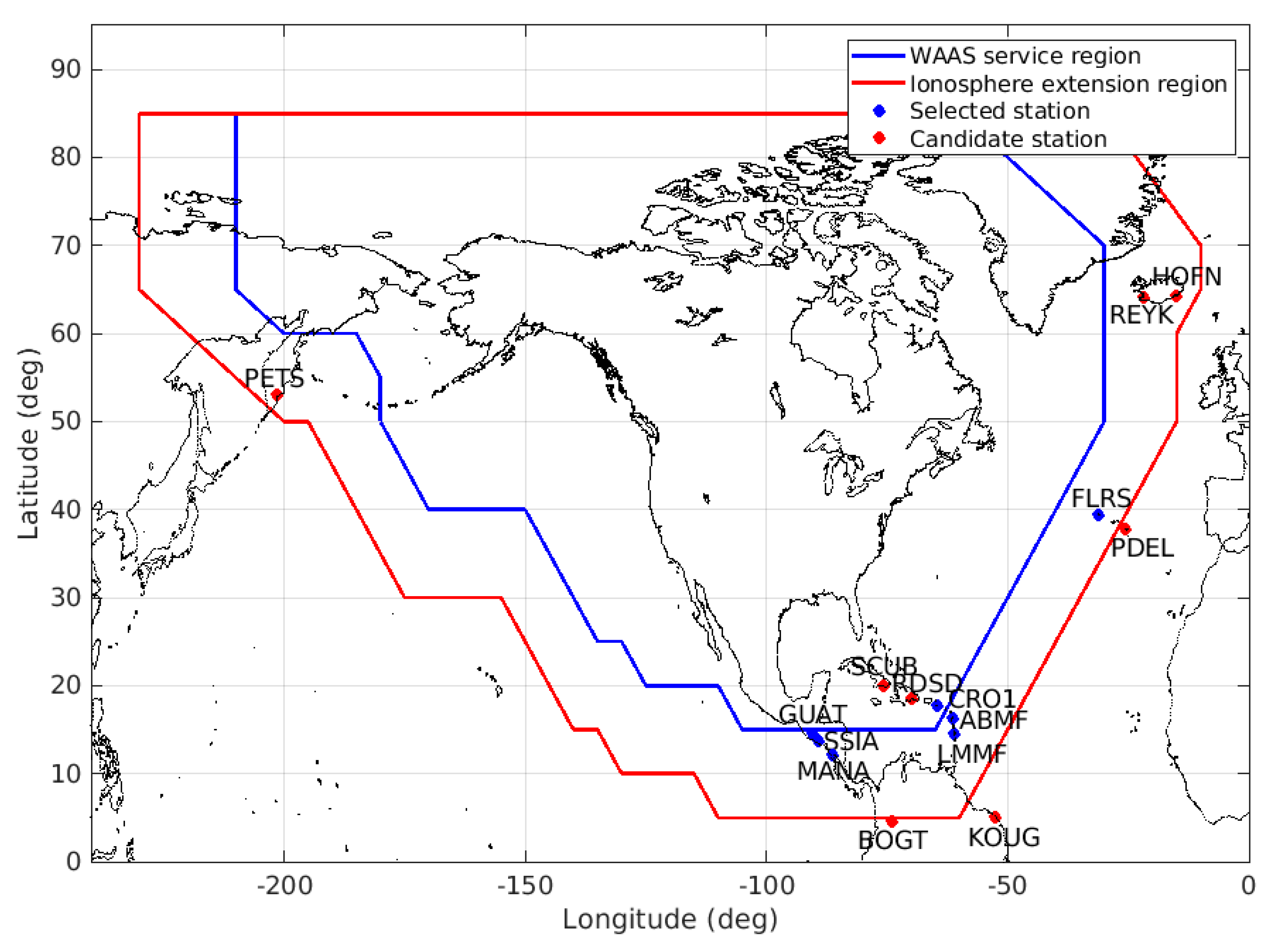
The ionosphere map extension algorithm was tested with US WAAS data. The WAAS was selected because it provides a stable ionosphere map with high availability [26,27]. WAAS ionospheric correction and its covariance were extended using the biharmonic spline technique with a preset extension area. The preset extension area along with the WAAS service area is shown in Figure 1. Fifteen international GNSS service (IGS) stations in the extension area were considered for performance evaluation and their locations are shown in Figure 1. The choice of the GNSS stations will be discussed later in Section 3.1. The original WAAS service area was extended to 15° in the east/west direction. The southern region, where the ionospheric variation is large, has a relatively worse extrapolation performance than the east/west direction, so it was only expanded up to 10° [16,17].
The ionospheric delay covariance, GIVE, was also extrapolated by using the biharmonic spline. At some points, the extrapolated GIVE values may have been out of range, greater than 15 or smaller than 0. Because a GIVE value of 15 represents inaccurate ionosphere information, any such data should be excluded from the extrapolation process. Accordingly, the maximum GIVE in the extrapolated region was set to 14. The extrapolated covariance should be greater than the original covariance because the extrapolated value should be less accurate than the original. For this reason, the minimum GIVE in the extrapolated region was set to 6. The value of 6 originated from the analysis of the WAAS GIVE values. At the WAAS center area, where the ionosphere correction is most accurate, the GIVE value is usually 6.
2.3.2. Positioning Algorithm
In order to evaluate the effect of the extended ionospheric delays, standard GNSS least-squares positioning was performed by using pseudorange code ranges and SBAS corrections. At the boundary of the SBAS service area, partial SBAS corrections were unavailable, especially ionosphere corrections. However, fast, orbit, and clock corrections are usually available even at the boundary. If the ionosphere correction is available for more than four satellites per epoch, PA mode is enabled. This study covered only the NPA mode when the number of ionosphere corrections was less than four. The NPA mode computes positions with the GPS ionosphere model (Klobuchar) and SBAS orbit/clock corrections. The NPA mode does not mix SBAS ionosphere corrections and the Klobuchar model. A bias exists between SBAS ionosphere corrections and the Klobuchar model, and as a result mixed use of them generally degrades positioning performance. This study used original and extended SBAS ionosphere corrections instead of the Klobuchar model when the number of ionosphere corrections was less than four.
Table 1 summarizes the positioning methods used in this study. Case 2 represents the original NPA positioning mode and Case 3 represents the enhanced NPA mode with the extended SBAS corrections. Case 1 represents the standard GPS only positioning mode that uses GPS broadcasted orbit, clock, and ionosphere models.
Figure 2 illustrates the IPPs of GPS satellites visible at MANA station at certain epochs. A total of 11 satellites were visible and three (No. 1–3) satellites’ IPPs were inside the SBAS (WAAS) service area. Seven (No. 4–10) satellites’ IPPs were in the extension area while one (No. 11) satellite’s IPP was outside the extension area. Case 2 used all (No. 1–11) satellites’ ranges for positioning but used Klobuchar for all the satellites. Case 3 used 10 satellites except for No. 11 satellite. The original SBAS ionosphere corrections were used for satellites No. 1–3 and extended ionosphere corrections were used for satellites No. 4–10. Case 1 used all 11 satellites’ ranges with broadcast orbit/clock and Klobuchar models.
3. Results
3.1. SBAS Ionospheric Correction Availability
In order to determine the WAAS ionosphere extension region, the availability of the WAAS ionosphere correction was analyzed. The ionosphere correction at a specific IGP is valid if its GIVE index is less than 15. The availability was analyzed with one month of SBAS data from March 2015. This period was selected because a large-scale ionosphere storm occurred, the St. Patrick’s Day storm on March 17, and ionospheric delay and variation were relatively high. Another one-month SBAS data from September 2013 was also analyzed for comparative study purposes. Both periods had large solar and geomagnetic indices and caused large ionosphere delays. Since the proposed method improves ionospheric delay accuracy, a period of high solar activity is suitable for performance evaluation analysis.
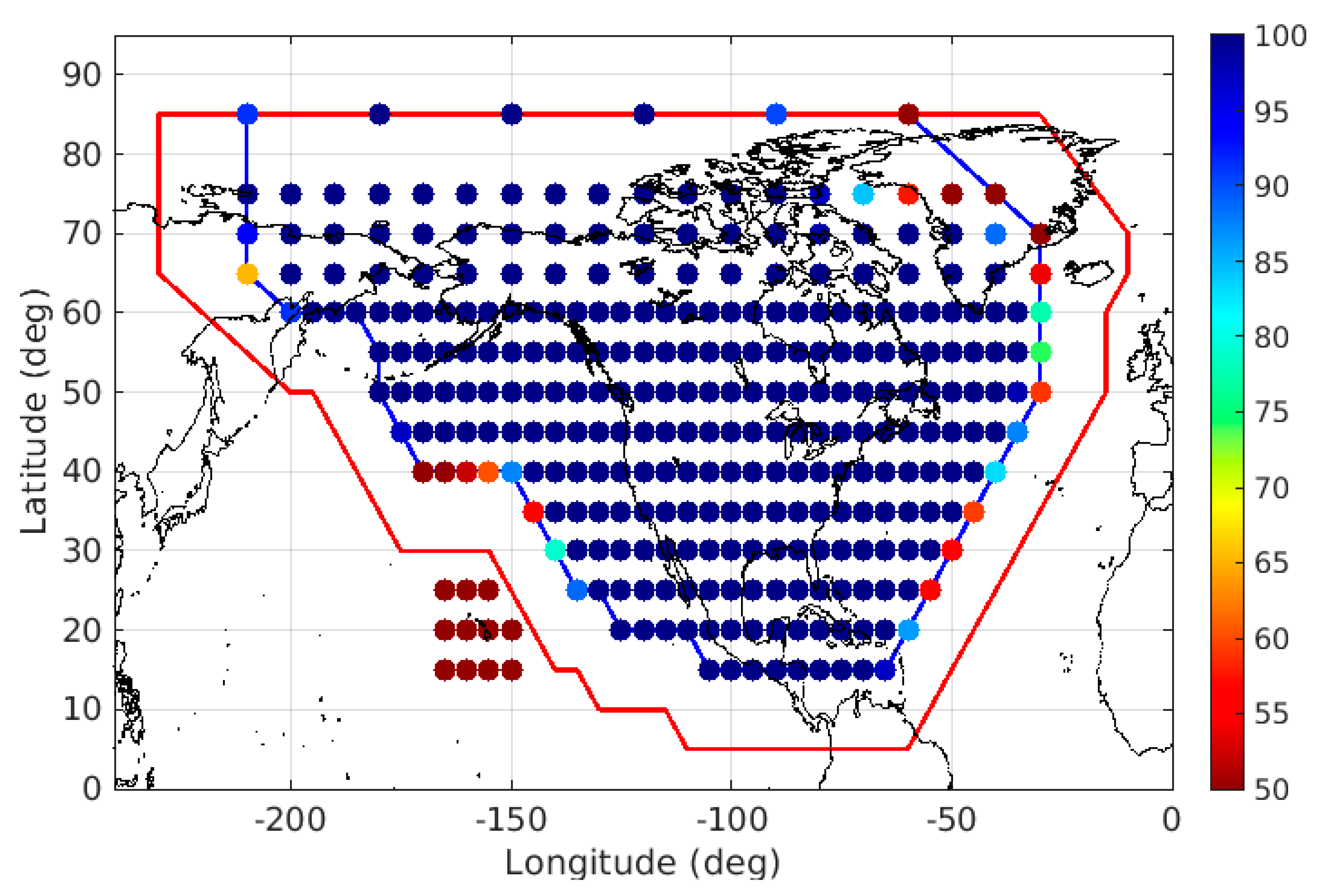
Figure 3 shows the availability of WAAS ionosphere corrections in March 2015. One month of availability data was averaged at each IGP. Other corrections, FC and LTC, were not considered because they usually have better availability than the ionosphere correction. The ionosphere correction availability was close to 100% in most of the WAAS service area except boundary points. On the east and west boundary points, the availability dropped rapidly and was nearly 50%. When comparing the distance from WAAS ground stations, the east and west boundaries were farther than the southern boundary.
For the performance evaluation of the proposed method, we considered 15 IGS stations in the ionosphere extension region. The locations of those stations are shown in Figure 1. Because the east and west side of the WAAS service area is the sea, there were few IGS stations in the extended area, and most of them were in the south area. Ionosphere extension does not imply an extended service area. It represents the area where the extended ionosphere corrections are provided for a GNSS satellite, whose IPP is inside the extension area. For this reason, the feasible extension area was smaller than the ionosphere extension area. Prior to the stations’ selection process, the WAAS signal availability was analyzed at the candidate stations. GPS observations at those stations were used to find visible satellites, whose PRN was compared with the PRN in WAAS corrections to check if the WAAS correction was available for a specific satellite.
Table 2 summarizes the SBAS correction availability of the fifteen stations in March 2015. The SBAS orbit/clock correction ratio was computed by dividing the number of SBAS orbit/clock corrections in one month by the total number of satellite range observations in one month. The SBAS ionosphere correction ratio was computed in the same way. The fifth column represents the PA availability that was computed by the following method. At every 30s, the number of full SBAS correction satellites (both orbit/clock and ionosphere corrections available) was divided by the total number of satellite range observations. The PA availability was the one month mean of those ratios. The NPA/GPS availability was computed in the same way. This is why the PA availability was different from the ionosphere correction ratio. At the SSIA station, the full SBAS correction was available for 69.4% of the period, and the NPA mode computation was performed for the remaining 30.6%. No GPS only positioning mode (0%) implies more than three orbit/clock corrections are available all the time. At FLRS station, only 1.4% of the period provided the full SBAS corrections, therefore, the NPA mode positioning should be performed during the remaining 98.6% of the period.
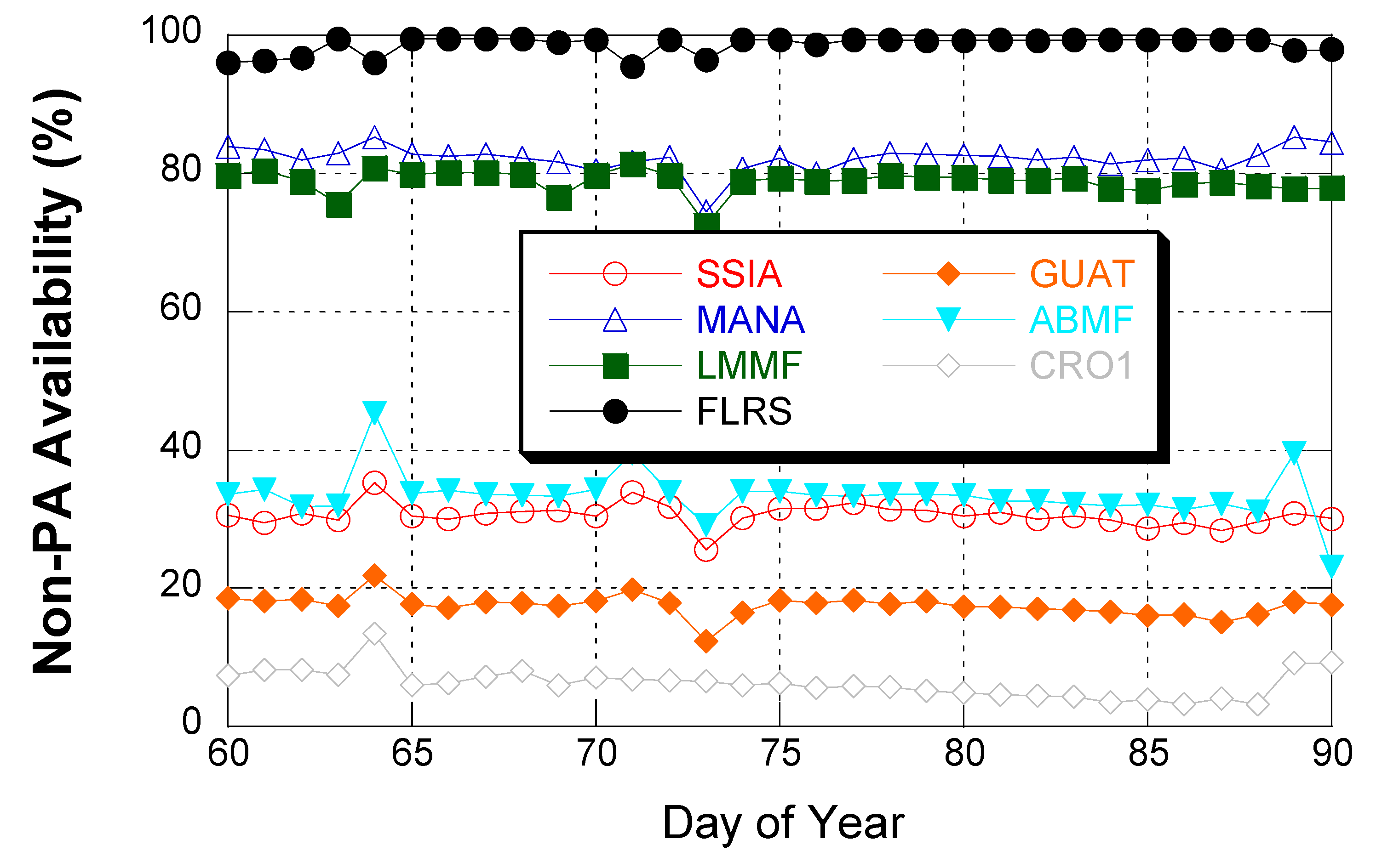
Two stations, SCUB and RSDS, have 100% PA mode availability and do not require the proposed method of improving NPA mode availability. The proposed method mixes the original and extended SBAS ionosphere corrections, and the GNSS station location with partial SBAS ionospheric correction is suitable for applying the proposed method. For this reason, five stations, PDEL, HOFN, BOGT, KOUG, and PETS, were excluded because they had 0% PA mode availability. Another exclusion was the REYK station with 92.7% NPA availability. Preliminary experiments with REYK showed little improvement in accuracy with extended ionosphere corrections. This was because the ionospheric delay at the high latitude was so small that the ionospheric delay did not lead to a significant improvement in positioning accuracy. Another reason was that REYK’s latitude is very high and GPS satellites are not available in the polar regions, so the GPS observability is very low. Poor observability degrades GPS positioning accuracy and makes it difficult to assess the effect of ionosphere delay. After the screening process, seven stations, SSIA, MANA, LMMF, FLRS, GUAT, ABMF, and CRO1, were selected for GPS positioning accuracy evaluation. CRO1 was inside the WAAS service area and had very low NPA mode availability (5.0%). CRO1 may not have had significant benefits with the ionosphere extension method. However, CRO1 was included in the evaluation for comparative study purposes.
Figure 4 shows the NPA availability variation of seven selected stations in March 2015. The NPA availability was computed at each station on a daily basis. The one month mean of these values corresponds to the sixth column of Table 2. SSIA and MANA are close to each other but their PA/NPA availabilities were very different. At the boundary of the SBAS service area, a small distance change caused a large availability change. Another cause of the availability difference was the two stations’ observability difference. MANA station has a lower observability condition than SSIA does due to a wall in the west direction [28], which blocks GPS signals with a low elevation angle below 10 degrees in the west direction. The signal loss was identified by inspecting observation data at the MANA station. MANA station’s signal loss reduced its PA availability.
3.2. Ionospheric Delay Errors
The accuracy of the extended WAAS ionosphere corrections was evaluated with the one month of SBAS data in March 2015. IGS provides the global ionosphere model (GIM) by using IGS monitoring station data. Because IGS utilizes a large number of GNSS monitoring station data with a post-processing algorithm, IGS GIM should be more accurate than SBAS real-time processing, and thus was selected as a truth ionosphere for the accuracy evaluation. The difference between WAAS and IGS GIM ionospheric delays was calculated at the extended ionosphere map area.
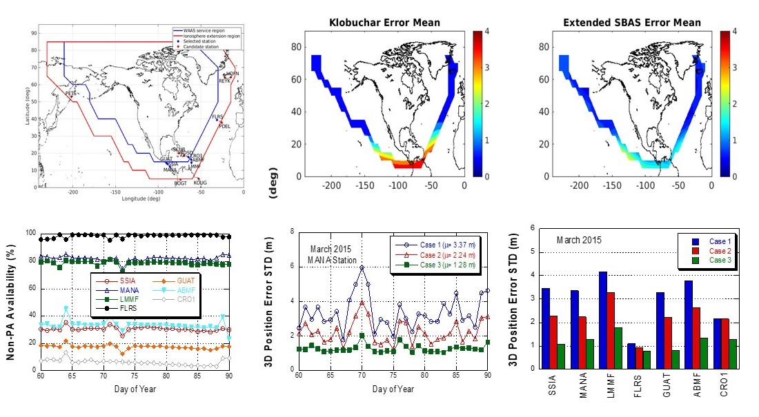
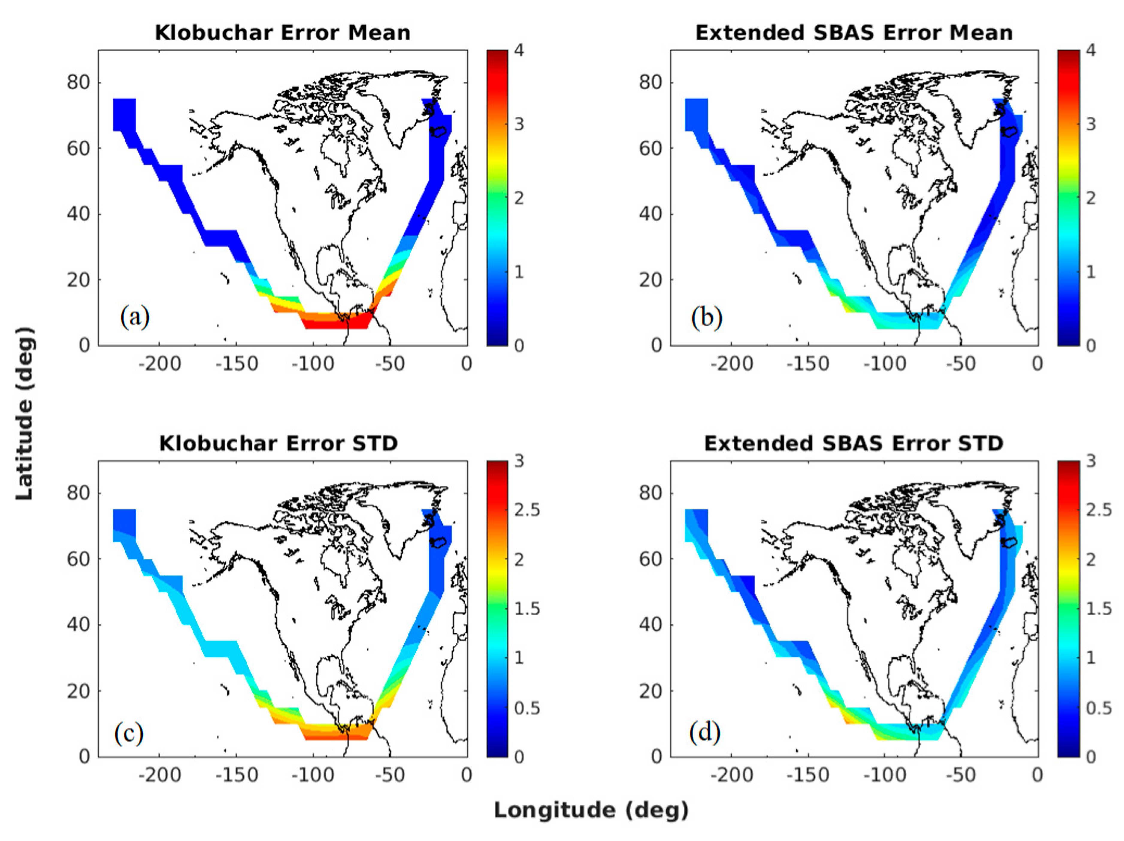
Figure 5 shows the mean and standard deviation of the extended SBAS ionosphere correction errors in the extension region. Ionospheric delay error statistics by GPS Klobuchar are presented for comparison. With one month of SBAS data, the ionospheric delay error was computed at each IGP point by subtracting the extended SBAS ionospheric delay from the IGS GIM ionospheric delay. The mean values of Figure 5a,b represent the absolute mean of the errors. The mean error level of extended SBAS ionosphere correction was far lower than that of the Klobuchar model, especially in low latitudes below 20°. The mean error reduction by the extended correction over the Klobuchar model was 23.4% but the reduction at low latitudes below 20° was 52.3%. In the high latitude, the magnitude of ionospheric delay itself was low and the accuracy improvement by the extended SBAS ionosphere correction was not significant. Similar accuracy improvement by the extended SBAS was shown in the error STD of Figure 5c,d. As well as the ionosphere error magnitude, the error variation was reduced by using the extended corrections. This period, March 2015, had a high ionospheric delay, and the Klobuchar model value was usually lower than the actual ionospheric delay value [26].
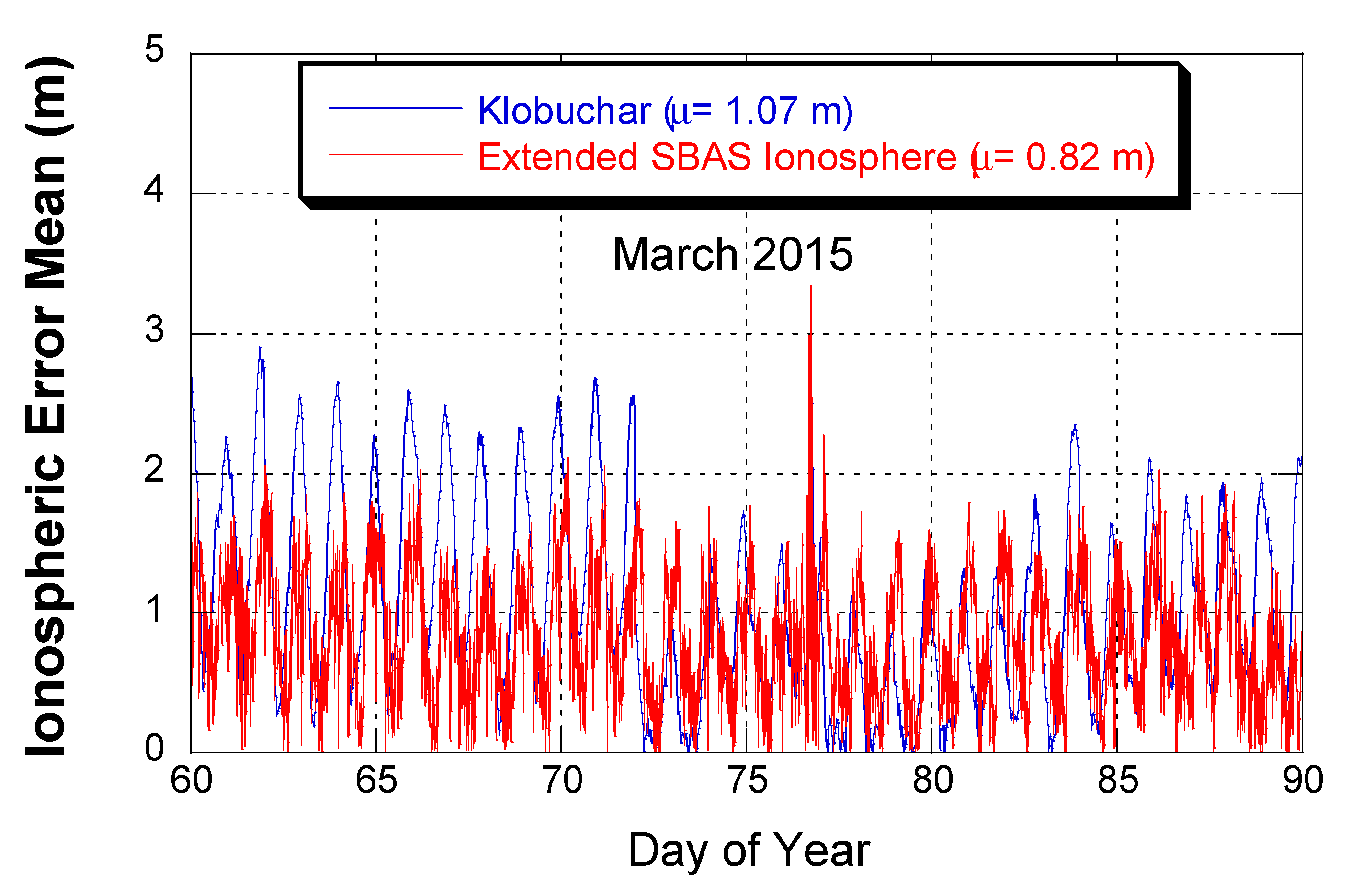
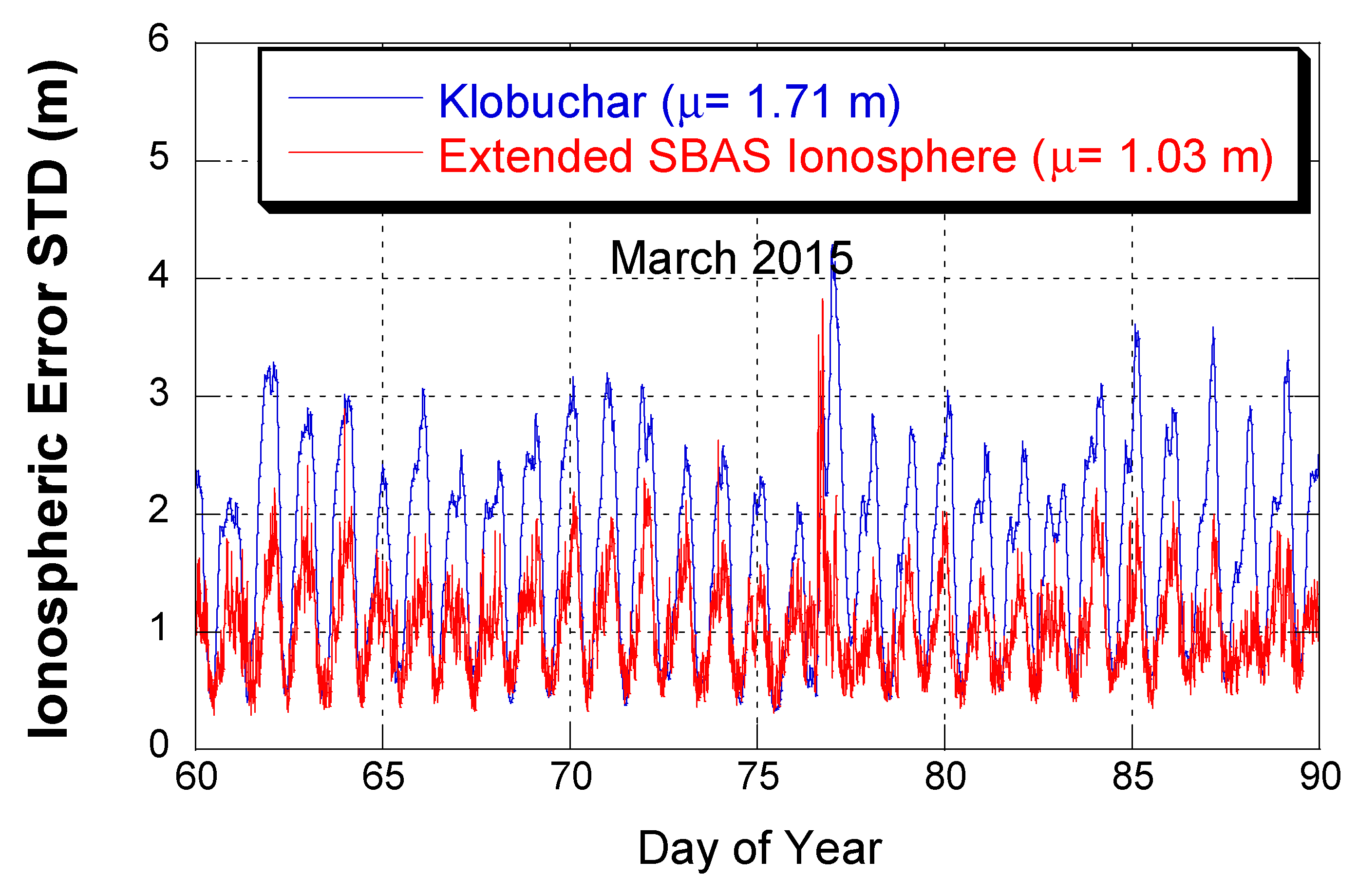
Figure 6 and Figure 7 show the time series of ionospheric error mean and STD in March 2015. The ionospheric delay errors at the extended IGPs were averaged for each epoch, every 300s seconds. From Figure 6, it is clear that the SBAS extrapolation reduced the ionosphere errors; the error mean was reduced by 23.4%. Reduction of the error STD was more significant, at 39.8%. Therefore, the use of the SBAS extended ionosphere was more effective in reducing error STD than in reducing error mean. Most of the error reduction occurred during the daytime when the ionospheric delay level was high. The maximum error was observed on March 17 when the St. Patrick’s Day ionosphere storm occurred. During this storm period, the error mean of the SBAS extension was similar to that of Klobuchar, but the error STD of the SBAS extension was lower than that of Klobuchar.
Additional experiments with the Galileo NeQuick-G model were performed. While NeQuick is not currently used for SBASs, it offers better performance than Klobuchar in general. NeQuick’s level of accuracy is between Klobuchar and SBAS. On 14 March 2015, the mean of the ionospheric delay errors weas 1.01 m (Klobuchar), 0.97 m (NeQuick), and 0.81 m (SBAS), respectively. The STD of the ionospheric delay errors were 1.44 m (Klobuchar), 1.21 m (NeQuick), and 0.99 m (SBAS), respectively. The performance improvement from NeQuick over Klobuchar was significant at low latitudes.
3.3. Positioning Errors
Positioning accuracy improvement with the extended SBAS ionosphere correction was evaluated. SBAS aided-GPS standard positioning with L1 code pseudoranges observed at seven selected stations was performed. Weighted least square estimation, the same as the SBAS positioning, was used. Three types of positioning methods described in Table 1 were evaluated. IGS GPS observations were used and the positioning interval was 30s.
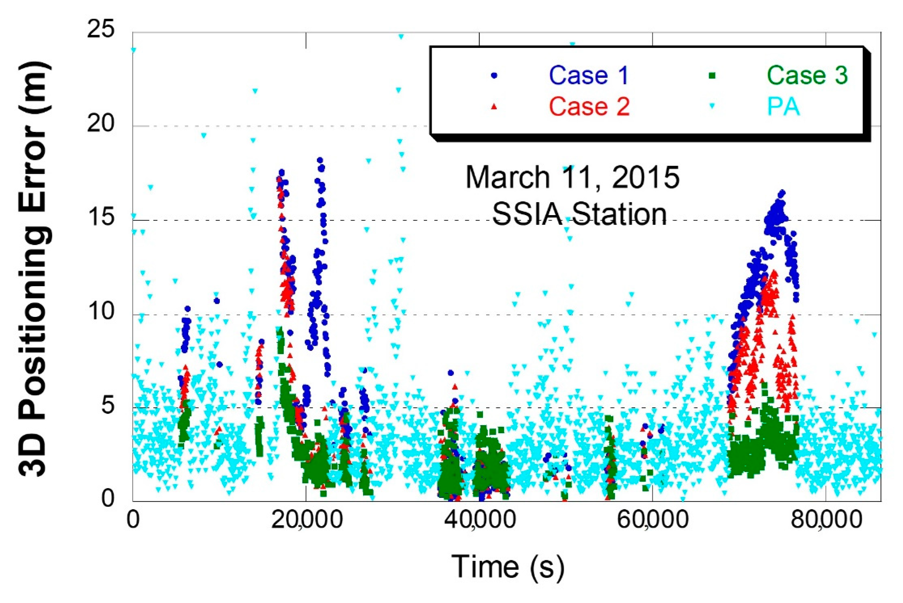
Figure 8 shows the position error time series at the SSIA station on 11 March 2015. The SBAS positioning mode selection depends on the availability of SBAS ionosphere correction. When four or more satellites could use all the SBAS corrections, both orbit/clock and ionosphere, PA mode positioning was used. Otherwise, the three positioning modes of Cases 1, 2, and 3 were used. The later cases still used orbit/clock corrections. The PA mode availability was 69.4% on this date. In some instances, PA mode had a large error, usually when only four satellite measurements were used. This plot clearly showed the accuracy improvement by the SBAS orbit/clock corrections (Cases 2 and 3) over GPS broadcast orbit/clock (Case 1). The extended ionosphere correction of Case 3 improved the accuracy especially during the large positioning error period around 20,000 s and 72,000 s. The improvement in positioning accuracy was not observed between 30,000 s and 60,000 s, since the time range corresponded to the night time of the SSIA station (UTC -6 h). In other words, the improvement in positioning accuracy was not significant when the ionospheric delay was small.
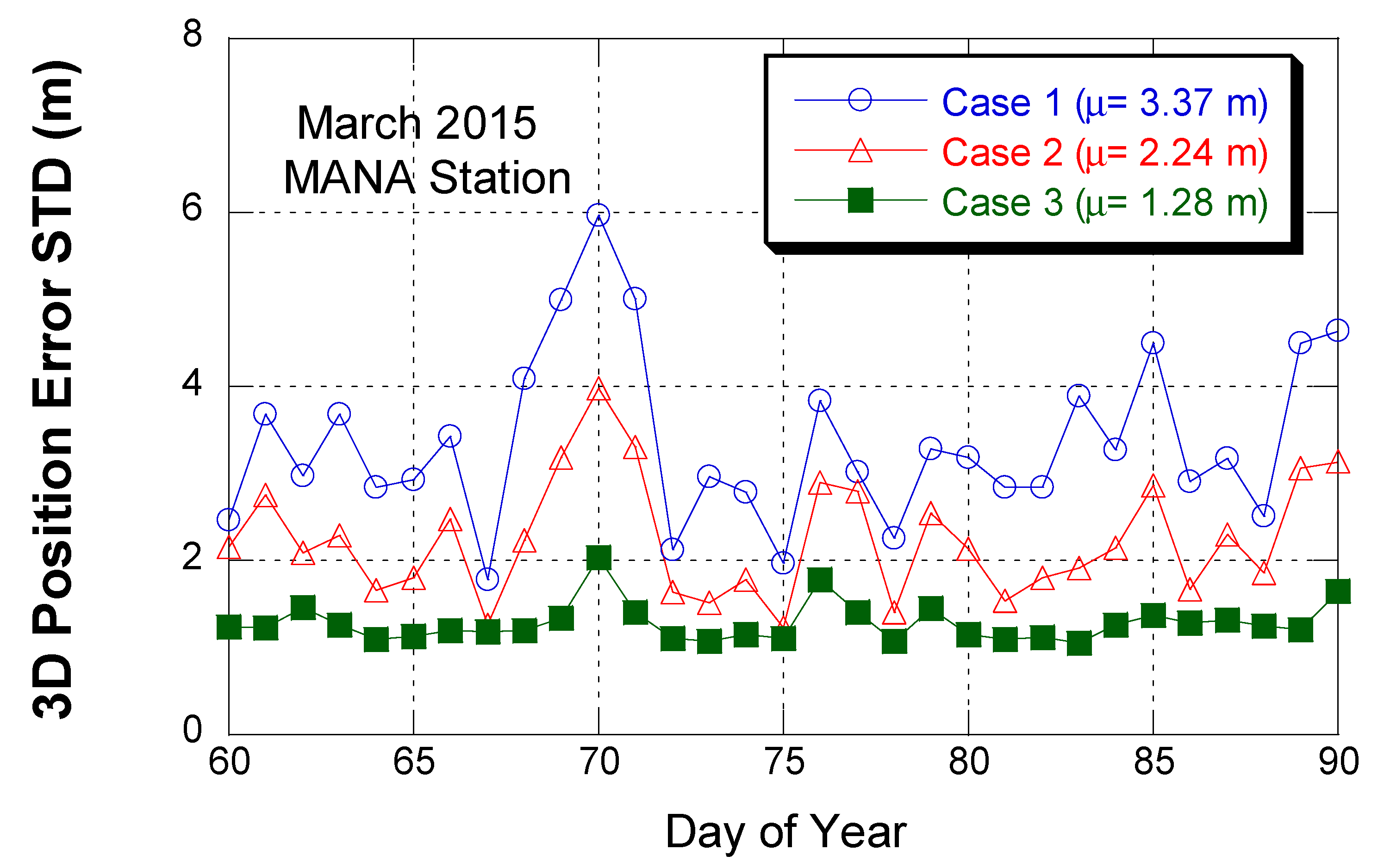
Figure 9 shows the variation of the position error STD at MANA station in March 2015. Daily positioning error STD was computed for the NPA period, which accounted for 84.4% of all data periods. As seen above, cases 1 and 2 had a large variation but Case 2 had a lower magnitude. However, Case 3 had a much lower variation than Cases 1 and 2, and it established the ionospheric delay error was a dominant error source in single-frequency GNSS positioning.
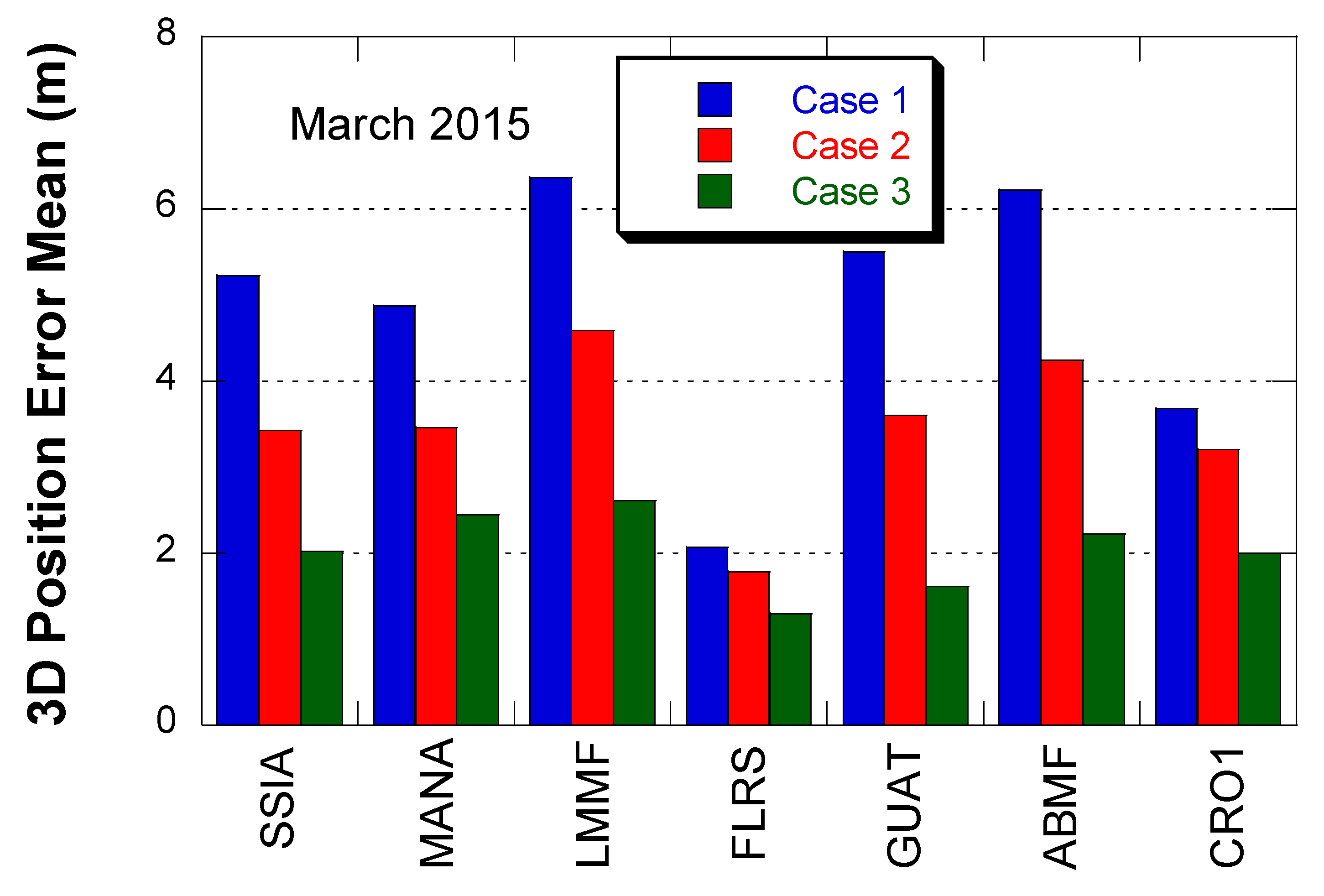
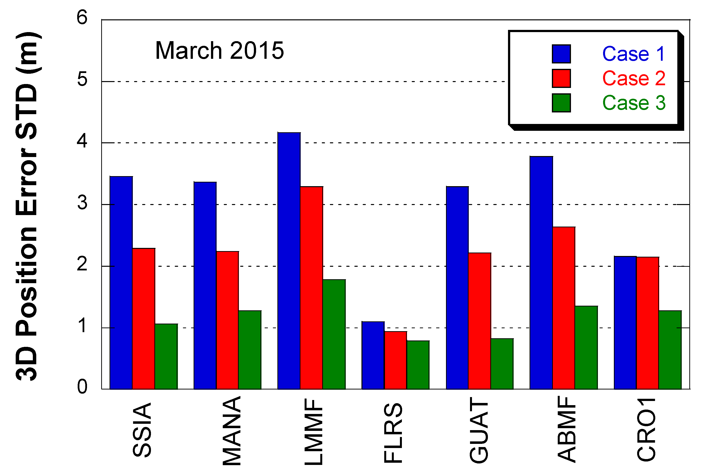
Figure 10 and Figure 11 show the mean and STD of 3D positioning error with one month of data in March 2015. The error statistics were computed for NPA mode. For example, as shown in Table 2, 69.4% of SSIA station positioning results were obtained by PA mode and 30.6% of the positioning results were used for the error statistics of Figure 10 and Figure 11. Both the mean and STD statistics showed a clear error reduction by using the extended ionosphere corrections. The positioning error reduction from Case 2 to 3 was 41.1% in mean and 46.84% in STD. The positioning error level at FLRS was relatively lower than the six other stations due to the low ionospheric delay at high latitude. The distance from the SBAS service area boundary to the GNSS stations can influence the improvement in positioning accuracy by the extension method. However, the accuracy correlation with distance was not clear in these experiments. This was because the ionospheric delay levels and correction accuracies were different for each station. When more GNSS stations are available, the effect of the distance can be analyzed.
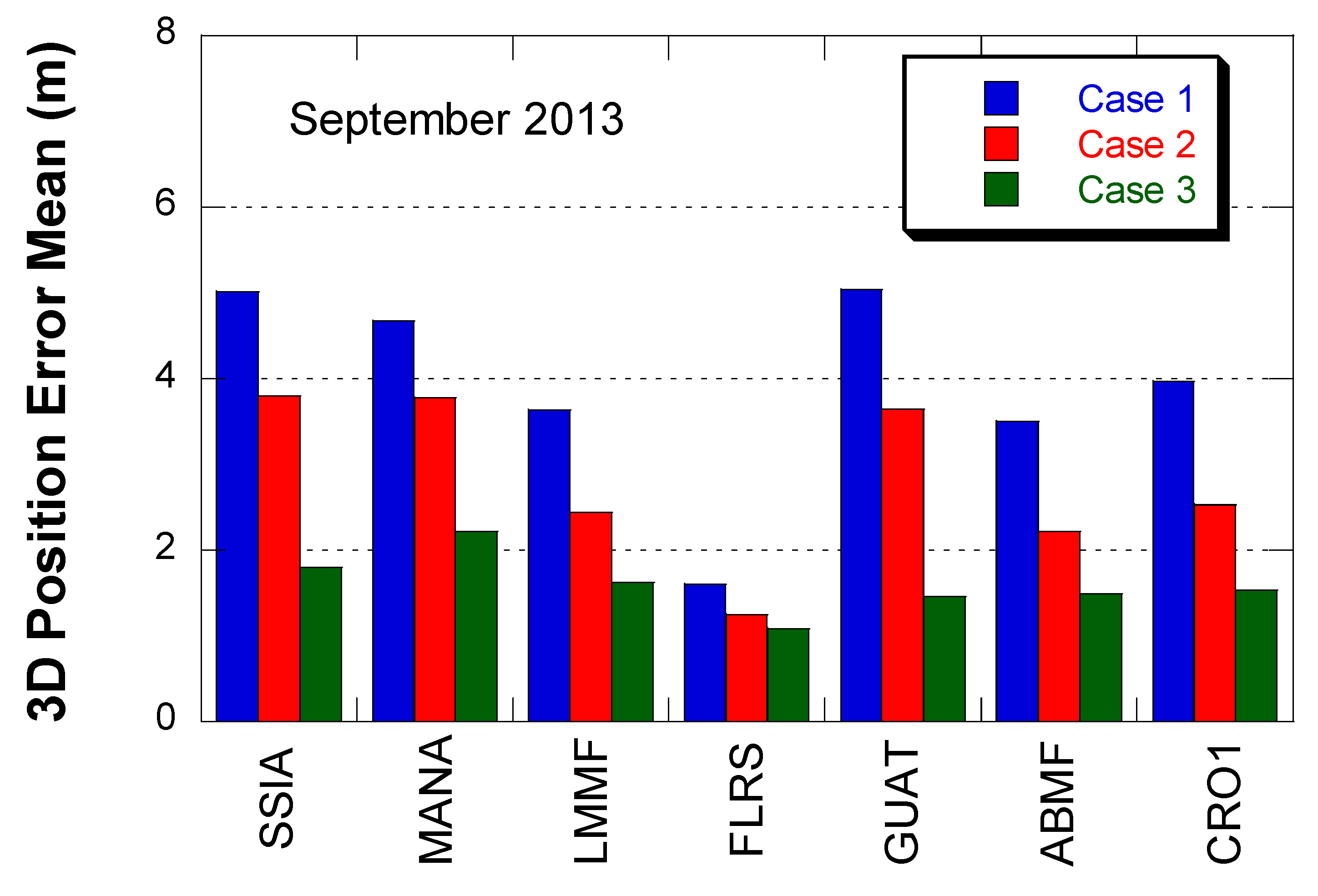
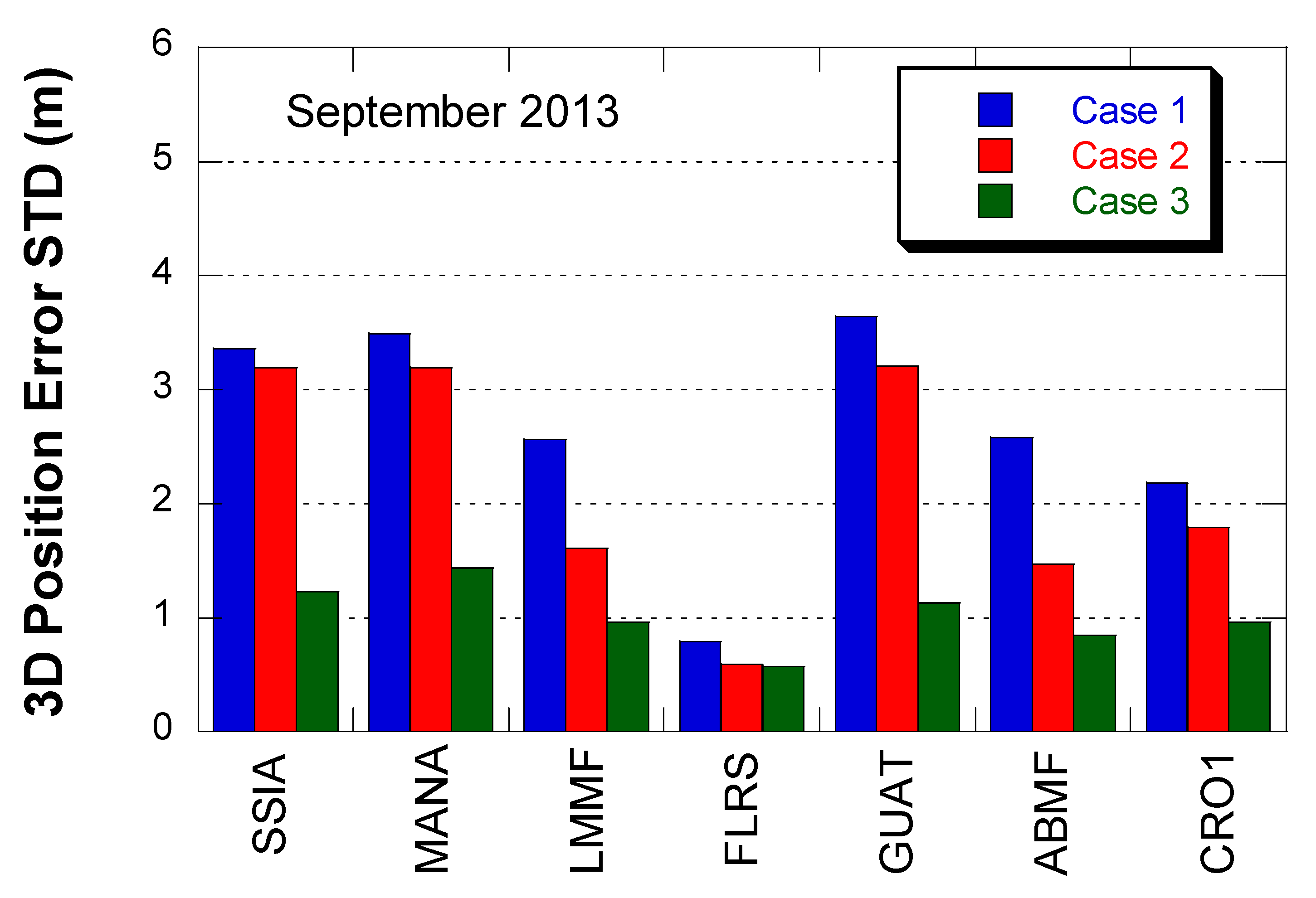
Figure 12 and Figure 13 show the mean and STD of 3D positioning error with one month of data in September 2013. The overall error level was slightly lower than the March 2015 results, but the error reduction from Case 2 to 3 was still significant. The positioning error reduction from Case 2 to 3 was 43.0% in mean and 52.6% in STD. CRO1 is inside the WAAS service area but showed a similar error reduction.
The horizontal and vertical positioning error statistics in March 2015 are shown in Table 3 and Table 4. In general, the ionospheric delay affected vertical positioning error more than horizontal positioning error because the ionospheric delay was parallel to the pseudorange signal and its mean direction was the zenith direction. It implied that the ionosphere correction effect was more significant in the vertical positioning accuracy than in the horizontal positioning accuracy. The error reduction magnitude of the vertical error, both in mean and STD, was greater than that of the horizontal error. But there was no significant difference between the horizontal and vertical error reduction ratio. Shown in Figure 10 and Figure 11, the error level and error reduction were not as significant at FLRS as it was at the three other stations. If we looked at the statistics of the six stations, except FLRS, one-month averages of the error reduction from Case 2 to Case 3 were 44.8% (horizontal mean), 45.5% (vertical mean), 44.1% (horizontal STD), and 43.1% (vertical STD).
Table 5 and Table 6 show the positioning error statistics in September 2013. Their overall error reduction trend was similar to the 2015 results. If we looked at the statistics of the six stations at the south area excluding FLRS, one-month averages of the error reduction from Case 2 to Case 3 were 45.5% (horizontal mean), 45.5% (vertical mean), 44.9% (horizontal STD), and 47.4% (vertical STD). The reduction ratio was slightly higher than the ratio of 2015.
4. Discussion
Experimental results show a significant reduction in positioning errors using the SBAS ionosphere extension method. This method is effective when the ionospheric delay is large. Therefore, the error reduction is more significant at lower latitudes than higher latitudes. It is also effective during a high solar activity period because the ionospheric delay is large. The southern boundary of the WAAS service area has high ionospheric delays and large fluctuations in delay. Using a local ionospheric model, such as SBAS, can reduce the impact of the ionospheric delay error, and the proposed method can help.
At 39.45° N latitudes, the FLRS station’s positioning accuracy is rarely improved because a small ionosphere delay occurs at that latitude. Another reason for error reduction is that it is far from the WAAS service area boundary. FLRS is relatively farther from the border than other stations. This difference in distance results in a significant difference in PA mode availability, and the PA mode ratio of FLRS is very low at 1.4%. This means that the number of original SBAS ionospheric corrections per epoch is less than four most of the time. A small number of original SBAS ionospheric corrections imply a small number of extended SBAS ionospheric corrections. The proposed ionospheric expansion method uses only the original or extended SBAS correction and does not use the Klobuchar model outside the extended region. Therefore, the number of GPS satellites used for the positioning is relatively small at FLRS, close to the minimum number of four. Using a small number of GPS signals results in poor positioning performance regardless of ionospheric delay correction.
The current implementation of the extrapolation algorithm is the biharmonic spline interpolation. With a simple formula, the biharmonic method is suitable for GNSS-SBAS receiver embedded code. Using more sophisticated extrapolation algorithms, e.g., machine learning, ionospheric extrapolation accuracy can be significantly improved. However, for real-time processing, considerable corrections are required. Modifying the extrapolation process in addition to the extrapolation algorithm itself helps improve ionospheric correction accuracy. For example, the current implementation uses the same algorithm for the south and other directions. The ionospheric delay magnitude is quite different in the south direction and the other direction, so some type of algorithm modification, e.g., different weights in each direction, can help to increase accuracy.
The biharmonic spline interpolation algorithm does not use the ionospheric delay feature at all. There is no information about the ionosphere properties or spatial environment. Recent advances in the effect of ionospheric delays on GNSS carrier frequencies can be considered for further study. For example, Kuverova et al. [29] showed that the Rydberg complex is a major cause of the ionospheric delay in GPS signals. In the radio occultation experiments, scintillation observation confirms this effect [30]. The information from these new ionospheric studies can help improve ionospheric extension algorithms and ionospheric correction accuracy.
SBAS is designed to improve standard point positioning (SPP) accuracy by using code pseudo ranges rather than precise point positioning (PPP) by using carrier phases. While SBAS’s overall level of accuracy is considerably lower than that of PPP, SBAS provides integrity information for consistent and reliable positioning. It is not worth comparing SBAS accuracy with PPP accuracy. SBAS positioning process is quite different from the PPP positioning process due to handling of SBAS integrity information. Applying the proposed algorithm to PPP can be a topic of further research.
5. Conclusions
SBAS provides correction information for improving GNSS positioning accuracy and integrity. The correction includes satellite orbit, clock, and ionospheric delay information. Near the boundary of the SBAS service area, the correction is not fully available and only a partial correction is available, mostly derived from satellite orbit and clock information. In this case, the GNSS ionosphere model, e.g., GPS Klobuchar, replaces the ionosphere corrections. By using the geospatial correlation property of the ionosphere delay information that is provided at predefined geographic locations, the ionosphere correction coverage can be extended by a spatial extrapolation algorithm.
In this research, the WAAS ionosphere map was extended by a biharmonic extrapolation algorithm. It is a simple algorithm that can be easily implemented in GNSS receivers. GPS positioning accuracy was evaluated at seven IGS stations in the vicinity of the WAAS service area. In addition to the ionospheric delay information, ionospheric delay estimation covariance was extrapolated for determining measurement weightings during the positioning process. The SBAS protection level, error bound of position error estimates, was not computed in this research.
Ionospheric delay accuracy in the extended service area was compared with the Klobuchar model. Since in general the ionosphere accuracy improvement by the extended ionosphere was proportional to ionosphere delay magnitude, the accuracy improvement over Klobuchar was significant in low latitude area, below 35° N. The extended ionosphere correction reduced both the mean and STD of the error. The absolute mean reduction of the ionosphere error below latitude 50° was 42.8%.
GPS positioning accuracy in the extended service area was evaluated with three methods; GPS only (Case 1), SBAS orbit/clock correction plus Klobuchar model (Case 2), and SBAS orbit/clock plus extended ionosphere corrections (Case 3). The GPS standard positioning with code pseudoranges and SBAS corrections was performed. Positioning error reduction was clear from Case 2 to Case 3, both in horizontal and vertical directions. 41.1% and 46.84% reductions were observed in 3D positioning error mean and STD, respectively. Due to the large ionospheric delays at low latitude, the positioning error reduction by the extended ionosphere correction was significant in the low latitude.
Author Contributions
Conceptualization, J.K.; Funding acquisition, J.K.; Project administration, J.K.; Software, M.K.; Supervision, J.K.; Validation, M.K.; Visualization, M.K.; Writing—Original draft, M.K.; Writing—Review & editing, J.K. All authors have read and agreed to the published version of the manuscript.
Funding
This research was supported by Basic Science Program funded by the Ministry of Science and ICT (NRF-2019R1F1A1062605).
Institutional Review Board Statement
Not applicable.
Informed Consent Statement
Not applicable.
Data Availability Statement
Not applicable.
Conflicts of Interest
The authors declare no conflict of interest.
References
- Kumluca, A.; Tulunay, E.; Topalli, I. Temporal and spatial forecasting of ionospheric critical frequency using neural networks. Radiol. Sci. 1999, 34, 1497–1506. [Google Scholar] [CrossRef]
- McKinnell, L.A.; Friedrich, M. A neural network-based ionospheric model for the auroral zone. J. Atmos. Sol. Terr. Phys. 2007, 69, 1459–1470. [Google Scholar] [CrossRef]
- Huang, Z.; Yuan, H. Ionospheric single-station TEC short-term forecast using RBF neural network. Radiol. Sci. 2014, 49, 283–292. [Google Scholar] [CrossRef]
- Jayapal, V.; Zain, A.F.M. Interpolation and extrapolation techniques based neural network in estimating the missing ionospheric TEC data. In Proceedings of the Progress in Electromagnetic Research Symposium (PIERS), Shanghai, China, 8–11 August 2016; pp. 695–699. [Google Scholar]
- Razin, M.R.G.; Voosoghi, B. Wavelet neural networks using particle swarm optimization training in modeling regional ionospheric total electron content. J. Atmos. Sol. Terr. Phys. 2016, 149, 21–30. [Google Scholar] [CrossRef]
- Chen, C.; Wu, Z.S.; Ban, P.P.; Sun, S.J.; Xu, Z.W.; Zhao, Z.W. Diurnal specification of the ionospheric f0F2 parameter using a support vector machine. Radiol. Sci. 2010, 45, 1–13. [Google Scholar] [CrossRef]
- Akhoondzadeh, M. Support vector machines for TEC seismo-ionospheric anomalies detection. Ann. Geophys. 2013, 31, 173–186. [Google Scholar] [CrossRef] [Green Version]
- Orús, R.; Hernández-Pajares, M.; Juan, J.M.; Sanz, J. Improvement of global ionospheric VTEC maps by using kriging interpolation technique. J. Atmos. Sol. Terr. Phys. 2005, 67, 1598–1609. [Google Scholar] [CrossRef]
- Wielgosz, P.; Grejner-Brzezinska, D.; Kashani, I. Regional ionosphere mapping with kriging and multiquadric methods. J. Glob. Position. Syst. 2003, 2, 48–55. [Google Scholar] [CrossRef]
- Foster, M.P.; Evans, A.N. An Evaluation of Interpolation Techniques for Reconstructing Ionospheric TEC Maps. IEEE Trans. Geosci. Remote Sens. 2008, 46, 2153–2164. [Google Scholar] [CrossRef]
- Ogryzek, M.; Krypiak-Gregorczyk, A.; Wielgosz, P. Optimal geostatistical methods for interpolation of the ionosphere: A case study on the St. Patrick’s Day storm of 2015. Sensors 2020, 20, 2840. [Google Scholar] [CrossRef]
- Leandro, R.F.; Santos, M.C. A neural network approach for regional vertical total electron content modelling. Stud. Geophys. Geod. 2006, 51, 279–292. [Google Scholar] [CrossRef]
- Habarulema, J.B.; McKinnell, L.A.; Opperman, B.D.L. Regional GPS TEC modeling; Attempted spatial and temporal extrapolation of TEC using neural networks. J. Geophys. Res. 2011, 116, 1–14. [Google Scholar] [CrossRef]
- Okoh, D.; Owolabi, O.; Ekechukwu, C.; Folarin, O.; Arhiwo, G.; Agbo, J.; Bolaji, S.; Rabiu, B.A. Regional GNSS-VTEC model over Nigeria using neural networks: A novel approach. Geod. Geodyn. 2016, 7, 19–31. [Google Scholar] [CrossRef] [Green Version]
- Kim, J.; Kim, M. Extending ionospheric correction coverage area by using extrapolation methods. J. Korean Soc. Aviat. Aeronaut. 2014, 22, 74–81. [Google Scholar] [CrossRef] [Green Version]
- Kim, M.; Kim, J. Extending ionospheric correction coverage area by using a neural network method. Int. J. Aeronaut. Space Sci. 2016, 17, 64–72. [Google Scholar] [CrossRef] [Green Version]
- Kim, M.; Kim, J. Extending the coverage area of regional ionosphere maps using a support vector machine algorithm. Ann. Geophys. 2019, 37, 77–87. [Google Scholar] [CrossRef] [Green Version]
- Ryu, G.D.; So, H.; Park, H.W. Performance analysis of artificial neural network for expanding the ionospheric correction coverage of GNSS. J. Adv. Navig. Technol. 2018, 22, 409–414. [Google Scholar] [CrossRef]
- RTCA. Minimum Operational Performance Standards for Global Positioning System/Wide Area Augmentation System Airborne Equipment, DO-229D; Radio Technical Commission for Aeronautics (RTCA): Washington, DC, USA, 2013. [Google Scholar]
- GNSS Tools Team. PEGASUS: Technical Notes on SBAS; PEG-TN-SBAS; Eurocontrol: Brussels, Belgium, 2003. [Google Scholar]
- FAA. WAAS Terms and Definitions Page. Available online: https://www.nstb.tc.faa.gov/DisplayDefinitions.htm (accessed on 3 November 2020).
- FAA. Wide-Area Augmentation System Performance Analysis Report; WAAS Performance Analysis Report; FAA: Washington, DC, USA, 2015.
- Klobuchar, J.A. Ionospheric time-delay algorithm for single-frequency GPS users. IEEE Trans. Aerosp. Electron. Syst. 1987, 23, 325–331. [Google Scholar] [CrossRef]
- Sandwell, D.T. Biharmonic spline interpolation of GEOS-3 and SEASAT altimeter data. Geophys. Res. Lett. 1987, 14, 139–142. [Google Scholar] [CrossRef] [Green Version]
- Feliciano-Cruz, L.I. Biharmonic spline interpolation for solar radiation mapping using Puerto Rico as a case of study. In Proceedings of the IEEE Photovoltaic Specialists Conference (PVSC), Austin, TX, USA, 3–8 June 2012; pp. 2913–2915. [Google Scholar]
- Kim, J.; Kim, M. NeQuick G model based scale factor determination for using SBAS ionosphere corrections at low earth orbit. Adv. Space Res. 2020, 65, 1414–1423. [Google Scholar] [CrossRef]
- Nie, Z.; Zhou, P.; Liu, F.; Wang, Z.; Gao, Y. Evaluation of orbit, clock, and ionospheric corrections from five currently available SBAS L1 service: Methodology and analysis. Remote Sens. 2019, 11, 411. [Google Scholar] [CrossRef] [Green Version]
- UNAVCO Station Page. Available online: https://www.unavco.org/instrumentation/networks/status/nota/photos/MANA (accessed on 30 November 2020).
- Kuverova, V.V.; Adamson, S.O.; Berlin, A.A.; Bychkov, V.L.; Dmitriev, A.V.; Dyakov, Y.A.; Eppelbaum, L.V.; Golubkov, G.V.; Lushnikov, A.A.; Manzhelii, M.I.; et al. Chemical physics of D and E layers of the ionosphere. Adv. Space Res. 2019, 64, 1876–1886. [Google Scholar] [CrossRef]
- Su, S.Y.; Tsai, L.C.; Liu, C.H.; Nayak, C.; Caton, R.; Groves, K. Ionospheric Es layer scintillation characteristics studied with Hilbert-Huang transform. Adv. Space Res. 2019, 64, 2137–2144. [Google Scholar] [CrossRef]
Figure 1.
WAAS service and extended regions with the location of selected and candidate international GNSS service (IGS) stations.
Figure 1.
WAAS service and extended regions with the location of selected and candidate international GNSS service (IGS) stations.

Figure 2.
GPS Satellite ionosphere pierce points (IPPs) visible at MANA station on 17 March 2015.

Figure 3.
One-month average of WAAS ionosphere correction availability in March 2015.

Figure 4.
Non-precision approach (NPA) availability variation at seven selected IGS stations in March 2015.
Figure 4.
Non-precision approach (NPA) availability variation at seven selected IGS stations in March 2015.

Figure 5.
Ionospheric delay error distribution by extended the WAAS and Klobuchar models in March 2015.
Figure 5.
Ionospheric delay error distribution by extended the WAAS and Klobuchar models in March 2015.

Figure 6.
Time series of daily ionosphere error mean of the extended WAAS and Klobuchar models in March 2015.
Figure 6.
Time series of daily ionosphere error mean of the extended WAAS and Klobuchar models in March 2015.

Figure 7.
Time series of daily ionosphere error STD of the extended WAAS and Klobuchar models in March 2015.
Figure 7.
Time series of daily ionosphere error STD of the extended WAAS and Klobuchar models in March 2015.

Figure 8.
3D positioning errors by different positioning methods at the SSIA station on March 11, 2015.
Figure 8.
3D positioning errors by different positioning methods at the SSIA station on March 11, 2015.

Figure 9.
Positioning error STD variation at MANA station in March 2015.

Figure 10.
3D position error mean for different positioning methods at seven IGS stations in March 2015.
Figure 10.
3D position error mean for different positioning methods at seven IGS stations in March 2015.

Figure 11.
3D position error STD for different positioning methods at seven IGS stations in March 2015.
Figure 11.
3D position error STD for different positioning methods at seven IGS stations in March 2015.

Figure 12.
3D position error mean for different positioning methods at seven IGS stations in September 2013.
Figure 12.
3D position error mean for different positioning methods at seven IGS stations in September 2013.

Figure 13.
3D position error STD for different positioning methods at seven IGS stations in September 2013.
Figure 13.
3D position error STD for different positioning methods at seven IGS stations in September 2013.


Table 1.
List of experimental cases with different types of space-based augmentation system (SBAS) corrections.
Table 1.
List of experimental cases with different types of space-based augmentation system (SBAS) corrections.
| Positioning Method | Orbit/Clock | IPP In SBAS Service Area | IPP In the Extension Area | Remarks |
|---|---|---|---|---|
| Case 1 | broadcast | Klobuchar | Klobuchar | GPS only. SBAS is not used. |
| Case 2 | SBAS | Klobuchar | Klobuchar | NPA with Klobuchar |
| Case 3 | SBAS | SBAS | extended SBAS | NPA with extended SBAS ionosphere |
Table 2.
WAAS correction and positioning mode availability at IGS global navigation satellite system (GNSS) stations in March 2015.
Table 2.
WAAS correction and positioning mode availability at IGS global navigation satellite system (GNSS) stations in March 2015.
| Station | Station Latitude and Longitude | SBAS Orbit/Clock Correction Ratio | SBAS Ionosphere Correction Ratio | No. of Full SBAS Corrections Per Epoch > = 4 (Orbit/Clock+Ionosphere) PA Mode | No. of Partial SBAS Corrections Per Epoch > = 4 (Orbit/Clock) NPA Mode | No. of SBAS Partial Corrections Per Epoch < 4 GPS Only |
|---|---|---|---|---|---|---|
| SCUB | 20.01° N, 75.76° W | 82.5% | 80.3% | 100% | 0% | 0 |
| RDSD | 18.46° N, 69.91° W | 84.9% | 76.7% | 100% | 0% | 0 |
| PDEL | 37.75° N, 25.66° W | 81.1% | 4.1% | 0% | 100% | 0 |
| REYK | 64.14° N, 21.96° W | 88.9% | 17.4% | 7.3% | 92.7% | 0 |
| HOFN | 64.27° N, 15.20° W | 87.0% | 7.3% | 0% | 100% | 0 |
| BOGT | 4.64° N, 74.08° W | 76.7% | 0.1% | 0% | 100% | 0 |
| KOUG | 5.10° N, 52.64° W | 68.4% | 0.5% | 0% | 100% | 0 |
| PETS | 52.02° N,158.65° E | 84.0% | 0.0% | 0% | 100% | 0 |
| SSIA | 13.70° N, 89.12° W | 80.9% | 39.8% | 69.4% | 30.6% | 0 |
| MANA | 12.15° N, 86.25° W | 84.9% | 27.8% | 17.8% | 82.2% | 0 |
| LMMF | 14.59° N, 61.00° W | 74.8% | 25.4% | 21.2% | 78.8% | 0 |
| FLRS | 39.45° N, 31.13° W | 84.3% | 13.1% | 1.4% | 98.6% | 0 |
| GUAT | 14.59° N, 90.52° W | 84.5% | 46.8% | 82.4% | 17.6% | 0 |
| ABMF | 16.26° N, 61.53° W | 76.9% | 38.6% | 66.2% | 33.8% | 0 |
| CRO1 | 17.76° N, 64.58° W | 88.7% | 71.8% | 93.7% | 6.3% | 0 |
Table 3.
One month mean of horizontal and vertical positioning errors in March 2015.
| Horizontal Position Error Mean | Vertical Position Error Mean | |||||
|---|---|---|---|---|---|---|
| Case 1 | Case 2 | Case 3 | Case 1 | Case 2 | Case 3 | |
| SSIA | 3.23 | 2.14 | 1.09 | 3.87 | 2.42 | 1.49 |
| MANA | 2.96 | 2.20 | 1.28 | 3.56 | 2.37 | 1.84 |
| LMMF | 3.79 | 2.94 | 1.87 | 4.79 | 3.20 | 1.46 |
| FLRS | 1.17 | 0.94 | 0.80 | 1.49 | 1.32 | 0.90 |
| GUAT | 3.35 | 2.17 | 0.98 | 4.10 | 2.67 | 1.08 |
| ABMF | 3.77 | 2.72 | 1.49 | 2.31 | 1.82 | 1.04 |
| CRO1 | 2.43 | 1.84 | 1.03 | 1.55 | 1.52 | 0.72 |
Table 4.
One month STD of horizontal and vertical positioning errors in March 2015.
| Horizontal Position Error STD | Vertical Position Error STD | |||||
|---|---|---|---|---|---|---|
| Case 1 | Case 2 | Case 3 | Case 1 | Case 2 | Case 3 | |
| SSIA | 2.18 | 1.45 | 0.68 | 3.76 | 2.70 | 1.49 |
| MANA | 2.13 | 1.52 | 0.85 | 3.82 | 2.71 | 1.80 |
| LMMF | 2.55 | 2.32 | 1.56 | 4.47 | 3.51 | 1.83 |
| FLRS | 0.72 | 0.57 | 0.55 | 1.56 | 1.33 | 1.09 |
| GUAT | 2.08 | 1.44 | 0.59 | 3.36 | 2.45 | 1.16 |
| ABMF | 4.64 | 2.94 | 1.39 | 4.13 | 3.14 | 1.68 |
| CRO1 | 2.39 | 2.14 | 1.53 | 2.85 | 2.74 | 1.85 |
Table 5.
One month mean of horizontal and vertical positioning errors in September 2013.
| Horizontal Position Error Mean | Vertical Position Error Mean | |||||
|---|---|---|---|---|---|---|
| Case 1 | Case 2 | Case 3 | Case 1 | Case 2 | Case 3 | |
| SSIA | 2.69 | 2.07 | 1.04 | 1.84 | 1.49 | 0.76 |
| MANA | 2.53 | 2.09 | 1.26 | 1.88 | 1.67 | 0.97 |
| LMMF | 2.16 | 1.58 | 0.94 | 1.44 | 1.10 | 0.69 |
| FLRS | 0.92 | 0.61 | 0.52 | 0.50 | 0.32 | 0.32 |
| GUAT | 2.26 | 1.71 | 0.79 | 1.49 | 1.15 | 0.51 |
| ABMF | 2.19 | 1.47 | 0.85 | 1.51 | 1.03 | 0.58 |
| CRO1 | 1.92 | 1.50 | 0.80 | 1.04 | 0.87 | 0.52 |
Table 6.
One month STD of horizontal and vertical positioning errors in September 2013.
| Horizontal Position Error STD | Vertical Position Error STD | |||||
|---|---|---|---|---|---|---|
| Case 1 | Case 2 | Case 3 | Case 1 | Case 2 | Case 3 | |
| SSIA | 3.94 | 2.93 | 1.277 | 3.99 | 3.63 | 1.60 |
| MANA | 3.66 | 2.92 | 1.58 | 4.10 | 3.57 | 1.99 |
| LMMF | 2.68 | 1.66 | 1.14 | 3.01 | 1.93 | 1.28 |
| FLRS | 1.16 | 0.99 | 0.88 | 1.34 | 0.89 | 0.73 |
| GUAT | 4.28 | 3.05 | 1.08 | 4.47 | 3.77 | 1.48 |
| ABMF | 2.50 | 1.48 | 1.06 | 2.99 | 1.80 | 1.20 |
| CRO1 | 3.25 | 1.88 | 1.18 | 3.33 | 2.14 | 1.41 |
Publisher’s Note: MDPI stays neutral with regard to jurisdictional claims in published maps and institutional affiliations. |
© 2021 by the authors. Licensee MDPI, Basel, Switzerland. This article is an open access article distributed under the terms and conditions of the Creative Commons Attribution (CC BY) license (http://creativecommons.org/licenses/by/4.0/).
Share and Cite
MDPI and ACS Style
Kim, M.; Kim, J. SBAS-Aided GPS Positioning with an Extended Ionosphere Map at the Boundaries of WAAS Service Area. Remote Sens. 2021, 13, 151. https://0-doi-org.brum.beds.ac.uk/10.3390/rs13010151
AMA Style
Kim M, Kim J. SBAS-Aided GPS Positioning with an Extended Ionosphere Map at the Boundaries of WAAS Service Area. Remote Sensing. 2021; 13(1):151. https://0-doi-org.brum.beds.ac.uk/10.3390/rs13010151
Chicago/Turabian StyleKim, Mingyu, and Jeongrae Kim. 2021. "SBAS-Aided GPS Positioning with an Extended Ionosphere Map at the Boundaries of WAAS Service Area" Remote Sensing 13, no. 1: 151. https://0-doi-org.brum.beds.ac.uk/10.3390/rs13010151
Note that from the first issue of 2016, this journal uses article numbers instead of page numbers. See further details here.