Article

The Use of Deep Machine Learning for the Automated Selection of Remote Sensing Data for the Determination of Areas of Arable Land Degradation Processes Distribution

by
Dmitry I. Rukhovich
1,
Polina V. Koroleva
1,*,
Danila D. Rukhovich
2 and
Natalia V. Kalinina
1
1
Dokuchaev Soil Science Institute, Pyzhevsky lane 7, 119017 Moscow, Russia
2
Faculty of Mechanics and Mathematics, Lomonosov Moscow State University, Leninskie Gory, 119991 Moscow, Russia
*
Author to whom correspondence should be addressed.
Submission received: 10 November 2020 / Revised: 1 January 2021 / Accepted: 4 January 2021 / Published: 5 January 2021
(This article belongs to the Special Issue Monitoring Soil Degradation by Remote Sensing)

Abstract

:
Soil degradation processes are widespread on agricultural land. Ground-based methods for detecting degradation require a lot of labor and time. Remote methods based on the analysis of vegetation indices can significantly reduce the volume of ground surveys. Currently, machine learning methods are increasingly being used to analyze remote sensing data. In this paper, the task is set to apply deep machine learning methods and methods of vegetation indices calculation to automate the detection of areas of soil degradation development on arable land. In the course of the work, a method was developed for determining the location of degraded areas of soil cover on arable fields. The method is based on the use of multi-temporal remote sensing data. The selection of suitable remote sensing data scenes is based on deep machine learning. Deep machine learning was based on an analysis of 1028 scenes of Landsats 4, 5, 7 and 8 on 530 agricultural fields. Landsat data from 1984 to 2019 was analyzed. Dataset was created manually for each pair of “Landsat scene”/“agricultural field number”(for each agricultural field, the suitability of each Landsat scene was assessed). Areas of soil degradation were calculated based on the frequency of occurrence of low NDVI values over 35 years. Low NDVI values were calculated separately for each suitable fragment of the satellite image within the boundaries of each agricultural field. NDVI values of one-third of the field area and lower than the other two-thirds were considered low. During testing, the method gave 12.5% of type I errors (false positive) and 3.8% of type II errors (false negative). Independent verification of the method was carried out on six agricultural fields on an area of 713.3 hectares. Humus content and thickness of the humus horizon were determined in 42 ground-based points. In arable land degradation areas identified by the proposed method, the probability of detecting soil degradation by field methods was 87.5%. The probability of detecting soil degradation by ground-based methods outside the predicted regions was 3.8%. The results indicate that deep machine learning is feasible for remote sensing data selection based on a binary dataset. This eliminates the need for intermediate filtering systems in the selection of satellite imagery (determination of clouds, shadows from clouds, open soil surface, etc.). Direct selection of Landsat scenes suitable for calculations has been made. It allows automating the process of constructing soil degradation maps.

1. Introduction

Mapping soil degradation is a complicated and labor-consuming procedure. In Russia, ground-based mapping instructions of 1973 are applied for soil surveying [1]. Degradation can be predicted by modeling degradation processes [2,3,4,5]. Publicly available climate data are often used for modeling [6,7]. Modeling is often carried out based on the characteristics of the relief (slopes, exposures, catchment area, etc.) [8,9,10,11]. Terrain characteristics, in turn, are obtained from topographic maps and digital elevation models [12,13]. The places of development of degradation predicted by modeling require further confirmation, since with the same topography and climate, degradation may or may not occur.
Degradation can be detected based on the analysis of big satellite data in the manual interpretation mode [14,15,16,17,18]. Retrospective monitoring of land use and soil cover allows to identify areas of formation of degraded lands for a period of 50 years or more [19]. In this case, the accuracy of detection and the accuracy of determination of the boundaries of degraded areas are higher than those during ground-based surveys [18,19,20]. Retrospective monitoring allows to exactly determine the boundaries of agricultural fields and to trace their history [21]. The boundaries of agricultural fields are the boundary conditions for the spread of decryption characteristics during the interpretation of satellite imagery. The main disadvantages of retrospective monitoring of soil and land cover based on big satellite data include the high cost of highly qualified human labor.
Current trends in automating the identification of land degradation and mapping areas of land degradation are based on the analysis of vegetation indices [22,23,24]. Practical confirmation of the possibility of identifying areas of erosion on the basis of vegetation indices can be found in works in many countries [25,26,27]. Some works use big time series [27]. It can be assumed that, based on the analysis of vegetation indices in the processing mode of big satellite data [28,29,30], zones of soil degradation can be distinguished.
When analyzing big satellite data, problems of selecting remote sensing scenes suitable for calculations arise. The cloud filtering problem, which interferes with the vast majority of calculations, is widely known. Cloud masks are in the archives of remote sensing data [31]. Typically, these masks are not enough to use satellite imagery. The current trend in the selection of satellite images is based on the use of deep machine learning [32,33,34,35]. It can be assumed that the use of deep machine learning will allow to select the necessary satellite images. In this mode, deep machine learning will allow data mining procedures [36,37] for big satellite data [28,29].
Deep machine learning in the form of convolutional neural networks is becoming more widespread in various fields of scientific and technical activity. Neural networks are used to calculate the window behavior models [38], to assess land use changes over long periods of time (1990–2017) [39], to map temperature anomalies in cities [40]. In many cases, the use of neural networks allows to achieve greater accuracy of calculations than traditional methods of studying phenomena with less labor expenses. In recent years, a new approach of computer vision based on neural networks has been successfully applied in solving various problems using remote sensing. Thus, the use of convolutional neural networks (CNN) for the processing color images of the earth’s surface ensured high accuracy of recognition of various plant species: detection and counting of palm trees [41], recognition of coffee crop [42], detection of Ziziphus lotus [43] and classification of crops and vegetation [44].
Detection of degraded lands can also be attributed to a variety of thematic interpretations [45,46]. For thematic interpretation, deep machine learning is currently used [47,48]. Learning is applied to the analysis of remote sensing data [49,50] or a set of characteristics using satellite imagery [45,46]. In the process of interpretation, areas of low values of vegetation indices are identified [23,24,25]. As a rule, these are areas of low productivity [47,50,51]. Areas of low productivity (low values of vegetation indices) can be fixed in the same places for a long period of time [51,52]. In this case, these sites can be indicators of the occurrence of soil degradation. Therefore, it can be assumed that when identifying areas of long-term average occurrence of low values of vegetation indices, it is possible to identify areas of soil degradation.
Mapping systems of intra-field heterogeneity are used by various commercial structures: ExactFarming [53], Farmers Edge [54], Cropio [55], Intterra [56], AGRO-SAT [57], NEXT farming [51] andAgronote [58]. Consequently, commercial firms successfully identify areas of reduced fertility. These systems are based on the analysis of perennial vegetation indices.
We made several assumptions:
  • Land degradation can be identified based on the analysis of vegetation indices in the analysis mode of big satellite data.
  • The selection of satellite imagery for analysis can be carried out by deep machine learning methods.
  • Indicators of places of development of degradation may be areas of long-term occurrence of low values of vegetation indices.
  • It is possible to verify the results of identifying areas of development of degradation by ground methods.
  • The boundary conditions for the identification of areas of degradation can be set by retrospective monitoring of land use and soil cover.
The aim of the work is to develop a method for indicating degraded areas of arable land in the south of the European part of Russia based on the selection of satellite images by deep machine learning methods and methods for calculating average occurrence of low NDVI values.

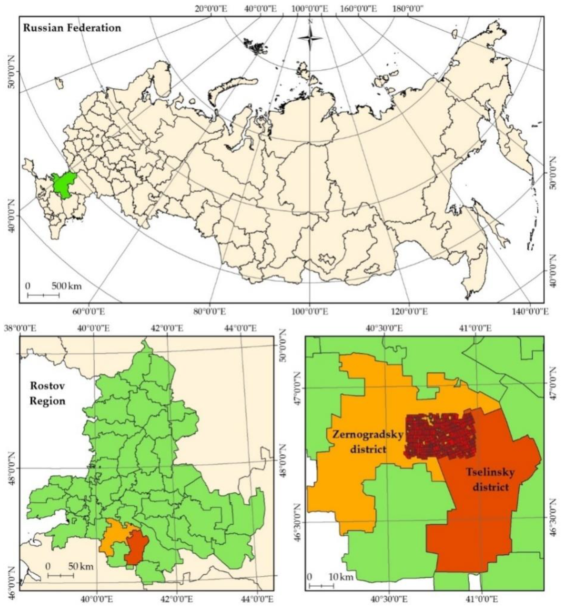
2. Materials and Methods

The studies were conducted on the territory of Russia in the Tselinsky and Zernogradsky districts of the Rostov Region (Figure 1). The soil cover is represented by low-humus thick ordinary calcareous chernozems, clayey and heavy loamy on loesslike clays (Haplic Chernozem (Loamic, Aric, Pachic)). Altitude is 100 m. The mean annual air temperature is 10.6 °C. The mean annual precipitation is 537.9 mm.

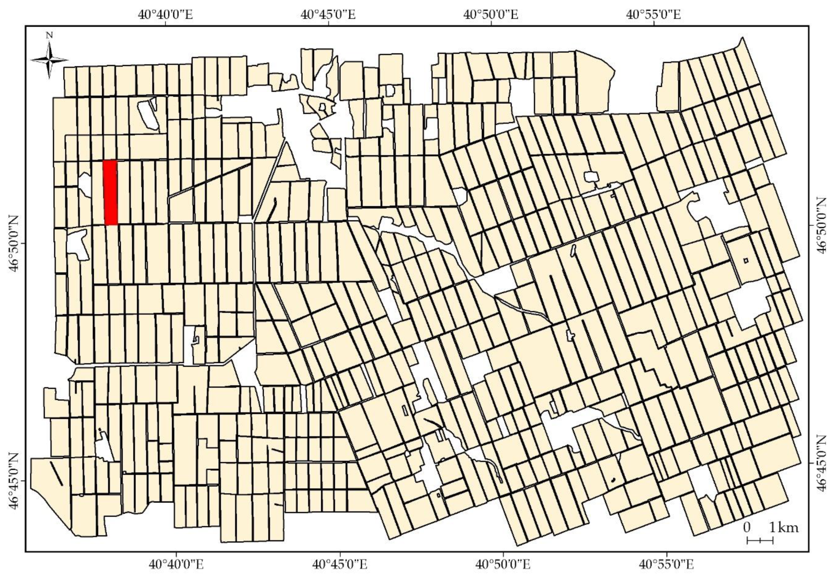
2.1. Setting Boundary Conditions for Interpretation

The spatial boundary conditions for degraded areas of arable land interpretation in this work are the boundaries of agricultural fields. To trace them, the method of retrospective monitoring of land use and soil cover is used [19]. This method is based on the manual interpretation of satellite imagery of different resolutions over the past 50 years. The method allows to allocate boundaries of agricultural fields with spatial accuracy of topographic maps on a scale of 1:10,000 [19,21] (Figure 2).
To find the boundaries of agricultural fields, a dataset for a period of 35 years (from 1984 to 2019) was formed. During this time, the cultivated area in Russia decreased from 117 million hectares (1990) to 74 million (2007) [59]. Then, cultivated area grew to 80 million hectares. (2019). For the formation of a dataset, the boundaries of agricultural fields for the entire period are needed [19]. Agricultural fields boundaries were created by manual interpretation of orthophotomaps (Figure 3) and satellite imagery of high spatial resolution (IKONOS, GeoEye-1, WorldView, etc.) [60], medium spatial resolution (Landsat, Sentinel) [31] and archival data from 1968 and 1975 (CORONA) [61]. Interpretation was verified using topographic maps of a scale of 1:25,000 (Figure 4). The accuracy of mapping the boundaries corresponded to a scale of 1:10,000. The boundary conditions were set for 536 agricultural fields; 530 agricultural fields (Figure 5) out of 536 were used for machine learning and creating a test sample; 6 out of 536 fields were used for acceptance sample and ground surveys (Figure 6).

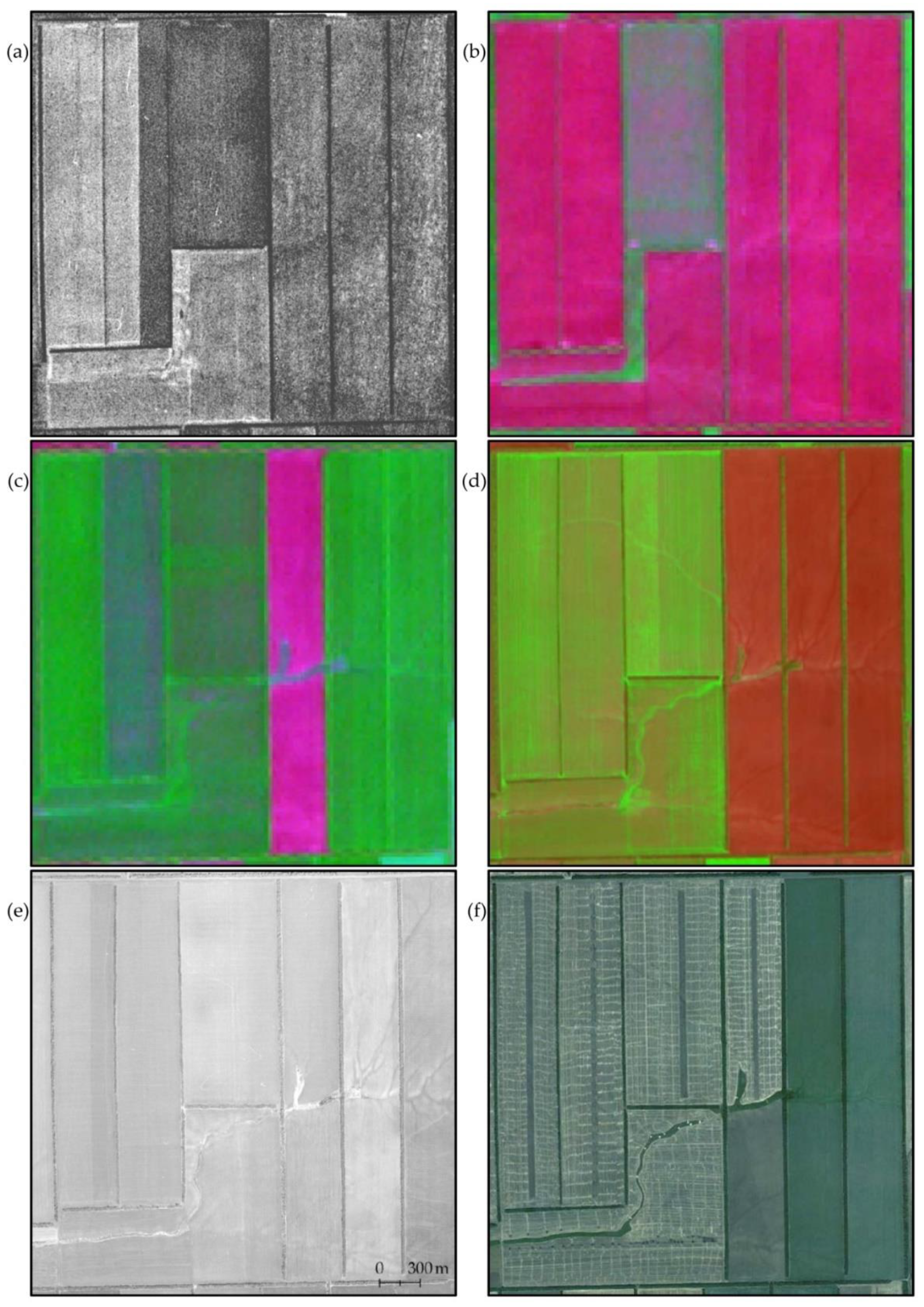
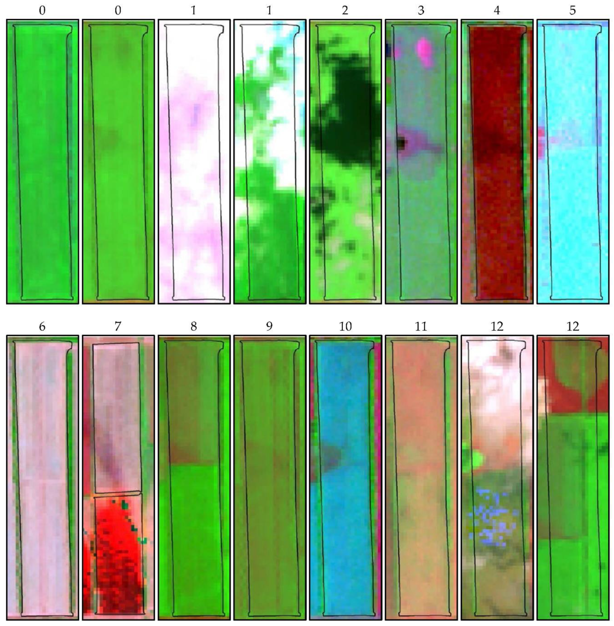
2.2. Formation of the Dataset

To form the dataset, Landsat 4, 5, 7 and 8 data were used. Landsat imagery ensures the longest maximum time series (35 years), the same spatial resolution (30 m), the uniform set of spectral bands (blue, green, red, NIR, SWIR1, SWIR2), and well-developed spectral calibration algorithms. The dataset was formed by visual analysis of 1028 Landsat data scenes for each agricultural field. The field boundaries obtained by setting the boundary conditions for degraded areas of arable land interpretation. For each pair “Landsat scene”/“agricultural field number”, the operator set in the table the value of the attribute of scene suitability for calculating vegetation indices for the entire field. For each agricultural field, the suitability of each Landsat scene was assessed. The analysis was carried out by three independent operators. In the case of differences in the values of the attributes set by them, the resulting value was chosen by a simple majority.
To create a dataset, 530 agricultural fields were selected on the territory of Tselinsky and Zernogradsky districts of the Rostov region of Russia (Figure 5). Fields are at the intersection of 173/028 and 174/027 Landsat path/rows. The training dataset was obtained for the Landsat path/row 173/028. In the archives, 531 scenes of Landsat 4, 5, 7, and 8 were found (Table S1). Dataset for the test sample was obtained for path/row 174/027, 497 Landsat 4, 5, 7, and 8 scenes were found in the archives (Table S2).
Another sixfields were used as the acceptance sample (Figure 6). For these fields, 497 scenes of the Landsat path/row 174/027 were used.
There are several factors that impede the calculation of vegetation indices within each agricultural field (Figure 7):
  • Cloud cover.
  • Cloud shadows.
  • Areas of waterlogging.
  • The open surface of the soil.
  • Snow.
  • Crop residues (straw).
  • Burning of crop residues.
  • Sowing of several crops or varieties of crops on one field.
  • Traces and errors of agrotechnical processing.
  • Ripening of crops.
  • Weed vegetation.
  • The defects or shift of remote sensing data.
For each of the 530 fields, the operators viewed all 1028 Landsat scenes. Scenes were viewed in the RGB mode. Landsat bands SWIR, NIR and green were stacked to view (Figure 7). Viewing was carried out by three operators independently. In case of contradictions in the selection results between operators, the correctness of selection was confirmed by a simple majority. Operators worked in binary selection mode. Initially, for each pair “Landsat scene”/“agricultural field number”, the value “0” was set. If the operator believed that the scene is suitable for further work on this agricultural field, he set the value to “1”. Examples of dataset for training and test samples are in Tables S1 and S2. The operator had to reveal all the reasons for the possible unsuitability of a particular Landsat scene for a specific agricultural field. Examples of Landsat data suitable for calculations are presented on Figure 7. Pairs “Landsat scene”/“agricultural field number” were considered suitable, when none of the 13 factors limiting the calculation of vegetation indices for the entire agricultural field was recorded. Dataset was created as part of a grant [62] and provided for this study by Agronote company [58].
The training sample consisted of 281,430 training elements. The test sample consisted of 263,410 training elements. The acceptance sample was 2982 training elements.

2.3. Machine Learning Methods

We exploit machine learning methods to determine whether satellite images are suitable for agricultural purposes.
Debatably the most popular machine learning algorithms of the past decade, Support Vector Machine (SVM) has been widely used in many fields, including agriculture. In several works, SVM was applied to classify satellite images, becoming a standard choice for visual recognition in agriculture [63,64,65,66]. At the same time, k Nearest Neighbors (KNN) algorithm was an alternative learning-based approach, used in various soil classification tasks [67,68,69,70].
However, SVM-like and KNN-like methods are severely outdated. In many fields, they have been displaced by more modern methods based on other working principles. Recently, deep learning-based approaches have been applied for soil classification. After exploring the best practices of solving an image classification problem, we decided to follow these practices to filter satellite images.
All machine learning methods can be subdivided into two large groups: classic methods and deep learning-based methods, both having pros and cons. To provide a full picture, we select one algorithm representing each of these groups. Specifically, we opt for two state-of-the-art techniques: classic Gradient Boosting on Decision Trees and deep learning-based Convolutional Neural Network. Below, we briefly describe these methods and explain how they can be applied to classify satellite images.

2.3.1. Gradient Boosting on Decision Trees

A Decision Tree is an acyclic connected graph where each internal node represents a check on a feature of a sample, each branch represents the result of this check, and each leaf node represents a class label (decision taken after checking the features). The paths from root to leaf represent classification rules.
More formally, Decision Tree for a domain X is a classification algorithm
f ( x ) = ( V i n , ν 0 , V o u t , S ν , β ν )
given by an acyclic connected graph, where
  • V = V i n V o u t is a set of vertexes, ν 0 V is a root of the tree,
  • S v :   { 0 , 1 } V ν is a predicate transition function to child nodes of a vertex ν ,
  • β ν :   X 0 , 1 is branching predicate for each ν V i n ,
  • Every ν V i n is associated with one class label y ν Y .
Multiple algorithms of building a Decision Tree have been proposed, such as ID3, C4.5 or CART. While being simple and intuitive, Decision Trees usually tend to overfit. To overcome this limitation, multiple decision trees are ensembled that results in a more robust model. The most powerful algorithm based on the Decision Trees is Gradient Boosting [71]. Its main idea is the consecutive construction of a sequence of Decision Trees by minimizing the differential loss function. While constructing the tree f t this loss function depends on the predictions of the already constructed tree ensemble f 1 , f t 1 on the entire dataset.
This paper solves the problem of binary classification, so the set of class labels Y = { 0 , 1 } . For each pair x X from the field and the satellite image the feature vector is built from statistical characteristics of pixel values of each channel intersecting the field interior.

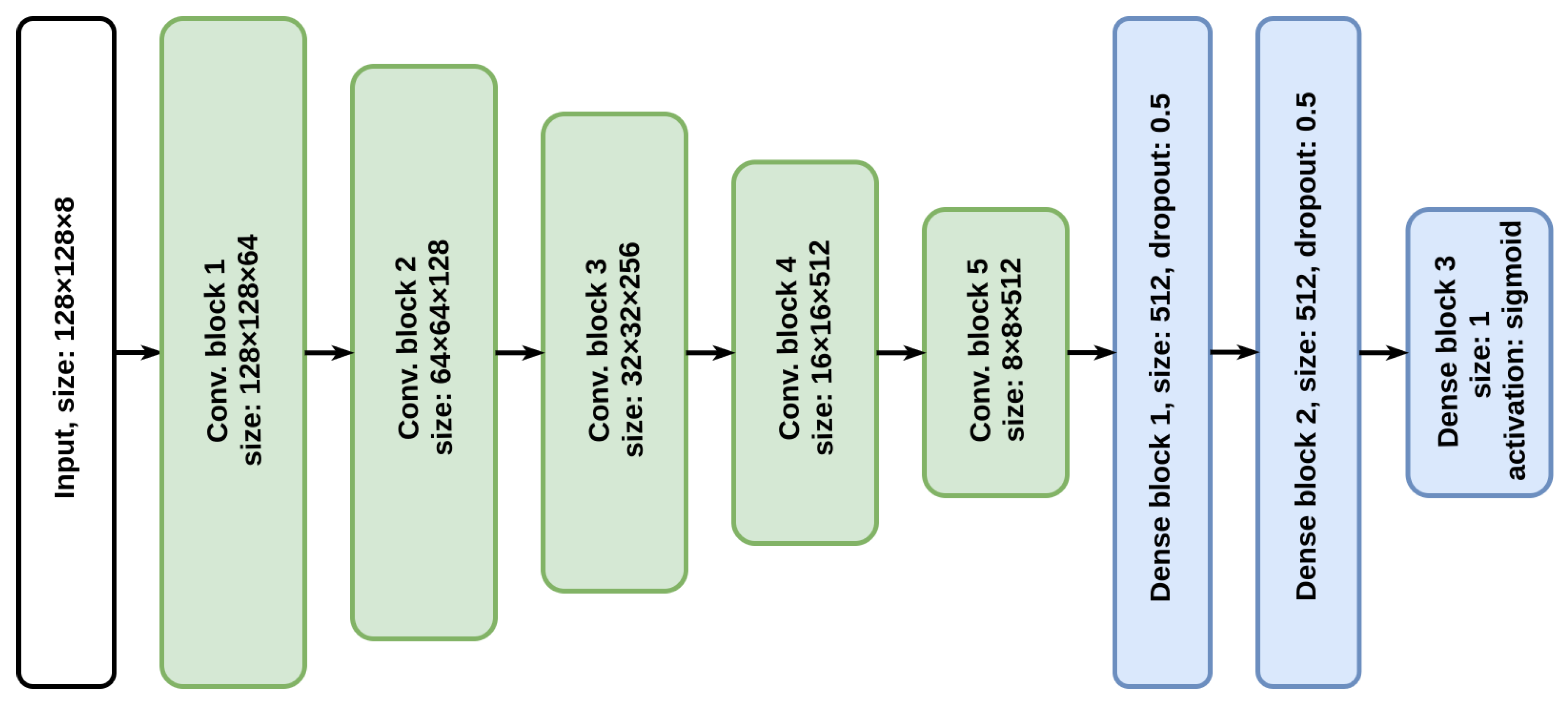
2.3.2. Convolutional Neural Network

Convolutional neural network (CNN) is specific neural network architecture, proposed by [72], originally aimed at an efficient image recognition. The main types of CNN layers are convolution, pooling, activation, normalization and fully connected. Convolutional layer is characterized by m × c square filters of size n × n and a bias. Such layer maps the input tensor x of shape w × h × c to the output tensor y of shape w × h × m following the equation:
y i , j k = i ` = 1 n j ` = 1 n l = 1 n W i , j k , l x i + i ` , j + j ` l + b k ,
for each 1 i w ,   1 j h , 1 k m . Here W and b are the weights of convolutional kernel as bias respectively.
Pooling layer reduces the spatial dimensionality of a tensor. Usually the image is divided into square blocks and from each block only one value is selected with an aggregation function, e.g., maximum or averaging. Activation layers aim to apply non-linearity to the output of the previous layer. Their typical representatives are sigmoid function:
σ ( x ) = 1 1 + e x ,
of rectified linear unit (ReLU):
R e L U ( x ) = max ( x , 0 ) .
Batch normalization layer was introduced in [73] to stabilize and speed up the process of neural network training. By normalizing the outputs of the previous layer to their expectation and variance, it allows the statistical characteristics to be kept constant.
Fully connected layer maps the input vector x of size n to an output vector y of size m following the equation:
y i = i = 1 n W i , j x i + b j ,
for each 1 j m . Here W and b are the weight and bias parameters with sizes n × m and m , respectively.
The neural network built from such layers is trained to minimize the value of the loss function by back-propagating the error value with stochastic gradient descent optimizer. In our case, the input of the neural network is a multi-band satellite image with a mask of a field. In turn, the output is a probability of belonging to one of two possible classes.

2.4. Methods for Assessing the Quality of Machine Learning Algorithms

  • Test sample. A set of objects not used in learning.
  • Acceptance sample. A set of objects not used in development.
  • Cross-validation [74,75]. The learning sample is divided into N parts and N—1 parts are trained N times (without repetitions).

2.5. Machine Learning Experiments

Machine learning was carried out using a dataset with 281,430 learning elements for the Landsat path/row 173/028 using the cross-validation method with N = 5. In our work, the task of binary classification of satellite images of fields into two classes depending on their suitability for analysis in agriculture is solved with the help of machine learning. For the training and test purpose the collected dataset is split in two almost equal parts. The training part contains Landsat scenes path/row 173/028 and the remaining scenes path/row 174/027 are used for testing. The final dataset contains 12,775 objects in positive and 532,065 objects in negative classes. In this imbalance, standard metrics, such as accuracy, precision or recall, are not representative when comparing models. We use the default in such cases area under curve (AUC) metric, which describes the area under the receiver operating characteristic (ROC) curve.

2.5.1. Gradient Boosting

As described above, one object from the training set is the pair “Landsat scene”/“agricultural field number”. The first step in the application of classical machine learning methods is the extraction of features from data. In experiments with gradient boosting, we describe one object with 71 features. One feature is the number of a day in a year when a satellite image is taken, while the remaining 70 are split into 10 features for each of the 6 bands: red, green, blue, NIR, SWIR1, SWIR2 and NDVI. To calculate the channel features, we present the values of all pixels of the corresponding channel intersecting the examined field as a one-dimensional distribution and consider its statistical characteristics. These 10 characteristics include standard deviation, skewness, kurtosis and percentiles with thresholds: 1%, 5%, 10%, 50%, 90%, 95%, 99%.
We use the CatBoost [76] library for the Python programming language to train the gradient boosting machine. Logistic function is used as a default loss for function for binary classification task. For two classes with labels y { 0 , 1 } and a predicted probability p the loss formula is
L o g L o s s ( y , p ) = y log p ( 1 y ) log ( 1 p ) .
The classifier is trained for 200 iterations with 0.01 learning rate. As the collected dataset is highly imbalanced, we set the weights of both classes not equal; more specifically, their values are 0.01 and 0.99. The achieved AUC metric on a test set for a trained gradient boosting classifier is shown in the firstline of Table 1.

2.5.2. Convolutional Neural Network

We suggest using the standard architecture of a convolution neural network for the binary classification task. Such architectures usually [72,77] consist of a couple of convolutional blocks follow by a pooling layer and another couple of fully connected layers. In turn, convolutional block contains a convolutional layer, a normalization layer, an activation layer and a maximum pooling layer. For each pair “Landsat scene”/“agricultural field number” we crop the corresponding region with size of 128 pixels. So, the shape of the input layer is 128 × 128 × 8; eight bands here include: red, green, blue, NIR, SWIR1, SWIR2, NDVI and a binary field mask.
As shown in Figure 8 the proposed neural network contains five convolutional blocks and three fully connected layers. Each convolutional layer is followed by Batch Normalization layer. The kernel size of each layer is equal to 3 and the padding value is 1. As an activation function after all convolutional and fully connected layers we use the ReLUfunction. All blocks end with an average pooling layer with factor 2. Two dropout layers with probability 0.5 are used between two pairs of dense layers to prevent overfitting. As we are predicting the probability for the second class classification problem, the last fully connected layer of size 1 is followed by sigmoid activation function.
As a loss function we use binary cross entropy, which in our case is equal to the equation above. This loss is minimized with a stochastic gradient descent optimizer Adam [78] for 10,000 steps with batch size of 64 and the learning rate 0.0001. Each batch contains 32 positive and 32 negative samples. The achieved AUC metric on a test set for a trained neural network is shown in the second line of Table 1.
The results in Table 1 show that both classical and deep learning methods reach accuracy above 98.5. In further experiments, the neural network will be used as it reaches a slightly higher value of the target metric. We also trained the best model on the test and training parts of the dataset together for adoption in further experiments to determine soil degradation on other fields and images. An example of the learning results is presented in Table S2. For each pair “Landsat scene”/“agricultural field number”, the probability of its suitability for calculations is given.

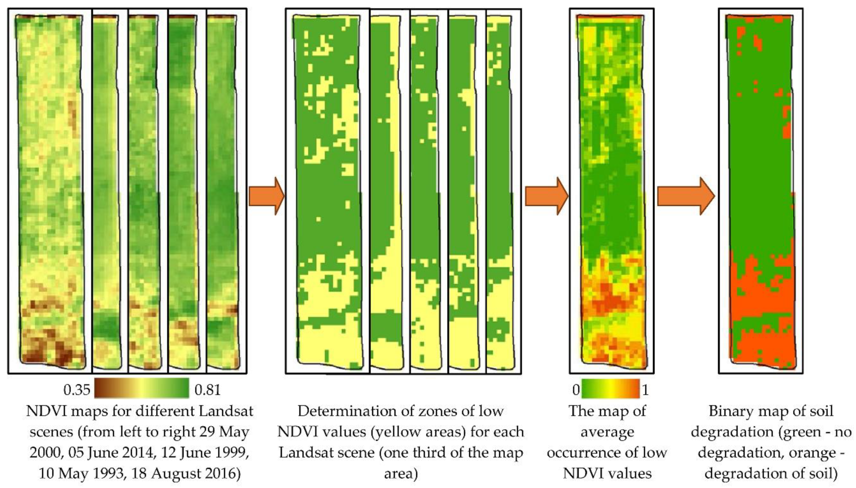
2.6. Calculation of Zones of Low NDVI Values (Zones of Reduced Fertility)

NDVI [79] is calculated for each pair of “Landsat scene”/”agricultural field number” marked in the dataset as suitable for calculations. Then, within the boundaries of agricultural fields, the areas of low NDVI values for the field are calculated. NDVI values of one-third of the field area and lower than the other two-thirds were considered low. Then the map is converted to binary form, where the low NDVI values make up one-third of the agricultural field. Field boundaries serve as boundary conditions.
The threshold value of one-third of the field area for low NDVI values was derived empirically from the experience of creating of task maps for precision farming based on the analysis of big data [30,52]. During the study, the fields were divided into 15, 9, 6, 3 and 2 zones of soil fertility equal in area. These were zones of the average long-term state of agricultural vegetation or the average long-term values of the vegetation indices [52]. To calculate task maps for precision farming, for most agricultural fields (80–90%), it turned out to be necessary and sufficient to divide them into three zones of fertility equal in area. The work was conducted on the territory of Rostov [52], Lipetsk [80], Tambov [14] and Krasnodar regions [30].

2.6.1. Calculation of the Zones of Low Values of NDVI (Zones of Reduced Fertility) Based on Data Selected by Machine Learning

For each pair “Landsat scene”/“agricultural field number” selected by machine learning, NDVI was calculated using the formula [79]:
NDVI = (RED − NIR)/(RED + NIR),
where
  • RED is the red band value after atmospheric correction [81,82,83].
  • NIR is the infrared band value channel after atmospheric correction.
  • Atmospheric correction was carried out using the ATCOR module of the ERDAS imagine software package [84].
An example of the results of calculation is shown in Figure 9.
For each NDVI calculation, the agricultural field was divided into tree equal areaswith NDVI values in the low, medium, and high ranges. Then, the zones of medium and high NDVI values were assigned the value “0”, and the zone of low NDVI values was assigned the value “1”. A series of binary maps of the distribution of low NDVI values for each agricultural field was obtained (Figure 9). Then, the summation of the values of binary maps for each pixel and division by the number of Landsat scenes selected for the agricultural field was carried out:
AOLNDVI = ( i = 1 n LNDVIi ) / n ,
where
  • AOLNDVI—average occurrence of low NDVI values;
  • LNDVIi—NDVI low zone indicator for the i-th Landsat scene;
  • n—number of Landsat scenes selected for calculations.
AOLNDVI value > 0.5 was taken as a zone of soil degradation. Divided by threshold value of 0.5, binary maps of soil degradation were created (Figure 10 and Figure 11).

2.6.2. Calculation of the Zones of Low NDVI Values (Zones of Reduced Fertility) Based on Manually Selected Data

A visual review of Landsat 174/027 data was carried out for six agricultural fields. The selection was similar to the selection during the creation of the dataset. Binary maps of degradation were calculated (Figure 12). The calculation was the same as the calculation of zones of low NDVI values (zones of reduced fertility) based on data selected using machine learning.

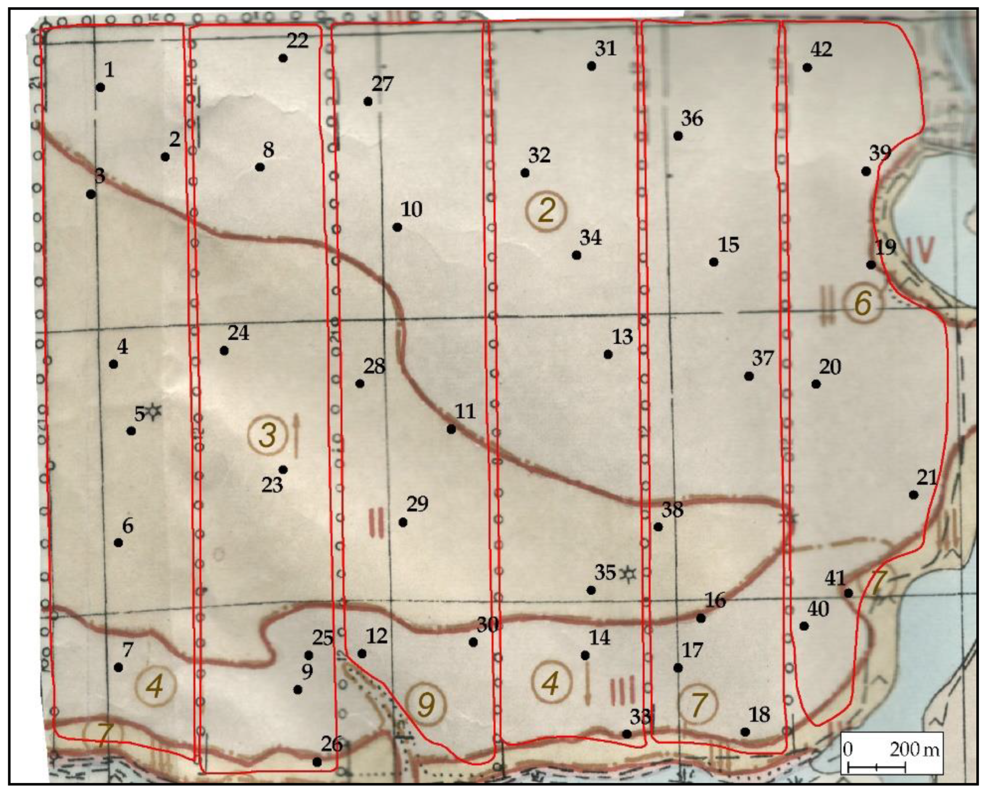
2.7. Ground Verification

Ground verification was carried out by classical methods of field soil research [1]. At the beginning, topographic maps and remote sensing data were analyzed. Then, field routes and detailed examination sites were planned. At each point of the ground survey, a soil pit was made. The soil profile is described and samples were taken. The coordinates of sampling and the location of the soil pits are fixed. Next, the analysis of the samples in the laboratory was performed.
Ground data for verification of maps of the soil degradation development were obtained in 2019. Overall, 42 soil pits on 6 agricultural fields on an area of 713.3 hectares were described and sampled. Two indicators were measured—the thickness of the humus horizon and the humus content in the plow horizon (Table 2). The thickness of the plow horizon was 25 cm. The humus content was determined by Tyurin’s (wet combustion) method with a photometric ending [85]. This method is analogous to the Walkley-Black method [86]. The location of the soil pits is shown in Figure 6, Figure 10, Figure 11 and Figure 12. Soil pits were located in places specified during the analysis of topographic maps and remote sensing data (Figure 6). Based on the analyses and descriptions of the soil profiles, the factor of soil degradation was determined. Degradation was judged from a decrease in the thickness of the humus horizon and/or humus content in the plow horizon. The presence/absence of degradation and its type are given in Table 2. In the description of soil profiles, 1is assigned to wind erosion, and 14 to water erosion.
Point 5 on the watershed and not having the catchment area was attributed to wind erosion. Points on slopes and in thalwegs were classified as water erosion. Point 6 can be attributed to both types of erosion. A similar division by the types of erosion is noted on the soil map of 1972 [87].
The interpretation accuracy was determined by the percentage of coincidences between the points of ground-based determination of the presence of soil degradation and maps of the distribution of soil degradation obtained by automated methods of multi-temporal remote sensing data interpretation (Table 2).

2.8. Cartographic Analysis
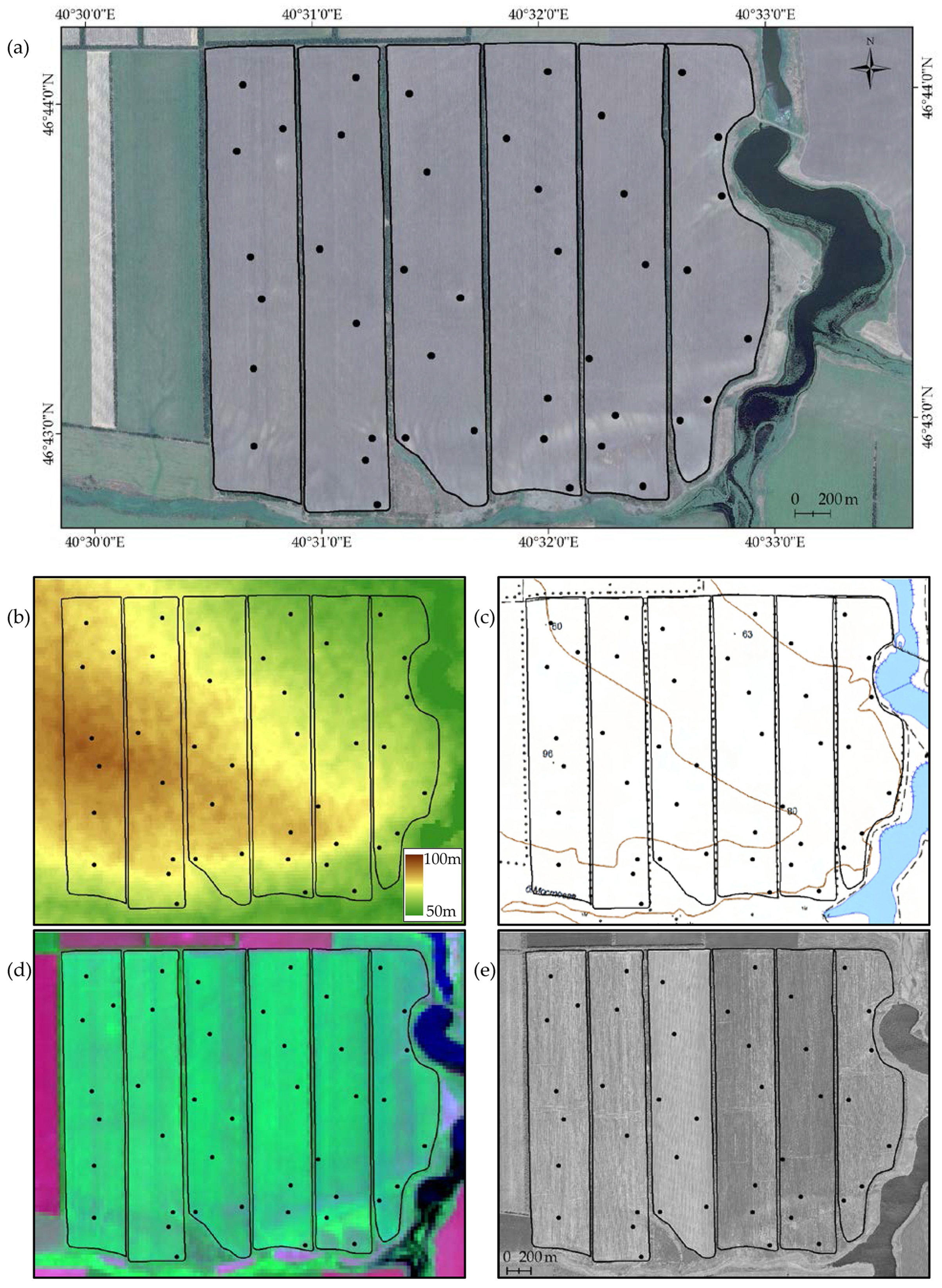
The materials obtained in this study were assembled into a GIS project in ArcGIS [88]. The analysis was carried out by pairwise intersection of GIS layers. Spreadsheets of possible combinations of intersected layers were created. Quantitative calculations and groupings of the resulting combinations were carried out.

2.9. GIS Project

To perform the analysis of the research area, a GIS project of the following composition was created:
  • Topographic map on a scale of 1:25,000.
  • Aerial photography of 2012. Panchromatic orthophotomap with a spatial resolution of 0.6 m.
  • Digital elevation model (SRTM), horizontal resolution is 1 arc second and vertical 1 m.
  • Space survey of 1968 with a spatial resolution of 1.8 m. Panchromatic survey, satellite KH-4B, mission CORONA USA.
  • Space survey of 1975 with a spatial resolution of 6 m. Panchromatic survey, satellite KH-9, mission CORONA USA.
  • Remote sensing data Landsat 4, 5, 7 and 8 from 1984 to 2019 (1028 scenes).
  • Remote sensing data Sentinel-2 2019 (7 tiles).
The exact geographic referencing of the remote sensing materials 2, 4, 5 was carried out by locally affine transformations using a topographic map at a scale of 1:10,000. Atmospheric correction and spectral transformations were not carried out. For data 6 and 7, atmospheric correction was made using the ATCOR module of the ERDAS imagine software package [63].
The GIS project was used for visual analysis and determination of field boundaries by the method of retrospective monitoring of the soil and land cover. Only Landsat data were used to calculate soil degradation maps using machine learning.

3. Results

3.1. Predicting the Suitability of Satellite Imagery Frames for Acceptance Sample

Based on machine learning, a prediction was made of the suitability of satellite imagery for calculating vegetation indices. The prediction was made for six agricultural fields (Figure 6). Landsat scenes 174/027 were analyzed. In total, 497 Landsat 4, 5, 7, 8 scenes were found in archives for this path/row. The probability of suitability for calculations was calculated 2982 times. The results are presented in Tables S3 and S4.
The selection of fields for acceptance sample was determined by the possibility to obtain ground data. The territory for data collection was determined by the owner of agricultural land. The owner showed interest in identifying degraded territories on his lands, but in a limited area.

3.2. Addition to the GIS Project

Based on the results of the study, the following layers were added to GIS project:
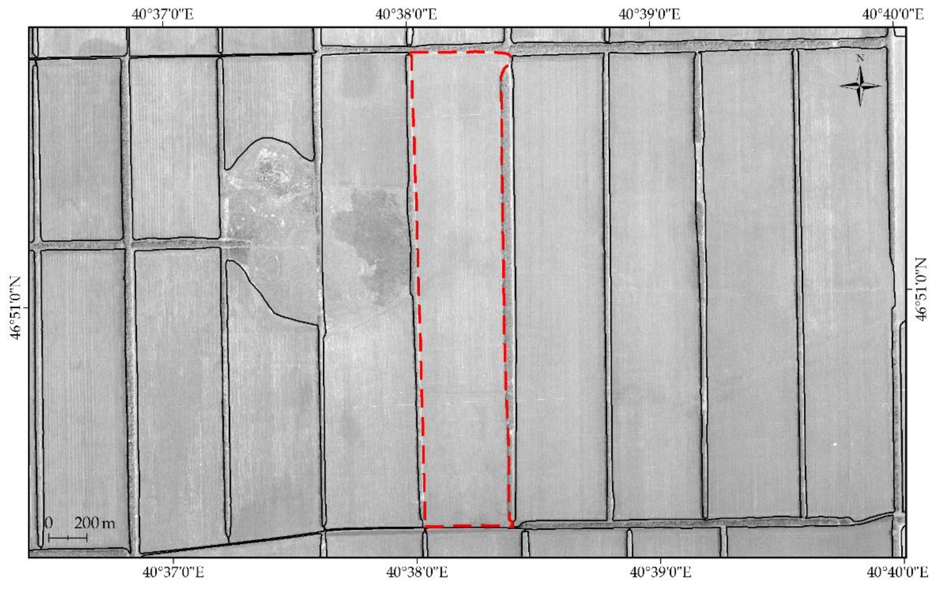
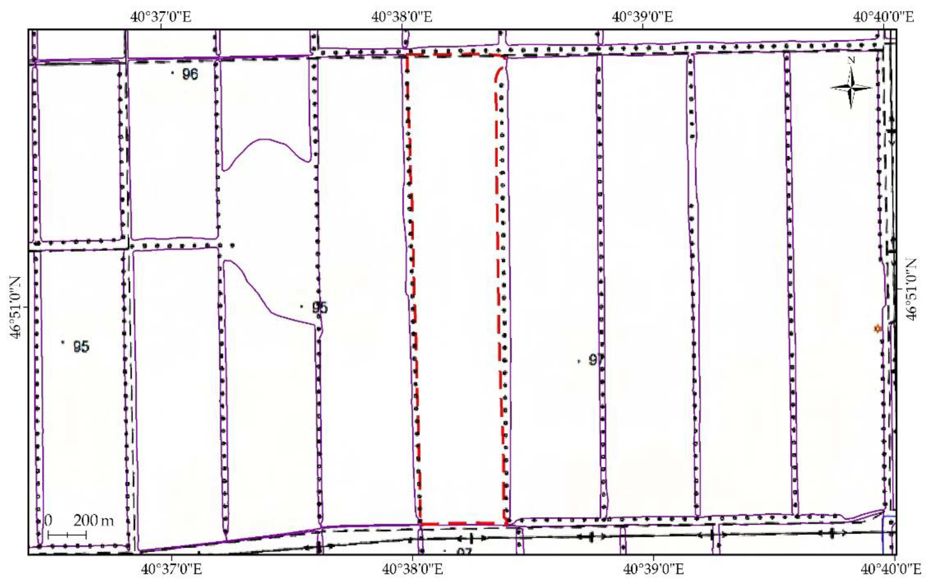
  • The scheme of agricultural fields (the boundaries of interpretation and recognition).
  • Binary map of the degradation development calculated using Landsat data selected by a neural network (Figure 10).
  • Binary map of the degradation development calculated using Landsat data selected by gradient boosting (Figure 11).
  • Binary map of the degradation development calculated using Landsat data selected by visual viewing (Figure 12).
  • Map of the location of the results of ground surveys (map of soil pits).

3.3. Comparison of Degradation Development Maps Obtained Using Different Methods of Satellite Imagery Selection

In total, the presence/absence of degradation was calculated for 7926 pixels, for 6agricultural fields on an area of 713.3 hectares. The area of degradation was:
  • for manual selection of Landsat scenes—156.5 hectares;
  • for Landsat scenes selection using gradient boosting—145.7 hectares;
  • for Landsat scenes selection using neural network—149.5 hectares.
The area of discrepancies between binary maps of degradation distribution for manual selection of Landsat scenes and selection by gradient boosting was 38 hectares. (5.3%). The area of discrepancies between the binary maps of degradation distribution for manual selection of data and neural network selection was 40 hectares. (5.6%). The areas of discrepancies between the two maps constructed using machine learning methods was 21.4 ha. (3%) (Table 3).
Maps of areas of degradation distribution obtained by different methods of selecting Landsat scenes have high convergence (more than 94%). Consequently, deep machine learning methods can be used to replace manual sampling of remote sensing data. In this case, the discrepancy will amount to about 5% with some underestimation of the areas of distribution of degradation.

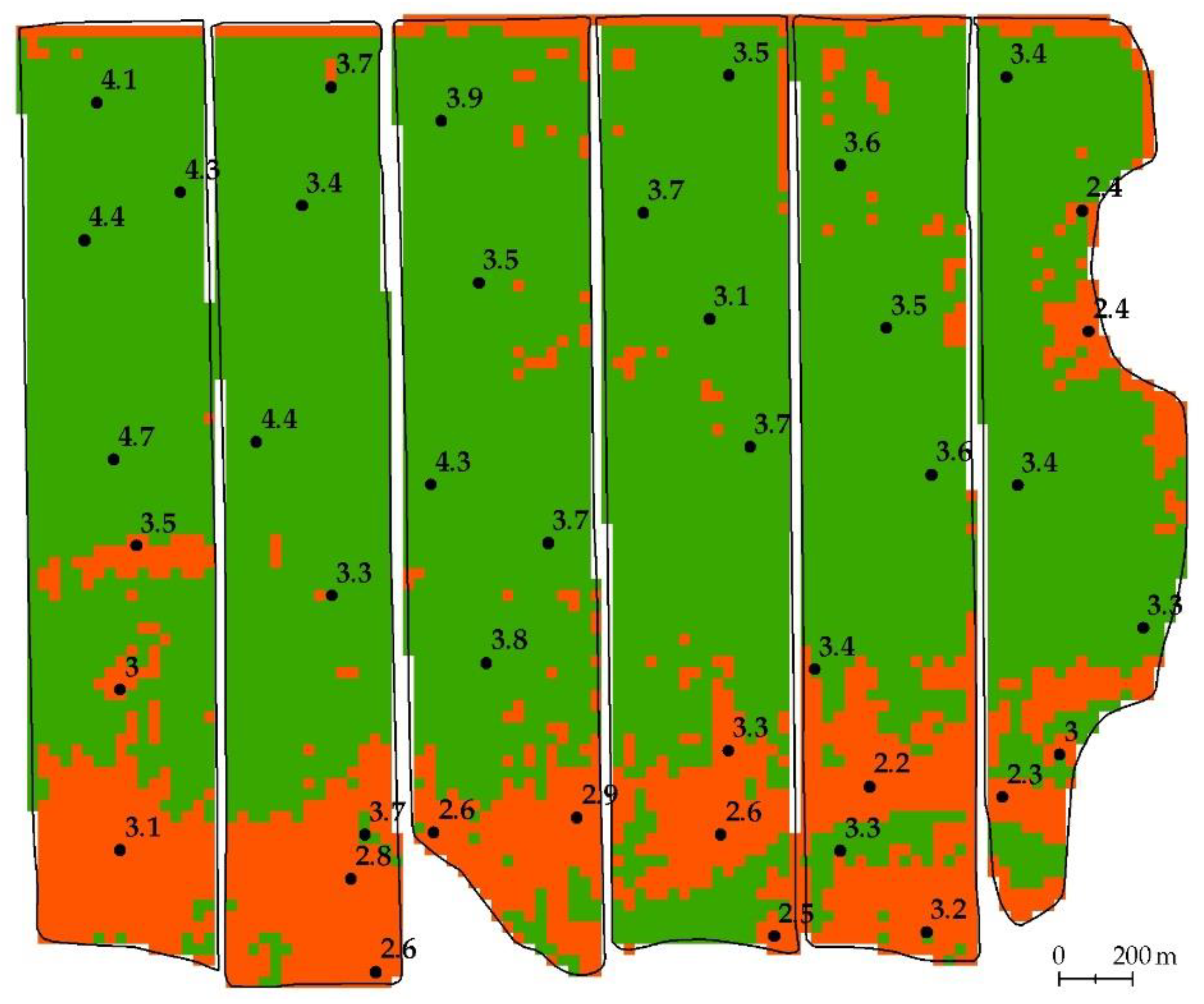
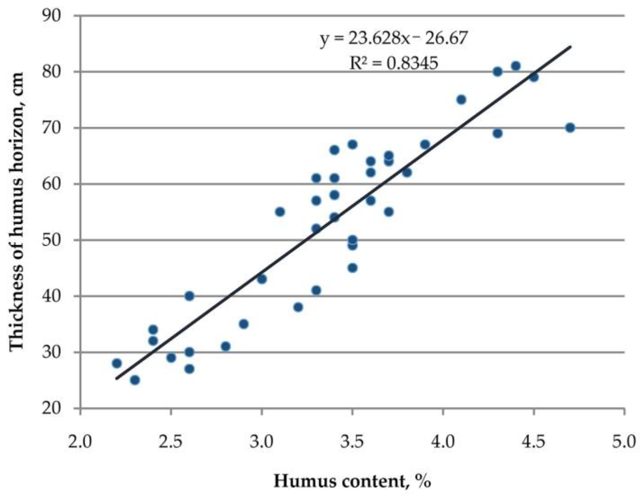
3.4. Ground Verification of Degradation Maps

Figure 10 shows a map of soil degradation development. The map is based on the selection of satellite imagery using deep machine learning methods. The map shows the areas of the most probable occurrence of low vegetation indices for 35 years. Thus, the map is the result of the analysis of big satellite data [28,29]. To create a map, an analysis of 497 Landsat scenes was performed. Machine learning in this paper is a tool for data mining [36,37].
Figure 6, Figure 10, Figure 11 and Figure 12 show the location of soil pits. In Figure 10, soil pits are on binary maps of degradation. Note that the maps of degradation distribution were created completely automatically without ground calibration. According to Table 2, it is possible to calculate the average values of the humus content for the degradation zone and for the zone where degradation does not occur. The average value of the humus content is 2.8% for degraded soils and 3.7% for non-degraded soils. Both zones are statistically significantly different according to analysis of variance (ANOVA) (Table 4). The thickness of the humus horizon is 39.5 cm for degraded soils and 63.9 cm for non-degraded soils. Both zones are also statistically significantly different (Table 5).
The results obtained are in good agreement with the general characteristics of the main soil of the region. Such soil is a low-humus thick ordinary calcareous chernozem [89]. It is characterized by the humus horizon of 60–80 cm in thickness and the humus content of 3–6%. A decrease in the humus content to less than 3% and/or a decrease in the thickness of the humus horizon to less than 50 cm can be considered indications of degradation development. In such cases, the soil is classified as eroded chernozem [87,90] (Table 2).
The analysis of Table 2 shows that all of three binary degradation maps divided field data into completely identical groups. Calculation of accuracy based on ground data for any of the three maps was also identical. In this regard, a single calculation of the accuracy of maps is given.
Both attributes of degradation are highly correlated (Figure 13). Indeed, the humus content decreases with the depth in the soil profile. During degradation (erosion) process, partial or complete loss of the upper soil horizons occurs. With the loss of the upper soil layers, both the thickness of the humus horizon and the humus content in the upper horizon decrease.
Obtained by the analysis of big satellite data, maps of the distribution of degradation should be evaluated for accuracy within the framework of the information theory. The values of the first and second type of errors should be established. According to the information theory, we have errors of the first (α errors, false positive) and second type (β errors, false negative). In this study, type I errors mean that the method predicts degradation, where it does not exist. Type II errors mean that the method does not predict degradation, where it really exists. The value of type I error was 12.5%. The value of type II error was 3.8% (Table 2).
Consequently, maps of the development of degradation obtained by analyzing big satellite data make it possible to identify areas of distribution of degraded soils.
Thus, a system for predicting the development of soil degradation on arable land has been created. This system allows to automatically predict the areas of the most likely occurrence of soil degradation within agricultural fields under given boundary conditions. The probability of prediction in this study was 87.5%.

4. Discussion

4.1. Sources and Methods of Soil Erosion Detection

The main source of information on the distribution of soil degradation in Russia is soil maps. There is a scale series of soil maps with information on water and wind erosion: 1:10,000–25,000 (Figure 14) [87], 1:50,000–100,000 [90], 1:200,000–350,000, 1:2,500,000. Maps of scales 1:10,000–100,000 were made according to the all-Union instruction on soil surveys and the compilation of large-scale soil land use maps [1]. For a field survey, the instruction requires the use of topographic maps (Figure 6c) and orthophotomaps (Figure 6e). In fact, the boundaries of the areas with eroded soils on the large-scale soil maps were drawn using the relief characteristics as displayed on topographic maps of scales 1:10,000–25,000. The main factors taken into account were slope steepness and length for water erosion and elevated watershed landforms for wind erosion. Thus, such maps represented a model or erosion or potential erosion of the territory rather than actual erosion. The problem of determining the actual distribution of erosion on these maps was not solved. The use of remote sensing data in the form of orthophotomaps was mainly for reference purposes.
The actual distribution of soil degradation can be determined based on manual interpretation of large arrays of remote sensing data for the period from 1968 to 2020. Such work was and is being performed on the territory of the Rostov region of Russia [14,15,16,17,18]. In contrast to soil maps, where areas of potential degradation are determined according to relief factors, the interpretation of multi-temporal remote sensing data allows detecting areas of actual distribution of soil degradation. When analyzing multi-temporal remote sensing data, information about the relief is for reference purposes. Manual interpretation of multi-temporal remote sensing data allows obtaining accurate and good maps, but it is very laborious.
Modern methods of erosion detection often use erosion models [2,3,4,5]. These methods are a further development of the methods for analyzing relief parameters (slopes, exposure, catchment area, etc.) [8,9,10,11]. That is, like the soil maps, they show the areas of potential distribution of degradation (erosion).
It should be noted that mapping of erosion differs sharply from mapping of soil salinity [91] or electrical conductivity of soils [92]. When mapping soil salinity, the main source of information is remote sensing data and the actual distribution of the degradation factor is mapped [16,93].
The development of machine learning methods for detecting degradation is based on the same set of morphometric indicators and climatic data and requires more and more accurate digital elevation models [94,95,96]. Obtaining detailed DEMs (higher resolution than SRTM) is currently still a rather laborious and costly procedure.
Approaches to detecting degradation based on vegetation indices [21,22,23] do not require large expenditures of manual labor, do not require the construction of complex DEMs, and make it possible to determine the actual distribution of degradation factors [24,25,26]. The accuracy of work increases when using multi-temporal series [26].
In our study, we propose a method of degradation detection based only on available remote sensing data from open sources of information. The method detects the actual distribution of degradation. Degradation indicator is the depression of crops during a long time interval (35 years, 1984–2019). Automation of the selection of remote sensing data is achieved by using deep machine learning. The accuracy of the method is 87.5% at a spatial resolution of 30 m.
In general, the method has shown high efficiency with low requirements for information sources, which makes this method promising for mapping erosion on arable land.

4.2. Analysis of the Causes of Errors

The soils of the ground research points 7 and 41 have a thickness of the humus horizon of 76 and 78 cm and the humus content of 3.0% and 3.1% (Table 2). These values do not allow classifying these soils as degraded soils. However, such a combination of the great thickness of the humus horizon and relatively low humus content is not characteristic of the studied soils. Normally, their humus horizons are 60 to 80 cm in thickness, and their humus content is 3–6%. As the graph in Figure 13 shows, with increasing thickness of the humus horizon, the humus content should also increase. At these points for a thickness of 76 and 78 cm, the humus content of 4% or more is expected. Upon field identification, these soils were assigned to aggraded soils in local depressions on the slope. Such aggraded (water-deposited) soils are also a consequence of degradation processes, but they differ from “normal” degraded soils in terms of the thickness of the humus horizon. They were excluded from the calculation of the regression equation shown in Figure 13.
It was not possible to establish the reasons for a decrease in the thickness of the humus horizon less than 50 cm for point 15 (Table 2).

4.3. Analysis of Previously Created Maps of Soil Cover Degradation

Figure 14 shows the soil erosion map of the study area [87] created according to the all-Union instruction [1] in 1983. There are also earlier soil-erosion maps for this territory [90]. On the map (Figure 14), areas of arable land with distribution of water and wind erosion are indicated. The area of eroded soils according to the soil map is 351.2 ha. The total mapped area is 713.3 ha. (Figure 10, Figure 11, Figure 12 and Figure 14). Out of 42 points of ground verification, 24 points fall on polygons with eroded soils, and 18 points fall on soil polygons without erosion.
Out of 24 points within the polygons with soil erosion, erosion was really detected in 12 points according to ground data; in the other 12 points, it was not detected. Thus, the probability of finding non-eroded soils is 50%.
Out of 18 points within the polygons with non-eroded soils, erosion was absent in 15 points; however, in 3 points, it was detected during the field survey. Thus, the probability of finding eroded soils within such polygons is 16%.
It is obvious that the area of eroded lands on the map of soil erosion is overestimated by about two times. The area of real erosion distribution should be about 175 hectares. This value correlates well with the results of the methods described in our study (150 ha of eroded land).
Indeed, erosion modeling methods tend to overestimate the areas of actual soil erosion, because they provide an estimate of the area of potential rather than actual erosion.

4.4. Physical Interpretation of Work Technology

There is a discussion about the need for a physical interpretation of statistical dependences obtained using artificial intelligence [97]. Physical interpretation is understood as the presence of regression models linking one or another calculated characteristic of remote sensing data and soil property measured during ground work [98,99]. Indeed, in this way it is possible to establish the parameters of the regression between the NDVI and the properties of the arable horizon (the content of humus, phosphorus, potassium, zinc, etc.). The disadvantages of such models are their low applicability outside the modeling region and their high sensitivity to the type of remote sensing data.
There are much more sophisticated approximation methods for building functional models. For mapping the soil cover, the methods of piecewise linear and elastic approximation were used [100,101]. It significantly improved the results of applying linear regressions. Such methods make it possible to transform the N-dimensional space of spectral characteristics into a soil map.
In this study, methods that exclude the use of regression models were proposed. Our work consistently applies the principles of binary logic and measuring the frequency of occurrence of a binary attribute (low NDVI value) in big satellite data [102]. The distribution of this attribute on single Landsat scene is not an independent characteristic with this approach typical for big data analysis.
Indeed, low NDVI values in each specific year may be due to soil degradation factors, weather fluctuations, flaws in agricultural technology, properties of a particular crop, etc. Thus, one-third of the field with low NDVI values for a particular year cannot be interpreted as the development of soil degradation. A completely different situation arises when analyzing a set of binary maps of low NDVI values over 35 years for the same territory. If on dozens of Landsat scenes over 35 years the pixel value mostly (more than 50%) fell into the zone of low NDVI value, then it can be assumed that soil fertility is reduced in this part of the field. In areas with low soil fertility, it is possible to assume the presence of degraded soil cover. This assumption was confirmed in the course of field work. The areas of degradation were characterized by a low humus content in the arable horizon (25 cm) and alow thickness of the humus horizon.

4.5. Promising Remote Sensing Data

In this work, approaches to the analysis of big remote sensing data were implemented. Our hypothesis was that it was sufficient to select fragments of space imagery suitable for NDVI calculations for a specific field from the large remote sensing data. Thus, it was possible to use all suitable scenes without special filters for phenophases, crops, climate, etc. As follows from the work, a binary dataset is sufficient. For training, only two values for each pair “Landsat scene”/“agricultural field number” were used: “0” and “1”. For the purity of testing the hypothesis about the possibility of using a convolutional neural network for the selection of satellite imagery using a binary dataset, Landsat 4, 5, 7 and 8 data were chosen because of the longest continuous data series (35 years); the same spatial resolution (30 m); the uniform set of spectral bands (blue, green, red, NIR, SWIR1, SWIR2); common methods of geometric, atmospheric and radiometric correction; and open access. The correctness of the choice was confirmed by the volume of information of the same type—1028 Landsat scenes per study area. The training results were obtained using six bands of Landsat with a resolution of 30 m.
The Terra ASTER and Sentinel 2A,B sensors have similar spectral characteristics and spatial resolution to Landsat data. The ASTER archive is extremely poor and unsuitable for training a neural network with an extremely unbalanced training. The Sentinel 2A,B archive has a very small temporal coverage at the moment, which limits its teaching capabilities.
The limitations of the open archives of ASTER and Sentinel for training neural networks does not mean that the data from ASTER and Sentinel cannot be used to create maps of the distribution of soil degradation. The most promising direction is the inclusion of Sentinel in the calculations. To select Sentinel tiles, you can use a neural network trained on the Landsat data. For this, you need to apply several specific techniques. These techniques seem to be promising, they are currently under development. Integration of Sentinel into calculations is facilitated by a well-developed spectral and spatial correction of Sentinel data in relation to Landsat data.
The situation with the ASTER data is somewhat more complicated. These data need to be calibrated against to Landsat data. Otherwise, the techniques for including ASTER data into the system based on a neural network and calculating soil degradation maps should be similar to Sentinel. Upon completion of the integration of the Sentinel 2A,B data, work on the integration of ASTER data into the calculations will begin.
The possibilities of using a neural network trained on Landsat 4, 5, 7, 8 data for the selection of satellite imagery of other sensors (except for ASTER and Sentinel 2A,B) have not been studied by the authors at the moment.
Expansion of remote sensing data sources for creating soil degradation maps is a promising direction for further research.

5. Conclusions

In determining the objectives of the study, five assumptions were made. In the course of the work, all assumptions were confirmed. Indeed, areas of soil degradation development were identified based on the analysis of the vegetation index (NDVI). Areas with low long-term average NDVI values are indicators of parts of agricultural fields, in which soil degradation takes place. Long-term average occurrence of low NDVI values was obtained by analyzing big satellite data for 35 years (497 Landsat scenes). The selection of satellite data for calculations was based on deep machine learning. The boundary conditions of the calculations were determined by the methods of retrospective monitoring of land use and soil cover. The verification of automated calculations was carried out by classical soil field surveys.
Our study demonstrated that deep machine learning for remote sensing data selection is possible based on a binary dataset. This allows not to use intermediate filtering systems for the adequate selection of satellite imagery. It is possible not to determine clouds, shadows from clouds, open soil surface, etc. Direct selection of Landsat scenes suitable for calculations was made using deep machine learning tools, which greatly contributed to automation of mapping degraded soils.
The study did not reveal significant advantages of convolutional neural networks over gradient boosting in the selection of satellite imagery. Based on current research, both methods can be recommended. However, the main goal of the work was to test the possibilities of using deep machine learning. Gradient boosting was studied to compare the capabilities of different machine learning methods with manual data selection technology.
As a result of the work, a method for indicating degraded arable land areas was created. The method is based on deep machine learning and the calculation of average occurrence of low NDVI values. Low NDVI values were calculated separately for each suitable fragment of the satellite image within the boundaries of each agricultural field. NDVI values of one-third of the field area and lower than the other two-thirds were considered low. In the calculations, about 500 Landsat scenes were processed from 1984 to 2019 for each agricultural field. The method includes the following steps:
  • Setting the boundary conditions of the calculation.
  • Neural network filtering of satellite images in predetermined boundary conditions.
  • Calculation of low NDVI values from satellite images selected by the neural network.
  • Calculation of average occurrence of low NDVI values over 35 years.
  • Classification of average occurrence of low NDVI values to highlight areas of potential degradation.
For the method of indicating degraded arable land areas, type I and II errors were calculated for six agricultural fields of acceptance sample. Type I error was observed in 12.5% of cases, and type II error in 3.8%. Errors were calculated based on 42 ground survey points on the total area of 713.3 ha. Out of 42 points, 26 points were in areas where no degradation was automatically predicted, and 16 points were in areas where degradation was automatically predicted. During the field survey, indications of soil degradation were found in 15 points: 14 points in the area of predicted degradation and 1 point beyond. Thus, degradation was correctly predicted in 14 ground-verified cases.
The proposed method for indicating degraded arable land can be used in automated mapping of degraded soils. In arable land degradation areas identified by the proposed method, the probability of detecting soil degradation by ground-based methods is 87.5%. The probability of detecting soil degradation by ground-based methods beyond the predicted areas is 3.8%.

Supplementary Materials

The following materials are available online at https://0-www-mdpi-com.brum.beds.ac.uk/2072-4292/13/1/155/s1, Table S1: The example of training dataset for one agricultural field (Figure 3, Figure 4 and Figure 5), Table S2: The example of learning results for one agricultural field (Figure 3, Figure 4 and Figure 5): the probability ofLandsat scenes suitability for calculations is given. The probability is measured from 0 to 1, Table S3: Machine learning results for the acceptance sample (Figure 6) part 1: the probability of Landsat scenes suitability for calculations is given. The probability is measured from 0 to 1; gb—gradient boosting; nn—neural network; ms—manual selection, Table S4: Machine learning results for the acceptance sample (Figure 6) part 2: the probability of Landsat scenes suitability for calculations is given. The probability is measured from 0 to 1; gb—gradient boosting; nn—neural network; ms—manual selection.

Author Contributions

Conceptualization, D.I.R.; methodology, P.V.K. and D.I.R.; software, D.D.R.; validation, N.V.K. and P.V.K.; formal analysis, D.D.R. and P.V.K.; investigation, N.V.K. and D.I.R.; data curation, N.V.K.; writing—original draft preparation, D.I.R.; writing—review and editing, P.V.K.; visualization, P.V.K.; project administration, D.I.R. All authors have read and agreed to the published version of the manuscript.

Funding

This research received no external funding.

Institutional Review Board Statement

Not applicable.

Informed Consent Statement

Not applicable.

Data Availability Statement

Publicly available Landsat datasets were analyzed in this study. This data can be found here: http://earthexplorer.usgs.gov.

Conflicts of Interest

The authors declare no conflict of interest.

References

  1. All-Union Instruction on Soil Surveys and the Compilation of Large-Scale Soil Land Use Maps; Ischenko, T.A. (Ed.) Kolos: Moscow, Russia, 1973. (In Russian) [Google Scholar]
  2. Farifteh, J.; Van Der Meer, F.; Atzberger, C.; Carranza, E.J.M. Quantitative analysis of salt-affected soil reflectance spectra: A comparison of two adaptive methods (PLSR and ANN). Remote Sens. Environ. 2007, 110, 59–78. [Google Scholar] [CrossRef]
  3. Higginbottom, T.P.; Symeonakis, E. Assessing Land Degradation and Desertification Using Vegetation Index Data: Current Frameworks and Future Directions. Remote Sens. 2014, 6, 9552–9575. [Google Scholar] [CrossRef] [Green Version]
  4. Ibrahim, Y.Z.; Balzter, H.; Kaduk, J.; Tucker, C.J. Land degradation assessment using residual trend analysis of GIMMS NDVI3g, soil moisture and rainfall in sub-Saharan west Africa from 1982 to 2012. Remote Sens. 2015, 7, 5471–5494. [Google Scholar] [CrossRef] [Green Version]
  5. Mendonça-Santos, M.D.L.; Dart, R.O.; Santos, H.G.; Coelho, M.R.; Berbara, R.L.L.; Lumbreras, J.F. Digital Soil Mapping of Topsoil Organic Carbon Content of Rio de Janeiro State, Brazil. In Digital Soil Mapping; Boettinger, J.L., Howell, D.W., Moore, A.C., Hartemink, A.E., Kienast-Brown, S., Eds.; Springer: New York, NY, USA, 2010; pp. 255–266. [Google Scholar]
  6. Romanenkov, V.; Smith, J.; Smith, P.; Sirotenko, O.D.; Rukhovitch, D.I.; Romanenko, I.A. Soil organic carbon dynamics of croplands in European Russia: Estimates from the “model of humus balance”. Reg. Environ. Chang. 2007, 7, 93–104. [Google Scholar] [CrossRef]
  7. Rukhovich, D.I.; Koroleva, P.V.; Vilchevskaya, E.V.; Romanenkov, V.; Kolesnikova, L.G. Constructing a spatially-resolved database for modelling soil organic carbon stocks of croplands in European Russia. Reg. Environ. Chang. 2007, 7, 51–61. [Google Scholar] [CrossRef]
  8. Glazunov, G.P.; Gendugov, V.M. A full-scale model of wind erosion and its verification. Eurasian Soil Sci. 2003, 36, 216–226. [Google Scholar]
  9. Larionov, G.A.; Dobrovol’skaya, N.G.; Krasnov, S.F.; Liu, B.Y. The new equation for the relief factor in statistical models of water erosion. Eurasian Soil Sci. 2003, 36, 1105–1113. [Google Scholar]
  10. Maltsev, K.A.; Yermolaev, O.P. Potential Soil Loss from Erosion on Arable Lands in the European Part of Russia. Eurasian Soil Sci. 2019, 52, 1588–1597. [Google Scholar] [CrossRef]
  11. Sukhanovskii, Y.P. Rainfall erosion model. Eurasian Soil Sci. 2010, 43, 1036–1046. [Google Scholar] [CrossRef]
  12. A Shary, P.; Sharaya, L.S.; Mitusov, A.V. Fundamental quantitative methods of land surface analysis. Geoderma 2002, 107, 1–32. [Google Scholar] [CrossRef]
  13. SRTM. Available online: http://srtm.csi.cgiar.org (accessed on 20 July 2020).
  14. Koroleva, P.V.; Rukhovich, D.I.; Shapovalov, D.A.; Suleiman, G.A.; Dolinina, E.A. Retrospective Monitoring of Soil Waterlogging on Arable Land of Tambov Oblast in 2018–1968. Eurasian Soil Sci. 2019, 52, 834–852. [Google Scholar] [CrossRef]
  15. Rukhovich, D.I.; Simakova, M.S.; Kulyanitsa, A.L.; Bryzzhev, A.V.; Koroleva, P.V.; Kalinina, N.V.; Chernousenko, G.I.; Vil’Chevskaya, E.V.; Dolinina, E.A. The influence of soil salinization on land use changes in azov district of Rostov oblast. Eurasian Soil Sci. 2017, 50, 276–295. [Google Scholar] [CrossRef]
  16. Rukhovich, D.I.; Simakova, M.S.; Kulyanitsa, A.L.; Bryzzhev, A.V.; Koroleva, P.V.; Kalinina, N.V.; Chernousenko, G.I.; Vil’Chevskaya, E.V.; Dolinina, E.A.; Rukhovich, S.V. Methodology for Comparing Soil Maps of Different Dates with the Aim to Reveal and Describe Changes in the Soil Cover (by the Example of Soil Salinization Monitoring). Eurasian Soil Sci. 2016, 49, 145–162. [Google Scholar] [CrossRef]
  17. Rukhovich, D.I.; Simakova, M.S.; Kulyanitsa, A.L.; Bryzzhev, A.V.; Koroleva, P.V.; Kalinina, N.V.; Vil’Chveskaya, E.V.; Dolinina, E.A.; Rukhovich, S.V. Retrospective analysis of changes in land uses on vertic soils of closed mesodepressions on the Azov plain. Eurasian Soil Sci. 2015, 48, 1050–1075. [Google Scholar] [CrossRef]
  18. Rukhovich, D.I.; Simakova, M.S.; Kulyanitsa, A.L.; Bryzzhev, A.V.; Koroleva, P.V.; Kalinina, N.V.; Vil’Chevskaya, E.V.; Dolinina, E.A.; Rukhovich, S.V. Impact of shelterbelts on the fragmentation of erosional networks and local soil waterlogging. Eurasian Soil Sci. 2014, 47, 1086–1099. [Google Scholar] [CrossRef]
  19. Bryzzhev, A.V.; Rukhovich, D.I.; Koroleva, P.V.; Kalinina, N.V.; Vilchevskaya, E.V.; Dolinina, E.A.; Rukhovich, S.V. Organization of retrospective monitoring of the soil cover of Rostov oblast. Eurasian Soil Sci. 2015, 48, 1029–1049. [Google Scholar] [CrossRef]
  20. Rukhovich, D.I.; Simakova, M.S.; Kulyanitsa, A.L.; Bryzzhev, A.V.; Koroleva, P.V.; Kalinina, N.V.; Vilchevskaya, E.V.; Dolinina, E.A.; Rukhovich, S.V. Analysis of the use of soil maps in the system of retrospective monitoring of the state of lands and soil cover. Pochvovedeniye 2015, 5, 605–625. (In Russian) [Google Scholar]
  21. Shapovalov, D.A.; Koroleva, P.V.; Kalinina, N.V.; Rukhovich, D.I.; Suleiman, G.A.; Dolinina, E.A. Differences in Inventories of Waterlogged Territories in Soil Surveys of Different Years and in Land Management Documents. Eurasian Soil Sci. 2020, 53, 294–309. [Google Scholar] [CrossRef]
  22. Ayalew, D.A.; Deumlich, D.; Šarapatka, B.; Doktor, D. Quantifying the Sensitivity of NDVI-Based C Factor Estimation and Potential Soil Erosion Prediction using Spaceborne Earth Observation Data. Remote Sens. 2020, 12, 1136. [Google Scholar] [CrossRef] [Green Version]
  23. De Carvalho, D.F.; Durigon, V.L.; Antunes, M.A.H.; De Almeida, W.S.; Oliveira, P.T.S. Predicting soil erosion using Rusle and NDVI time series from TM Landsat 5. Pesqui. Agropecuária Bras. 2014, 49, 215–224. [Google Scholar] [CrossRef] [Green Version]
  24. Yengoh, G.T.; Dent, D.; Olsson, L.; Tengberg, A.E.; Tucker, C.J. Limits to the Use of NDVI in Land Degradation Assessment. In Use of the Normalized Difference Vegetation Index (NDVI) to Assess Land Degradation at Multiple Scales; Springer Briefs in Environmental Science; Springer: Cham, Switzerland, 2015; pp. 27–30. [Google Scholar]
  25. Xu, H.; Hu, X.; Guan, H.; Zhang, B.; Wang, M.; Chen, S.; Chen, M. A Remote Sensing Based Method to Detect Soil Erosion in Forests. Remote. Sens. 2019, 11, 513. [Google Scholar] [CrossRef] [Green Version]
  26. Phinzi, K.; Ngetar, N.S. Mapping soil erosion in a quaternary catchment in Eastern Cape using geographic information system and remote sensing. S. Afr. J. Geomat. 2017, 6, 11. [Google Scholar] [CrossRef] [Green Version]
  27. Eckert, S.; Hüsler, F.; Liniger, H.; Hodel, E. Trend analysis of MODIS NDVI time series for detecting land degradation and regeneration in Mongolia. J. Arid. Environ. 2015, 113, 16–28. [Google Scholar] [CrossRef]
  28. Farm Management. Satellite Big Data: How It Is Changing the Face of Precision Farming. Available online: http://www.farmmanagement.pro/satellite-big-data-how-it-is-changing-the-face-of-precision-farming/ (accessed on 20 July 2020).
  29. Huang, Y.; Chen, Z.-X.; Yu, T.; Huang, X.-Z.; Gu, X.-F. Agricultural remote sensing big data: Management and applications. J. Integr. Agric. 2018, 17, 1915–1931. [Google Scholar] [CrossRef]
  30. Khitrov, N.B.; Rukhovich, D.I.; Koroleva, P.V.; Kalinina, N.V.; Trubnikov, A.V.; Petukhov, D.A.; Kulyanitsa, A.L. A study of the responsiveness of crops to fertilizers by zones of stable intra-field heterogeneity based on big satellite data analysis. Arch. Agron. Soil Sci. 2020, 66, 1963–1975. [Google Scholar] [CrossRef]
  31. EarthExplorer. Available online: http://earthexplorer.usgs.gov (accessed on 20 July 2020).
  32. Zi, Y.; Xie, F.; Jiang, Z. A Cloud Detection Method for Landsat 8 Images Based on PCANet. Remote Sens. 2018, 10, 877. [Google Scholar] [CrossRef] [Green Version]
  33. Zeng, X.; Yang, J.; Deng, X.; An, W.; Li, J. Cloud detection of remote sensing images on Landsat-8 by deep learning. In Proceedings of the Tenth International Conference on Digital Image Processing (ICDIP 2018), Shanghai, China, 11–14 May 2018; p. 108064Y. [Google Scholar]
  34. Mateo-Garcia, G.; Gómez-Chova, L. Convolutional Neural Networks for Cloud Screening: Transfer Learning from Landsat-8 to Proba-V. In Proceedings of the 2018 IEEE International Geoscience and Remote Sensing Symposium, Valencia, Spain, 22–27 July 2018; pp. 2103–2106. [Google Scholar]
  35. Shao, Z.; Pan, Y.; Diao, C.; Cai, J. Cloud Detection in Remote Sensing Images Based on Multiscale Features-Convolutional Neural Network. IEEE Trans. Geosci. Remote Sens. 2019, 57, 4062–4076. [Google Scholar] [CrossRef]
  36. Openshaw, S. Geographical Data Mining: Key Design Issues. In Proceedings of the 4th International Conference on GeoComputation, Fredericksburg, VA, USA, 25–28 July 1999; Available online: http://www.geocomputation.org/1999/051/gc_051.htm (accessed on 20 July 2020).
  37. Hastie, T.J.; Tibshirani, R.; Friedman, J.H. The Elements of Statistical Learning: Data Mining, Inference, and Prediction, 2nd ed.; Springer Series in Statistics; Springer: New York, NY, USA, 2008; 763p. [Google Scholar]
  38. Mo, H.; Sun, H.; Liu, J.; Wei, S. Developing window behavior models for residential buildings using XGBoost algorithm. Energy Build. 2019, 205, 109564. [Google Scholar] [CrossRef]
  39. Abdullah, A.Y.M.; Masrur, A.; Adnan, M.S.G.; Al Baky, A.; Hassan, Q.K.; Dewan, A. Spatio-temporal Patterns of Land Use/Land Cover Change in the Heterogeneous Coastal Region of Bangladesh between 1990 and 2017. Remote Sens. 2019, 11, 790. [Google Scholar] [CrossRef] [Green Version]
  40. Schneider dos Santos, R. Estimating spatio-temporal air temperature in London (UK) using machine learning and earth observation satellite data. Int. J. Appl. Earth Obs. 2020, 88, 102066. [Google Scholar] [CrossRef]
  41. Li, W.; Fu, H.; Yu, L.; Cracknell, A. Deep Learning Based Oil Palm Tree Detection and Counting for High-Resolution Remote Sensing Images. Remote Sens. 2016, 9, 22. [Google Scholar] [CrossRef] [Green Version]
  42. Baeta, R.; Nogueira, K.; Menotti, D.; Dos Santos, J.A. Learning Deep Features on Multiple Scales for Coffee Crop Recognition. In Proceedings of the 2017 30th SIBGRAPI Conference on Graphics, Patterns and Images (SIBGRAPI), Niteroi, Brazil, 17–20 October 2017; pp. 262–268. [Google Scholar]
  43. Guirado, E.; Tabik, S.; Alcaraz-Segura, D.; Cabello, J.; Herrera, F. Deep-learning Versus OBIA for Scattered Shrub Detection with Google Earth Imagery: Ziziphus lotus as Case Study. Remote Sens. 2017, 9, 1220. [Google Scholar] [CrossRef] [Green Version]
  44. Kussul, N.; Lavreniuk, M.; Skakun, S.; Shelestov, A. Deep Learning Classification of Land Cover and Crop Types Using Remote Sensing Data. IEEE Geosci. Remote Sens. Lett. 2017, 14, 778–782. [Google Scholar] [CrossRef]
  45. Padarian, J.; Minasny, B.; McBratney, A.B. Using deep learning for digital soil mapping. Soil 2019, 5, 79–89. [Google Scholar] [CrossRef] [Green Version]
  46. Meng, Q.; Zhang, L.; Xie, Q.; Yao, S.; Chen, X.; Zhang, Y. Combined Use of GF-3 and Landsat-8 Satellite Data for Soil Moisture Retrieval over Agricultural Areas Using Artificial Neural Network. Adv. Meteorol. 2018, 2018, 9315132. [Google Scholar] [CrossRef]
  47. Nijhawan, R.; Sharma, H.; Sahni, H.; Batra, A. A Deep Learning Hybrid CNN Framework Approach for Vegetation Cover Mapping Using Deep Features. In Proceedings of the 2017 13th International Conference on Signal-Image Technology & Internet-Based Systems (SITIS), Niteroi, Brazil, 17–20 October 2017; pp. 192–196. [Google Scholar]
  48. Petropoulos, G.P.; Vadrevu, K.; Xanthopoulos, G.; Karantounias, G.; Scholze, M. A Comparison of Spectral Angle Mapper and Artificial Neural Network Classifiers Combined with Landsat TM Imagery Analysis for Obtaining Burnt Area Mapping. Sensors 2010, 10, 1967–1985. [Google Scholar] [CrossRef] [Green Version]
  49. Rai, A.K.; Mandal, N.; Singh, A.; Singh, K.K. Landsat 8 OLI Satellite Image Classification using Convolutional Neural Network. Procedia Comput. Sci. 2020, 167, 987–993. [Google Scholar] [CrossRef]
  50. Khan, M.S.; Semwal, M.; Sharma, A.; Verma, R.K. An artificial neural network model for estimating Mentha crop biomass yield using Landsat 8 OLI. Precis. Agric. 2020, 21, 18–33. [Google Scholar] [CrossRef]
  51. NEXT Farming: Smarte Lösungen für Landwirte. Available online: https://www.nextfarming.de/ (accessed on 20 July 2020).
  52. Shapovalov, D.A.; Koroleva, P.V.; Kalinina, N.V.; Vilchevskaya, E.V.; Kulyanitsa, A.L.; Rukhovich, D.I. ASF-index-a map of stable intra-field heterogeneity of soil cover fertility, based on big satellite data for precision agriculture tasks. Mejdunarodnyi Selskohozyaistvennyi J. 2020, 1, 9–15. [Google Scholar]
  53. ExactFarming. Available online: https://www.exactfarming.com/ru/ (accessed on 20 July 2020).
  54. Farmers Edge. Available online: https://www.farmersedge.ca/ru/ (accessed on 20 July 2020).
  55. Cropio. Available online: https://about.cropio.com/ru/ (accessed on 20 July 2020).
  56. Intterra. Available online: https://intterra.ru/ru (accessed on 20 July 2020).
  57. AGRO-SAT Consulting GmbH. Available online: http://agro-sat.de/ (accessed on 20 July 2020).
  58. Agronote. Available online: https://www.avgust.com/newspaper/topics/detail.php?ID=6860 (accessed on 20 July 2020).
  59. Unified Interdepartmental Information and Statistical System. State Statistics. Available online: https://fedstat.ru/indicator/31328 (accessed on 20 July 2020).
  60. Rukhovich, D.I.; Koroleva, P.V.; Vilchevskaya, E.V.; Kalinina, N.V. Digital thematic cartography as a change in the available primary sources and ways of using them. In Digital Soil Mapping: Theoretical and Experimental Studies; Ivanov, A.L., Sorokina, N.P., Savin, I., Eds.; Dokuchaev Soil Science Institute: Moscow, Russia, 2012; pp. 58–86. [Google Scholar]
  61. Development of a Software Package for the Selection of Satellite Images and Generation of Task Maps in Digital Agriculture using Computer Vision Technologies Based on Neural Networks (Research Work under the Grant). Available online: https://www.rosrid.ru/nioktr/OVY4GO11YV0GD8MARCDPM22O (accessed on 20 July 2020).
  62. USGS EROS Archive-Declassified Data-Declassified Satellite Imagery-1. Available online: https://www.usgs.gov/centers/eros/science/usgs-eros-archive-declassified-data-declassified-satellite-imagery-1?qt-science_center_objects=0#qt-science_center_objects (accessed on 20 July 2020).
  63. Zolfaghari, K.; Shang, J.; McNairn, H.; Li, J.; Homyouni, S.; Li, J. Using support vector machine (SVM) for agriculture land use mapping with SAR data: Preliminary results from western Canada. In Proceedings of the 2013 Second International Conference on Agro-Geoinformatics (Agro-Geoinformatics), Fairfax, VA, USA, 12–16 August 2013; pp. 126–130. [Google Scholar]
  64. Lebrini, Y.; Boudhar, A.; Hadria, R.; Lionboui, H.; Elmansouri, L.; Arrach, R.; Ceccato, P.; Benabdelouahab, T. Identifying Agricultural Systems Using SVM Classification Approach Based on Phenological Metrics in a Semi-arid Region of Morocco. Earth Syst. Environ. 2019, 3, 277–288. [Google Scholar] [CrossRef]
  65. Akbarzadeh, S.; Paap, A.; Ahderom, S.; Apopei, B.; Alameh, K. Plant discrimination by Support Vector Machine classifier based on spectral reflectance. Comput. Electron. Agric. 2018, 148, 250–258. [Google Scholar] [CrossRef]
  66. Shi, L.; Duan, Q.; Ma, X.; Weng, M. The Research of Support Vector Machine in Agricultural Data Classification. In Computer and Computing Technologies in Agriculture V. CCTA 2011. IFIP Advances in Information and Communication Technology; Li, D., Chen, Y., Eds.; Springer: Berlin/Heidelberg, Germany, 2012; Volume 370, pp. 265–569. [Google Scholar]
  67. Maniyath, S.R.; Hebbar, R.; Akshatha, K.N.; Architha, L.S.; Subramoniam, S.R. Soil Color Detection Using Knn Classifier. In Proceedings of the 2018 International Conference on Design Innovations for 3Cs Compute Communicate Control (ICDI3C), Bangalore, India, 25–28 April 2018; pp. 52–55. [Google Scholar]
  68. Amato, G.; Falchi, F. KNN based image classification relying on local feature similarity. In Proceedings of the Third International Conference on Similarity Search and Applications (SISAP ’10), Istanbul, Turkey, 18–19 September 2010; pp. 101–108. [Google Scholar]
  69. Thamilselvan, P.; Sathiaseelan, J.G.R. An enhanced k nearest neighbor method to detecting and classifying MRI lung cancer images for large amount data. Int. J. Appl. Eng. Res. 2016, 11, 4223–4229. [Google Scholar]
  70. Imandoust, S.B.; Bolandraftar, M. Application of K-nearest neighbor (KNN) approach for predicting economic events theoretical background. Int. J. Eng. Res. Appl. 2013, 3, 605–610. [Google Scholar]
  71. Friedman, J.H. Greedy function approximation: A gradient boosting machine. Ann. Stat. 2001, 29, 1189–1232. [Google Scholar] [CrossRef]
  72. LeCun, Y.; Bottou, L.; Bengio, Y.; Haffner, P. Gradient-based learning applied to document recognition. Proc. IEEE 1998, 86, 2278–2324. [Google Scholar] [CrossRef] [Green Version]
  73. Ioffe, S.; Szegedy, C. Batch normalization: Accelerating deep network training by reducing internal covariate shift. arXiv 2015, arXiv:1502.03167v3. [Google Scholar]
  74. Kohavi, R. A study of cross-validation and bootstrap for accuracy estimation and model selection. In Proceedings of the 14th International Joint Conference on Artificial Intelligence-Volume 2 (IJCAI’95), Montreal, QC, Canada, 20–25 August 1995; pp. 1137–1143. [Google Scholar]
  75. Mullin, M.; Sukthankar, R. Complete Cross-Validation for Nearest Neighbor Classifiers. In Proceedings of the Seventeenth International Conference on Machine Learning (ICML ’00), Stanford, CA, USA, 29 June–2 July 2000; pp. 639–646. [Google Scholar]
  76. Prokhorenkova, L.; Gusev, G.; Vorobev, A.; Dorogush, A.V.; Gulin, A. Catboost: Unbiased boosting with categorical features. Adv. Neural Inf. Process. Syst. 2018, 31, 6638–6648. [Google Scholar]
  77. Krizhevsky, A.; Sutskever, I.; Hinton, G.E. Imagenet classification with deep convolutional neural networks. Adv. Neural Inf. 2012, 25, 1097–1105. [Google Scholar] [CrossRef]
  78. Kingma, D.P.; Ba, J. Adam: A method for stochastic optimization. arXiv 2014, arXiv:1412.6980. [Google Scholar]
  79. Rouse, J.W.; Haas, R.H.; Schell, J.A.; Deering, D.W. Monitoring vegetation systems in the great plains with ERTS. In Proceedings of the Third ERTS Symposium, Washington, DC, USA, 10–14 December 1973; Scientific and Technical Information Office, NASA: Washington, DC, USA, 1974; Volume 1, pp. 309–317. [Google Scholar]
  80. Koroleva, P.; Dolinina, E.; Rukhovich, A. Comparative analysis of the yield map obtained from the John Deere combine and the ASF-index distribution map. In Proceedings of the 20th International Multidisciplinary Scientific GeoConference SGEM 2020, Albena, Bulgaria, 18–24 August 2020; Volume 20, pp. 191–198. [Google Scholar]
  81. Chavez, P.S. An improved dark-object subtraction technique for atmospheric scattering correction of multispectral data. Remote Sens. Environ. 1988, 24, 459–479. [Google Scholar] [CrossRef]
  82. Chavez, P.S., Jr. Radiometric Calibration of Landsat Thematic Mapper Multispectral Images. Photogramm. Eng. Remote Sens. 1989, 55, 1285–1294. [Google Scholar]
  83. Chavez, P.S., Jr. Image-based atmospheric corrections-revisited and revised. Photogramm. Eng. Remote Sens. 1996, 62, 1025–1036. [Google Scholar]
  84. Erdas Imagine. Available online: https://www.hexagongeospatial.com/products/power-portfolio/erdas-imagine (accessed on 20 July 2020).
  85. State Standard of the USSR 26213-91. Soils. Methods for Determination of Organic Matter. 1993. Available online: http://docs.cntd.ru/document/1200023481 (accessed on 20 July 2020).
  86. Walkley, A.J.; Black, I.A. Estimation of soil organic carbon by the chromic acid titration method. Soil Sci. 1934, 37, 29–38. [Google Scholar] [CrossRef]
  87. Soil Map of Experimental and Production Farm of North Caucasian MTS, Zernogradsky District, Rostov Region, Scale 1:25000; Roskomzem of the RSFSR, RosNIIZemproekt, Institute YUZHNIIGIPROZEM: Rostov-on-Don, Russia, 1983.
  88. ArcGIS. Available online: https://www.esri.com/ru-ru/arcgis/about-arcgis/overview (accessed on 20 July 2020).
  89. Unified State Register of Soil Resources of Russia. Available online: http://egrpr.soil.msu.ru/index.php (accessed on 20 July 2020).
  90. Soil Map of Zernogradsky District, Rostov Region, Scale 1:100,000; VISKHAGI Southern Branch: Novocherkassk, Russia, 1972.
  91. Li, P.; Wu, J.; Qian, H. Regulation of secondary soil salinization in semi-arid regions: A simulation research in the Nanshantaizi area along the Silk Road, northwest China. Environ. Earth Sci. 2016, 75, 1–12. [Google Scholar] [CrossRef]
  92. Nawar, S.; Buddenbaum, H.; Hill, J. Digital Mapping of Soil Properties Using Multivariate Statistical Analysis and ASTER Data in an Arid Region. Remote Sens. 2015, 7, 1181–1205. [Google Scholar] [CrossRef] [Green Version]
  93. Daliakopoulos, I.; Tsanis, I.; Koutroulis, A.; Kourgialas, N.; Varouchakis, A.; Karatzas, G.; Ritsema, C. The threat of soil salinity: A European scale review. Sci. Total Environ. 2016, 573, 727–739. [Google Scholar] [CrossRef]
  94. Cook, K.L. An evaluation of the effectiveness of low-cost UAVs and structure from motion for geomorphic change detection. Geomorphology 2017, 278, 195–208. [Google Scholar] [CrossRef]
  95. Rahmati, O.; Tahmasebipour, N.; Haghizadeh, A.; Pourghasemi, H.R.; Feizizadeh, B. Evaluation of different machine learning models for predicting and mapping the susceptibility of gully erosion. Geomorphology 2017, 298, 118–137. [Google Scholar] [CrossRef]
  96. Gong, C.; Lei, S.; Bian, Z.; Liu, Y.; Zhang, Z.; Cheng, W. Analysis of the Development of an Erosion Gully in an Open-Pit Coal Mine Dump During a Winter Freeze-Thaw Cycle by Using Low-Cost UAVs. Remote Sens. 2019, 11, 1356. [Google Scholar] [CrossRef] [Green Version]
  97. Yuan, Q.; Shen, H.; Li, T.; Li, Z.; Li, S.; Jiang, Y.; Xu, H.; Tan, W.; Yang, Q.; Wang, J.; et al. Deep learning in environmental remote sensing: Achievements and challenges. Remote Sens. Environ. 2020, 241, 111716. [Google Scholar] [CrossRef]
  98. Gopp, N.V.; Nechaeva, T.V.; Savenkov, O.A.; Smirnova, N.V.; Smirnov, V.V. Indicative capacity of NDVI in predictive mapping of the properties of plow horizons of soils on slopes in the south of Western Siberia. Eurasian Soil Sci. 2017, 50, 1332–1343. [Google Scholar] [CrossRef]
  99. Gopp, N.V.; Savenkov, O.A. Relationships between the NDVI, Yield of Spring Wheat, and Properties of the Plow Horizon of Eluviated Clay-Illuvial Chernozems and Dark Gray Soils. Eurasian Soil Sci. 2019, 52, 339–347. [Google Scholar] [CrossRef]
  100. Koroleva, P.V.; Rukhovich, D.I.; Rukhovich, A.D.; Rukhovich, D.D.; Kulyanitsa, A.L.; Trubnikov, A.V.; Kalinina, N.V.; Simakova, M.S. Characterization of Soil Types and Subtypes in N-Dimensional Space of Multitemporal (Empirical) Soil Line. Eurasian Soil Sci. 2018, 51, 1021–1033. [Google Scholar] [CrossRef]
  101. Kulyanitsa, A.L.; Rukhovich, A.D.; Koroleva, P.V.; Simakova, M.S. The application of the piecewise linear approximation to the spectral neighborhood of soil line for the analysis of the quality of normalization of remote sensing materials. Eurasian Soil Sci. 2017, 50, 387–395. [Google Scholar] [CrossRef]
  102. Rukhovich, D.I.; Rukhovich, A.D.; Simakova, M.S.; Kulyanitsa, A.L.; Koroleva, P.V.; Rukhovich, D.D. Application of the Spectral Neighborhood of Soil Line Technique to Analyze the Intensity of Soil Use in 1985–2014 (by the Example of Three Districts of Tula Oblast). Eurasian Soil Sci. 2018, 51, 345–358. [Google Scholar] [CrossRef]
Figure 1. Location of the study area.
Remotesensing 13 00155 g001
Figure 2. Examples of remote sensing data used in retrospective monitoring technology: (a) CORONA mission (1975); (b,c) Landsat 5, 7 (1984, 2000, band combination 7,4,2); (d) Sentinel2 (2020, band combination 12,8,3); (e) orthophotomap (2012); (f) IKONOS (2014).
Remotesensing 13 00155 g002
Figure 3. A fragment of the boundaries of agricultural fields on the orthophotomap (2012, the field for which examples in Tables S1 and S2 and on Figure 7 are given is highlighted in red).
Remotesensing 13 00155 g003
Figure 4. A fragment of the boundaries of agricultural fields on the topographic map (the field for which examples in Tables S1 and S2 and on Figure 7 are given is highlighted in red).
Remotesensing 13 00155 g004
Figure 5. Agricultural fields selected to create a machine learning dataset (the field for which examples in Tables S1 and S2 and on Figure 7 are given is highlighted in red).
Remotesensing 13 00155 g005
Figure 6. Fields of acceptance sample and points of soil pits location displayed on: (a) high resolution remote sensing data, (b) digital elevation model, (c) topographic map, (d) Landsat 8 scene (2014, band combination 7,5,3), (e) orthophotomap (2012).
Remotesensing 13 00155 g006
Figure 7. Data suitable (0) and not suitable (1–12) for calculating vegetation indices because of different reasons 1—cloud cover; 2—cloud shadows; 3—areas of waterlogging; 4—open surface of the soil; 5—snow; 6—crop residues (straw); 7—burning of crop residues; 8—sowing on one field of several crops or varieties of crops; 9—traces and errors of agrotechnical processing; 10—ripening of crops; 11—weed vegetation; 12—the defects or shift of remote sensing data.
Remotesensing 13 00155 g007
Figure 8. Proposed convolutional neural network (CNN) architecture.
Remotesensing 13 00155 g008
Figure 9. Example of degradation map calculation.
Remotesensing 13 00155 g009
Figure 10. Binary map of the degradation development calculated using Landsat data selected by a neural network and the numbers of soil pits.
Remotesensing 13 00155 g010
Figure 11. Binary map of the degradation development calculated using Landsat data selected by gradient boosting and data on the thickness of the humus horizon (cm).
Remotesensing 13 00155 g011
Figure 12. Binary map of the degradation development calculated using manually selected Landsat data and data on the humus content (%).
Remotesensing 13 00155 g012
Figure 13. Correlation of the humus content and the thickness of the humus horizon.
Remotesensing 13 00155 g013
Figure 14. Soil map on a scale of 25,000; numbers in circles indicate low-humus thick ordinary calcareous chernozems with different degree of degradation (2—no degradation, 3—weak wind erosion, 4—weak water erosion, 6—medium water erosion, 7—strong water erosion); 9—meadow chernozemic soils; red lines indicate field boundaries; black dots with numbers are soil pits.
Remotesensing 13 00155 g014
Table 1. Experimental results for two different machine learning approaches.
MethodAUC
Gradient Boosting98.51
Neural Network98.56
Table 2. Determination of soil degradation according to various criteria.
Soil PitThickness of Humus Horizon, cmHumus Content in Plow Horizon, %Presence of Degradation According to Ground Survey Based on:Soil Pit Belongs to the Degradation Area Based on:Degradation Type *
Humus HorizonHumus ContentBoth SignsGradient BoostingNeural NetworkManual Selection
1754.1n
2804.3n
3814.4n
4704.7n
5453.5+++++d
6433.0+++++e
7783.1+++n
8613.4n
9312.8++++++e
10673.5n
11643.7n
12272.6++++++e
13653.7n
14302.6++++++e
15493.5++e
16282.2++++++e
17613.3n
18383.2+++++e
19342.4++++++e
20583.4n
21573.3n
22553.7n
23523.3n
24794.5n
25573.6n
26402.6++++++e
27673.9n
28694.3n
29623.8n
30352.9++++++e
31503.5n
32653.7n
33292.5++++++e
34553.1n
35413.3+++++e
36623.6n
37643.6n
38543.4n
39322.4++++++e
40252.3++++++e
41763.0+++n
42663.4n
* degradation type: n—no degradation; e—water erosion; d—wind erosion.
Table 3. Comparison of degradation maps calculated using different selection methods.
Selection MethodsTotal Area, HectaresArea of Identical Values, HectaresArea of Different Values, HectaresArea of Identical Values, %Area of Different Values, %
Neural network and gradient boosting713.3691.921.497.03.0
Manual selection and gradient boosting713.3675.438.094.75.3
Manual selection and neural network713.3673.440.094.45.6
Table 4. ANOVA of the difference between degraded and non-degraded soils by humus content.
Sum of SquaresdfMean SquareFp-ValueF Crit
Between groups8.83080618.83154.7615.23093 × 10−94.085
Within groups6.450385400.161
Total15.2811941
Table 5. ANOVA of the difference between degraded and non-degraded soils by thickness of humus horizon.
Sum of SquaresdfMean SquareFp-ValueF Crit
Between groups5908.05915908.05943.6036.71827 × 10−84.085
Within groups5419.84640135.496
Total11,327.90541
Publisher’s Note: MDPI stays neutral with regard to jurisdictional claims in published maps and institutional affiliations.

