Long Baseline Tightly Coupled DGNSS Positioning with Ionosphere-Free Inter-System Bias Calibration


College of Automation, Harbin Engineering University, Harbin 150001, China
*
Author to whom correspondence should be addressed.
Remote Sens. 2021, 13(1), 67; https://0-doi-org.brum.beds.ac.uk/10.3390/rs13010067
Submission received: 23 November 2020
/
Revised: 18 December 2020
/
Accepted: 21 December 2020
/
Published: 26 December 2020
(This article belongs to the Special Issue Advances in GNSS Data Processing and Navigation)
Abstract
:Based on the statistical stability of the inter-system bias (ISB), we propose a tightly coupled Differential Global Navigation Satellite System (DGNSS) positioning method by using ionosphere-free combination for the long baseline applications. The proposed method is compatible with the traditional Radio Beacon (RBN) base station implementation. The tightly coupled DGNSS positioning method is utilized at the long baseline rover by eliminating the effect of ionosphere delay with ionosphere-free (IF) based differential ISB calibration. The improved positioning model strength can be obtained with the proposed method when compared with the traditional loosely coupled method, particularly under the satellite-deprived environment. GNSS datasets of different baselines were collected to test the proposed method. The results of the ISB stability show that the ISB has long-term stability and needs to be calibrated when the receiver is rebooted. The positioning results show that when compared with the IF-based loosely coupled method, the IF-based tightly coupled DGNSS method based on ISB calibration can obtain better positioning performance of accuracy and continuity within 240 km baselines.
1. Introduction
The Radio Beacon-Differential Global Navigation Satellite System (RBN-DGNSS) is in essence the DGNSS based on code measurements implemented between the based station and rover, where the rover receives the correction broadcasted by the base station via a radio beacon [1,2]. Traditionally, meter-level or even decimeter-level accuracy in real-time positioning can be obtained by the RBN-DGNSS [2,3]. In the field of channel dredging, offshore oil exploration, marine surveying, hydrographic surveying, and salvage, the RBN-DGNSS has been widely deployed for long baseline, high precision navigational applications [4]. However, when the satellite availability is deprived such as inland channel occlusion and urban canyon, reducing available satellites may lead to poor positioning performance of the RBN-DGNSS or even positioning continuity interruption [2,5,6,7]. At present, the modernization of GNSS provides the multi-GNSS [2,8,9,10,11]. The multi-GNSS provides an opportunity to improve the positioning accuracy, continuity, and availability of RBN-DGNSS simultaneously [12,13,14,15,16,17].
It is implicit that the rover of the traditional RBN-DGNSS implements the loosely coupled multi-GNSS combination, i.e., each system independently selects a respective pivot satellite to construct single difference observations. In contrast, another multi-system GNSS combination method is the inter-system tightly coupled method, which utilizes the common pivot satellite to construct inter-system single difference observations [2,6]. Therefore, the tightly coupled method can explore more available satellites to increase the number of observations. However, the inter-system bias (ISB) resulting from the tightly coupled method will be counterbalanced by the increased observations [15,18,19,20,21,22]. Fortunately, the ISB has good stability in the time domain and can be calibrated [10,20,23,24]. The effect of ISB on the measurement model can therefore be mitigated [15,25,26]. In contrast with the traditional loosely coupled RBN-DGNSS, the tightly coupled DGNSS has a stronger measurement model and improves the positioning accuracy and continuity [6,10,12].
The underlying measurement model resulting from inadequately modeled biases are one of the critical factors affecting the positioning performance [27,28]. The ionosphere delay is the major observation error for DGNSS in long baseline cases [27,29,30]. Generally, the differential ionospheric residual is negligible in short baseline cases [2,10,31,32]. However, it is difficult to suppress the effect of differential ionosphere delay for long baseline cases [12,31,33]. There are two models to deal with the unknown differential ionosphere delay. One model is the ionosphere float model, which treats differential ionosphere delay as completely unknown parameters, undermining the strength of the DGNSS positioning model. The other one is the ionosphere-weighted model, of which the measurement model strength is comparable with the third method, i.e., the ionosphere-free (IF) combination [27]. The ionosphere-fixed model is that the observations are a priori corrected for the ionosphere delay in a deterministic way, i.e., the corrections are supposed to correct for the ionosphere delay. However, the ionospheric corrections are not precise enough; the effect needs to be accounted in the stochastic model, i.e., to propagate their uncertainty into the stochastic model, which is the ionosphere-weighted model. The ionosphere-weighted model is only suitable for short or medium baseline cases [27]. The IF combination absolutely eliminates the effect of first-order ionosphere delay on the DGNSS positioning model, which is not limited by the baseline length. Therefore, the IF combination is the best way to deal with the ionosphere delay for the tightly coupled DGNSS in long baseline cases [27,29,34].
Because of the limited number of common-in-view satellites due to the increased baseline, it is a challenge for the inter-system IF-based tightly coupled (IFTC) DGNSS in long baseline cases. In addition, the inter-system differential processing introduces ISB, which further decreases model strength and cannot be separated from the differential receiver clock bias. But the differential ISB from the tightly coupled double difference method has the same value as the ISB from the proposed tightly coupled DGNSS method, which is free from the differential receiver clock bias. The differential ISB can be used to calibrate ISB in the tightly coupled DGNSS [2]. The effect of ISB on the tightly coupled DGNSS method can be mitigated and the model strength can be increased [6]. Therefore, to improve the positioning accuracy and continuity performance in long baseline cases, it is necessary to investigate the inter-system IFTC DGNSS method by dealing with ISB [27,35].
In this contribution, taking the BeiDou Navigation Satellite System (BDS) and the Global Positioning System (GPS) as examples, the ISB characteristics and their effects on DGNSS are studied for the inter-system IFTC DGNSS positioning method, which is compatible with the traditional RBN implementation. Static experimental datasets collected were used to study the characteristics of ISB from the inter-system IFTC DGNSS. This contribution studies the influence of receiver types and reboot state on the ISB when the receiver clock jump is calibrated in the long baseline case. Finally, the proposed method was tested by setting different cutoff elevations to simulate satellite-deprived environments, and relevant conclusions are obtained.
2. Methodology
Taking BDS and GPS as examples, the IF combination code observation model considering satellite hardware delay and receiver hardware delay is established,
where represents the dual-frequency IF combination code observation by receiver a from satellite q (= 1, …, n) on frequency fi and fj of single GNSS, and is the coefficient of the IF combination on frequency fi and fj. is a vector of non-dispersive terms, including incremental receiver positions with its geometric vector . is the receiver clock error, and , is the receiver code hardware delay of GNSS system *q to which the reference satellite q belongs on frequency fi and fj, respectively. m represents the IF combination coefficient on the frequency fi, n represents IF combination coefficient of the frequency fj, and is the time deviation from the reference system. When the *q system is the reference system, for all satellites of the *q system, . is the satellite clock correlation error, which includes satellite clock error, timing group delay and the relativistic effects, and , is the satellite hardware delay of satellite q on frequency fi and fj, respectively. is the troposphere mapping function, is the tropospheric delay error, and is the noise of IF combination code observation.
The pseudorange correction between the computed geometry , the receiver clock error , the satellite clock correlation error , and the IF combination code observation model is presented in Equation (2), which is the IF combination code correction model of satellite q computed at the base station b,
The IF combination code observation of the rover station is calibrated with the . For satellites q, the IF-based loosely coupled (IFLC) RBN-DGNSS calibrated model of the rover station r is as follows:
where
where represents IF combination code observations, is the receiver clock error, and is IF combination code observation inter-system bias model between the rover station and the base station. The differential tropospheric residual is much smaller than the code wavelength, so its effect on the positioning is neglected. But in the long baseline case, the differential tropospheric delay is eliminated using the Saastamoinen model. Generally, is absorbed by .
For satellite q and satellite p,
When the satellite q and satellite p belong to different satellite systems, the receiver clock error and are different. For loosely coupled RBN-DGNSS, each system has an individual receiver clock error and requires its respective pivot satellite.
If system *q is selected as the reference system in the tightly coupled DGNSS, and the receiver clock error model of system *p can be separated into two items:
where is closely related to the satellite system to which the p and q satellites belong, then it is called inter-system bias (ISB). It can be found that ISB and can be separated from . At the rover, the IF combination code observations from tightly coupled DGNSS can be obtained as follows:
It can be found that the redundancy of tightly coupled DGNSS method is equivalent to the loosely coupled method. Therefore, the tightly coupled DGNSS method strength is not increased. The ISB can be regarded as time-invariant and can be pre-calibrated [10,18]. When the ISB is pre-calibrated and compensated, the tightly coupled DGNSS method can obtain higher redundancy, making the model stronger than the loosely coupled method. It can be seen from Equation (7) that receiver common clock error and the ISB is correlated with receiver code hardware delay . Although Equation (7) can estimate ISB, the estimation is affected by receiver code hardware delay and cannot be used as the calibration of ISB.
The IF combination code observation in the tightly coupled double difference (TCDD) model can be obtained as
where is the differential inter-system bias. The estimation of differential ISB is independent with the receiver code hardware delay , when compared with Equation (7). Obviously, the differential ISB from Equation (8) has the same value as the ISB from the tightly coupled DGNSS method model (6). The differential ISB is stable in the time domain [2,15], and the differential ISB estimation from TCDD model can be averaged to calibrate the ISB from IFTC DGNSS in Equation (7), if it is estimated by the TCDD model in advance.
With the calibration of the ISB of the satellite p, the calibration model for the IF combination code at the rover station is as follows,
When the satellite p belongs to the system *q, the ISB is absent. The unknown parameter to be solved is the three receiver coordinates in and the receiver clock error .
The model strength analysis of different DGNSS methods are shown in Table 1, in which f represents the number of frequency points, MG represents the number of observations of GPS system, and MB represents the number of observations of BDS system. The positioning performance of the proposed BDS/GPS IF-based tightly coupled DGNSS is denoted as IFTC. The single-frequency loosely coupled BDS/GPS DGNSS with the frequency L1 and the frequency B1 observations is denoted as L1LC. The single-frequency loosely coupled BDS/GPS (the frequency L2 and the frequency B2) DGNSS is denoted as L2LC. The dual-frequency loosely coupled BDS/GPS DGNSS without IF combination is denoted as DFLC. The IF-based loosely coupled BDS/GPS DGNSS is denoted as IFLC. The single frequency tightly coupled BDS/GPS DGNSS with L1 and B1 observations is denoted as L1TC. The single-frequency tightly coupled BDS/GPS (L2 and B2) DGNSS is denoted as L2TC. The dual-frequency tightly coupled BDS/GPS DGNSS without IF combination is denoted as DFTC. The ionosphere delay is eliminated by differential method for the above L1LC, L2TC, DFLC, L1TC, L2TC, and DFTC.
As shown in Table 1, the redundancy of the tightly coupled methods is more than that of the traditional loosely coupled methods, which illustrates the necessity of inter-system tightly coupled methods, particularly under satellite-deprived environments in long baseline cases. Among the tightly coupled methods, the DFTC DGNSS has the strongest model strength. However, the DFTC method is not an optimal method to deal with the differential ionospheric residual. In the short baseline case, the listed DGNSS methods are comparable to each other because the differential ionospheric residual can be negligible. In the long baseline case, the IF combination absolutely eliminates the effect of ionosphere delay on the DGNSS positioning mode. Therefore, it can be anticipated that the proposed IFTC DGNSS method can obtain better performance of positioning accuracy and the positioning continuity.
3. Experiment and Analysis
In order to test the proposed IFTC method under the RBN implementation, we collected a series of different baseline datasets to verify the stability of the ISB. Meanwhile, the characteristics of the ISB were further verified in the presence of receiver reboot. Note that GPS is the reference system for tightly coupling. We selected the L1LC method, the DFTC method, and the IFLC method to compare and analyze the positioning performance of the proposed IFTC method. The L1LC and DFTC methods were selected to illustrate the necessity of inter-system combination and multi-frequency combination. The L1TC methods were chosen to prove the effectiveness of the IF combination for the tightly coupled DGNSS in long baseline applications. Finally, the proposed method was tested by setting different cutoff elevations to simulate the satellite-deprived environments in the long baseline case.
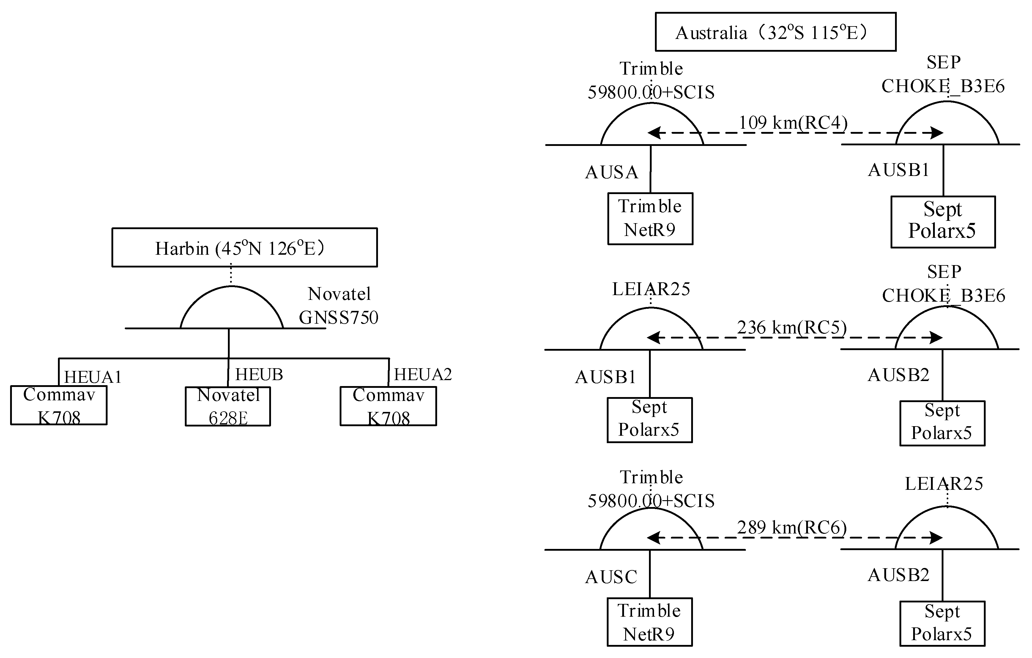
Since the available satellites with dual-frequency signals for GPS or BDS were sufficient, we took BDS and GPS with dual-frequency signals for an example to test the proposed method. A series of different baseline datasets were collected by different receiver types in two locations. The datasets were collected at intervals of 30 s. The satellite elevation mask was 10°. One location was Harbin, China, using Novatel 628 E and Comnav K708 receivers and a Novatel GNSS 750 antenna. Three groups of datasets were collected for 24 h from 0 a.m. to 24 p.m. at DOY 115 of 2019, denoted as Data 1. Another three groups of datasets from the receiver reboot test were collected for 2 days from DOY 147 to DOY 148 of 2019, denoted as Data 2. Note that all receivers use the same antenna. The last location was the open areas off the east coast of Australia, using Trimble NetR9 and Trimble 59800.00+SCIS antenna, POLARX5TR receivers and SEP CHOKE_B3E6 antenna, LEIAR25 antenna. Three long baseline datasets were collected for 24 h from 0:00 to 24:00 at DOY 115 of 2019, denoted as Data 3. Note that the receivers were installed in the indoor environment with a relatively constant temperature. It is reasonable to assume the hardware temperature does not affect the stability of the ISB. The detailed receiver and antenna setups are shown in Figure 1 and Table 2, in which RC represents receiver pairs. Note that although the receiver pair 5 (RC5) uses the same type of receiver, it uses different types of antennas.
All the methods were implemented at the single-epoch mode. The observation random model is designed by the elevation angle weighted model. The observation random model is the elevation weighted model:
where θ is the satellite elevation angle, σo is the standard deviation (STD) of the observations in the zenith direction. For the raw code, σo is 30 cm [7,16]. Meanwhile, the base station receiver will produce clock jump due to the adjustment of clock error, which will not only affect the observations, but also cause the discontinuity of pseudorange correction (PRC). Therefore, the receiver clock jump is detected and repaired. The positioning solutions in the following tests will not be affected by the receiver clock jump. Although the IF combination eliminates the effect of ionosphere delay on the DGNSS positioning model, the code noise is amplified. So, the multi-epoch accumulation method is used to reduce code noise for the IFLC and the proposed IFTC method.
3.1. ISB Analysis
The ISB from the proposed IFTC method is caused by different hardware delays in the satellite signal acquisition channel in the receiver, which is related with not only the receiver type and version, but also the state of the receiver, such as receiver reboot [2,32]. The time-domain stability of ISB with different types of receivers were firstly analyzed. Then, the ISB estimations from the L1TC and the L2TC methods were also analyzed to compare with the IFTC.
3.1.1. Stability Analysis
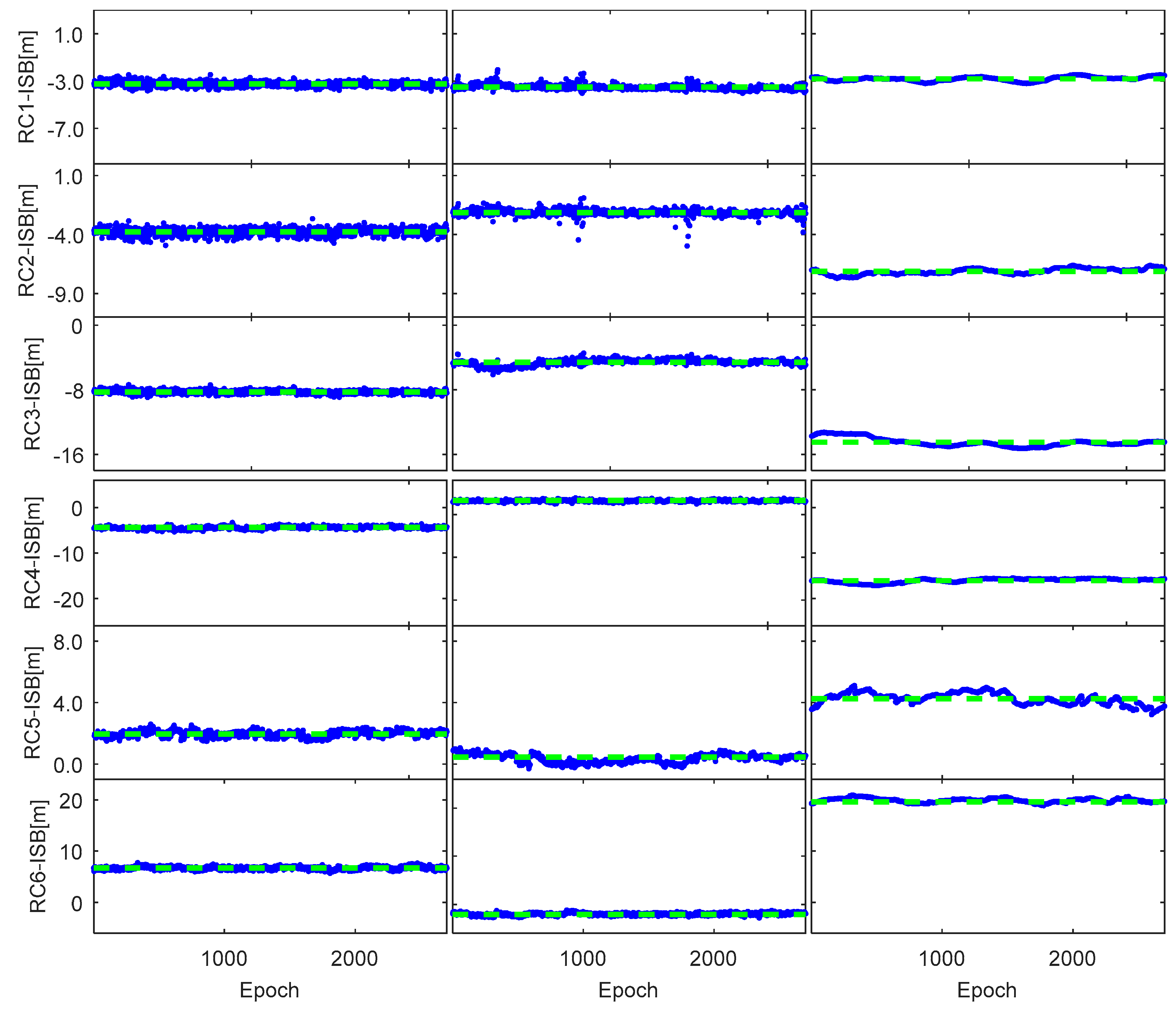
In order to study the stability of ISB from IFTC, we selected Data 1, Data 3 to confirm the stability of the ISB. Different types of receivers were used when Data 1, Data 3, was collected. The differential ISB model in TCDD was used to obtain the epoch-wise ISB in L1TC, L2TC, and IFTC methods, respectively. The ISB estimations are shown in Figure 2.
The mean and STD of the ISB estimations are shown in Table 3, where columns from left to right correspond to the ISB estimations from L1TC, L2TC, and IFTC methods, respectively. The columns from top to bottom are the ISB estimations for receiver pairs RC1, RC2, RC3, RC4, RC5, and RC6, respectively.
As seen from Figure 2 and Table 3, the mean absolute value of the receiver pair RC1 (HEUA1–HEUA2) ISB estimations (−3.24 m of the frequency L1-B1, −3.50 m of the frequency L2-B2) is minimum in Data 1, and the mean absolute value of the RC5 (HEUB– HEUA2) ISB estimations (1.94 m of the frequency L1-B1, 0.45 m of the frequency L2-B2) is minimum in Data 3. In Figure 1, the receiver type and version of the receiver pairs RC1 and RC5 are the same, but other receiver pairs are different. The mean absolute value of the receiver pair RC3 (HEUB–HEUA2) ISB estimations (8.26 m of the frequency L1-B1) in Data 1 is the maximum. The mean absolute value of the receiver pair RC6 (AUSC–AUSD) ISB estimations (6.67 m of the frequency L1-B1) in Data 3 is the maximum. It can be explained by the fact that the inconsistency of physical hardware from different receiver types will cause a relatively large value of the ISB [25]. Therefore, the ISB has a close relationship with receiver type and version.
The receiver pair RC2 and the receiver pair RC3 have the same receiver type and version and the same antennas, but the ISB estimations of them are different. The receiver pair RC4 and the receiver pair RC6 have the same receiver type and version except that the Sept Polarx5tr receiver has the different antennas, and the ISB estimations of them are also different. The finding indicates the ISB may differ for each receiver pair.
As seen from Figure 2 and Table 3, the STDs of the ISB estimations are almost all less than 0.3 m, and are therefore comparable to the STDs of code observational noise. Therefore, the ISB estimations from the L1TC, L2TC, and IFTC methods are very stable. It is reasonable to calibrate the ISB in the proposed IFTC method due to their time-invariant feature.
Theoretically, the ISB of the IF combination is a linear combination relationship between the ISB of the frequency L1-B1 and the ISB of the frequency L2-B2. The IF combination coefficient can be simplified as
where , is the coefficient of the IF combination simplified model. Theoretically, the ISB of the IF combination can be obtained by Equation (11), using the ISB estimations at the frequency L1-B1 and the frequency L2-B2 in a real test as shown in Table 4.
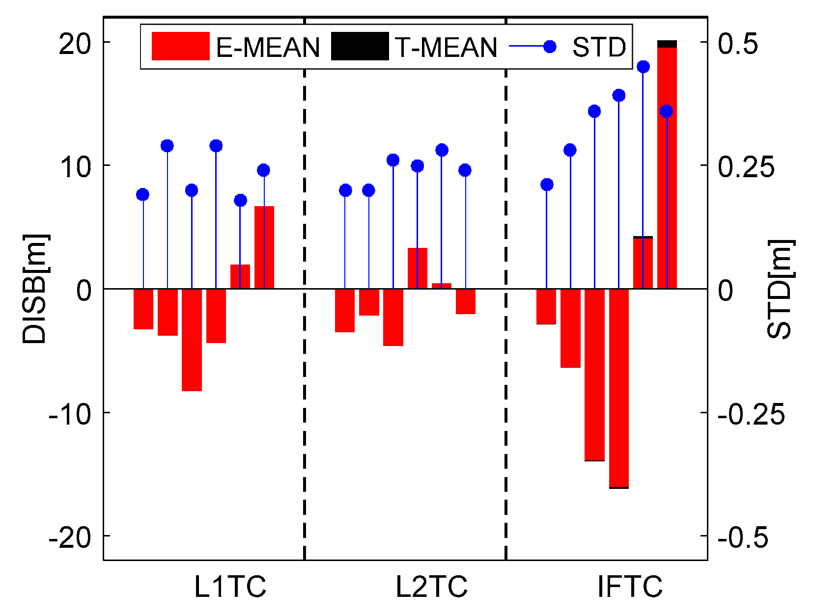
To manifest the difference between theoretical ISB estimations in Equation (11) and the estimated one in Equation (8), the means and STDs of the ISB estimations of the IF combination are compared in Figure 3.
As seen from Figure 3 and Table 4, the ISB estimations of the IF combination in real tests are less than the theoretical ISB of the IF combination, and particularly Data 3 in long baseline cases has obvious ionospheric residual in the DGNSS model. It can be explained by the fact that the IF combination observations model can eliminate the effect of ionosphere delay on ISB estimations in real tests. In contrast, the single frequency observations model cannot eliminate the effect of ionosphere delay on ISB estimations, especially in long baseline cases. Theoretically, the IF-based ISB estimations obtained by the ISB of the frequency L1-B1 and the frequency L2-B2 are still affected by the ionosphere delay residual. Therefore, the ISB from the proposed IFTC method is reasonable to be calibrated by the IF-based ISB estimations in real test.
Table 5 shows the repeatability of the ISB estimated in the single-epoch solution and in the multi-epoch solution for Data 1 and Data 3. Table 5 shows that the mean values of the ISB estimations from the multi-epoch solution are consistent with those of the single-epoch solution. The standard deviations of the single-epoch results for the three receiver pairs are also at the level of a few decimeters. The standard deviation of the ISB becomes smaller with increasing epochs. The precision of the ISB for some receiver pairs can reach a few centimeters within 50 epochs. In this case, the sizes of the ISB in the IFTC method for RC4, RC5, and RC6 are −16.01 m, 4.15 m, and 19.62 m, respectively [2].
3.1.2. Effect of Receiver Reboot
Previous studies have shown that the stability of the ISB will be affected by receiver reboot and the temperature fluctuation of the receiver hardware [31,32]. The test datasets were collected under an indoor environment with nearly constant temperature, and the influence of temperature fluctuation will not be considered. Herein, we only tested whether or not the stability of the ISB are affected by the receiver reboot. If the ISBs change when receivers are rebooted, the calibration of the ISB cannot be used to correct the IFTC DGNSS model. In such cases, the ISBs can only be re-estimated and modeled during a continuous observation period in real-time cases.
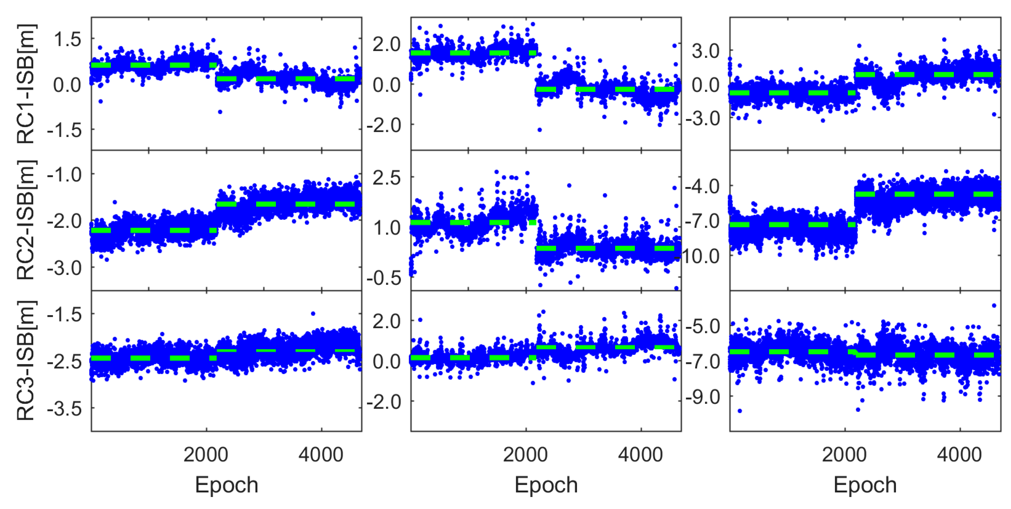
We selected Data 2 to clarify the ISB feature with the state of receiver reboot. The ISB of three tightly coupled methods (L1TC, L2TC, IFTC) were estimated by the TCDD model. The estimations of epoch-wise ISB are shown in Figure 4. The statistical characteristics of the corresponding mean and STD of ISB are shown in Table 6.
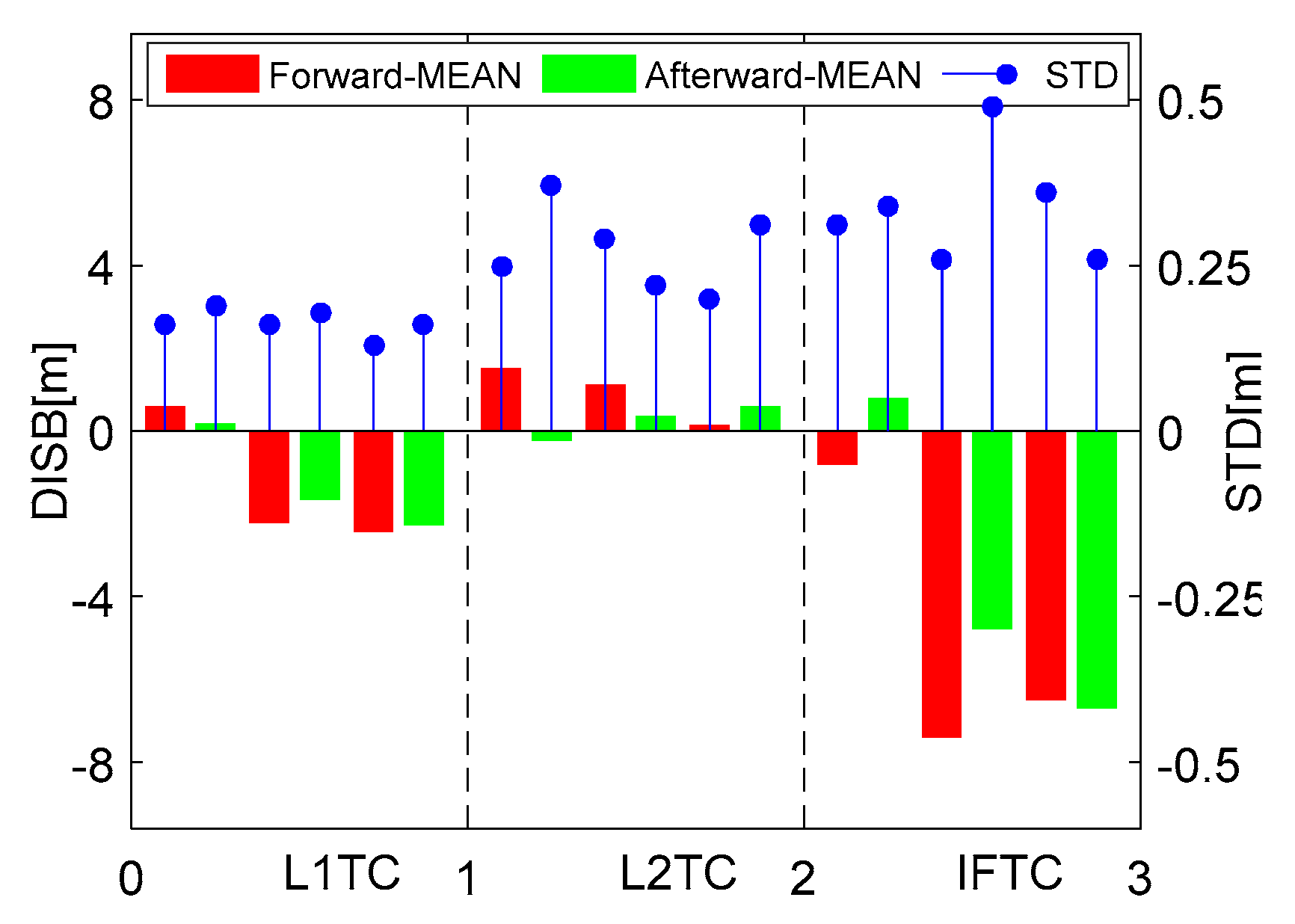
For the receiver pair RC2 (HEUB–HEUA1) with its different receiver types and versions, as far as the L2TC method and the IFTC method are concerned, a remarkable change in the ISB estimations is observed when the receivers are rebooted. A remarkable change of ISB estimations is also present for the receiver pair RC3 (HEUB–HEUA2) with different receiver types and versions at the frequency L2-B2, when the receivers are rebooted. For the receiver pair RC1 (HEUA1–HEUA2) with the same receiver type and version, the ISB estimations also jump when the receivers are rebooted. Table 6 shows that the mean of the receiver pair RC1 (HEUA1–HEUA2) ISB estimations changes from 0.60 m to 0.18 m in the L1TC method, and from −0.82 m to 0.80 m in the IFTC method. The means of RC2 and RC3 ISB estimations also change by the L1TC, L2TC, and IFTC methods. It suggests that whether the receiver type and version is the same or not, the ISB estimations have obvious changes when receivers are rebooted.
To manifest the difference between the difference receiver pairs, the means and STDs of ISB are compared in Figure 5. It can be seen that the STD of receiver pair RC2 (HEUB-HEUA1) ISB estimations is 0.49 m; the maximum among the three receiver pairs is not more than 0.5 m and is comparable to the STDs of code observational noise after the receivers are rebooted. It suggests that the ISB still has a time-invariant feature after the receivers were rebooted. The ISB can be re-calibrated in the IFTC method in the presence of receiver reboot to prevent the biased ISB calibration from affecting positioning accuracy.
3.2. Positioning Performance Analysis
In order to test the proposed IFTC method, the L1LC, DFTC, and IFLC methods in the long baseline case, Data 3 were used for positioning performance comparison and analysis. The multi-epoch solution method was adopted to suppress observation noise. The ISB has a time-invariant feature and can be calibrated. Fortunately, the centimeter-level accuracy of the ISB can be obtained by pre-estimation among several epochs. The mean of ISB estimations, obtained by solution initial 50 epochs, is used as the ISB calibration of the tightly coupled method. In addition, to reveal the effectiveness of tightly coupled positioning under the satellite deprived environment, the positioning performance of different methods are evaluated by varying the cutoff elevation angles as 15°, 25°, 35°, and 45°, respectively.
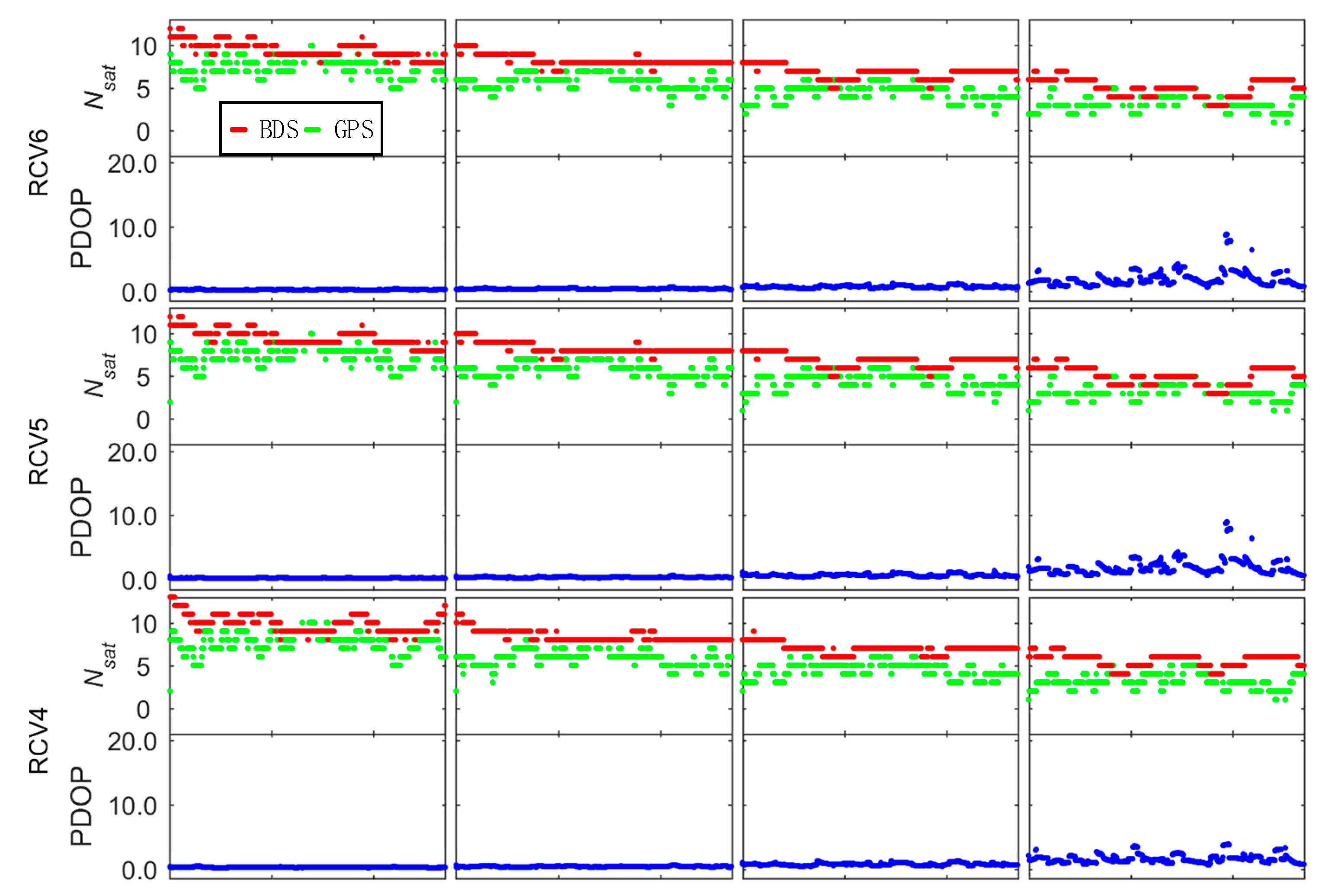
The position dilution of precision (PDOP) and the satellite number with different cutoff elevation angles of the receiver pairs RC4, RC5, and RC6 are shown in Figure 6. The mean of Nsat and PDOP with the different cutoff elevation angles is summarized in Table 7. Note that the means of Nsat are calculated by the rounding method.
In Figure 6 and Table 7, it can be found that when the cutoff elevation angle is set to less than 25°, the receiver pairs RC4, RC5, and RC6 can observe more than 13 satellites for GPS and BDS, and the PDOPs are less than 1. When the cutoff elevation angle is set to 35°, the number of satellites observed by the receiver pairs RC4, RC5, and RC6 all are 10. The PDOP of receiver pair RC6 is 2.7. When the cutoff elevation angle is set to 45°, the receiver pair RC6 has the minimum number of satellites and the maximum PDOP. The greater the cutoff elevation angle and baseline, the fewer the consensus satellites and the bigger PDOP. For satellite-deprived environments, the proposed IFTC method can improve the redundancy of the DGNSS model, which is beneficial for enhancing positioning performance.
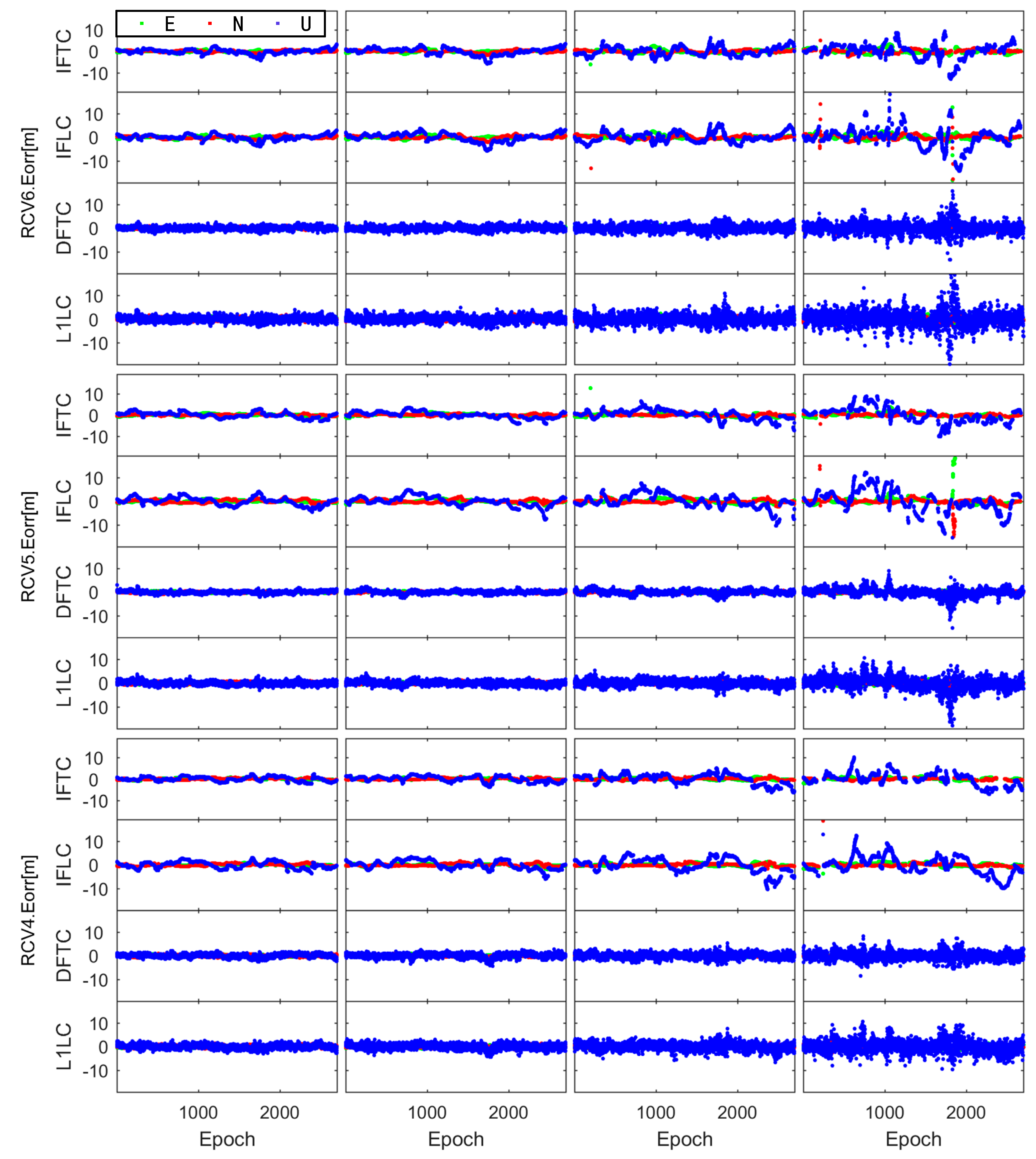
The positioning errors of the L1LC, DFTC, IFLC, and IFTC methods are shown in Figure 7. The root mean square (RMS) of positioning error with different cutoff elevation angles is summarized in Table 8.
In Figure 7 and Table 8, it can be found that when the cutoff elevation angle is set to less than 25°, the L1TC, DFTC, IFLC, and IFTC methods achieve comparable positioning accuracy for the receiver pairs RC4, RC5, and RC6. Note that the positioning accuracy of the proposed IFTC method is slightly better than that of other methods. The results indicate that the proposed IFTC method is comparable to the traditional IFLC method given sufficient available satellites. When the cutoff elevation is increased from 25° to 45°, Figure 7 shows the positioning performance of the traditional IFLC method is worse than the proposed IFTC method. At the vertical direction, the proposed IFTC method positioning accuracy is increased by 19% (RC4), 30% (RC5), and 21% (RC6), compared with the L1LC method. Compared with the IFLC method, the proposed IFTC method positioning accuracy is increased by 31% (RC4), 14% (RC5), and 7% (RC6), at the vertical direction. The proposed IFTC method positioning accuracy is increased by 31% (RC4), 24% (RC5), and 28% (RC6), compared with the DFLC method at the vertical direction. The results indicate that the IFTC method eliminates the influence of ionospheric residual on positioning performances, and obtains higher model strength than the loose combination, which is significant under the satellite-deprived environment. To sum up, the proposed IFTC DGNSS method with ISB calibration can maintain better positioning performance, particularly under satellite-deprived environments.
Positioning continuity is another important metric reflecting positioning performances [13,14,16,36]. Positioning continuity with different cutoff elevation angles is shown in Table 9. Note that positioning continuity is the ratio of positioning epochs and total positioning epochs.
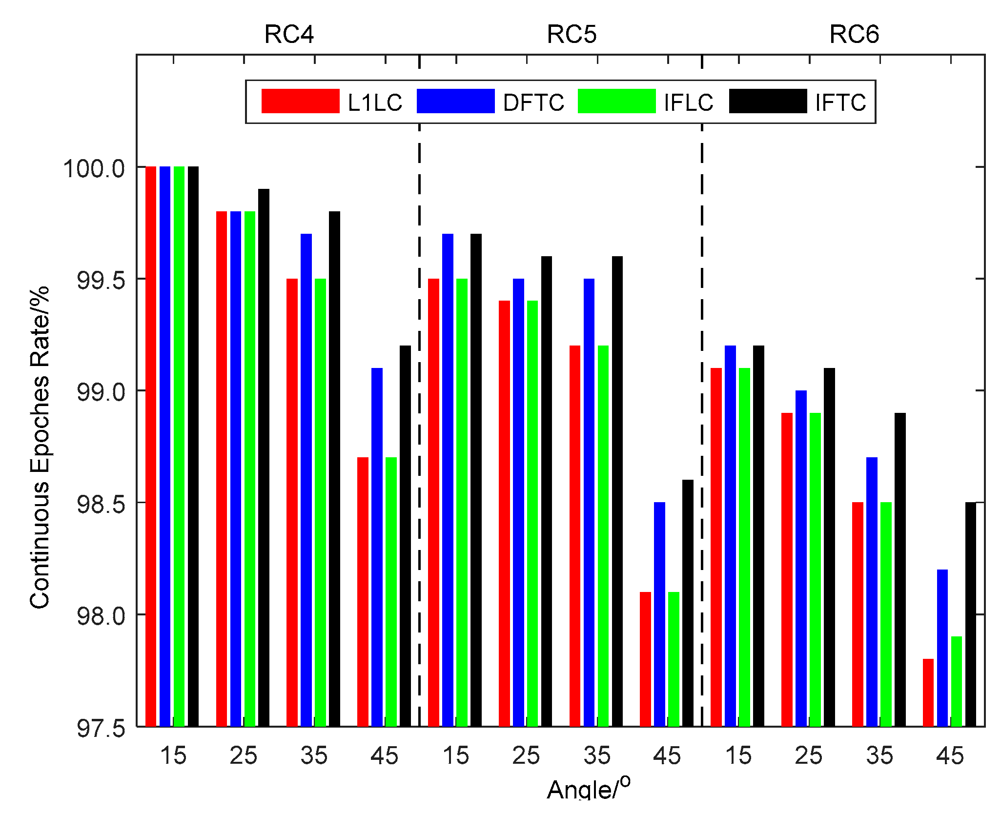
To manifest the difference between different receiver pairs, the positioning continuity rates are compared in Figure 8.
When the cutoff elevation angles are less than 25°, as shown in Figure 8 and Table 9, the positioning continuity rates of the L1TC, DFTC, IFLC, and IFTC methods are above 99% for the receiver pairs RC4, RC5, and RC6. When the cutoff elevation is increased from 25° to 45° for the three receiver pairs, Pc of the IFTC method is also greater than it is in the other methods. Taking the receiver pair RC6 as an example, when compared with the L1TC and IFLC methods, the positioning continuity of the IFTC method is improved by 0.7% and 0.6%, respectively, and the discontinuity epochs are reduced by about 32% and 27%, respectively. As shown in Table 1, the DFTC method has about twice the number of observation redundancies as the IFTC method does, but Pc of the DFTC method is also less than it is in the IFTC method. This indicates that the ionospheric residual, rather than the redundancy, is the dominant factor affecting the positioning continuity of the DGNSS model in the long baseline case. According to Figure 8 and Table 9, when the cutoff elevation is 45°, the continuity rates of receiver pair RC5 and the receiver pair RC6 are reduced, compared with receiver pair RC4. This is due to the decrease of common-in-view satellites with the baseline length increasing, resulting in the decrease of positioning continuity. Compared with other methods, the proposed IFTC method has the best continuity for the greatest model strength and for eliminating the influence of ionospheric residual.
Generally, the proposed IFTC DGNSS model can obtain meter-level or even decimeter-level accuracy and the best positioning in real-time positioning. Figure 7 and Figure 8, and Table 8 and Table 9 show that for the receiver pair RC4 with a baseline 109 km using the proposed IFTC method, the horizontal accuracy is about 1 m, the positioning continuity rate is more than 99%, and the vertical accuracy is more than 1.0 m. For the receiver pair RC5 with a baseline 236 km by the IFTC methods, the eastern and northern accuracies can be obtained within 1.0 m and positioning continuity rate more than 98%, while the vertical one does exceed 2.0 m. For the receiver pair RC6 with a baseline 289 km by the IFTC methods, the eastern and northern accuracies can be obtained at more than 1.0 m; the vertical one does exceed 2.0 m, and the positioning continuity rate is less than 97%. It suggests that the proposed IFTC method can obtain the best balance between positioning accuracy and positioning continuity compared with other methods. It is because the proposed IFTC method not only improves model strength, but also eliminates the influence of ionospheric residual. However, due to the increase of the baseline, the number of common-in-view satellites decreases significantly and the ionospheric residual increases. When the baseline exceeds 240 km in real-time positioning, the proposed IFTC method cannot obtain the meter-level and cannot meet the RBN-DGNSS application positioning requirements.
4. Conclusions
In order to improve the positioning accuracy and continuity performance of the RBN-DGNSS under satellite-deprived environments, the ionosphere-free inter-frequency tightly coupled method DGNSS with ISB calibration, which is compatible with the traditional RBN base station implementation, is proposed. The proposed method improves the model strength by inter-system combination and eliminates the effect of ionosphere delay by the inter-frequency combination. The proposed tightly coupled method is pre-calibrated by the differential ISB estimated from the tightly coupled double difference observation model.
The proposed method is tested by several datasets collected under different baselines with various types of receivers. The results show that the ISB is sufficiently stable and closely related with the receiver types, which can be calibrated by the pre-estimation method. In addition, the ISB needs to be re-calibrated when the receivers are rebooted. In the experiment, the cutoff elevation was artificially set to simulate the restricted conditions of satellite signal reception. It has shown that the proposed IFTC method is comparable to the traditional IFLC method when the cutoff elevation angle is less than 25°. When the cutoff elevation angle is increased to 45°, the positioning accuracy of the proposed method can be improved by 31% at the vertical direction and the discontinuity epoch can be reduced by 32%, compared with the traditional ionosphere delay free loosely coupled DGNSS. It is because the proposed IFTC method not only improves model strength, but also eliminates the influence of ionospheric residual. However, with the baseline increasing, the number of common-in-view satellites decreases significantly and the ionospheric residual increases. The proposed IFTC method obtains the meter-level or even decimeter-level horizontal accuracy when the baseline is only within 240 km.
Author Contributions
Conceptualization, J.C., C.J. (Chao Jiang), L.L. and C.J. (Chun Jia); Data curation, C.J. (Chao Jiang), J.L.; Investigation, C.J. (Chao Jiang), L.L. and C.J. (Chun Jia); Methodology, C.J. (Chao Jiang) and L.L.; Software, C.J. (Chao Jiang); Supervision, L.L.; Validation, C.J. (Chao Jiang), C.J. (Chun Jia) and B.Q.; Writing—original draft, C.J. (Chao Jiang) and L.L.; Writing—review and editing, J.C., C.J. (Chao Jiang), L.L., C.J. (Chun Jia), B.Q. and J.L. All authors have read and agreed to the published version of the manuscript.
Funding
This research was jointly funded by the National Natural Science Foundation of China (Nos. 61773132, 61633008, 61803115), the National Key Research and Development Program (No. 2017YFE0131400), the 145 High-tech Ship Innovation Project sponsored by Chinese Ministry of Industry and Information Technology, the Heilongjiang Province Research Science Fund for Excellent Young Scholars (No. YQ2020F009), the Heilongjiang Province Research Science Fund for Distinguished Young Scholars (No. JC2018019), and the Fundamental Research Funds for Central Universities (Nos. 3072019CF0401, 3072020CFJ0402, 3072020CFT0403).
Acknowledgments
The authors acknowledge the International GNSS Service (IGS) for providing the data.
Conflicts of Interest
The authors declare no conflict of interest.
References
- Kremer, G.T.; Kalafus, R.M.; Loomis, P.V.W.; Reynolds, J.C. The Effect of Selective Availability on Differential GPS Corrections. Navigation 1990, 37, 39–52. [Google Scholar] [CrossRef]
- Liu, H.; Shu, N.; Xu, L.; Qian, C.; Zhang, R.; Zhang, M. Accounting for Inter-System Bias in DGNSS Positioning with GPS/GLONASS/BDS/Galileo. J. Navig. 2017, 70, 686–698. [Google Scholar] [CrossRef]
- Technical Requirements of Differential Global Positioning System; GB/T 17424-2009; GNSS&LBS Association of China: Beijing, China, 2009.
- Li, N.; Zhao, L.; Li, L.; Jia, C. Integrity monitoring of high-accuracy GNSS-based attitude determination. GPS Solut. 2018, 22, 120. [Google Scholar] [CrossRef]
- Cai, C.; Gao, Y. A Combined GPS/GLONASS Navigation Algorithm for use with Limited Satellite Visibility. J. Navig. 2009, 62, 671–685. [Google Scholar] [CrossRef]
- Jia, C.; Li, L.; Lu, R. BDS triple-frequency tightly coupled short-baseline RTK method by calibrating the between-receiver inter frequency biases. Sci. Sin. Terrae China 2020, 50, 1–14. [Google Scholar]
- Li, L.; Li, Z.; Yuan, H.; Wang, L.; Hou, Y. Integrity monitoring-based ratio test for GNSS integer ambiguity validation. GPS Solut. 2016, 20, 573–585. [Google Scholar] [CrossRef] [Green Version]
- Li, L.; Jia, C.; Zhao, L.; Yang, F.; Li, Z. Integrity monitoring-based ambiguity validation for triple-carrier ambiguity resolution. GPS Solut. 2016, 21, 797–810. [Google Scholar] [CrossRef]
- Li, T.; Zhang, H.; Niu, X.; Gao, Z. Tightly-Coupled Integration of Multi-GNSS Single-Frequency RTK and MEMS-IMU for Enhanced Positioning Performance. Sensors 2017, 17, 2462. [Google Scholar] [CrossRef] [Green Version]
- Odijk, D.; Teunissen, P.J.G. Characterization of between-receiver GPS-Galileo inter-system biases and their effect on mixed ambiguity resolution. GPS Solut. 2012, 17, 521–533. [Google Scholar] [CrossRef]
- Torre, A.D.; Caporali, A. An analysis of intersystem biases for multi-GNSS positioning. GPS Solut. 2014, 19, 297–307. [Google Scholar] [CrossRef]
- Li, G.; Geng, J.; Guo, J.; Zhou, S.; Lin, S. GPS + Galileo tightly combined RTK positioning for medium-to-long baselines based on partial ambiguity resolution. J. Glob. Position. Syst. 2018, 16, 3. [Google Scholar] [CrossRef] [Green Version]
- Li, L.; Quddus, M.; Ison, S.; Zhao, L. Multiple reference consistency check for LAAS: A novel position domain approach. GPS Solut. 2011, 16, 209–220. [Google Scholar] [CrossRef] [Green Version]
- Li, L.; Wang, H.; Jia, C.; Zhao, L.; Zhao, Y. Integrity and continuity allocation for the RAIM with multiple constellations. GPS Solut. 2017, 21, 1503–1513. [Google Scholar] [CrossRef]
- Odolinski, R.; Teunissen, P.J.G.; Odijk, D. Combined BDS, Galileo, QZSS and GPS single-frequency RTK. GPS Solut. 2015, 19, 151–163. [Google Scholar] [CrossRef]
- Li, L.; Shi, H.; Jia, C.; Cheng, J.; Li, H.; Zhao, L. Position-domain integrity risk-based ambiguity validation for the integer bootstrap estimator. GPS Solut. 2018, 22, 39. [Google Scholar] [CrossRef]
- Xi, R.; Chen, Q.; Meng, X.; Jiang, W.; An, X.; He, Q. A Multi-GNSS Differential Phase Kinematic Post-Processing Method. Remote Sens. 2020, 12, 2727. [Google Scholar] [CrossRef]
- Odijk, D.; Teunissen, P.J.; Huisman, L. First results of mixed GPS+GIOVE single-frequency RTK in Australia. J. Spat. Sci. 2012, 57, 3–18. [Google Scholar] [CrossRef]
- Zeng, A.; Yang, Y.; Ming, F.; Jing, Y. BDS–GPS inter-system bias of code observation and its preliminary analysis. GPS Solut. 2017, 48, 149–1581. [Google Scholar] [CrossRef]
- Zhang, B.; Teunissen, P.J.G. Characterization of multi-GNSS between-receiver differential code biases using zero and short baselines. Sci. Bull. 2015, 60, 1840–1849. [Google Scholar] [CrossRef] [Green Version]
- Zhang, X.; Wu, M.; Liu, W. Model and Performance Analysis of Tightly Combined BeiDou B2 and Galileo E5b Relative Positioning for Short Baseline. Acta Geod. Cartograph. Sin. 2016, 45, 1–11. [Google Scholar]
- Li, B.; Verhagen, S.; Teunissen, P.J. Robustness of GNSS integer ambiguity resolution in the presence of atmospheric biases. GPS Solut. 2013, 18, 283–296. [Google Scholar] [CrossRef]
- Paziewski, J.; Wielgosz, P. Accounting for Galileo–GPS inter-system biases in precise satellite positioning. J. Geod. 2015, 89, 81–93. [Google Scholar] [CrossRef] [Green Version]
- Li, H.; Xiao, J.; Zhu, W. Investigation and Validation of the Time-Varying Characteristic for the GPS Differential Code Bias. Remote Sens. 2019, 11, 428. [Google Scholar] [CrossRef] [Green Version]
- Kubo, N.; Tokura, H.; Pullen, S. Mixed GPS–BeiDou RTK with inter-systems bias estimation aided by CSAC. GPS Solut. 2017, 22, 5. [Google Scholar] [CrossRef]
- Zhao, W.; Chen, H.; Gao, Y.; Jiang, W.; Liu, X. Evaluation of Inter-System Bias between BDS-2 and BDS-3 Satellites and Its Impact on Precise Point Positioning. Remote Sens. 2020, 12, 2185. [Google Scholar] [CrossRef]
- Odijk, D. Weighting Ionospheric Corrections to Improve Fast GPS Positioning Over Medium Distances. In Proceedings of the ION GNSS 2000, Salt Lake City, UT, USA, 19–22 September 2000; pp. 1113–1123. [Google Scholar]
- Takasu, T.; Yasuda, A. Kalman-Filter-Based Integer Ambiguity Resolution Strategy for Long-Baseline RTK with Ionosphere and Troposphere Estimation. In Proceedings of the ION GNSS 2010, Portland, OR, USA, 1–24 September 2010; pp. 161–171. [Google Scholar]
- Jia, C.; Zhao, L.; Li, L.; Cheng, J.; Li, H. Ionosphere-free Multi-carrier Ambiguity Resolution Method Based on Ambiguity Linear Constraints. Acta Geod. Cartograph. Sin. 2018, 47, 930–939. [Google Scholar]
- Su, K.; Jin, S.; Hoque, M.M. Evaluation of Ionospheric Delay Effects on Multi-GNSS Positioning Performance. Remote Sens. 2019, 11, 171. [Google Scholar] [CrossRef] [Green Version]
- Wu, M.; Liu, W.; Wu, R.; Zhang, X. Tightly combined GPS/Galileo RTK for short and long baselines: Model and performance analysis. Adv. Space Res. 2019, 63, 2003–2020. [Google Scholar] [CrossRef]
- Wu, M.; Zhang, X.; Liu, W.; Wu, R.; Zhang, R.; Le, Y.; Wu, Y. Influencing Factors of GNSS Differential Inter-System Bias and Performance Assessment of Tightly Combined GPS, Galileo, and QZSS Relative Positioning for Short Baseline. J. Navig. 2018, 72, 965–986. [Google Scholar] [CrossRef]
- Liu, Z.; Yue, D.; Huang, Z.; Chen, J. Performance of real-time undifferenced precise positioning assisted by remote IGS multi-GNSS stations. GPS Solut. 2020, 24, 1–14. [Google Scholar] [CrossRef]
- Schüler, T.; Diessongo, H.; Poku-Gyamfi, Y. Precise ionosphere-free single-frequency GNSS positioning. GPS Solut. 2010, 15, 139–147. [Google Scholar] [CrossRef]
- Odijk, D.; Nadarajah, N.; Zaminpardaz, S.; Teunissen, P.J.G. GPS, Galileo, QZSS and IRNSS differential ISBs: Estimation and application. GPS Solut. 2016, 21, 439–450. [Google Scholar] [CrossRef]
- Zhao, L.; Zhang, J.; Li, L.; Yang, F.; Liu, X. Position-Domain Non-Gaussian Error Overbounding for ARAIM. Remote Sens. 2020, 12, 1992. [Google Scholar] [CrossRef]
Figure 1.
Receiver and antenna setups.

Figure 2.
Inter-system bias (ISB) estimations from different tightly coupled methods. The columns from left to right correspond to L1TC, L2TC, and the IF-based tightly coupled (IFTC) method, respectively. The ISB estimations are represented by blue and the mean of the ISB estimations is represented by green. The columns from top to bottom are the ISB estimations of receiver pairs RC1, RC2, RC3, RC4, RC5, and RC6.

Figure 3.
Mean and standard deviation of ISB estimations. The columns from left to right correspond to the L1TC, L2TC, and the IFTC method, respectively. In the L1TC part, the columns from left to right are the ISB estimations of receiver pairs RC1, RC2, RC3, RC4, RC5, and RC6, respectively. The L2TC part and the IFTC part are also the same as the L1TC part. The mean of ISB estimations in the real test is represented by the red bar, denoted as E-MEAN. The mean of the theoretical ISB estimations is also represented by the red bar, denoted as T-MEAN. The STD of the ISB estimations in real test are represented by the blue stem.

Figure 4.
ISB estimations in receiver reboot experiments. The columns from left to right are the L1TC, L2TC, and the IFTC method, respectively. The columns from top to bottom are the ISB estimations of receiver pairs RC1, RC2, and RC3, respectively. Note that the ISB estimations are represented by blue points and the mean of ISB estimations is represented by green points.

Figure 5.
Mean and standard deviation of ISB estimations from the receiver reboot test. The columns from left to right correspond to the L1TC, L2TC, and the IFTC method, respectively. In the L1TC part, the columns from left to right are the ISB estimations of the receiver pairs RC1, RC2, and RC3, respectively. The other parts are also the same as the L1TC part. The mean of the ISB estimations are represented by a red bar before the receivers are rebooted and by a green bar after the receivers are rebooted, and the STDs of the ISB are represented by blue stems.

Figure 6.
PDOP and satellite number with different cutoff elevation angles. Nsat represents the number of visible satellites, and PDOP represents the position dilution of precision of BDS and GPS satellites. Note that eastern errors are represented by green points, northern errors are represented by red points, and vertical errors are represented by blue points. The rows from top to bottom are satellite number and the PDOP of RC6, RC5, and RC4. The columns from left to right correspond to the different cutoff elevation angles (15°, 25°, 35°, and 45°).

Figure 7.
Positioning errors with different cutoff elevation angles (m). The rows from top to bottom are positioning errors of the receiver pairs RC4, RC5, and RC6 from the L1LC, DFTC IFLC, and IFTC methods. Note that eastern errors are represented by green points, northern errors are represented by red points, and vertical errors are represented by blue points. The columns from left to right correspond to different cutoff elevation angles (15°, 25°, 35°, and 45°).

Figure 8.
Positioning continuity epochs results with different cutoff elevation angles. The columns from left to right correspond to receiver pair RC4, RC5 and RC6, respectively. In the L1TC part, the columns from left to right are the cutoff elevation angles 15°, 25°, 35°, and 45°, respectively. The other parts are also the same as L1TC part. Note that the Pc of L1TC, DFTC, IFLC, and IFTC are represented by red bars, blue bars, green bars, and black bars.


Table 1.
Redundancy of different methods.
| Model | # of Obs | #Parameters | #Redundancy |
|---|---|---|---|
| L1LC | fG·MG + fB·MB | 5 | fG·(MG − 1) + fB·(MB − 1) − 3 |
| L1TC (pre-calibrated ISB) | fG·MG + fB·MB | 4 | fG·MG + fB·(MB − 1) − 3 |
| L2LC | fG·MG + fB·MB | 5 | fG·(MG− 1) + fB·(MB − 1) − 3 |
| L2TC (pre-calibrated ISB) | fG·MG + fB·MB | 4 | fG·MG + fB·(MB − 1) − 3 |
| DFLC | 2 (fG·MG + fB·MB) | 7 | 2·fG·(MG− 1) + 2 fB·(MB − 1) − 3 |
| DFTC (pre-calibrated ISB) | 2 (fG·MG + fB·MB) | 5 | 2 fGMG + 2 fB·(MB − 1) − 3 |
| IFLC | fG·MG + fB·MB | 5 | fG·(MG − 1) + fB·(MB − 1) − 3 |
| IFTC (pre-calibrated ISB) | fG·MG + fB·MB | 4 | fG·MG + fB·MB − 4 |
Table 2.
Baseline setups.
| Data | Number | RC Pairs | Baseline |
|---|---|---|---|
| Data 1/Data 2 | RC1 | K708_01 (HEUA1)–K708_02 (HEUA2) | 0 km |
| RC2 | 628E (HEUB)–K708_01 (HEUA1) | 0 km | |
| RC3 | 628E (HEUB)–K708_02 (HEUA2) | 0 km | |
| Data 3 | RC4 | Trimble NetR9 (AUSA)–Sept Polarx5tr (AUSB1) | 109 km |
| RC5 | Sept Polarx5tr (AUSB1)–Sept Polarx5tr (AUSB2) | 236 km | |
| RC6 | Trimble NetR9 (AUSC)–Sept Polarx5tr (AUSB2) | 289 km |
Table 3.
Statistics of the ISB from different tightly coupled methods (m).
| Data | RC Pair | L1TC | L2TC | IFTC | |||
|---|---|---|---|---|---|---|---|
| Mean | STD | Mean | STD | Mean | STD | ||
| Data 1 | RC1: HEUA1–HEUA2 | −3.24 | 0.19 | −3.50 | 0.20 | −2.81 | 0.21 |
| RC2: HEUB–HEUA1 | −3.78 | 0.29 | −2.14 | 0.20 | −6.30 | 0.28 | |
| RC3: HEUB–HEUA2 | −8.26 | 0.20 | −4.61 | 0.26 | −13.89 | 0.36 | |
| Data 3 | RC4: AUSA–AUSB | −4.36 | 0.29 | 3.29 | 0.25 | −16.01 | 0.32 |
| RC5: AUSA–AUSC | 1.94 | 0.18 | 0.45 | 0.28 | 4.15 | 0.45 | |
| RC6: AUSC–AUSD | 6.67 | 0.24 | −2.02 | 0.24 | 19.62 | 0.36 | |
Table 4.
The mean of theoretical ISB value.
| RC Pair | Data 1 | Data 3 | ||||
|---|---|---|---|---|---|---|
| RC1 | RC2 | RC3 | RC4 | RC5 | RC6 | |
| Mean | −2.83 | −6.31 | −13.90 | −16.18 | 4.26 | 20.10 |
Table 5.
Statistics of ISB estimations with different initial epochs (m).
| Mode | RC Pairs | 1 Epoch | 20 Epochs | 50 Epochs | |||
|---|---|---|---|---|---|---|---|
| Mean | STD | Mean | STD | Mean | STD | ||
| L1TC | RC4: AUSA–AUSB | −4.35 | 0.33 | −4.36 | 0.30 | −4.36 | 0.28 |
| RC5: AUSA–AUSC | 1.94 | 0.23 | 1.90 | 0.19 | 1.89 | 0.18 | |
| RC6: AUSD–AUSC | 6.67 | 0.28 | 6.65 | 0.24 | 6.66 | 0.25 | |
| L2TC | RC4: AUSA–AUSB | 3.29 | 0.26 | 3.12 | 0.24 | 3.18 | 0.23 |
| RC5: AUSA–AUSC | 0.45 | 0.28 | 0.42 | 0.27 | 0.44 | 0.26 | |
| RC6: AUSD–AUSC | −2.02 | 0.24 | −2.01 | 0.34 | −1.98 | 0.25 | |
| IFTC | RC4: AUSA–AUSB | −16.01 | 0.39 | −16.87 | 0.35 | −15.98 | 0.30 |
| RC5: AUSA–AUSC | 4.15 | 0.38 | 4.19 | 0.36 | 4.18 | 0.34 | |
| RC6: AUSD–AUSC | 19.62 | 0.36 | 19.58 | 0.33 | 19.46 | 0.29 | |
Table 6.
Statistics of ISB estimations in receiver reboot test (m).
| Reboot | RC Pair | L1TC | L2TC | IFTC | |||
|---|---|---|---|---|---|---|---|
| Mean | STD | Mean | STD | Mean | STD | ||
| Forward | RC1: HEUA1–HEUA2 | 0.60 | 0.16 | 1.52 | 0.25 | −0.82 | 0.36 |
| RC2: HEUB–HEUA1 | −2.22 | 0.16 | 1.12 | 0.29 | −7.39 | 0.21 | |
| RC3: HEUB–HEUA2 | −2.44 | 0.13 | 0.14 | 0.20 | −6.50 | 0.36 | |
| Afterward | RC1: HEUA1–HEUA2 | 0.18 | 0.19 | −0.23 | 0.37 | 0.80 | 0.34 |
| RC2: HEUB–HEUA1 | −1.67 | 0.18 | 0.36 | 0.22 | −4.78 | 0.49 | |
| RC3: HEUB–HEUA2 | −2.27 | 0.16 | 0.59 | 0.31 | −6.69 | 0.26 | |
Table 7.
Mean of the PDOP and satellite number with different cutoff elevation angles.
| RCPairs | 15° | 25° | 35° | 45° | ||||||||
|---|---|---|---|---|---|---|---|---|---|---|---|---|
| GPS | BDS | PDOP | GPS | BDS | PDOP | GPS | BDS | PDOP | GPS | BDS | PDOP | |
| RC4 | 7 | 10 | 0.1 | 5 | 8 | 0.8 | 4 | 6 | 2.4 | 3 | 5 | 2.0 |
| RC5 | 7 | 9 | 0.1 | 5 | 8 | 0.9 | 4 | 6 | 2.5 | 3 | 4 | 3.2 |
| RC6 | 7 | 9 | 0.2 | 5 | 8 | 0.9 | 4 | 6 | 2.7 | 3 | 4 | 4.5 |
Table 8.
Error root mean square (RMS) of positioning results with different cutoff elevation angles (m).
Table 8.
Error root mean square (RMS) of positioning results with different cutoff elevation angles (m).
| RC Pairs | Model | 15° | 25° | 35° | 45° | ||||||||
|---|---|---|---|---|---|---|---|---|---|---|---|---|---|
| E | N | U | E | N | U | E | N | U | E | N | U | ||
| RC4 | L1LC | 0.35 | 0.41 | 1.01 | 0.35 | 0.42 | 1.01 | 0.45 | 0.56 | 1.27 | 0.69 | 0.66 | 1.38 |
| DFTC | 0.31 | 0.32 | 1.02 | 0.30 | 0.33 | 0.95 | 0.48 | 0.55 | 1.20 | 0.56 | 0.63 | 1.34 | |
| IFLC | 0.25 | 0.26 | 0.94 | 0.24 | 0.24 | 0.93 | 0.32 | 0.39 | 0.99 | 0.44 | 0.56 | 1.25 | |
| IFTC | 0.24 | 0.19 | 0.92 | 0.23 | 0.19 | 0.92 | 0.36 | 0.33 | 0.95 | 0.40 | 0.50 | 1.12 | |
| RC5 | L1LC | 0.89 | 0.87 | 1.35 | 0.90 | 0.86 | 1.37 | 0.96 | 0.98 | 1.58 | 1.12 | 1.10 | 2.49 |
| DFTC | 0.86 | 0.79 | 1.34 | 0.87 | 0.76 | 1.35 | 0.95 | 0.96 | 1.46 | 1.09 | 1.08 | 1.99 | |
| IFLC | 0.74 | 0.73 | 1.28 | 0.74 | 0.73 | 1.29 | 0.82 | 0.81 | 1.38 | 1.01 | 1.05 | 1.89 | |
| IFTC | 0.73 | 0.72 | 1.25 | 0.73 | 0.71 | 1.26 | 0.81 | 0.79 | 1.35 | 0.98 | 0.97 | 1.72 | |
| RC6 | L1LC | 1.27 | 1.19 | 1.67 | 1.25 | 1.20 | 1.66 | 1.42 | 1.44 | 2.56 | 1.55 | 1.59 | 3.92 |
| DFTC | 1.26 | 1.20 | 1.66 | 1.27 | 1.21 | 1.65 | 1.42 | 1.43 | 2.85 | 1.51 | 1.58 | 3.68 | |
| IFLC | 1.19 | 1.15 | 1.58 | 1.18 | 1.15 | 1.57 | 1.38 | 1.36 | 2.54 | 1.43 | 1.41 | 2.48 | |
| IFTC | 1.18 | 1.14 | 1.54 | 1.17 | 1.13 | 1.54 | 1.20 | 1.24 | 2.23 | 1.38 | 1.36 | 2.32 | |
Table 9.
Positioning continuity rate results with different cutoff elevation angles (%).
| RC Pairs | Model | 15° | 25° | 35° | 45° |
|---|---|---|---|---|---|
| RC4 | L1LC | 100 | 99.8 | 99.5 | 98.7 |
| DFTC | 100 | 99.8 | 99.7 | 99.1 | |
| IFLC | 100 | 99.9 | 99.5 | 98.7 | |
| IFTC | 100 | 99.9 | 99.8 | 99.2 | |
| RC5 | L1LC | 99.5 | 99.4 | 99.2 | 98.1 |
| DFTC | 99.7 | 99.5 | 99.5 | 98.5 | |
| IFLC | 99.5 | 99.4 | 99.2 | 98.1 | |
| IFTC | 99.7 | 99.6 | 99.6 | 98.6 | |
| RC6 | L1LC | 99.1 | 98.9 | 98.5 | 97.8 |
| DFTC | 99.2 | 99.0 | 98.7 | 98.2 | |
| IFLC | 99.1 | 98.9 | 98.5 | 97.9 | |
| IFTC | 99.2 | 99.1 | 98.9 | 98.5 |
Publisher’s Note: MDPI stays neutral with regard to jurisdictional claims in published maps and institutional affiliations. |
© 2020 by the authors. Licensee MDPI, Basel, Switzerland. This article is an open access article distributed under the terms and conditions of the Creative Commons Attribution (CC BY) license (http://creativecommons.org/licenses/by/4.0/).
Share and Cite
MDPI and ACS Style
Cheng, J.; Jiang, C.; Li, L.; Jia, C.; Qi, B.; Li, J. Long Baseline Tightly Coupled DGNSS Positioning with Ionosphere-Free Inter-System Bias Calibration. Remote Sens. 2021, 13, 67. https://0-doi-org.brum.beds.ac.uk/10.3390/rs13010067
AMA Style
Cheng J, Jiang C, Li L, Jia C, Qi B, Li J. Long Baseline Tightly Coupled DGNSS Positioning with Ionosphere-Free Inter-System Bias Calibration. Remote Sensing. 2021; 13(1):67. https://0-doi-org.brum.beds.ac.uk/10.3390/rs13010067
Chicago/Turabian StyleCheng, Jianhua, Chao Jiang, Liang Li, Chun Jia, Bing Qi, and Jiaxiang Li. 2021. "Long Baseline Tightly Coupled DGNSS Positioning with Ionosphere-Free Inter-System Bias Calibration" Remote Sensing 13, no. 1: 67. https://0-doi-org.brum.beds.ac.uk/10.3390/rs13010067
Note that from the first issue of 2016, this journal uses article numbers instead of page numbers. See further details here.