Deep Learning for Land Cover Change Detection


Institute of Photogrammetry and Remote Sensing, Karlsruhe Institute of Technology, 76131 Karlsruhe, Germany
*
Author to whom correspondence should be addressed.
†
These authors contributed equally to this work.
Remote Sens. 2021, 13(1), 78; https://0-doi-org.brum.beds.ac.uk/10.3390/rs13010078
Submission received: 24 November 2020
/
Revised: 20 December 2020
/
Accepted: 23 December 2020
/
Published: 28 December 2020
(This article belongs to the Special Issue Deep Learning in Remote Sensing: Sample Datasets, Algorithms and Applications)
Abstract
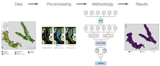
:Land cover and its change are crucial for many environmental applications. This study focuses on the land cover classification and change detection with multitemporal and multispectral Sentinel-2 satellite data. To address the challenging land cover change detection task, we rely on two different deep learning architectures and selected pre-processing steps. For example, we define an excluded class and deal with temporal water shoreline changes in the pre-processing. We employ a fully convolutional neural network (FCN), and we combine the FCN with long short-term memory (LSTM) networks. The FCN can only handle monotemporal input data, while the FCN combined with LSTM can use sequential information (multitemporal). Besides, we provided fixed and variable sequences as training sequences for the combined FCN and LSTM approach. The former refers to using six defined satellite images, while the latter consists of image sequences from an extended training pool of ten images. Further, we propose measures for the robustness concerning the selection of Sentinel-2 image data as evaluation metrics. We can distinguish between actual land cover changes and misclassifications of the deep learning approaches with these metrics. According to the provided metrics, both multitemporal LSTM approaches outperform the monotemporal FCN approach, about 3 to 5 percentage points (p.p.). The LSTM approach trained on the variable sequences detects 3 more land cover changes than the LSTM approach trained on the fixed sequences. Besides, applying our selected pre-processing improves the water classification and avoids reducing the dataset effectively by 17.6%. The presented LSTM approaches can be modified to provide applicability for a variable number of image sequences since we published the code of the deep learning models. The Sentinel-2 data and the ground truth are also freely available.
1. Introduction
Information about land cover and its changes are essential, for example, in natural resource management, urban planning, and natural hazard assessment and mitigation. Land cover classification and change detection are two crucial tasks in remote sensing, which have been addressed widely in the last few decades [1,2,3]. The two main reasons for this focus are the increasing availability of remote sensing data and the possibility of large-scale automatic land cover detection due to growing computing power and innovative machine learning (ML) approaches [4,5]. Additionally, modern multispectral satellites, such as the Sentinel-2 mission, provide data with high spatial and temporal resolutions [4].
The task of detecting land cover changes based on ML approaches with multispectral remote sensing data includes several challenges [6]. In the following, we briefly describe six of the main challenges. (1) The quality of the necessary land cover ground truth (GT) varies widely depending on the study region, the data source, available information about its creation, the spatial resolution, and the consistency of the class definitions [7]. (2) Besides the GT quality, the occurring classes vary from region to region. Therefore, individual case studies need to be conducted in the unknown region, enabling the ML approach to adapt to the local land cover characteristics. (3) Certain land cover classes differ mostly semantically. These semantic differences, for example, occur for urban classes, which include combinations of buildings with different purposes. (4) Concerning the temporal and spatial resolution of the satellite data, this resolution can be too coarse for some land cover classes. For example, the extent of buildings can be smaller than the size of one satellite pixel, which complicates the classification task of this specific class. (5) Another challenging task arises, for example, in the context of inland waters. During a year, the water levels can change, which results in a non-constant shoreline. (6) Our last considered challenge is about the validation of the land cover change detection. The distinction between land cover changes and possible misclassification requires appropriate measures to be defined and adapted concerning the specific study region [3,8].
In this study, we address these six challenges in the development and application of ML approaches on multispectral Sentinel-2 data. Our overall objective is to provide a methodological workflow, including deep learning approaches, that yields a robust land cover change detection addressing the six main challenges. Sentinel-2, as part of the Copernicus program, provides freely available multispectral data with adequate spectral and temporal resolutions for land cover change detection. The primary contributions linked to the study’s overall objective, as well as the novelties, can be summarized as follows:
- Novel Dataset: The majority of studies in remote sensing focuses on only a few available land cover datasets [9]. We present the first land cover change detection study based on a land cover dataset from the federal state of Saxony, Germany [10]. The dataset is characterized by a fine spatial resolution of 3 m to 15 m, a relatively recent creation date, and a representative status in its study region. Therefore, this dataset is highly valuable.
- Innovative Deep Learning Models: While there are successful artificial neural network approaches commonly applied in ML research, these approaches are often not popular in the field of remote sensing [11,12]. We modify and apply fully convolutional neural network (FCN) and long short-term memory (LSTM) network architectures for the particular case of land cover change detection from multitemporal satellite image data. The architectures are successfully applied in other fields of research, and we adapt the findings from these fields for our purpose.
- Innovative Pre-Processing: In remote sensing, there is a need for task-specific pre-processing approaches [5,13,14,15]. We present pre-processing methods to reduce the effect of imbalanced class distributions and varying water levels in inland waters to apply convolutional layers. Further, we discuss the quality and applicability of the applied pre-processing methods for the presented and future studies.
- Comprehensive Change Detection Discussion: No standard evaluation of ML approaches with sequential satellite image input data and a monotemporal GT exists. We present a comprehensive discussion of various statistical methods to evaluate the classification quality and the detected land cover changes.
In the following, Section 2, we commence by briefly presenting the related work in the context of land cover classification and land cover change detection. Subsequently, we introduce the used land cover dataset and satellite data in Section 3.1. In Section 3.2, the ML methodology is described before we present the results of our study in Section 4. The achieved results are discussed in detail in Section 5. Finally, we provide concluding remarks and an outlook for possible future studies in Section 6.
2. Related Work
The classification of land cover based on multispectral remote sensing data is, in current research, mostly based on supervised ML approaches. If remote sensing images are classified pixel-by-pixel, it can be referred to as image segmentation. The ML approaches can be categorized according to their input data: Pixel-based approaches, spatial approaches, and sequence approaches. The traditional pixel-based approaches classify each pixel individually based on the corresponding spectral data. Typical examples for pixel-based ML models in the classification of land cover from multispectral data are Random Forest [17,18], support vector machines [19], and self-organizing maps [6,9]. The main disadvantage of pixel-based approaches is that they ignore spatial patterns, including information about the underlying classification task. This disadvantage is relevant in land cover classification since land cover classes, such as farmland or water bodies, often cover coherent areas that are larger than one pixel. These correlations between neighboring pixels can not be used directly with pixel-based ML approaches.
Spatial classification approaches not only use one pixel for the classification but also use the two-dimensional (2D) spatial neighborhood. A popular spatial approach is based on 2D convolutional neural networks (CNNs) [20,21]. These CNNs consist of filter layers that can learn hierarchically: low-level features are learned in the first layers, more high-level features in the last layers. Most CNN approaches can only be applied monotemporally, meaning on one satellite image. Monotemporal land cover classification is difficult for classes, such as farmland and some forest classes, since their spectral properties change significantly over one year.
Sequence classification approaches are alternative approaches that are able to learn from a sequence of images. Deep learning examples for sequence approaches are recurrent neural networks (RNN), LSTM networks, and 3D CNN. The RNN and LSTM approaches are often combined with other approaches, such as 2D CNNs. The combination of CNNs and RNNs in the classification of land cover outperformed the studied pixel-based approaches in severall studies [22,23,24]. Qiu et al. [25,26] combine a residual convolutional neural network (ResNet) and an RNN for urban land cover classification. LSTM approaches, an extension of RNNs, are also applied in land cover classification [12,27], crop type classification [11,28], and crop area estimation [29]. Rußwurm and Körner [11] rely on an LSTM network with Sentinel-2 data and a GT, including a large number of crop classes. The proposed LSTM classifies some crop types inconsistently over two growing seasons. Besides, the study’s results imply that the LSTM approach can handle input data with cloud cover, and, therefore, no atmospheric corrections need to be applied. The LSTM application of van Duynhoven and Dragićević [27] demonstrates good classification performance even with few available satellite images. The LSTM approach of Ren et al. [28] achieves about 90% overall accuracy in a seed maize identification with Sentinel-2 and GaoFen-1 data. The LSTM network outperforms approaches, such as Random Forest.
Hua et al. [30] and You et al. [31] combine LSTM networks with 2D CNN and deep Gaussian processes. Besides, 2D CNNs can be extended from their 2D spatial convolution to 3D CNNs with an additional spectral axis for the convolution [32,33]. Another architecture for detecting changes in images are Siamese neural networks, which are applied on optical and radar data by Liu et al. [34], Daudt et al. [35]. Recent approaches, such as self-attention, are becoming more and more relevant in the field of multispectral remote sensing [30,36].
The detection of land cover changes can be divided into spectral-based approaches and post-classification approaches. Spectral-based approaches analyze the difference between the spectra from two or more multispectral satellite images to detect changes [1,2,37,38]. In contrast, post-classification approaches classify satellite images separately and compare the classification results afterward to detect changes [3,8]. The presented study relies on a post-classification approach to detect land cover changes.
3. Materials and Methods
In this section, we introduce the applied dataset and methods. We describe the dataset in Section 3.1 and the ML approaches for the land cover classification and change detection in Section 3.2. In Section 3.3, the evaluation methodology is explained in detail.
3.1. Dataset
For the presented land cover study, we use a land cover dataset consisting of GT and Sentinel-2 input data. We introduce the GT in Section 3.1.1, describe the Sentinel-2 data in Section 3.1.2, and explain our pre-processing in Section 3.1.3.
3.1.1. Land Cover Ground Truth
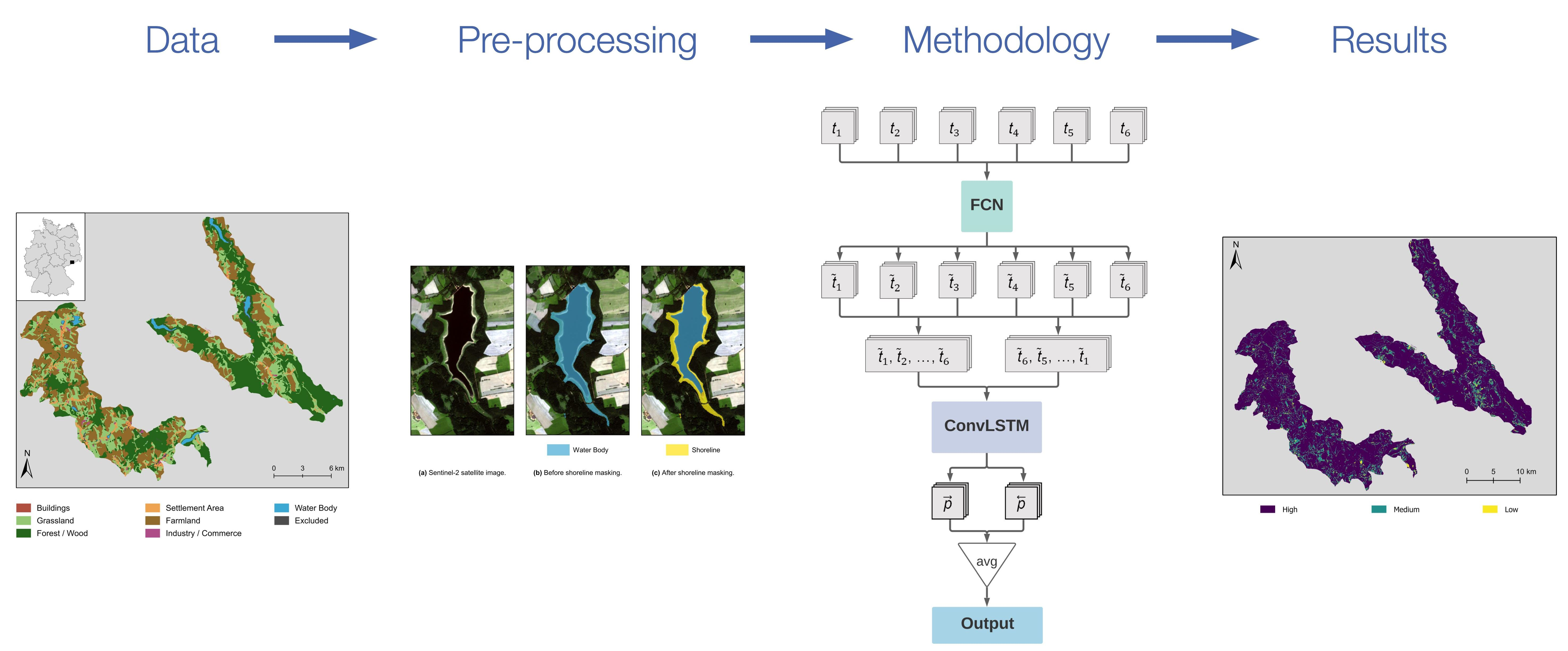
As GT, we rely on land cover vector data from the region around Klingenberg in the federal state of Saxony, Germany [10]. Klingenberg is located in the district Saxon Switzerland-Eastern Ore Mountains in about 500 above sea level and is a rural area in a low mountain range. This GT data covers an area of 234 2 with a spatial resolution of 3 m to 15 m. Figure 1 illustrates the GT aggregated in 2016 [10]. The GT consists of two separated parts. We have manually selected these parts to obtain one area of interest (AOI), including various features, for example, dams.
The land cover data consists of 14 land cover classes. In the following, only the seven classes with the largest class areas are considered: Forest/Wood, Farmland, Grassland, Settlement Area, Water Body, Buildings, and Industry/Commerce. The class Settlement Area contains the areas inside a settlement, which are neither buildings nor industrial or commercial areas. The smallest seven classes are summed up as Excluded, including railway systems and tracks, gardening, allotment gardens, sports and leisure facilities, roads and traffic areas, wasteland, and areas without available cover or use. We present an overview of all considered classes and their spatial coverages in Table 1.
3.1.2. Sentinel-2 Input Data
As input data, we rely on data from the freely available Sentinel-2 satellite program by the Copernicus program [4]. The Sentinel-2 program delivers multispectral imagery with 13 spectral bands from the visible and near-infrared to short-wave infrared. The Sentinel-2 imagery covers the Earth’s surface every five days with spatial resolutions of 10 , 20 , and 60 depending on the spectral band [4]. The resolution for the presented classification is transformed into pixels with the edge length of 10 . Pixels from spectral bands with a resolution higher than 10 are divided into arrays of pixels with the appropriate resolution of 10 . We refer to this spatial resolution as Ground Sampling Distance (GSD). We rely on the top-of-atmosphere L1C processing level, which already includes some pre-processing: radiometric corrections and geometric corrections based on a digital elevation model are already applied. The pixel values of each band are standardized to a mean of zero and a standard deviation of one.
3.1.3. Pre-Processing
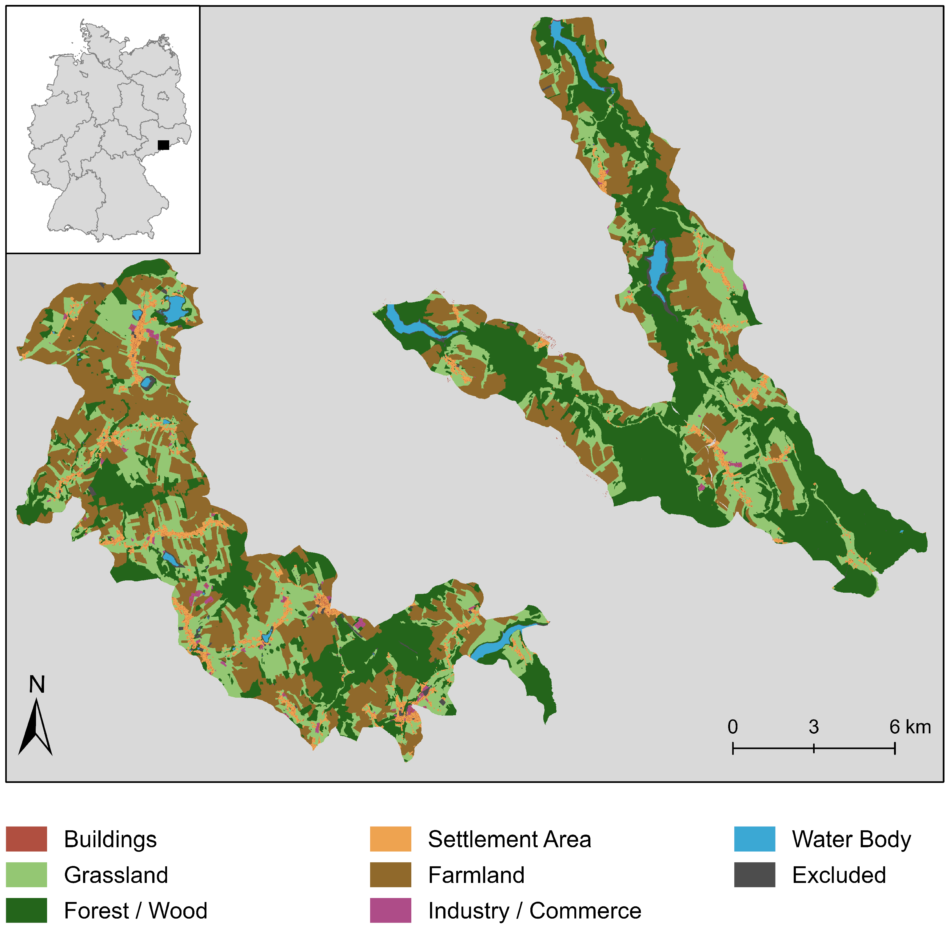
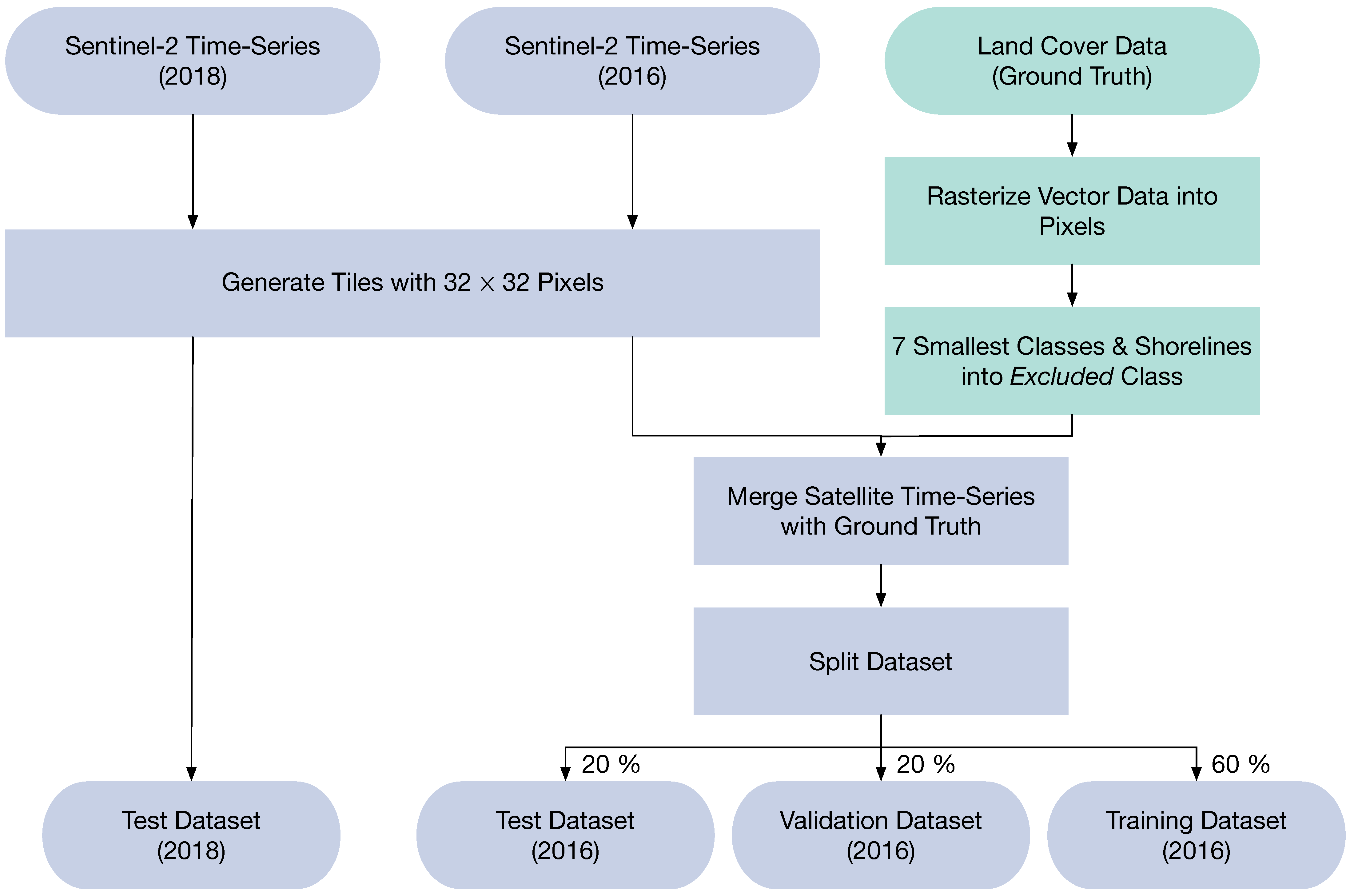
We apply pre-processing on the land cover dataset to prepare it for the land cover classification based on ML approaches. The pre-processing workflow for the dataset is shown in Figure 2. The GT is rasterized to a spatial resolution of 10 to match the Sentinel-2 imagery. In the next step, we sum up all pixels of the seven excluded classes into the class Excluded. The classes are reduced from 14 to 8 (7 plus Excluded) to balance out the classes. The intersection of the rasterized GT and the original vector GT areas per class is shown in Table 1. The intersection area is normalized with the area of the rasterized GT for each respective class. The percentage can, therefore, be interpreted as the portion of the rasterized GT that is overlapping with the correct class in the vector GT. In the ML classification presented in this study, the land cover data is split into tiles consisting of pixels. This tile size is motivated by the structure of the FCN model, which accepts multiples of 32 as tile edge lengths. The lowest possible tile edge length of 32 is chosen to provide a fair class distribution between the three subsets, even for small classes. Tiles are separated by a one pixel buffer. Only complete tiles can be used in the ML training. The introduction of the Excluded class, therefore, prevents tiles with excluded pixels to be removed from the dataset.
The AOI includes several water bodies with varying water levels, for example, water reservoirs. The area covered by water, therefore, also varies over time, as shown in Figure 3. For robust ML training, it is necessary to exclude the shoreline of these water bodies. To find the relevant shoreline pixels, we apply the Normalized Difference Water Index (NDWI) defined as
with B3 and B8 being the reflectance data of the third and eighth Sentinel-2 band, respectively [39]. B3 is characterized by a central wavelength of 560 and a bandwidth of 36 , B8 by a central wavelength of 833 and a bandwidth of 106 [4]. Pixels of the water body class with are interpreted as shoreline pixels and, therefore, added to the Excluded class. About 26.5% of the water body pixels are excluded.
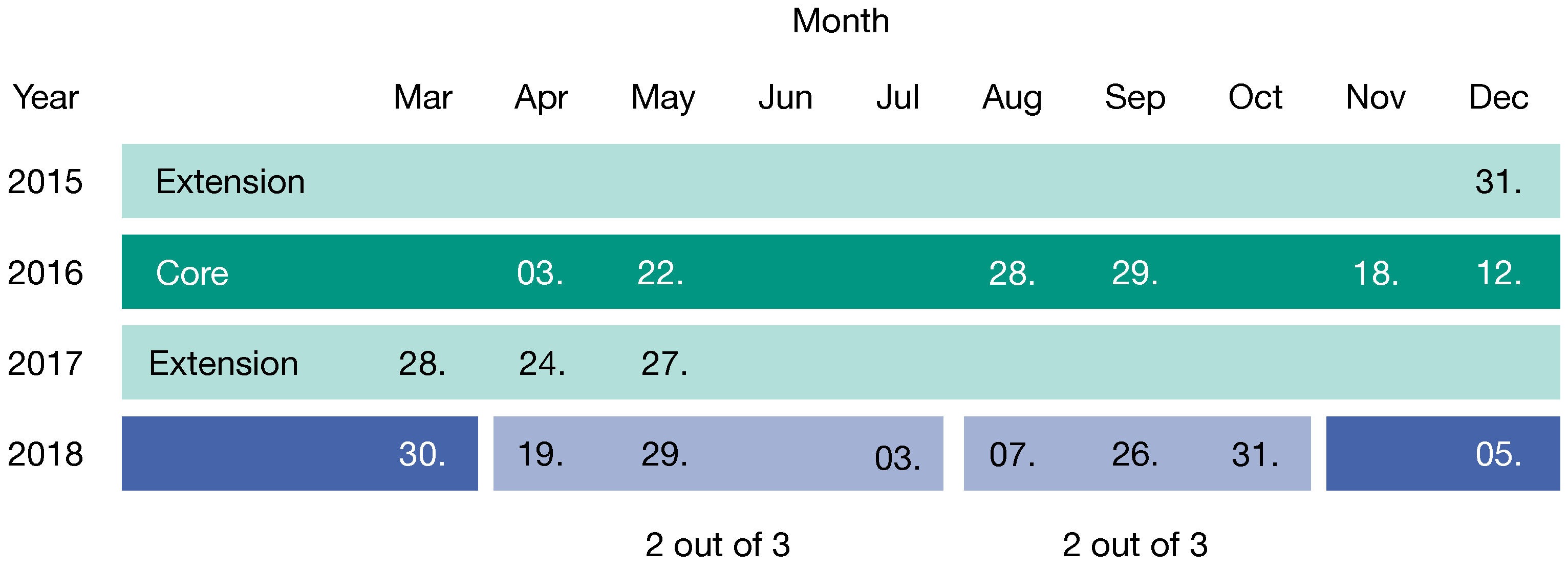
For the training of the ML approaches, the available Sentinel-2 satellite images of the year 2016 are used. Due to frequent cloud coverage in the region, images from the end of 2015 and the first half of 2017 are added to the training data, which increases the number of available images from six to ten satellite images. This procedure results in 1823 tiles per image, randomly split into training, validation, and test subsets with a 60%/20%/20% ratio. The randomization of the image tiles ensures an independent distribution of the subsets. With the split ratio, we follow standard ML guidelines [5,40]. For evaluating the land cover change and the transferability of the ML models, eight Sentinel-2 images from 2018 are used.
3.2. Deep Learning Methodology
As explained in Section 2, the task at hand can be categorized as semantic segmentation or pixel-by-pixel classification. We use two different model architectures of deep learning: in Section 3.2.1, we employ an FCN which uses monotemporal input data. A novel approach to using a sequence of satellite images and using sequential information with LSTM is presented in Section 3.2.2. Section 3.2.3 finally explains our usage of the data to train the FCN model and two approaches to train the LSTM model.
3.2.1. FCN Networks
This section gives a detailed description of the fully convolutional neural networks (FCN) model used. We also explain how we use a weighted loss function to treat pixels belonging to the Excluded GT class.
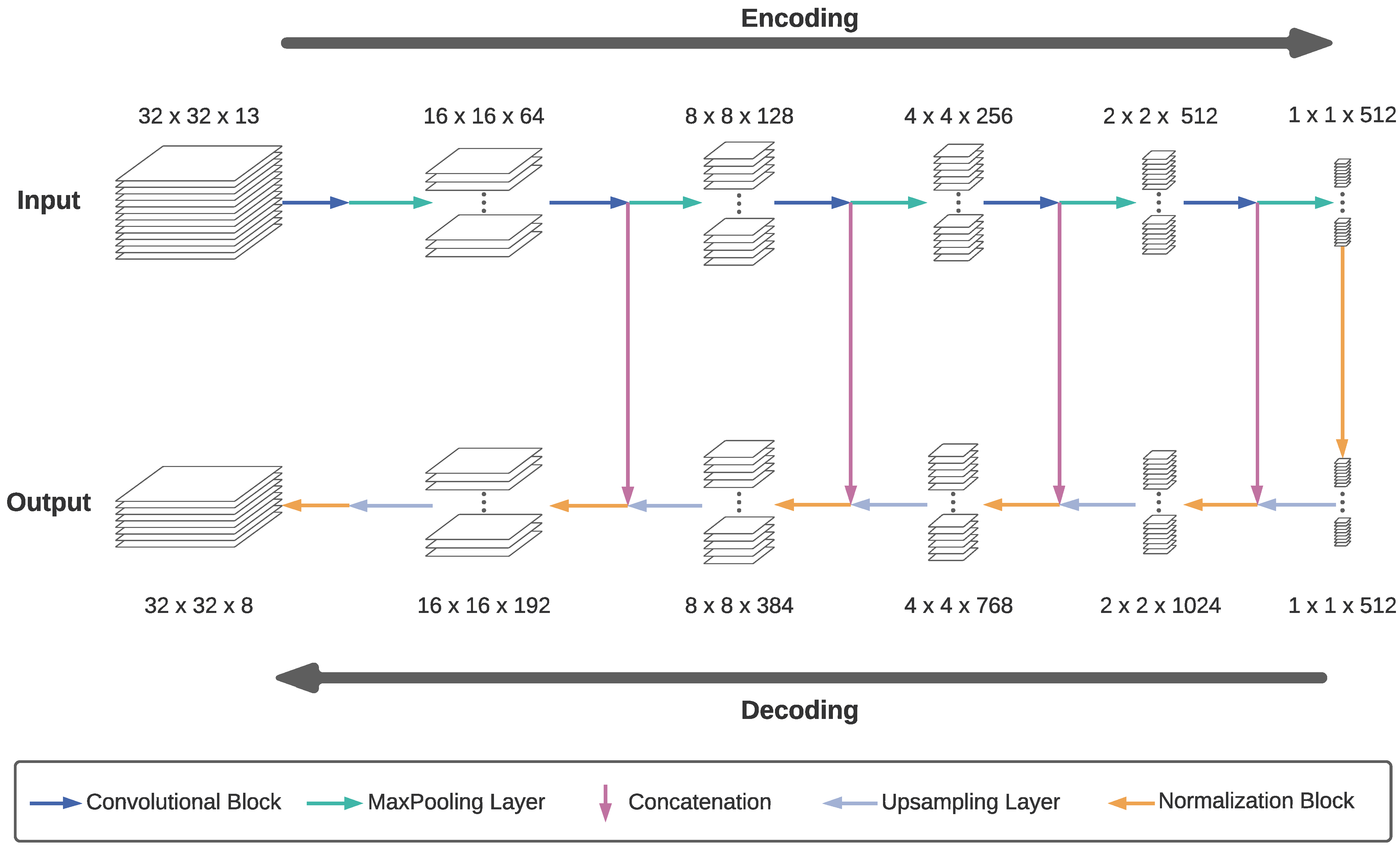
FCNs are successfully applied in semantic image segmentation [41], as described in Section 2. In this study, we apply an FCN with a modified U-Net architecture [42] that employs the image classification CNN VGG-19 [43] in its encoder stage. It is used to classify satellite image tiles of the dimensions into a classification output of the dimensions . Figure 4 shows the FCN structure in detail. Generally, the model consists of an encoder part, namely the VGG-19 without its final fully-connected layers, and a decoder part. While the image dimensions are reduced in the encoder stage, the global information of an image tile, meaning which classes are present in the tile, is extracted. The decoder stage scales up the image dimensions to their original extent. Skip connections between intermediate stages of the encoder and decoder part allow data to bypass the deeper stages of the encoder and decoder. These skip connections help to not entirely lose the local information of where a particular class occurs in the input tile, for example, the relative position in the tile. Without skip connections, the large number of five pooling and upsampling operations, respectively, would significantly impede the precision of the model. The combination of fully encoded and bypassed data with skip connections, therefore, can prevent this decrease of precision. The primary operations which are represented by arrows in Figure 4 are explained in detail as follows.
- Convolution block: Each of the five convolution blocks consists of several convolution layers; the first two blocks have two, and the last three blocks have four convolution layers. Each convolution layer has a kernel size and uses zero-padding to retain the input’s height and width. The number of filters is consistent in each block. From the first to the fifth block, the filter numbers are .
- MaxPooling: In general, a pooling layer has the purpose of reducing the size of its input. The so-called MaxPooling layer divides each image channel into -chunks and retains the maximum value of each chunk. Therefore, it reduces the height and width of the image by a factor of two.
- Concatenation: In this layer, the upsampled output of the previous decoder stage with the dimensions is concatenated with the output of the convolution block in the encoder stage that has the same height h and width w, but layers. The concatenated output has the dimensions .
- Upsampling layer: The upsampling layer doubles the height and width of an image by effectively replacing each pixel with a -block of pixels with the same value.
- Normalization block: The normalization block consists of two sub-blocks with a convolution layer followed by a batch-normalization layer and a Rectified Linear Unit (ReLu, ) activation layer each. While preserving the input image dimensions, the input activations are re-scaled to have a mean of zero and a standard deviation of one by the batch-normalization layer.
The dimensions of the input, output, and intermediate data shown in Figure 4 are given for our training tile dimensions of and eight output classes. Due to the reduction by a factor of 32 in the encoder stage, the 32 outermost pixels of an image are affected by the zero-padding with this model. With a tile size of in our case, all pixels are affected by the zero-padding. Due to the input standardization to a mean of zero, as mentioned in Section 3.1.2, this effect is minimized.
The output of the image segmentation model for each pixel in the tile is a vector with an entry for each of the eight classes. The softmax activation is then used to normalize that vector:
with the indices i and j denoting the i-th and j-th class. So, can be interpreted as the prediction probability of the pixel belonging to class i.
The training batch for the FCN is built by sampling 60% from all available tiles of the six dates available in 2016. The training of the FCN is performed monotemporally, meaning that the training data from different available dates are not stacked together but used separately. In that way, the FCN learns from satellite images of different seasons and phenological phases but without any sequence information, such as date and order of the images. This baseline FCN model is further referred to as and is used as a monotemporal baseline model. Once trained, it is also used as a pre-trained core model in the following FCN+LSTM model.
As loss function L for the training of the FCN, a weighted categorical cross-entropy is used, which is defined as:
Again, the index i refers to the class. is the softmax-transformed network prediction for class i and is the GT vector of the respective pixel. If the pixel belongs to class i, , all are of value zero. For the class weights vector , the inverse number of GT pixels are used for the seven classes of interest in order to stronger penalize misclassifications of infrequent classes. The class weight of the additional Excluded class is set to zero. Pixels belonging to this Excluded class do not contribute to the loss of a tile. We can use tiles in training that include Excluded pixels without a negative influence on the training. Both the FCN model and the loss function are adapted from Yakubovskiy [45].
3.2.2. LSTM Networks
This section introduces the concept of LSTM cells and shows how they are implemented in our combined approach with an FCN model. The complete schema of this combination is illustrated in Figure 5.
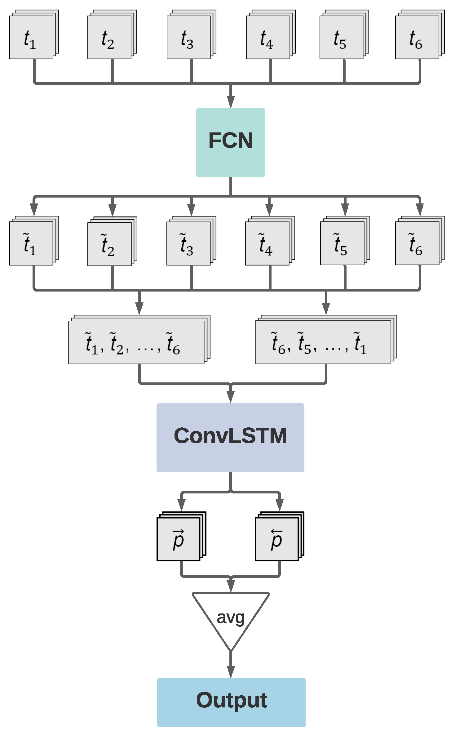
To fully benefit from the sequence information in the satellite images, we combine the presented FCN architecture with LSTM networks. An LSTM network is a type of RNN designed to resolve vanishing gradients with backpropagation through time. The output state of an LSTM cell after iteration t relies on the newest input and its previous output state and a so-called hidden state , which is used for internal computation. The calculation of the LSTM output is modulated by three gates: input, output, and forget gate. The forget gate determines to what extent the previous cell state is remembered. The input gate determines how strongly the new input contributes to the new cell state. Finally, the output gate is used to calculate the new hidden state . Our approach uses a 2D convolutional LSTM cell. The LSTM cell has, therefore, a kernel which is convolved over its input. The complete FCN+LSTM schema is shown in Figure 5.
Its input data has the dimensions of . In the case of the training dataset from 2016, satellite images of six dates are available. One sample, therefore, consists of the same tile at six different dates, to , brought into chronological order. Each tile of that sequence is processed individually by the FCN, , omitting the final softmax activation of the FCN. The six FCN outputs to are then stacked as a sequence both in chronological and reverse chronological order, referred to as bi-directional. This bi-directional architecture allows the LSTM to learn from previous and subsequent steps in the time sequence. The two intermediate output sequences of the dimensions are then passed into the convolutional LSTM cell, further referred to as ConvLSTM. Both the output of the forwards-directed and the backward-directed sequence, and , are transformed by a final softmax application and then merged as the final output via averaging.
3.2.3. Model Training
In this section, we give a complexity comparison between both presented models and explain the training procedure. With an extension of the imagery to late 2015 and early 2017, we present an alternative approach to training the LSTM model using a variable selection of image dates.
Table 2 shows the number of trainable parameters for the two models we employ, the FCN and FCN+LSTM, as well as a modified VGG-19 for comparison. The modification of the VGG-19 consists of accepting 13 input channels instead of the usual three of an image and having eight output classes. The comparison shows that going from image classification (VGG-19) to image segmentation (our FCN, based on VGG-19) increases the number of trainable parameters by about 45% (nine million). Using a ConvLSTM layer after the FCN, however, adds virtually no trainable parameters, namely 9280. The model complexity of the FCN+LSTM in terms of trainable parameters is, therefore, practically equal to the FCN. It has to be noted that although not many trainable parameters are added to the model, every step of the input sequence now passes the FCN instead of the monotemporal input before. In each full FCN+LSTM inference step, the FCN has to infer instead of one, which slows down the individual training steps.
Training sequences for the FCN+LSTM model are built in two different ways: A fixed sequence and a variable sequence approach. In the fixed sequence approach, the six images available for 2016 are exclusively used to build the training sequence. In the variable sequence approach, however, the sequential input data is built from the extended training pool of ten images described in Section 3.1. Thus, for each training batch, six out of the ten available images are randomly sampled and put into chronological order. The desired amount of image tiles is then again sampled from all available tiles to achieve the desired batch size. Figure 6 illustrates the specific dates of the available satellite images. The FCN+LSTM model trained with the fixed sequence is referred to as , and the FCN+LSTM trained with the variable sequence as . FCN+LSTM will also be shortened to LSTM since the LSTM cell distinguishes the model from the monotemporal FCN model.
Image augmentation based on horizontal and vertical image flipping and rotations is applied in the training to artificially enrich the training dataset and to prevent overfitting. Each of the three models (, and ) is trained five times. Every time, the model weights are randomly initialized anew. Ensembles are formed using some or all of the five models by averaging the individual class probabilities before selecting the most probable class. The best ensemble is selected for each approach by its overall accuracy.
3.3. Evaluation Methodology
In this section, we present the methods used to evaluate all trained models. We use Sentinel-2 imagery from two years, 2016 and 2018, for the evaluation. Section 3.3.1 addresses the evaluation with the test subset of the imagery from 2016. In Section 3.3.2, we use the more recent imagery of 2018 to evaluate the predictions of the LSTM approaches on new image sequences.
3.3.1. Evaluation Metrics for the 2016 Classification
Since the GT originates from 2016, the classifications performed on the Sentinel-2 images from 2016 are used to calculate accuracy metrics. In this section, we introduce the relevant metrics and explain the evaluation procedure for the monotemporal , as well as the multitemporal and the .
As shown in Figure 6, six satellite images are available for 2016. Since the and the use a six-image sequence, but the operates on single images without sequence information, we need to consider two cases. Case 1 concerns the classification with the . The classifies each image tile individually for every one of the six images. Each classification result is compared with the respective GT tile. Subsequently, the evaluation metrics are averaged over the tiles of all six dates. Case 2 counts for both LSTM approaches. To evaluate both LSTM approaches, we build a six-image sequence for each test tile and classify these sequences. The result is compared with the respective GT tiles.
For the evaluation of the land cover classification, we rely on several metrics. The prediction for a pixel with regards to the GT can be one of four types: true positive (tp), true negative (tn), false positive (fp), and false negative (fn). True and false correspond to the equality of the prediction with the GT, while positive and negative correspond to the class for which the metric is calculated. Overall accuracy (OA), precision, and average accuracy (AA) are defined as
Each metric is calculated class-wise as for every class c, then the unweighted average is calculated as:
with the normalization factor for the seven classes considered. We do not calculate the metrics for the Excluded class.
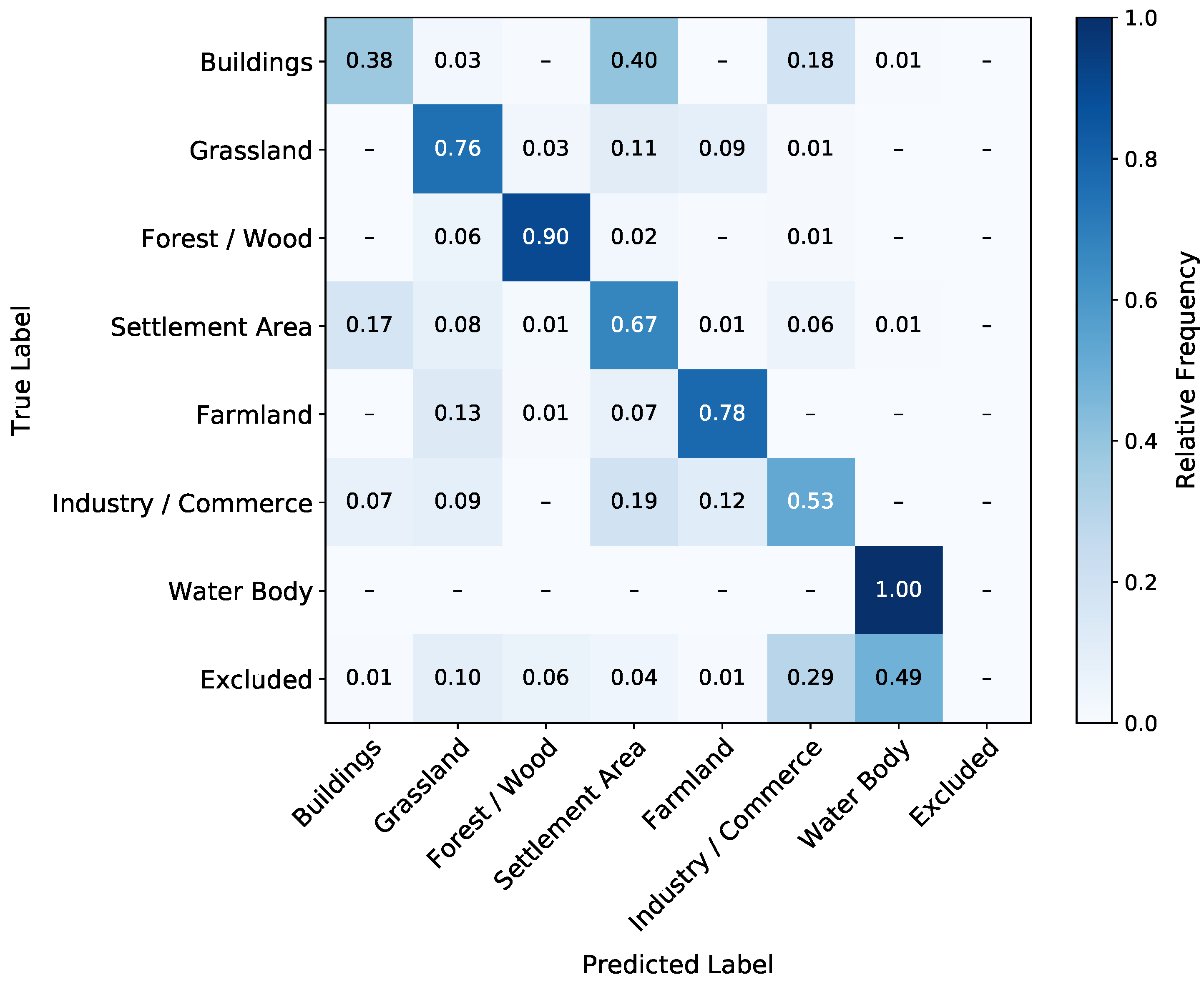
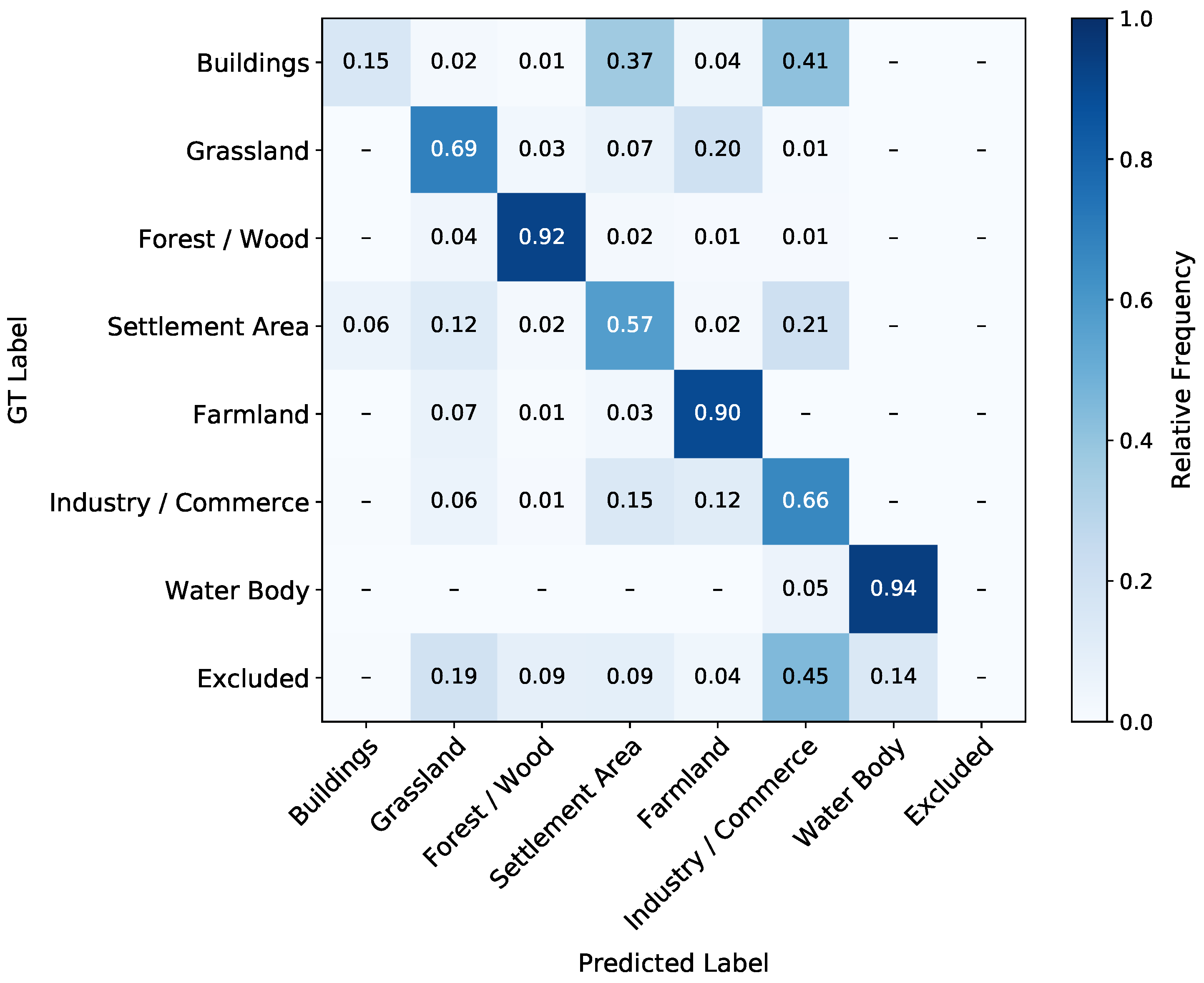
In general, confusion matrices are a visualization of precision and AA. In confusion matrices, the true labels are shown over the predicted labels. The AA is the average of the class-wise accuracies, which are the diagonal elements of the confusion matrix. The precision is the average of the class-wise accuracies normalized by the sum of the class-wise number of predicted labels (vertical axis).
With the probabilities for each class in the observed data, Cohen’s Kappa is defined as
3.3.2. Evaluation Metrics for the 2018 Classification
In this section, we introduce a robustness evaluation concerning the image selection using the LSTM approaches’ predictions on multiple sequences of 2018 satellite images. We, therefore, propose a voting scheme for the predictions on multiple image sequences.
We train the with variably built sequences out of a pool of ten images. In contrast, the is trained on the six dates in 2016 that also form the test subset. Therefore, the naturally might perform worse on this test subset since the is not trained on these exact six dates. This aspect is reasonable as Sentinel-2 satellite data can be unavailable for the most similar and prospective dates due to, for example, cloud coverage. Therefore, robustness against different temporal spacing in the image sequence compared to the training data is crucial in evaluating a model.
We evaluate whether an LSTM trained on a fixed time sequence of satellite images has similar predictions upon using different time sequences. To address this evaluation, we use six sequences with six out of eight satellite images in 2018, as shown in Figure 6. Both LSTM approaches predict based on these six sequences. The resulting six classifications maps are evaluated regarding their similarity to both the GT and each other. Inter-similarity between the six classification maps is evaluated in the form of a voting scheme with the following three categories:
- Unison vote: A pixel is classified in unison.
- Absolute majority: The same class is assigned to a pixel in four or five classification maps.
- No majority: There is no class that is assigned to a pixel in four or more classification maps.
We interpret the inter-similarity of classifications with different input time sequences in a year to measure confidence in the prediction. For example, a confident classification by unison or absolute majority of a coherent patch of pixels might hint to an actual change of the GT from 2016 to 2018. Further on, classifications made by unison vote are denoted to be of high confidence. Classifications made by an absolute majority are denoted as medium confidence, and lastly, classifications made with no majority are denoted as low confidence. For the final classification map of the AOI, pixels classified in unison or by absolute majority receive the majority vote’s class label. For pixels without a successful majority vote, the class probabilities are summed over the six sequences, and the class with the highest cumulated probability is chosen.
4. Results
In the following, we present the classification results. Section 4.1 focuses on the evaluation with the satellite images of 2016 as test data. The GT is considered up-to-date for this year. Section 4.2 presents the results for the robustness evaluation of the LSTM models against different image sequences from 2018.
4.1. Classification Results with 2016 Satellite Data
Table 3 presents the prediction scores on the test subset of the 2016 satellite data compared to the GT. For the , the ensemble with the highest overall accuracy score combines all five trained models. Both LSTM models use three individual models in their best-scoring ensembles. Overall, the best ensembles show about 1 to 3 percentage points (p.p.) better results per evaluation metric. The standard deviations of the OA across five training runs range from 0.3–0.8%. The five models of each model category , , and show relatively similar results.
In the following, we focus on the results of the respective best ensembles. The best OA (see Equation (4)) is produced by the with 87.0%, followed by the with an OA of 84.8%. The achieves an OA of 81.8%.
The precision and AA results are defined in and visualized in Equations (5) and (6) and visualized in the confusion matrices in Figure 7, Figure 8 and Figure 9. The values for the precision are not weighted per class size, as described in Section 4.1. The precision, with values from 60.1–64.2% for the three best ensembles and the AA (71.6–73.2%) are significantly lower than the OA. Similarly to the OA, the precision increases about 3 from the to the . In contrast, both LSTM approaches achieve nearly the same precision of about 62.6–64.2%. In terms of the AA, the performs best with 74.7%, followed by the with 73.2%, and the with 71.6%.
Cohen’s Kappa (see Equation (8)) results in 74.8–82.0%. Adding sequential information leads to an increase in of 4.3 to 7.2 , which is larger than the increase in OA.
With the normalized confusion matrices for all three models in Figure 7, Figure 8 and Figure 9, we subsequently focus on the accuracies for each class. All three models achieve 100% accuracy for Water Body. Next in accuracy follows the Forest/Wood class with 90–93%, then Farmland with 78–88% and Grassland with 76–81%. Adding sequential information increases the classification quality in these classes. Further, Buildings, Settlement Area, and Industry and Commerce, are significantly confused by all three models. Compared to the , the classification quality of the slightly decreases in Buildings, Settlement Area, and Industry/Commerce. The class with the lowest accuracy for all three models is Buildings. Pixels of this class are predicted into the Settlement Area class at least as often as they are correctly predicted. Here, all three models score 37–38%, with the ’s score being the highest. Regarding the two LSTM approaches, the achieves higher scores for the classes Forest/Wood, Farmland, and Grassland. Consequently, the has higher scores for Settlement Area, Industry/Commerce, and Buildings.
4.2. Classification Results with 2018 Satellite Data
Table 4 presents the confidence statistics for the and , according to the confidence definition in Section 3.3.2. The shows with 88.3% unison votes an about 3 larger amount of pixels with high confidence than the . The number of pixels in agreement with the GT is a subset of the total number of pixels regarding voting. With 76.9%, the classification is in better agreement with the GT than the with 75.4%. With the variable satellite image sequence as training data, the predicts more land cover change with high confidence. Upon considering all confidence levels equally, both LSTM approaches predict virtually the same ratio of changed pixels (17.0% and 17.1%).
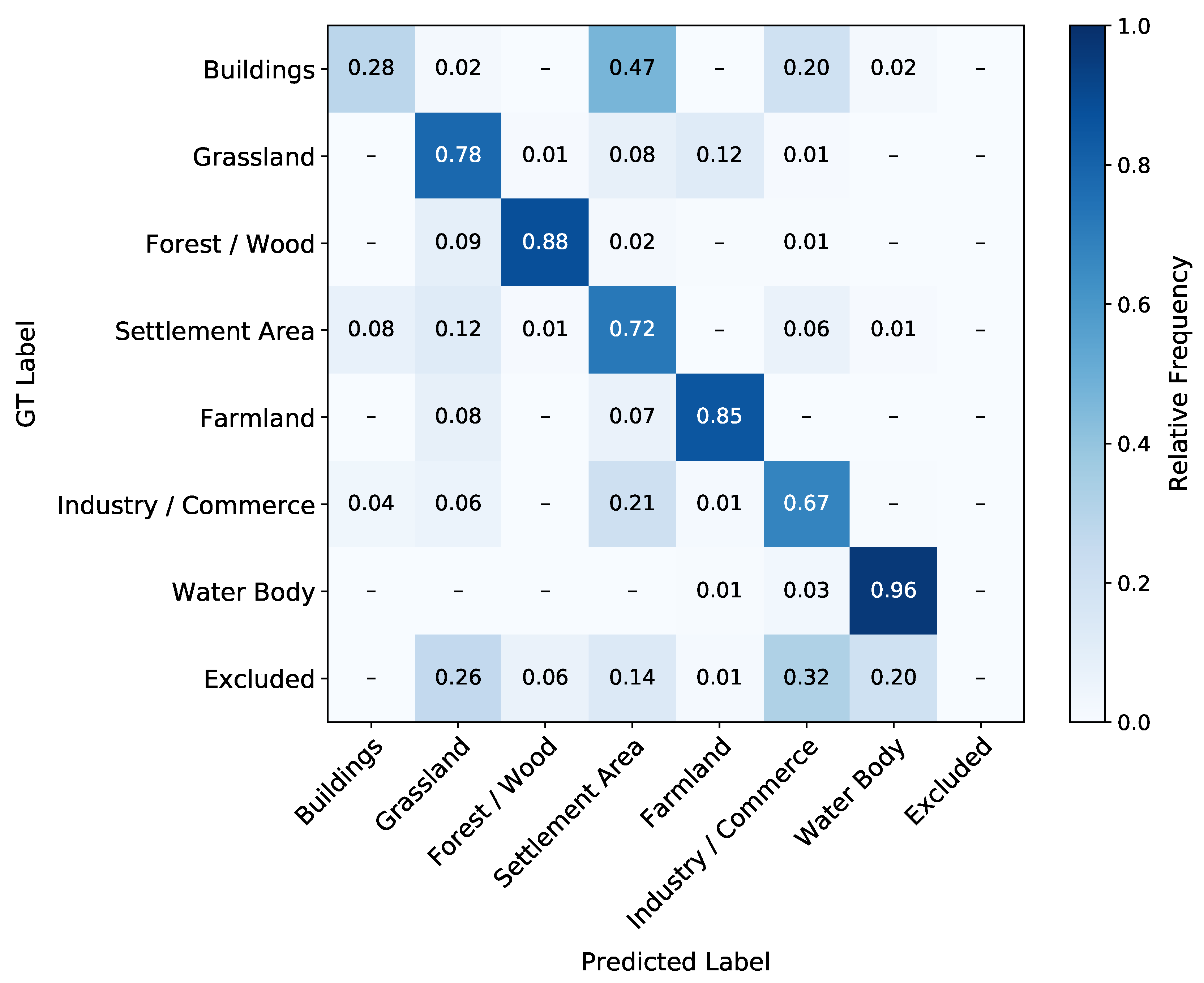
Similar to the 2016 test subset prediction in Section 4.1, we create the confusion matrix between the GT class labels and the LSTM predictions ( or ). The confusion matrix of the () for the 2018 classification is shown in Figure 10 (Figure A1). We compare this matrix with the confusion matrix of the 2016 classification in Figure 8. It is important to note that the confusion found in the 2018 classification can result from similar reasons as in the 2016 classification and, additionally, can result from land cover changes between the years 2016 and 2018. Two main changes are noteworthy. Firstly, the class Buildings is significantly more confused with Settlement and Industry/Commerce than in the 2016 classification (see Section 5.1). The second main change is that Grassland is confused more frequently with Farmland.
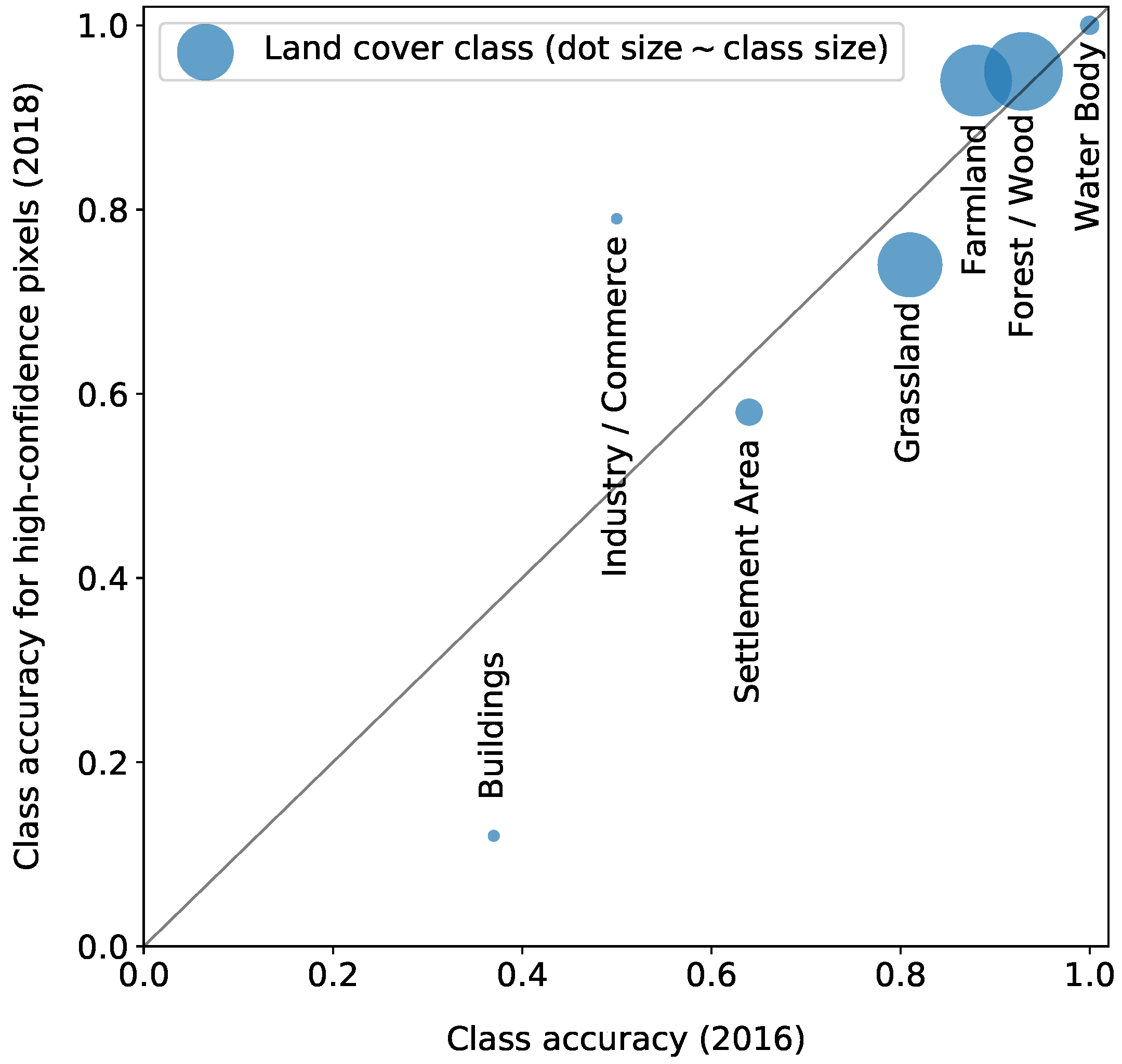
Subsequently, we compare the per-class percentages of predictions in agreement with the GT against the per-class accuracy of the 2016 predictions. Figure 11 illustrates the resulting calibration plot for the predictions in 2016 and 2018. The class sizes are also included to show possible fluctuation effects for smaller class sizes.
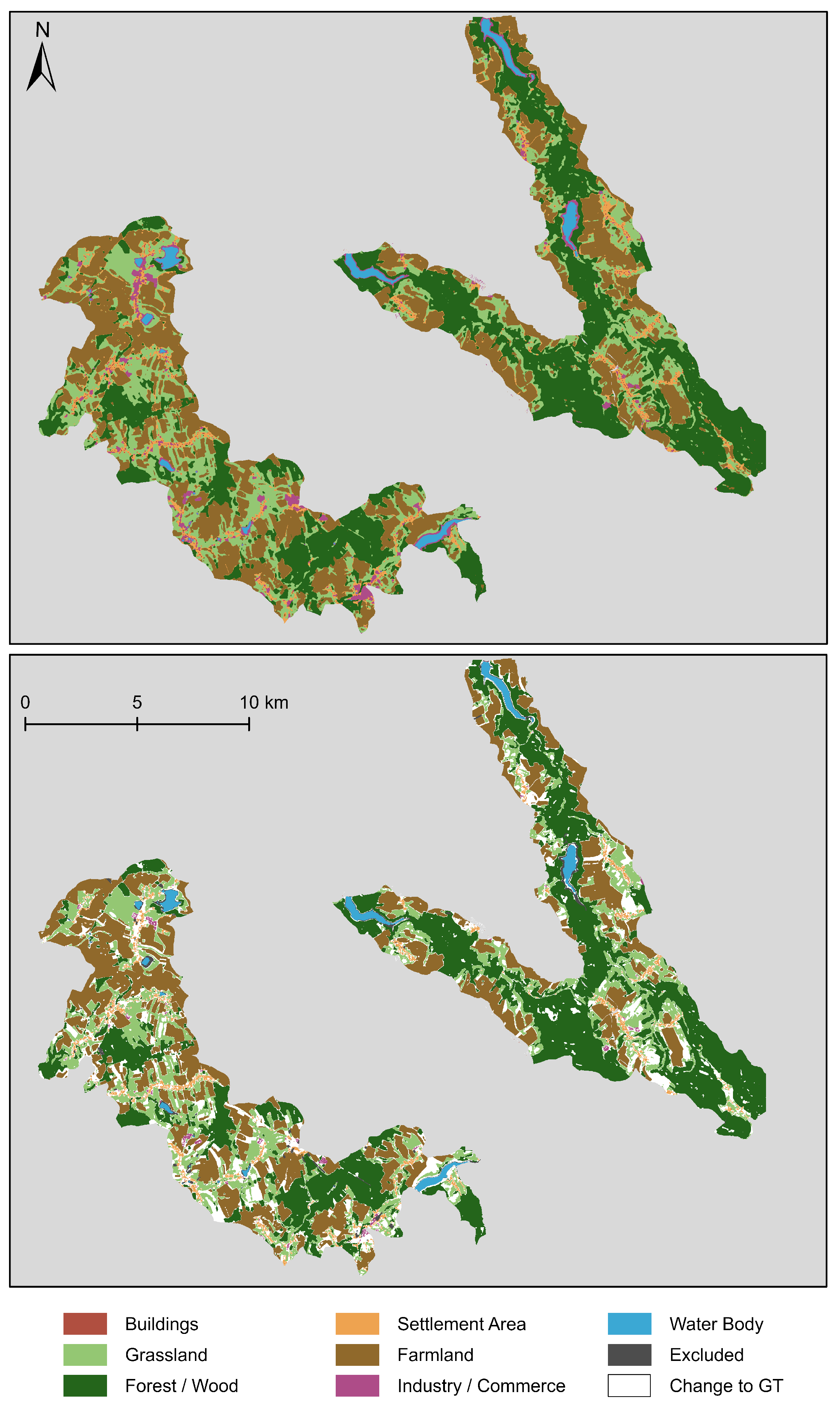
Figure 12 illustrates the 2018 classification of the and the differences between this classification and the GT. Overall, the classification map is smooth with large coherent areas. Most of the changed pixels compared to the GT can also be found in coherent areas. The most considerable changes occur primarily in regions with Farmland land cover and areas near the class Forest/Wood.
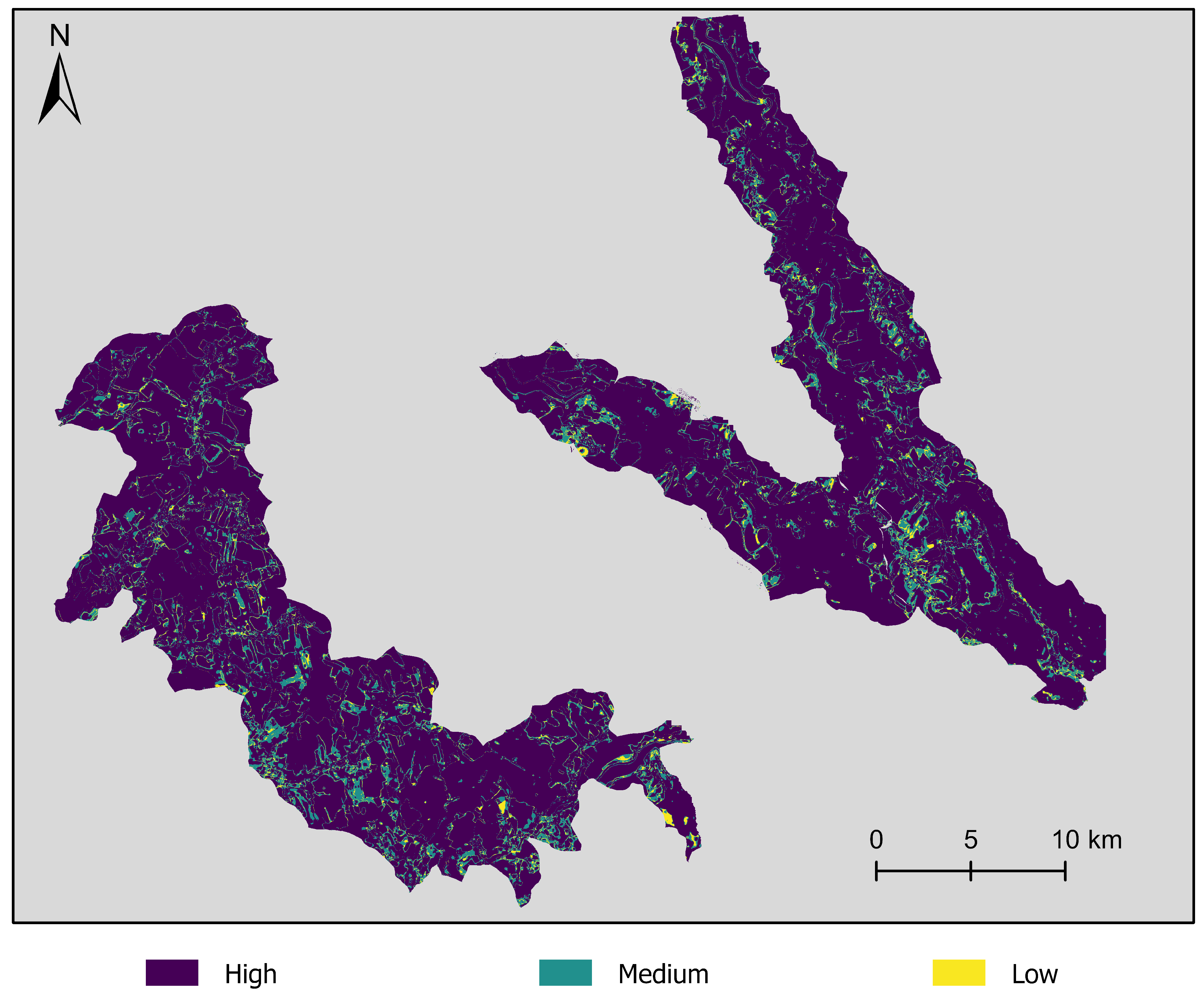
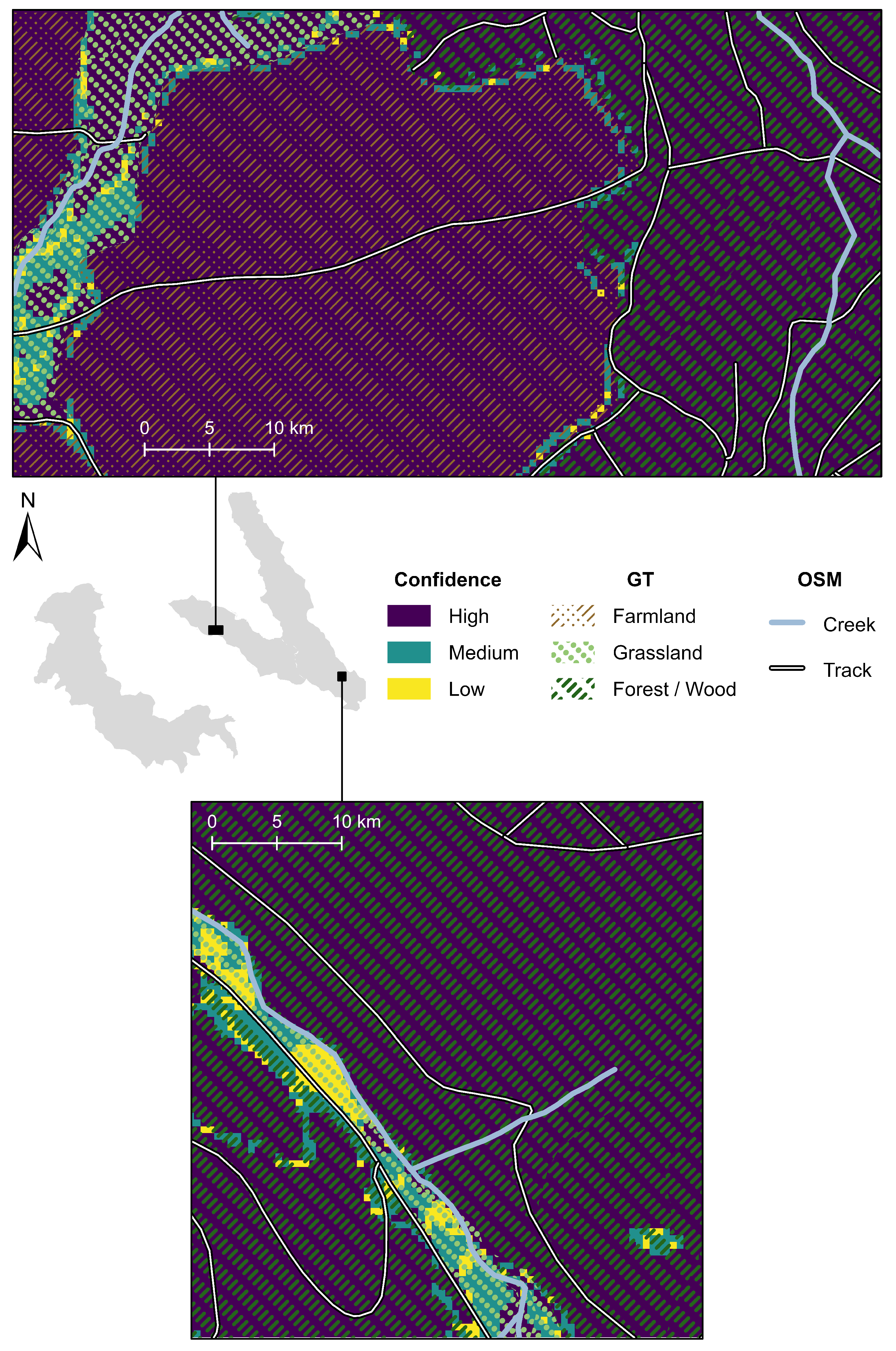
Figure 13 visualizes the distribution of the three confidence levels over the AOI. Besides, Figure 14 presents an enlarged detail of the AOI regarding two specific regions and their confidence levels. Both enlarged details show the confidence level, the given GT land cover class, and additional information, such as creek and track, extracted from OpenStreetMap (OSM). Based on these details, we can evaluate a possible correlation between class borders and low-confidence prediction. Large parts of these example areas are classified with high confidence. In the upper part of Figure 14, the pixels with low and medium confidence are distributed around GT class borders of the classes of Farmland, Grassland, and Forest/Wood.
5. Discussion
In this section, we discuss the results of Section 4. In Section 5.1, we discuss the quality of the 2016 classification results in detail. In Section 5.2, the 2018 class accuracy of high-confidence pixels is evaluated based on the 2016 class accuracy. Subsequently, we present a comprehensive discussion of the detected land cover changes in Section 5.3. The applied pre-processing is evaluated regarding the shoreline masking and the class exclusion in Section 5.4.
5.1. Classification Quality
To evaluate the classification quality of the presented models, we refer to the classification results based on the 2016 data in Section 4.1. Regarding the stability of training, all three models show low standard deviations of 0.3–0.8% for the OA across five training runs each. That means that the training of these models is robust against the selection of their random seeds.
As presented in Section 4.1, the highest OA is produced by the . This finding implies that by training on a fixed satellite image sequence, the model ensembles can better adapt to the dataset. Furthermore, since the fixed satellite image consists of data from one year (2016) rather than from several years as the variable sequence (2015–2017), the training can be more meaningful. Including satellite images of the previous year, 2015, or the following year, 2017, does not add measurable value to the training, as the smaller OA for the shows. The overall good result of the is surprising since it does not train based on sequential information, meaning the satellite images’ temporal order. However, we can note that the sequential information increases the OA about 3 to 5 and adds value. The much lower AA and precision results compared to the OA can be explained by the class imbalance of the dataset. The AA results imply that training on a variable satellite image sequence is more beneficial for the smaller classes in the dataset.
In the following, we discuss the comparison of the individual class accuracies between the and (see Figure 7 and Figure 8). We can note that the classes Forest/Wood, Farmland, and Grassland can be classified significantly better with the sequential information used by the LSTM approaches. In general, these three classes are expected to show a significant variation over a year due to phenological phases that include harvests in the case of Grassland and Farmland. The confusion of the three classes with the lowest accuracy scores, Buildings, Settlement Area, and Industry/Commerce, can be explained by their composition: they can include grassland and buildings that can not be differentiated from Industry/Commerce. These three classes are not expected to show much change over the curse of one year. Regarding the strong confusion of Buildings with Settlement Area, it appears plausible that the GSD of 10 (see Section 3.1.2) is a substantial limiting factor for that classification. Individual buildings cannot be resolved well with the given GSD, which leads to buildings sometimes being represented by a single pixel in the rasterized GT. The resulting slight decreases in classification quality can be due to changes in the respective land cover or fluctuations.
The confusion of Buildings and Settlement Area can also be partly explained by the intersection area in Table 1. We can see that only 65.7% of the rasterized Buildings class intersects with the Buildings class in the vector GT. This is the least intersection percentage by a margin of 18%. Twenty-eight and four-tenths percent of the Buildings class in the rasterized GT actually intersect with the Settlement Area class in the vector GT. Essentially, the Buildings class is already considerably confused with Settlement Area in the rasterized GT due to the large pixel edge length compared to many building polygons.
The ’s lower class accuracies for the phenologically changing classes Forest/Wood and Farmland compared to the show the benefit of the fixed sequence training for these classes. However, the higher accuracies for the lowest three classes implies that the variable sequence () improves the classifier’s robustness for classes that are, in general, more difficult to learn.
The lower values for Cohen’s Kappa compared to the OA are expected, since removes by-chance agreements from the classification results. The large increases of for both LSTM approaches compared to the FCN again show the benefit of processing sequential information.
Since we present the first land cover classification and change detection study on this GT in Klingenberg, Germany, no other published results are available for a direct comparison. To put our results in perspective, we discuss the results of Rußwurm and Körner [12], Ren et al. [28] in the following. The sequential recurrent encoders approach of Rußwurm and Körner [12] achieves an overall accuracy of 90% on 17 crop type classes. This result is similar to our presented LSTM results on the Farmland and Forest/Wood class. The size of the training dataset is more than 18 times larger than the presented dataset, which implies that our approach will benefit from an increased training dataset. In Ren et al. [28], the presented LSTM approach achieves 90% in a pixel-based classification with three classes. The LSTM only slightly outperforms approaches, such as Random Forest and support vector machines, which implies that the value of using sequential data is marginal in this dataset. For our presented and the two compared studies [12,28], it would be interesting to evaluate the exact quality of the GT to estimate the maximum achievable overall accuracy.
5.2. Accuracy Evaluation
As stated in Section 3.1.1, the GT is accurate for the year 2016. Using the GT to evaluate the 2018 classification can lower the accuracy measures since, in addition to misclassifications already found in 2016 (see Section 5.1), land cover changes can decrease the accuracy metrics. In this section, we compare the 2016 class accuracy of all pixels with the 2018 class accuracy of high-confidence pixels in order (a) to evaluate if the applied confidence measure is adequate and (b) to find first implications of land cover changes.
Figure 11 shows the accuracy per class of high-confidence pixels for the 2018 classification over the individual class accuracy of the 2016 classification for the . Overall, the accuracy per class of the high-confidence pixels in 2018 is similar to the percentage of correctly classified pixels in 2016. This finding implies that the approach we use to calculate and apply the confidence measure based on the voting of six predictions is adequate.
The two largest classes (see Table 1), Forest/Wood and Farmland, and the Water Body class, show good accordance between the class accuracy measures. This result implies that these classes are not prone to significant land cover change between 2016 and 2018. The third-largest and fourth-largest classes Grassland and Settlement Area are characterized by a significant difference between both accuracy measures. For both, the 2018 class accuracy is lower. This finding implies land cover changes in this class.
Concerning the two smallest classes, the urban classes Buildings and Industry/Commerce, the accuracy measures of 2016 and 2018 differ vastly. While these differences can imply land cover changes, they can also originate from (a) statistical fluctuations due to the small class sizes or (b) from confusion with the respective other urban class. In the following, Section 5.3, these results are further discussed. Note that the confidence measure is used without any form of calibration.
5.3. Change Detection
In this section, we discuss the change detection between 2016 and 2018 for the and the . Note that if the classification results of both LSTM approaches are similar, we exemplarily regard the results of the approach.
We find two main changes between the confusion matrices of 2016 and 2018 in Section 4.2. The more significant confusion of the urban classes is expected since these classes’ differences are often semantic, and changes within these classes, such as new buildings, are quite frequent in Germany. The confusion of Grassland with Farmland is expected since both classes have a high variability over a year, and farmland can be transformed into Grassland. We can derive similar results from the confusion matrix of the in Figure A1. The accuracy evaluation in Section 5.2 comes to a similar conclusion about possible land cover changes and confusion. The most considerable changes visualized in Figure 12 are in regions with Farmland land cover and areas near the class Forest/Wood. These changes are expected since those are the classes that change most during a year. Rußwurm and Körner [11] explain similar confusions by seasonally-variable conditions of the environment.
The findings from Figure 14 have multiple implications: (a) the GT classes are not well defined at the border, (b) the class borders are floating, meaning that, for example, there is no clear border between Grassland and Forest/Wood, and (c) there are other effects, such as shadows from trees and other plants, at the class borders. In the lower example area of Figure 14, the pixels with low and medium confidence are clustered around one particular track parallel to a creek. This finding implies that (a) the land cover around this track and creek can be ill-defined, (b) the land cover can change due to construction work, and (c) other effects, such as flooding, can play a role here.
One assumption of the presented study is that a closed set of land cover classes is known before training the deep learning models. Another approach is called open-set classification [46,47], where unknown or novel classes are included in the dataset. The models then are not only applied for change detection but also for the exploration of new land cover classes. In the presented study, the assumption of a closed set of land cover classes is adequate due to two reasons: (a) because we compare satellite images with only two years difference, and (b) because the probability of novel or unknown classes in this small region in Germany is small.
5.4. Evaluation of the Pre-Processing
In this section, we analyze and discuss the effects of the two pre-processing steps Shoreline Masking and Class Exclusion. The exclusion of pixels from the Water Body class is due to the visual discrepancy between water bodies in the GT and the satellite images (see Figure 3). Especially when working with satellite images from different dates and seasons, varying water-level can be expected, and a constant GT can not cope with this difference. As shown in Figure 3, the NDWI-based exclusion approach presented in Section 3.1.3 distinguishes well between actual water and shoreline pixels upon visual examination. Since we have only trained models using the GT with applied shoreline masking, a before-after comparison is impossible. As seen in Figure 7, Figure 8 and Figure 9, however, all three models manage a perfect class accuracy of 100% in the Water Body class. On the 2018 dataset, the Water Body class is also the class with the second-highest percentage of pixels classified with high confidence (94.7%) (see Table A1). Therefore, we can conclude that reducing the number of pixels in the Water Body class does not negatively affect the classification accuracy. Qualitatively, the exclusion of shoreline pixels improves the classification. This finding can be quantitatively evaluated with a more current GT, which is not available at this point.
The need to exclude the seven smallest classes from the classification problem is apparent from Table 1. The table shows that the seven excluded classes’ spatial coverage altogether adds up to just 1% of the whole AOI. Since the presented FCN and LSTM approaches operate on image tiles instead of individual pixels, removing all tiles with pixels of the Excluded class would substantially reduce training tiles due to the dispersion of the Excluded pixels. In detail, with the -pixel tile size, the one-pixel tile separation, and a limitation to tiles entirely within the AOI, a total of 1823 tiles is available for training, validation, and tests. The number of tiles that contain Excluded pixels is 337 or 18.5% of the total. The Excluded class still only makes up for 6% of the pixels in those 337 affected tiles. However, removing these tiles would reduce the number of suitable pixels, which are pixels belonging to any of the seven considered classes, notably. Namely, removing these 337 tiles would remove 17.6% of all pixels in the seven actual classification classes. Therefore, the solution presented in Section 3.1.3 and Section 3.2.1 with a class weight of zero in the loss function (see Equation (3)) helps prevent the reduction of pixels in the dataset effectively by 17.6%. As shown in the confusion matrices (Figure 7, Figure 8 and Figure 9), all models ignore the Excluded class upon inference as expected. In studies without the concept of an Excluded class, for example, by Rußwurm and Körner [12], the smallest classes show significantly smaller accuracies for the smallest land cover classes. We point out that the shoreline masking performs only well as for the existing Excluded class. Due to the vicinity between the excluded shoreline and water pixels, removing tiles with excluded pixels would result in the loss of nearly all tiles with water pixels in the presented study.
6. Conclusions and Outlook
Land cover change detection is highly relevant for many applications and research areas, such as natural resource management. To address land cover change detection, we use multispectral Sentinel-2 data of 2016 and 2018 combined with a novel land cover GT. We rely on deep learning methods based on FCN and LSTM networks. These deep learning models are referred to as , , and . As pre-processing, we apply shoreline masking and the exclusion of small classes. The shoreline masking significantly improves the training and prediction of the ML approaches. Excluding the smallest classes prevents the dataset from a pixel reduction of 17.6% and makes the training much more meaningful.
First, we train and classify satellite data of 2016. The overall best deep learning approach in the 2016 classification is the , with an OA of 87.0%. Adding sequential information in the 2016 classification increases the performance by about 3 to 5 As expected, the classes Grassland, Forest/Wood, and Farmland benefit the most from adding sequential information, which show a significant variation over a year. Second, we classify satellite data from 2018 for the land cover change detection. Overall, our confidence measures consisting of a vote from classifications based on six different satellite image sequences are adequate. The most significant differences exist in Grassland and Settlement Area and the small classes Buildings and Industry/Commerce. We discover large coherent areas with land cover change near Farmland and Forest/Wood regions. As expected, confusion between urban classes occurs, which can mostly be explained by minor semantic differences. Grassland is confused with Farmland.
In our presented LSTM approach, we build sequences from a fixed number of six satellite images. This choice increases the comparability of results. As the availability of Sentinel-2 satellite images per year has increased since 2018, future studies can modify our LSTM approaches to work with a variable number of images in a sequence. This modification would add more flexibility to the land cover change detection. Furthermore, future studies can focus on evaluating the GT quality, as described by Riese [6]. This evaluation can include comparisons with other imagery and OSM data. Besides, a possible exclusion of pixels along class borders can be evaluated (see Section 5.3). Finally, in a future study, the Excluded class can be further adapted and analyzed for the exploration of novel or unknown classes [46,47].
Author Contributions
All authors prepared the methodological concept of this study, the original draft, as well as the editing of the manuscript. O.S. designed the software, curated the data, performed the investigation, formal analysis, and validation. All authors contributed to the visualization of the data and results. S.K. and F.M.R. initialized the related research and provided didactic and methodological inputs. All authors contributed to the review of the manuscript. All authors have read and agreed to the published version of the manuscript.
Funding
This research received no external funding.
Data Availability Statement
Conflicts of Interest
The authors declare no conflict of interest.
Appendix A
Figure A1.
Normalized confusion matrix for the best-scoring ensemble of models. The prediction is performed on the six sequences built from the 2018 data using the introduced voting scheme and compared to the GT.
Figure A1.
Normalized confusion matrix for the best-scoring ensemble of models. The prediction is performed on the six sequences built from the 2018 data using the introduced voting scheme and compared to the GT.


Table A1.
Percentage of pixels in each confidence category per class (pixel class determined by the classification). Classification of the full AOI with six time sequences from 2018 by the . As explained in Section 4.2, high confidence ≡ unison vote, medium confidence ≡ absolute majority, and low confidence ≡ no majority in the six-fold voting scheme.
| Percentage of Pixels Classified with | |||
|---|---|---|---|
| Class | High Confidence | Medium Confidence | Low Confidence |
| Buildings | 50.6 | 32.7 | 16.6 |
| Grassland | 72.3 | 20.3 | 7.5 |
| Forest/Wood | 95.4 | 3.4 | 1.2 |
| Settlement Area | 56.9 | 33.7 | 9.4 |
| Farmland | 89.6 | 9.9 | 0.5 |
| Industry/Commerce | 67.2 | 29.2 | 3.6 |
| Water Body | 94.7 | 5.1 | 0.2 |
References
- Green, K.; Kempka, D.; Lackey, L. Using remote sensing to detect and monitor land-cover and land-use change. Photogramm. Eng. Remote Sens. 1994, 60, 331–337. [Google Scholar]
- Loveland, T.; Sohl, T.; Stehman, S.; Gallant, A.; Sayler, K.; Napton, D. A Strategy for Estimating the Rates of Recent United States Land-Cover Changes. Photogramm. Eng. Remote Sens. 2002, 68, 1091–1099. [Google Scholar]
- Yuan, F.; Sawaya, K.E.; Loeffelholz, B.C.; Bauer, M.E. Land cover classification and change analysis of the Twin Cities (Minnesota) Metropolitan Area by multitemporal Landsat remote sensing. Remote Sens. Environ. 2005, 98, 317–328. [Google Scholar] [CrossRef]
- Drusch, M.; Del Bello, U.; Carlier, S.; Colin, O.; Fernandez, V.; Gascon, F.; Hoersch, B.; Isola, C.; Laberinti, P.; Martimort, P.; et al. Sentinel-2: ESA’s optical high-resolution mission for GMES operational services. Remote Sens. Environ. 2012, 120, 25–36. [Google Scholar] [CrossRef]
- Riese, F.M.; Keller, S. Supervised, Semi-Supervised, and Unsupervised Learning for Hyperspectral Regression. In Hyperspectral Image Analysis: Advances in Machine Learning and Signal Processing; Prasad, S., Chanussot, J., Eds.; Springer International Publishing: Cham, Switzerland, 2020; Chapter 7; pp. 187–232. [Google Scholar] [CrossRef]
- Riese, F.M. Development and Applications of Machine Learning Methods for Hyperspectral Data. Ph.D. Thesis, Karlsruhe Institute of Technology (KIT), Karlsruhe, Germany, 2020. [Google Scholar] [CrossRef]
- Foody, G.M.; Pal, M.; Rocchini, D.; Garzon-Lopez, C.X.; Bastin, L. The sensitivity of mapping methods to reference data quality: Training supervised image classifications with imperfect reference data. ISPRS Int. J. Geo-Inf. 2016, 5, 199. [Google Scholar] [CrossRef] [Green Version]
- Clark, M.L.; Aide, T.M.; Riner, G. Land change for all municipalities in Latin America and the Caribbean assessed from 250-m MODIS imagery (2001–2010). Remote Sens. Environ. 2012, 126, 84–103. [Google Scholar] [CrossRef]
- Riese, F.M.; Keller, S.; Hinz, S. Supervised and Semi-Supervised Self-Organizing Maps for Regression and Classification Focusing on Hyperspectral Data. Remote Sens. 2020, 12, 7. [Google Scholar] [CrossRef] [Green Version]
- Staatsbetrieb Geobasisinformation und Vermessung Sachsen (GeoSN). Digitales Basis-Landschaftsmodell. 2014. Available online: http://www.landesvermessung.sachsen.de/fachliche-details-basis-dlm-4100.html (accessed on 28 June 2017).
- Rußwurm, M.; Körner, M. Multi-temporal land cover classification with long short-term memory neural networks. Int. Arch. Photogramm. Remote Sens. Spat. Inf. Sci. 2017, 42, 551. [Google Scholar] [CrossRef] [Green Version]
- Rußwurm, M.; Körner, M. Multi-temporal land cover classification with sequential recurrent encoders. ISPRS Int. J. Geo-Inf. 2018, 7, 129. [Google Scholar] [CrossRef] [Green Version]
- Camps-Valls, G.; Tuia, D.; Gómez-Chova, L.; Jiménez, S.; Malo, J. Remote sensing image processing. Synth. Lect. Image, Video, Multimed. Process. 2011, 5, 1–192. [Google Scholar] [CrossRef]
- Vidal, M.; Amigo, J.M. Pre-processing of hyperspectral images. Essential steps before image analysis. Chemom. Intell. Lab. Syst. 2012, 117, 138–148. [Google Scholar] [CrossRef]
- Riese, F.M.; Keller, S. Soil Texture Classification with 1D Convolutional Neural Networks based on Hyperspectral Data. ISPRS Ann. Photogramm. Remote. Sens. Spat. Inf. Sci. 2019, IV-2/W5, 615–621. [Google Scholar] [CrossRef] [Green Version]
- Sefrin, O.; Riese, F.M.; Keller, S. Code for Deep Learning for Land Cover Change Detection; Zenodo: Geneve, Switzerland, 2020. [Google Scholar] [CrossRef]
- Gislason, P.O.; Benediktsson, J.A.; Sveinsson, J.R. Random forests for land cover classification. Pattern Recognit. Lett. 2006, 27, 294–300. [Google Scholar] [CrossRef]
- Keller, S.; Braun, A.C.; Hinz, S.; Weinmann, M. Investigation of the impact of dimensionality reduction and feature selection on the classification of hyperspectral EnMAP data. In Proceedings of the 8th Workshop on Hyperspectral Image and Signal Processing: Evolution in Remote Sensing (WHISPERS), Los Angeles, CA, USA, 21–24 August 2016; pp. 1–6. [Google Scholar] [CrossRef]
- Melgani, F.; Bruzzone, L. Classification of hyperspectral remote sensing images with support vector machines. IEEE Trans. Geosci. Remote Sens. 2004, 42, 1778–1790. [Google Scholar] [CrossRef] [Green Version]
- Helber, P.; Bischke, B.; Dengel, A.; Borth, D. Eurosat: A novel dataset and deep learning benchmark for land use and land cover classification. IEEE J. Sel. Top. Appl. Earth Obs. Remote Sens. 2019, 12, 2217–2226. [Google Scholar] [CrossRef] [Green Version]
- Leitloff, J.; Riese, F.M. Examples for CNN Training and Classification on Sentinel-2 Data; Zenodo: Geneve, Switzerland, 2018. [Google Scholar] [CrossRef]
- Lyu, H.; Lu, H.; Mou, L. Learning a transferable change rule from a recurrent neural network for land cover change detection. Remote Sens. 2016, 8, 506. [Google Scholar] [CrossRef] [Green Version]
- Interdonato, R.; Ienco, D.; Gaetano, R.; Ose, K. DuPLO: A DUal view Point deep Learning architecture for time series classificatiOn. ISPRS J. Photogramm. Remote Sens. 2019, 149, 91–104. [Google Scholar] [CrossRef] [Green Version]
- Mazzia, V.; Khaliq, A.; Chiaberge, M. Improvement in Land Cover and Crop Classification based on Temporal Features Learning from Sentinel-2 Data Using Recurrent-Convolutional Neural Network (R-CNN). Appl. Sci. 2020, 10, 238. [Google Scholar] [CrossRef] [Green Version]
- Qiu, C.; Mou, L.; Schmitt, M.; Zhu, X.X. Local climate zone-based urban land cover classification from multi-seasonal Sentinel-2 images with a recurrent residual network. ISPRS J. Photogramm. Remote Sens. 2019, 154, 151–162. [Google Scholar] [CrossRef]
- Qiu, C.; Mou, L.; Schmitt, M.; Zhu, X.X. Fusing Multiseasonal Sentinel-2 Imagery for Urban Land Cover Classification With Multibranch Residual Convolutional Neural Networks. IEEE Geosci. Remote Sens. Lett. 2020, 17, 1787–1791. [Google Scholar] [CrossRef]
- van Duynhoven, A.; Dragićević, S. Analyzing the Effects of Temporal Resolution and Classification Confidence for Modeling Land Cover Change with Long Short-Term Memory Networks. Remote Sens. 2019, 11, 2784. [Google Scholar] [CrossRef] [Green Version]
- Ren, T.; Liu, Z.; Zhang, L.; Liu, D.; Xi, X.; Kang, Y.; Zhao, Y.; Zhang, C.; Li, S.; Zhang, X. Early Identification of Seed Maize and Common Maize Production Fields Using Sentinel-2 Images. Remote Sens. 2020, 12, 2140. [Google Scholar] [CrossRef]
- de Macedo, M.M.G.; Mattos, A.B.; Oliveira, D.A.B. Generalization of Convolutional LSTM Models for Crop Area Estimation. IEEE J. Sel. Top. Appl. Earth Obs. Remote Sens. 2020, 13, 1134–1142. [Google Scholar] [CrossRef]
- Hua, Y.; Mou, L.; Zhu, X.X. Recurrently exploring class-wise attention in a hybrid convolutional and bidirectional LSTM network for multi-label aerial image classification. ISPRS J. Photogramm. Remote Sens. 2019, 149, 188–199. [Google Scholar] [CrossRef]
- You, J.; Li, X.; Low, M.; Lobell, D.; Ermon, S. Deep Gaussian Process for Crop Yield Prediction Based on Remote Sensing Data. In Proceedings of the Thirty-First AAAI Conference on Artificial Intelligence, San Francisco, CA, USA, 4–9 February 2017; pp. 4559–4566. [Google Scholar]
- Song, A.; Choi, J.; Han, Y.; Kim, Y. Change detection in hyperspectral images using recurrent 3D fully convolutional networks. Remote Sens. 2018, 10, 1827. [Google Scholar] [CrossRef] [Green Version]
- Pelletier, C.; Webb, G.I.; Petitjean, F. Temporal convolutional neural network for the classification of satellite image time series. Remote Sens. 2019, 11, 523. [Google Scholar] [CrossRef] [Green Version]
- Liu, J.; Gong, M.; Qin, K.; Zhang, P. A deep convolutional coupling network for change detection based on heterogeneous optical and radar images. IEEE Trans. Neural Netw. Learn. Syst. 2016, 29, 545–559. [Google Scholar] [CrossRef]
- Daudt, R.C.; Le Saux, B.; Boulch, A. Fully convolutional siamese networks for change detection. In Proceedings of the 2018 25th IEEE International Conference on Image Processing (ICIP), Athens, Greece, 7–10 October 2018; pp. 4063–4067. [Google Scholar] [CrossRef] [Green Version]
- Rußwurm, M.; Körner, M. Self-attention for raw optical Satellite Time Series Classification. ISPRS J. Photogramm. Remote Sens. 2020, 169, 421–435. [Google Scholar] [CrossRef]
- Yang, X.; Lo, C. Using a time series of satellite imagery to detect land use and land cover changes in the Atlanta, Georgia metropolitan area. Int. J. Remote Sens. 2002, 23, 1775–1798. [Google Scholar] [CrossRef]
- Yang, L.; Xian, G.; Klaver, J.M.; Deal, B. Urban land-cover change detection through sub-pixel imperviousness mapping using remotely sensed data. Photogramm. Eng. Remote Sens. 2003, 69, 1003–1010. [Google Scholar] [CrossRef]
- Gao, B.C. NDWI—A normalized difference water index for remote sensing of vegetation liquid water from space. Remote Sens. Environ. 1996, 58, 257–266. [Google Scholar] [CrossRef]
- Joshi, A.V. Machine Learning and Artificial Intelligence; Springer: Cham, Switzerland, 2020. [Google Scholar] [CrossRef]
- Long, J.; Shelhamer, E.; Darrell, T. Fully convolutional networks for semantic segmentation. In Proceedings of the IEEE Conference on Computer Vision and Pattern Recognition, Boston, MA, USA, 7–12 June 2015; pp. 3431–3440. [Google Scholar] [CrossRef] [Green Version]
- Ronneberger, O.; Fischer, P.; Brox, T. U-net: Convolutional networks for biomedical image segmentation. In Proceedings of the International Conference on Medical Image Computing and Computer-Assisted Intervention, Munich, Germany, 5–9 October 2015; Springer: Cham, Switzerland, 2015; pp. 234–241. [Google Scholar] [CrossRef] [Green Version]
- Simonyan, K.; Zisserman, A. Very deep convolutional networks for large-scale image recognition. arXiv 2014, arXiv:1409.1556. [Google Scholar]
- Sefrin, O. Building Footprint Extraction from Satellite Images with Fully Convolutional Networks. Master’s Thesis, Karlsruhe Institute of Technology (KIT), Karlsruhe, Germany, 2020. [Google Scholar]
- Yakubovskiy, P. Segmentation Models. Available online: https://github.com/qubvel/segmentation_models (accessed on 11 November 2019).
- Liu, S.; Shi, Q.; Zhang, L. Few-Shot Hyperspectral Image Classification With Unknown Classes Using Multitask Deep Learning. IEEE Trans. Geosci. Remote. Sens. 2020. [CrossRef]
- Baghbaderani, R.K.; Qu, Y.; Qi, H.; Stutts, C. Representative-Discriminative Learning for Open-set Land Cover Classification of Satellite Imagery. In Proceedings of the European Conference on Computer Vision, Glasgow, UK, 23–28 August 2020; Springer: Cham, Switzerland, 2020; pp. 1–17. [Google Scholar] [CrossRef]
Figure 1.
Visualization of the area of interest in Klingenberg, Saxony, Germany, and the land cover ground truth (GT) data.
Figure 1.
Visualization of the area of interest in Klingenberg, Saxony, Germany, and the land cover ground truth (GT) data.

Figure 2.
Pre-processing schema for the Sentinel-2 satellite imagery (blue) and the land cover ground truth (GT) (green).
Figure 2.
Pre-processing schema for the Sentinel-2 satellite imagery (blue) and the land cover ground truth (GT) (green).

Figure 3.
(a) Sentinel-2 image of 28 August 2016 showing one of the several dams in the AOI. (b) The GT class label Water Body (blue) before the shoreline masking. (c) GT class label Water Body (blue) after the shoreline masking with the excluded shoreline (yellow).
Figure 3.
(a) Sentinel-2 image of 28 August 2016 showing one of the several dams in the AOI. (b) The GT class label Water Body (blue) before the shoreline masking. (c) GT class label Water Body (blue) after the shoreline masking with the excluded shoreline (yellow).

Figure 4.
Schema of the employed fully convolutional neural networks (FCN). Numbers indicate the dimensions of the intermediate data in order (). Colored arrows represent different operations on the data. These can be single neural network layers (MaxPooling, Upsampling), blocks of several layers (Convolution Block, Normalization Block), or the concatenation of data. Adapted from Sefrin [44].

Figure 5.
Schema of the FCN+long short-term memory (LSTM) model. Image tiles of one date i pass the FCN independently. The outputs are then stacked in forward and reversed chronological order. Each stack passes the ConvLSTM layer independently, and the respective predictions and are merged via averaging to the final output.

Figure 6.
Available Sentinel-2 satellite images in the area of interest in 2015–2017 (green) and 2018 (blue).
Figure 6.
Available Sentinel-2 satellite images in the area of interest in 2015–2017 (green) and 2018 (blue).

Figure 7.
Normalized confusion matrix for the best-scoring ensemble of models. The prediction is performed on the test subset of the 2016 data and compared to the GT.
Figure 7.
Normalized confusion matrix for the best-scoring ensemble of models. The prediction is performed on the test subset of the 2016 data and compared to the GT.

Figure 8.
Normalized confusion matrix for the best-scoring ensemble of models. The prediction is performed on the test subset of the 2016 data and compared to the GT.
Figure 8.
Normalized confusion matrix for the best-scoring ensemble of models. The prediction is performed on the test subset of the 2016 data and compared to the GT.

Figure 9.
Normalized confusion matrix for the best-scoring ensemble of models. The prediction is performed on the test subset of the 2016 data and compared to the GT.
Figure 9.
Normalized confusion matrix for the best-scoring ensemble of models. The prediction is performed on the test subset of the 2016 data and compared to the GT.

Figure 10.
Normalized confusion matrix for the best-scoring ensemble of models. The prediction is performed with the six sequences of the 2018 data using the introduced voting scheme and compared to the GT. Note that, compared to the 2016 classification in Figure 8, confusions can also originate from changes in the land cover between 2016 and 2018.

Figure 11.
Calibration plot for the best-scoring ensemble of models. The accuracy per class of the 2018 classification for high-confidence pixels is shown over the accuracy of each class from the 2016 classification (see Figure 8). The size of each class dot corresponds to the number of pixels of each class (see Table 1).

Figure 12.
Visualization of the classification result of the (top) and the differences between the GT and the classification (bottom). The classification is the final classification of the 2018 data using six sequences of images and the introduced voting scheme. The differences are colored in white.

Figure 13.
Visualization of the confidence with respect to the classification result of the . The confidence is calculated as the voting of the individual predictions of the six sequences. A unison vote implies high confidence (dark blue), an absolute majority vote implies medium confidence (green), and no majority implies low confidence (yellow).

Figure 14.
Detailed visualization of the confidence concerning the classification result of the . The confidence is calculated as the voting of the individual predictions of the six sequences. A unison vote implies high confidence (dark blue), an absolute majority vote implies medium confidence (green), and no majority implies low confidence (yellow). We refer to the OpenStreetMap data as OSM and the Ground Truth data as GT.

Table 1.
Land cover classes with their spatial coverages, the number of covered pixels (each ), percentages of the area of interest (AOI), and relative intersection of the rastered GT with the vector GT. Seven classes with the smallest number of pixels are summed up as Excluded.
Table 1.
Land cover classes with their spatial coverages, the number of covered pixels (each ), percentages of the area of interest (AOI), and relative intersection of the rastered GT with the vector GT. Seven classes with the smallest number of pixels are summed up as Excluded.
| Land Cover Class | Spatial Coverage in | Number of Pixels | Percentage of the AOI | Percentage of Intersection with Vector GT |
|---|---|---|---|---|
| Forest/Wood | 86.6 | 866,153 | 36.9 | 96.4 |
| Farmland | 71.6 | 715,608 | 30.5 | 98.4 |
| Grassland | 58.2 | 581,782 | 24.8 | 92.2 |
| Settlement Area | 9.0 | 90,385 | 3.9 | 86.5 |
| Water Body | 4.2 | 41,714 | 1.8 | 98.5 |
| Buildings | 1.3 | 13,247 | 0.6 | 65.7 |
| Industry/Commerce | 1.2 | 11,759 | 0.5 | 83.8 |
| Excluded | 2.3 | 23,752 | 1.0 | 91.0 |
Table 2.
Comparison of trainable parameters. The compared models are the VGG-19 as the underlying image classification CNN, our FCN consisting of a U-Net with the VGG-19 as its encoder, and our FCN+LSTM model. The parameters for the VGG-19 are given for a modification that uses 13 input channels and has eight output classes. We list the total trainable parameters and the relative difference compared to the VGG-19 model.
| Model | Trainable Parameters | Diff to VGG-19 in |
|---|---|---|
| VGG-19 (modified) | 20,030,144 | - |
| FCN | 29,064,712 | +45.1 |
| FCN + LSTM | 29,073,992 | +45.2 |
Table 3.
Scores of all models. Average accuracy (AA) and precision are unweighted averages of the class-wise scores. Mean denotes the average plus the standard deviation across the five models; Best denotes the score of the best ensemble.
Table 3.
Scores of all models. Average accuracy (AA) and precision are unweighted averages of the class-wise scores. Mean denotes the average plus the standard deviation across the five models; Best denotes the score of the best ensemble.
| OA in % | AA in % | Precision in % | in % | ||
|---|---|---|---|---|---|
| Mean Best | 80.5 ± 0.3 81.8 | 69.9 ± 0.6 71.6 | 58.4 ± 0.6 60.1 | 73.5 ± 0.9 74.8 | |
| Mean Best | 82.3 ± 0.8 84.8 | 71.3 ± 3.0 74.7 | 58.6 ± 2.6 62.6 | 75.8 ± 0.8 79.1 | |
| Mean Best | 85.3 ± 0.6 87.0 | 73.0 ± 0.9 73.2 | 62.8 ± 0.6 64.2 | 79.7 ± 0.8 82.0 |
Table 4.
Statistics on classifications’ majority vote of six time sequences from 2018. For both the variable and fixed training sequence approach, we list how many pixels are classified in unison, by an absolute majority, or without a majority.
Table 4.
Statistics on classifications’ majority vote of six time sequences from 2018. For both the variable and fixed training sequence approach, we list how many pixels are classified in unison, by an absolute majority, or without a majority.
| Voting Basis | Unison | Absolute | Simple or No | Total | |
|---|---|---|---|---|---|
| Consensus of 6 | 6 | 5 or 4 | <4 | ||
| Amount in % | 88.3 | 9.6 | 2.1 | ||
| Agreement with GT in pp | 76.9 | 5.2 | 0.9 | 83.0 | |
| Diff in pp | 11.4 | 4.4 | 1.2 | 17.0 | |
| Amount in % | 85.4 | 11.7 | 2.9 | ||
| Agreement with GT in pp | 75.4 | 6.0 | 1.5 | 82.9 | |
| Diff in pp | 10.0 | 5.7 | 1.4 | 17.1 |
Publisher’s Note: MDPI stays neutral with regard to jurisdictional claims in published maps and institutional affiliations. |
© 2020 by the authors. Licensee MDPI, Basel, Switzerland. This article is an open access article distributed under the terms and conditions of the Creative Commons Attribution (CC BY) license (http://creativecommons.org/licenses/by/4.0/).
Share and Cite
MDPI and ACS Style
Sefrin, O.; Riese, F.M.; Keller, S. Deep Learning for Land Cover Change Detection. Remote Sens. 2021, 13, 78. https://0-doi-org.brum.beds.ac.uk/10.3390/rs13010078
AMA Style
Sefrin O, Riese FM, Keller S. Deep Learning for Land Cover Change Detection. Remote Sensing. 2021; 13(1):78. https://0-doi-org.brum.beds.ac.uk/10.3390/rs13010078
Chicago/Turabian StyleSefrin, Oliver, Felix M. Riese, and Sina Keller. 2021. "Deep Learning for Land Cover Change Detection" Remote Sensing 13, no. 1: 78. https://0-doi-org.brum.beds.ac.uk/10.3390/rs13010078
Note that from the first issue of 2016, this journal uses article numbers instead of page numbers. See further details here.