Attenuation of Seismic Multiples in Very Shallow Water: An Application in Archaeological Prospection Using Data Driven Approaches

Abstract

Water-layer multiples pose a major problem in shallow water seismic investigations as they interfere with primaries reflected from layer boundaries or archaeology buried only a few meters below the water bottom. In the present study we evaluate two model-driven approaches (“Prediction and Subtraction” and “RTM-Deco”) to attenuate water-layer multiple reflections in very shallow water using synthetic and field data. The tests comprise both multi- and constant-offset data. We compare the multiple removal efficiency of the evaluated methods with two traditional methods (Predictive Deconvolution and SRME). Both model-driven approaches yield satisfactory results concerning the enhancement of primary energy and the attenuation of multiple energy. For the synthetic test cases, the multiple energy is reduced by at least 80% for the Prediction and Subtraction approach, and by more than 60% for the RTM-Deco approach. The application to two field data sets shows a significant amplification of primaries formerly hidden by the first water-layer multiple, with a reduction of multiple energy of up to 50%. The waveforms obtained from FD modeling match the true waveforms of the field data well and small deviations in time and amplitude can be removed by a time shift of the traces as well as an amplitude adaption to the field data. The field data examples should be emphasized, where the tested Prediction and Subtraction approach works significantly better than the traditional methods: the multiples are effectively predicted and attenuated while primary signals are highlighted. In conclusion, this shows that this method is particularly suitable in shallow water applications. Both evaluated multiple attenuation approaches could be successfully transferred to two other 3D systems used in shallow water near surface investigations. Especially the Prediction and Subtraction approach is able to enhance the primaries for both tested 3D systems with the multiple energy being reduced by more than 50%.

1. Introduction

During the recently completed Priority Program of the German Science Foundation “Harbors from the Roman Period to the Middle Ages” [1], a large number of possible ancient harbor sites with different subsurface properties were geophysically investigated. The investigation and identification of such sites often includes the shallow water area close to the shore, where common depth resolving geophysical prospection methods (i.e., electrical resistivity tomography, ground penetrating radar) are limited in depth penetration and resolution due to high signal attenuation caused by high salinity. Nevertheless, there are a few shallow water applications of these methods. Magnetic investigations have been applied in several studies, e.g., [2] used a magnetic survey to investigate a sunken military vessel and [3] conducted a marine magnetic survey to map the buried structure of a harbor. Examples of a successful application of ERT are shown in [2,4,5,6]. Ref. [5] showed that ERT provides a robust method for mapping submerged archaeological structures like walls, buildings, and roads of a submerged archaeological site in Greece, and [6] investigate the applicability of offshore geoelectrical profiling using field data and synthetic resistivity models. Successful applications of GPR in shallow water are rare and can be found in [7], who applied GPR to detect detonated and unexploded bombs within the sediment in a lake and in [8], who use GPR to locate lumber both in the water column and below the lake bottom within the sediment. In contrast to these methods, reflection seismic methods provide a resolution in the decimeter range and penetration depths of several meters, which is needed for high accuracy archaeological investigations. Examples for the application of high-resolution seismic measurements in shallow water archaeological investigation are found in [9,10], where Medieval remnants as well as shallow stratigraphic layers were investigated. Therefore, seismic methods move into the focus of interest, although for the very shallow water depths of less than 5.0 m, required in ancient harbor research as well as in studies of coastal evolution, coastal changes, and coastal protection, multiple reflections of the seismic signal in the water layer pose a major problem in data processing as they interfere with possible reflections from structures of interest.

Multiple reflections have been a well-known problem in marine seismic reflection imaging for the past seventy-odd years. In general, multiples are considered as noise, as they have significant energy and can be misinterpreted as or mask primary reflections. Especially in shallow water areas multiples can interfere with weak primary signals reflected by structures of interest. Multiple events are defined as events that have experienced more than one upward reflection along their travel paths. Based on the location of their downward reflection, multiples are classified into several categories [11]: if all downward reflections occur below the surface, we speak of internal multiples, whereas if one or more downward reflections occur at the free surface, the multiple is called a free-surface multiple. In marine seismic data, multiple reflections from the water surface and reverberations of the seismic signal in the water column are quite common; therefore, these types of multiple events are termed water-layer multiples in the following. In exploration seismics, the removal of multiple energy from the data is a longstanding issue; therefore, the development and improvement of effective removal methods is still of important interest in industry and research [12]. To overcome the problem of water-layer multiples, many removal methods have been developed, which can be divided into three basic approaches [13]: (1) processes which distinguish and separate multiples from primaries (e.g., predictive deconvolution, Radon, tau-p, and dip filtering), (2) methods that predict multiples and subtract them from the data (wavefield extrapolation, surface-related multiple elimination (SRME)), and (3) techniques, that include multiples in processing algorithms (e.g., Full-Wavefield Migration).

Classical multiple attenuation techniques seek for a property that differentiates primary from multiple energy. The oldest way of attenuating multiples is done by predictive deconvolution, where the periodic character of multiples is exploited, and a filter is designed to remove the repetition effect. Ref. [14] first used an inverse filter convolved with the seismic traces to remove water-layer multiples. Refs. [15,16,17] further developed the inverse filter concept, and [18] extended the deconvolution approach to situations where multiples are not periodic by a multi-channel predictive deconvolution. Attenuation methods of the second basic category are based on the wave equation, which describes the behavior of a wave field in time and space. By assuming knowledge of the water layer depth and its seismic velocity, the measured wave field at the surface is used to predict water-layer multiples, which then can be subtracted from the recorded data. This approach has been first introduced by [19]. Many contributions were made over the years by [20,21,22,23]. This approach is nowadays known as “Surface-related multiple elimination” and defines today’s industry’s standard. In recent years, the third basic category of multiple removal methods has evolved, where multiples are treated as signal rather than noise. A general scheme for migrating all surface-related multiples in a data set has been described by [24]. A migration scheme that uses all types of events based on a full two-way scalar wave equation has been proposed by [25].

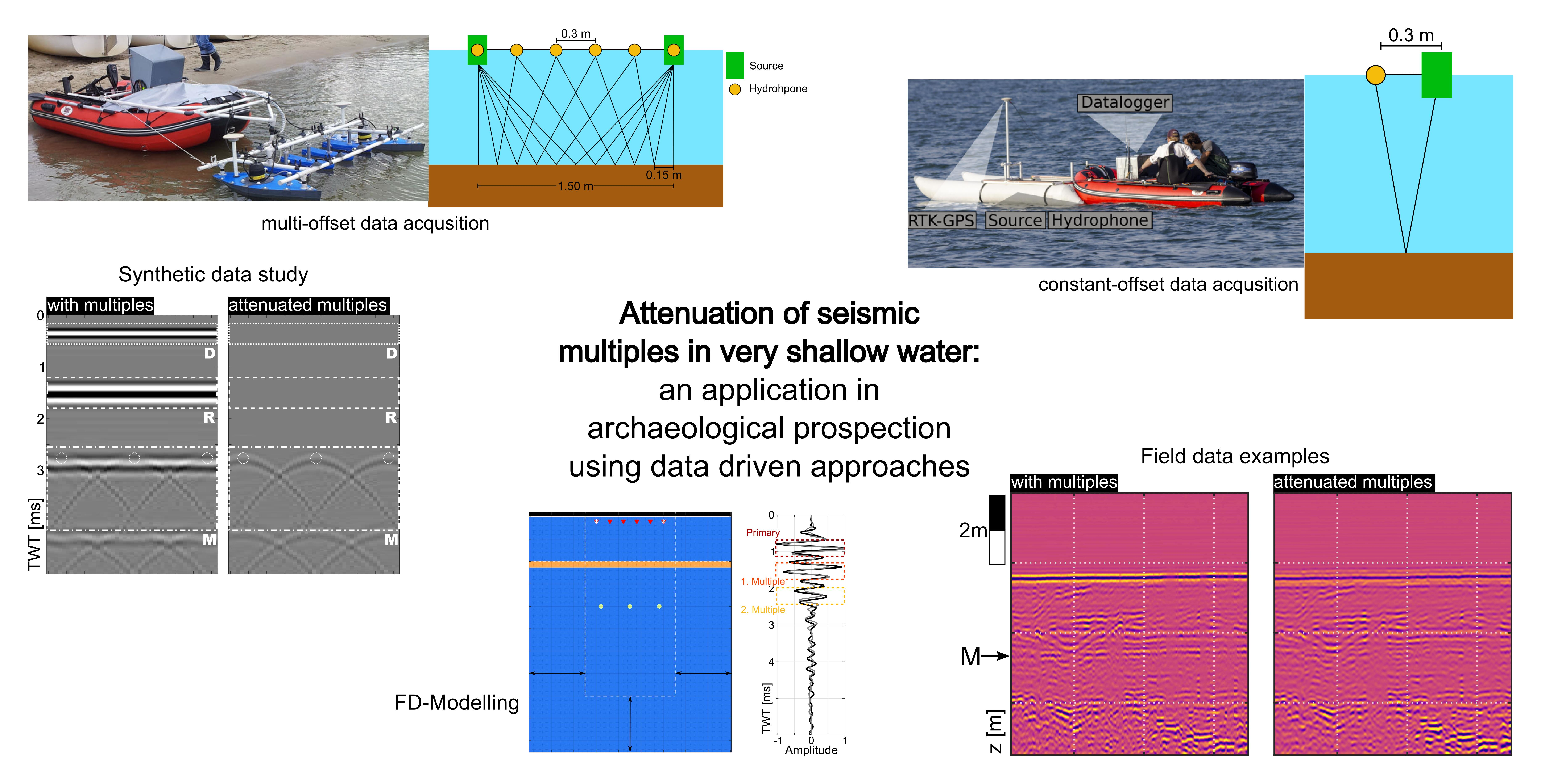
However, special difficulties arise for the application of the above-mentioned multiple suppression algorithms from the very shallow water depths investigated in geophysical and archaeological studies of the near-shore area on the one hand and from the applied reflection seismic system which differs from the systems commonly used in large scale seismic acquisition on the other hand. 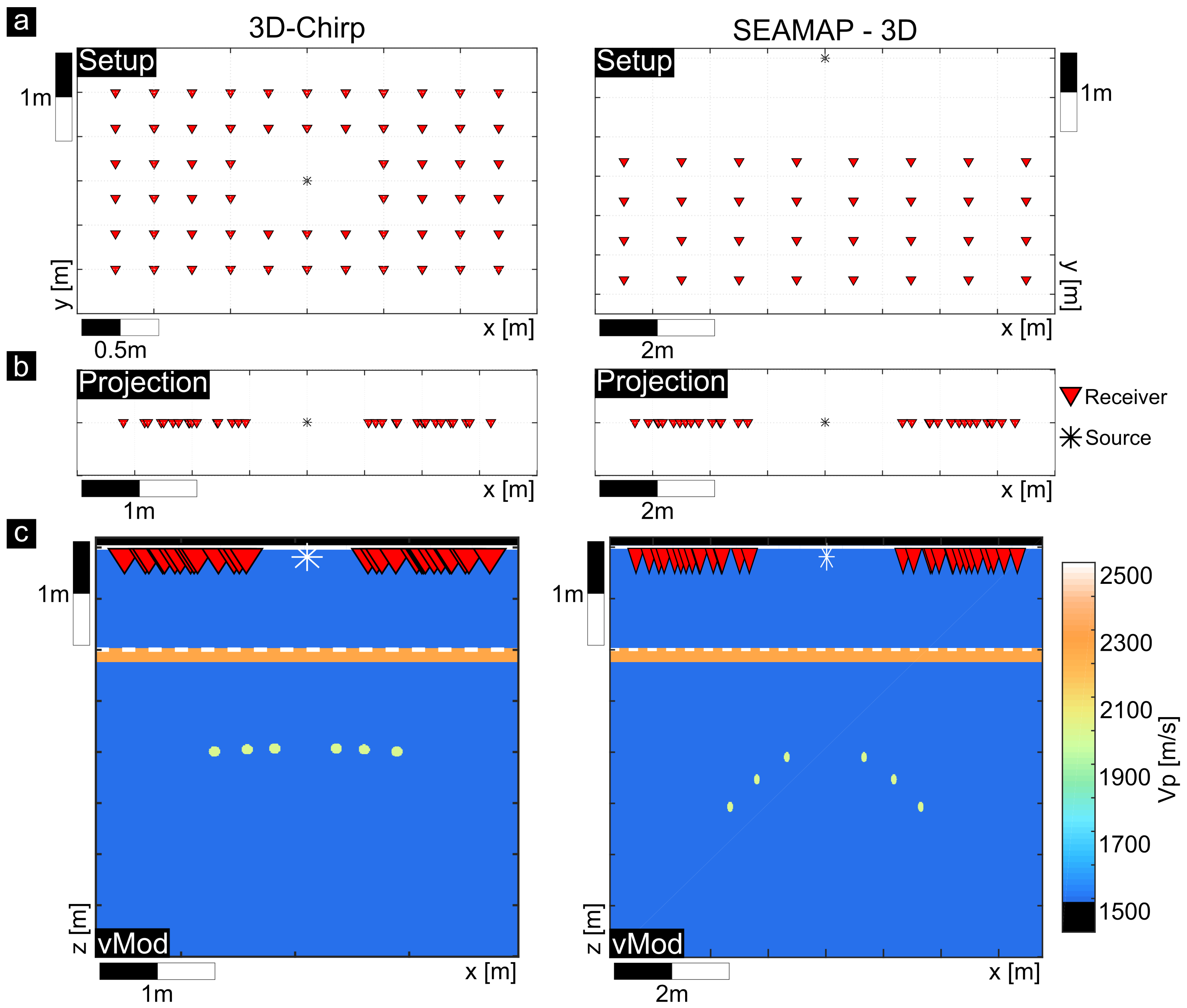The usage of the newly developed marine seismic acquisition system by [26] consisting of two pinger sources and six hydrophones, allows for an acquisition with efficient area coverage of the target sites with a 1.5 m wide swath of seismic data in a single run (Figure 1a). For profile-wise acquisition a constant-offset configuration consisting of one pinger source and one hydrophone is used (Figure 1b). Both configurations can be operated in water depth as shallow as 0.3 m and are representative for marine seismic archaeological prospection in terms of high-resolution few-meters-3D systems (e.g., 3D-chirp [27,28], SEAMAP-3D [29,30], SES quattro [10]) and single beam sediment echo sounders e.g., [31,32]. In contrast to large scale seismic acquisition systems, the system allows only for single coverage of the subsurface. Furthermore, solely near, but no large offsets can be acquired, this means that in the case of typical water depths minimum offsets correspond to about $\raisebox{1ex}{$1$}\!\left/ \!\raisebox{-1ex}{$20$}\right.-1$ and maximum offsets to $\raisebox{1ex}{$1$}\!\left/ \!\raisebox{-1ex}{$5$}\right.-3$ times the water depth. In contrast to this, the data acquired by large scale seismic investigations usually contain large offsets as well as a multi-fold coverage of the subsurface reflection points. Not only the offset range and the water depth, but also the frequency ranges of high-resolution marine seismic few-meters-3D systems are different from large scale seismic acquisition systems. The ratios between water depth and frequency, as well as maximum offset and frequency is typically less than 1 for systems applied in marine seismic archaeological prospection, whereas they are greater than 1 for typical setups in large scale seismic acquisition. The ratio between maximum offset and water depth is smaller than 5 for systems applied in marine seismic archaeological prospection and greater than 5 for large scale seismic acquisition systems (see Appendix A). Archaeology is usually buried only a few meters below the water bottom and the water depths for harbor research in the near-shore area are usually shallow leading to multiples interfering with primaries reflected from archaeology or layer boundaries associated with early landscape stratigraphy. Apart from the acquired offsets and coverage, the effectiveness of classical multiple removal methods is reduced as simple assumptions made be these methods are violated. These include the periodicity of multiples, roughness of the water bottom, horizontal stratification of subsurface reflectors, sufficient move-out along with possible separation of primaries and multiples, as well as the source-receiver offset in relation to the water depth.

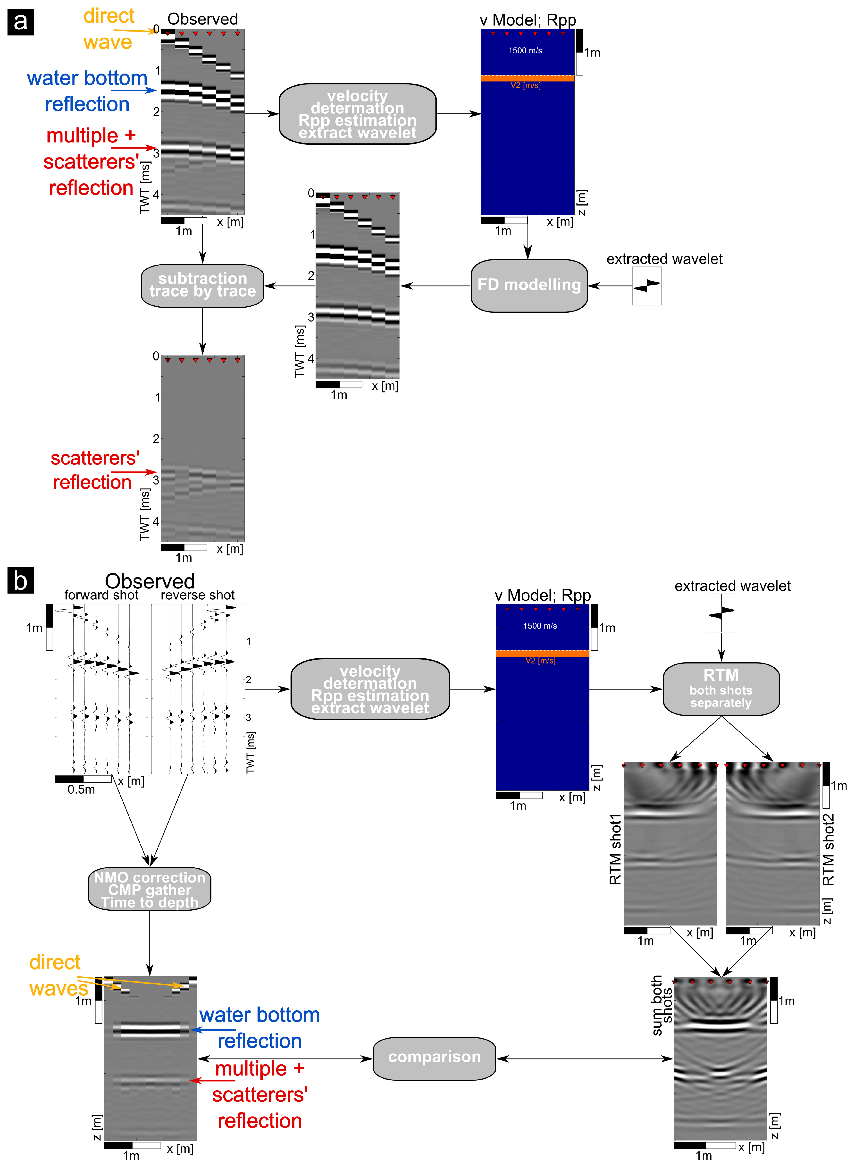
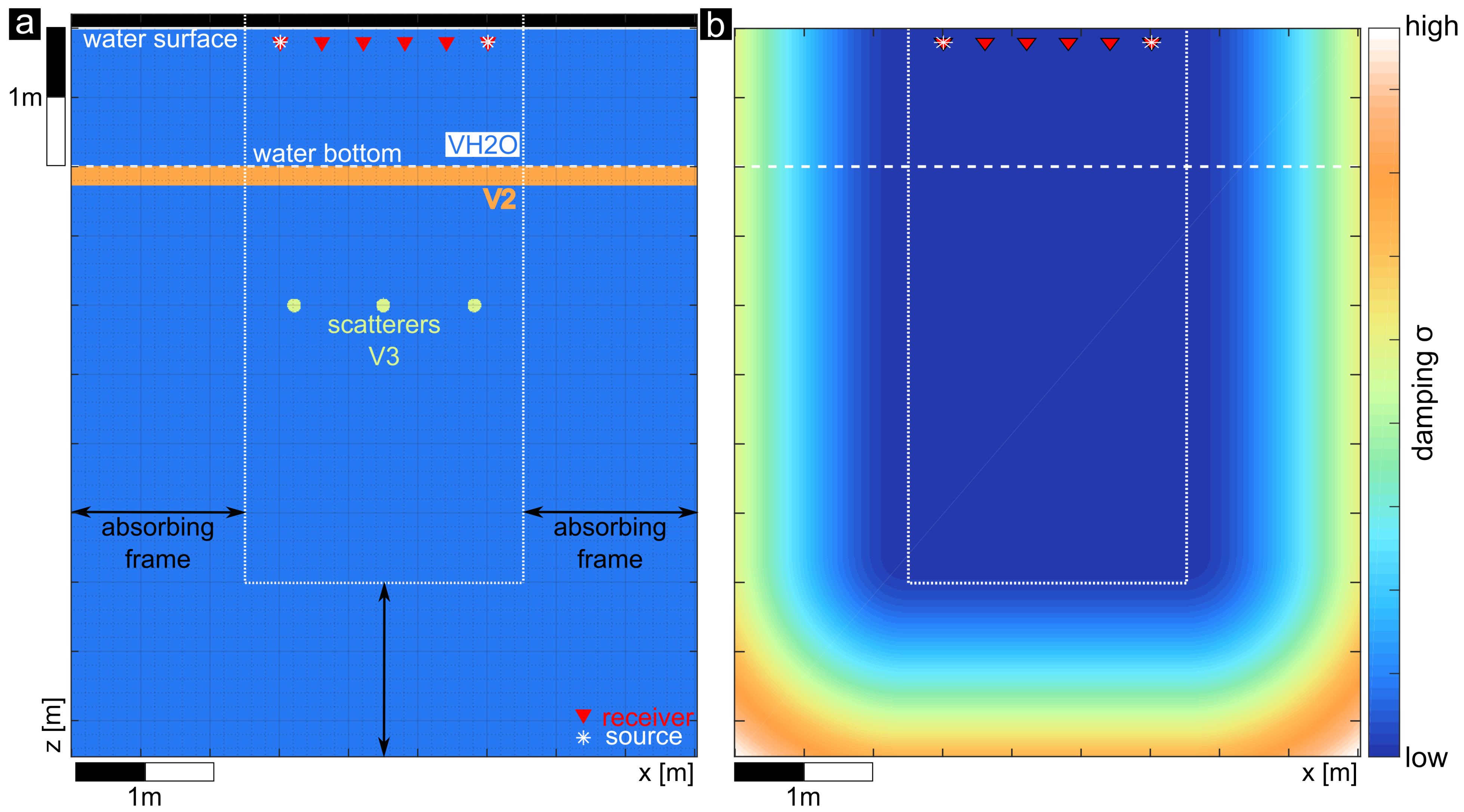
As all these factors limit the applicability of classical methods, we evaluate two model-driven approaches to remove water-layer multiples for pre-defined constant-offset as well as multi-offset synthetic test scenarios of shallow water archaeological prospection as accessible by the above-mentioned systems in the present study. In order to place these approaches in context, the results are compared with those of common multiple attenuation methods, that are usually applied in large scale seismic acquisition. In particular the following aspects and questions will be addressed:

• Applicability of both approaches to data acquired using our multi- as well as constant-offset systems tested with synthetic data sets.
• How do uncertainties in the determination of models, e.g., water depth and seafloor reflection coefficients influence multiple attenuation?
• How do these approaches perform compared to common methods such as Predictive Deconvolution and SRME concerning multiple removal efficiency, preparation and computation time as well as applicability in shallow water with available system setups?

The applicability of both approaches and common methods are further tested and compared for synthetic data with the 3D-Chirp and SEAMAP-3D setups. Last, the suggested approaches are applied to two field data sets recorded using the acquisition system PingPong and a constant-offset single channel setup system.

2. Materials and Methods

In the present study we applied two model-driven approaches to reduce the energy of water-layer multiple reflections with respect to primary reflections, which both involved forward modeling of the acoustic wave field. We chose the following multiple suppression approaches, because they are on the one hand data-driven, which means very little a-priori information is needed, that moreover can be extracted from the data itself, and on the other hand, they can be easily applied without the need for any commercial software as they rely solely on wave field modeling. Furthermore, in the second approach, the multiples are treated as signal rather than noise; therefore, two of the basic categories of multiple suppression methods are covered and in addition a depth migrated section is obtained. Both approaches are explained in detail in the following. As the presented demultiple methods needed a proper but fast full-wavefield forward modeling approach we used an FD solution of the acoustic wave equation. This includes the estimation of a velocity model together with the determination of the water bottom reflection coefficient $R_{pp}$ from the data itself. Finally, the demultiple methods were tested using field and synthetic data sets for the multi- as well as the constant-offset configuration in very shallow water and compared to two traditional suppression methods (Predictive Deconvolution and SRME).

2.1. Preliminary Considerations: Forward Modeling and Model Determination

The presented multiple attenuation methods needed a proper forward modeling approach of the wavefield, for which we used an explicit FD solution of the acoustic wave equation:

$$\frac{{\partial }^{2}p}{\partial x^2}-\frac{1}{v^2}·\frac{{\partial }^{2}p}{\partial t^2}=0,$$

(1)

with x being the coordinate vector, t the time, p the pressure field and v the seismic P-wave velocity. To include a viscous component with a constant quality factor Q, a damping term was inserted into Equation (1):

$$\frac{{\partial }^{2}p}{\partial x^2}-\frac{1}{v^2}·\frac{{\partial }^{2}p}{\partial t^2}-\frac{\sigma }{v^2}·\frac{\partial p}{\partial t}=0,$$

(2)

with

$$\frac{\sigma }{v^2}=\frac{2\pi f_c}{v^{2}Q}\Rightarrow \sigma =\frac{2\pi f_c}{Q},$$

(3)

where $\sigma$ is the damping factor, $f_c$ the central frequency and Q represents the quality factor for attenuation. We choose $Q=1000$, representing the common value for seawater. This approximation sufficiently describes amplitude attenuation effects but does not consider dispersion by attenuation. The FD solution of Equation (2) in 2D as Standard Linear Solid is the core of the forward modeling. A 2nd order explicit FD solution in 2D with a central operator is used to calculate the wavefield. For further details, see Appendix B.

Forward modeling came along with the need of a velocity model, which was determined directly from the data (see Appendix D). The water depth z was estimated by picking the time of the maximum amplitude ($t_{A_{max}}$) of the water bottom reflection and applying the seismic water velocity ($v_{H_{2}O}$) to calculate the depth. Test migrations using different velocities in the typical range were applied to determine the optimum seismic water velocity.

The contrast in seismic impedance at the water bottom was given by the reflection coefficient $R_{pp}$, which was dependent on the velocity as well as on the density of the upper and lower medium (Equation (A10)). The reflection coefficient at the water bottom was calculated from the data by the ratio of the spreading corrected maximum amplitude of the water bottom reflection $AR$ and the spreading corrected direct wave $AD$ at nearest offset (see Appendix C). Especially in the shallow marine area, the contrast in seismic impedance was mainly influenced by a change in density and not by a change in seismic velocity. We observed that the velocity in the sediment was not noticeable higher than the seismic velocity in water. This was further supported by the literature values for velocity and density for water and marine sediments e.g., [33,34,35]. The typical range for seismic velocity in marine and fresh water sediments was 1500–1700 m/s, whereas the variability for density changes from water to sediment was considerably larger ranging from 1000 kg/m³ for water to 1800 kg/m³ for marine, fluvial, and limnic sediments (e.g., gravel, sand, silt, clay, peat). Bulk modulus and density could be used in modeling, but leaves us with two variables, though we chose this approach, where the reflection coefficient has to be implemented in a different way. In our models we simulated the reflection coefficient by a small layer (lamella) of higher velocity following the approach of [36] that also considered interference effects due to the lamella. Under the assumption that the density did not change, i.e., ${\rho }_1={\rho }_2=const$, the reflection coefficient was given by

$$R_0=\frac{v_2-v_1}{v_2+v_1}.$$

(4)

Since $v_1$ and $R_0$ could be derived from the data itself, the velocity $v_2$ of the lamella was obtained by rearranging Equation (4):

$$v_2=v_1·\left(\frac{1+R_0}{1-R_0}\right).$$

(5)

The thickness d of the lamella was then calculated as follows:

$$\frac{2·\omega ·d}{v_2}=n·\pi ,$$

(6)

with n being even to exclude interference effects. Rearranging Equation (6) with $n=1$ and the angular frequency $\omega =2·\pi ·f$, it is:

$$\frac{2·\omega ·d}{v_2}=\frac{2·2·\pi ·f·d}{v_2}=1·\pi \Rightarrow d=\frac{v_2}{4·f}.$$

(7)

2.2. Applied Model-Driven Multiple Attenuation Methods

2.2.1. Method A: Prediction and Subtraction

In the first tested multiple suppression approach synthetic seismograms were modeled based on Equation (2) using a previously derived velocity model with the water bottom and the water surface as only reflecting boundaries in the model and a source wavelet which was forward propagated through that velocity model. The resulting synthetic seismograms were then subtracted trace-by-trace from the field data after an amplitude adaption (Figure 2a). The maximum amplitude of the first water bottom multiple was set to 1 for each trace in the field as well as in the synthetic data. Small time variations between the field and the corresponding synthetic traces due to e.g., small water depth variations were calculated by cross-correlating the traces. The computed lag was then used to correct small time shifts. For constant-offset data, each shot was modeled separately and the modeled wavefield was saved at the receiver position. The modeled wavefield in case of multi-offset data was saved at each of the six receiver positions for each shot.

2.2.2. Method B: RTM-Deco

The second tested approach consisted of a pre-stack migration and is based on the method suggested by [24]. Applying the concept of forward and inverse wavefield extrapolation followed by Claerbout’s imaging principle [37], multiple energy was reduced. This approach was realized as a cross-correlation of the modeled shot and receiver wavefields for each time step. Multiples do not contribute to cross-correlation imaging and can be removed by an additional deconvolutional filter [38]. This method was implemented as a reverse time migration (RTM) algorithm including a 1D deconvolution imaging condition (Equation (8)). Similar to method A, a source wavelet was forward propagated from the source point into the subsurface through a velocity model, but additionally the reflected wavefield was also back propagated into the ground from the receiver plane. Both wavefields are modeled using the FD solution of the acoustic wave equation (Equation (2)). At each subsurface position, the reflector image was obtained by extracting the zero-lag sample of the deconvolved extrapolated wavefields. After [39], the ability of the 1D deconvolution imaging condition to suppress multiples is limited in 2D and 3D cases, but multiples are still weakened.

In the case of data from the multi-offset configuration, the shots from the left and right source were migrated separately with the 1D imaging condition and then both migrated images are summed to obtain the resulting image (Figure 2b). In the case of constant-offset data, each shot was also migrated separately, and the resulting image was obtained by summing all migrated images at the end for the whole profile. The 1D deconvolution imaging condition $I_{D_{1D}}$ was defined as

$$I_{D_{1D}}(x,y,z)=\frac{1}{2\pi }\sum _{x_{src}}\left(\sum _{\omega }\frac{U(x,y,z,\omega ;x_{src})D^{*}(x,y,z,\omega ;x_{src})}{D(x,y,z,\omega ;x_{src})D^{*}(x,y,z,\omega ;x_{src})+ϵ}\Delta \omega \right),$$

(8)

with the horizontal source position $x_{src}$ and the angular frequency $\omega$. x and y are the in-line and cross-line spatial coordinates, respectively, and z is defined as the positive downward depth. U and D are the upgoing or reflected and downgoing or incident wavefields. The conjugate of D ($D^{*}$) was multiplied with both the top and bottom of the quotient to assure that the denominator was real and non-negative. To further ensure that the denominator was non-zero, a small real value $ϵ$ was added.

2.3. Traditional Methods Applied for Comparison

2.3.1. Basic Method 1: Predictive Deconvolution

Predictive Deconvolution is the oldest way of suppressing multiples, as these are events that have a strong periodic character [11]. It makes use of the assumption, that multiple reflections appear in a repetitive pattern, while primary reflections do not; therefore, the two can be separated based on statistics [40,41]. In order for this method to work properly, primaries are needed. In its simplest form, a time shift is applied to each primary on each trace followed by amplitude scaling and a phase reversal, as amplitudes of multiples alternate in sign. If the seismic trace is shifted by the period of reverberations, then each primary will match in time with its first-order multiple and each multiple will match in time with the next higher-order multiple. Amplitude matching is achieved by scaling the shifted version with the reflection coefficient of the water bottom. After summing the original and the shifted records, only primary reflections will remain [42].

Predictive deconvolution was applied to the synthetic constant-offset and multi-offset data sets using the VISTA 2018 Desktop seismic data processing software (Schlumberger). The data were first bandpass filtered with corner frequencies of 1000, 1500, 7000, and 8000 Hz, followed by a top mute of all signal above the water bottom reflection. A spiking deconvolution (standard Wiener Levison algorithm) was applied with an operator length of 0.75 ms, equaling one and a half times the length of the wavelength at the water-bottom reflection, the design window was centered around the water bottom reflection (

Table 1. Overview of applied parameters for spiking deconvolution in VISTA seismic data processing software.

Water Depth [m]	Design Window [ms]
1.0	1.2–1.8
0.5	0.6–0.9
0.3	0.4–0.6
0.25	0.3–0.45

). Afterwards, the data were again bandpass filtered. The multiples were suppressed by applying a predictive deconvolution with a prediction lag equal to the lag between the multiples or the period of reverberations, followed again by a bandpass filter (

Table 2. Overview of applied parameters for predictive deconvolution in VISTA seismic data processing software.

Water Depth [m]	Prediction Lag [ms]
1.0	1.0
0.5	0.5
0.3	0.3
0.25	0.25

).

2.3.2. Basic Method 2: Surface-Related Multiple Elimination

The method of SRME is a data-driven method that makes use of the idea that a first-order multiple consists of two primary reflections which are connected at the surface reflection point. This allows to construct multiples by combining two primary reflections available in the data and avoids the need for subsurface information. Each multiple is taken as the convolution of two sub-events, e.g., two primary reflections, and can be constructed by the convolution of sub-events [42]. Therefore, total field $x\left(t\right)$ with all surface multiples can be describes as a series of the impulse field of the subsurface $x_0\left(t\right)$:

$$x\left(t\right)=x_0\left(t\right)-x_0\left(t\right)\ast x_0\left(t\right)+x_0\left(t\right)\ast x_0\left(t\right)\ast x_0\left(t\right)-....$$

(9)

The implicit relation for the impulse response of the subsurface with all multiples is given by:

$$x\left(t\right)=x_0\left(t\right)\ast [\delta \left(t\right)-x_0\left(t\right)]=x_0\left(t\right)-x_0\left(t\right)\ast x_0\left(t\right),$$

(10)

with $\delta \left(t\right)$ being the original source. Thus, all surface-related multiples can be obtained by convolving the primaries with the total reflected field. The multiple-free field can therefore be obtained from the total field as a series of convolutional products [42]:

$$x_0\left(t\right)=x\left(t\right)+x\left(t\right)\ast x\left(t\right)+x\left(t\right)\ast x\left(t\right)\ast x\left(t\right)+....$$

(11)

SRME was applied to the synthetic constant-offset and multi-offset data sets using the VISTA 2018 Desktop seismic data processing software (Schlumberger). First, the seismic data were bandpass filtered between the corner frequencies of 1000, 1500, 7000, and 8000 Hz, followed by a top mute of all signal above the water bottom reflection. Using the Back-End-Mute option, points just below the water-bottom reflection were picked and stored to the headers. Then, the SRME prediction step was performed to predict the multiples for all shots for a maximum frequency of 8 kHz and a normal-moveout (NMO) velocity of 1500 m/s. The data with attenuated multiples were then computed using adaptive subtraction in the frequency domain with a maximum frequency of 9999 Hz. The start times were read from the headers and equal the time picks below the water-bottom reflection. With the SRME window following option enabled, the moving window size was adjusted to the depth of the water bottom. An overview of the used parameters can be found in

Table 3. Overview of applied parameters for the adaptive subtraction step in VISTA seismic data processing software.

Water Depth [m]	Start Time of Applied Filter	Moving Window Size [ms]	Operator Length [ms]
1.0	2.5	3	1
0.5	1.25	2	1
0.3	0.83	2	1
0.25	0.625	2	1

.

2.4. Test Data

2.4.1. Field Data

About 45 marine seismic reflection data sets were recorded at 15 different locations throughout the SPP1630 project using either the multi-offset or the constant-offset acquisition configuration. The water depth generally varied between 0.5 m and 5 m and in some cases depths greater than 10 m occur (e.g., [6,26]). Different subsurface lithologies and sediments are found depending on the site including gravel, as well as sand, peat, silt, or clay, leading to different reflection coefficients at the water bottom. The observed reflection coefficients ranged from $R_{pp}=0.2$ to $R_{pp}=0.8$, with $R_{pp}=0.4$ being the most common value.

The multiple attenuation approaches were tested on two field data sets. Field data set 1 was recorded close to a Pier in Puck, Poland, where the remains of ship wrecks were expected below a cover of sediments. The data were acquired using the PingPong system perpendicular to the shore. Additionally to one constant-offset profile of this data set, one multi-offset section representing one shot location along the profile was used to demonstrate the applicability of approaches A and B to a data set acquired in very shallow water with a water depth ranging from 0.5 m to 0.54 m. The pre-processing of the data included bandpass filtering using a Butterworth filter opening at 1 kHz to 2 kHz and closing from 6 kHz to 7 kHz, trace normalization, and resampling according to the needs of modeling concerning the time step. A NMO correction with a water velocity of 1500 m/s was applied to the multi-offset data. The velocity model for the FD modeling was obtained following Equation (A15) for the water depth estimation and Equation (A16) for the determination of the reflection coefficient at the water bottom, from which the velocity contrast and the thickness of the lamella were calculated by Equations (A12) and (A13). This yielded a water depth of about 0.5 m with a reflection coefficient at the water bottom of $R_{pp}=0.4$, equaling a velocity contrast between 1500 m/s and 2250 m/s.

Field data set 2 is an example for the typical contrast in acoustic impedance and was recorded in the German North Sea between the Islands of Pellworm and Nordstrand, where the remains of a medieval dike system are located [43]. The data were recorded using the constant-offset configuration. Method A was applied to one section of a profile, where the first water-layer multiple was interfering with the primary reflection of the dike’s remains. The pre-processing of the data included bandpass filtering using a Butterworth filter opening at 1 kHz to 2 kHz and closing from 6 kHz to 7 kHz, spiking deconvolution, automatic picking of the seafloor reflection and smoothing with a moving average of 120 traces to suppress wave motion followed by a semblance-based coherence filter [44], trace normalization, and geometrical spreading correction. The data were migrated using Stolt migration [45] with a constant velocity of 1480 m/s and then resampled according to the needs of modeling concerning the time step with $dt={10}^{-6}s$. The velocity model for the FD modeling was obtained following Equation (A15) for the water depth estimation and Equation (A16) for the determination of the reflection coefficient at the water bottom, from which the velocity contrast and the thickness of the lamella were calculated by Equations (A12) and (A13). This yielded a water depth of approximately 2.15 m to 2.52 m along the profile with a mean reflection coefficient of $R_{pp}=0.45$.

2.4.2. Synthetic Test Data

The synthetic model for both multi- and constant-offset scenarios was derived based on the typical values and characteristics found at various test sites. The geophones and sources were distributed as found in the PingPong configuration for multi-offset and with a source-receiver spacing of 0.3 m for the constant-offset acquisition system (Figure 1). The water depth was set to either 0.25 m, 0.3 m, 0.5 m, or 1 m with a water velocity to 1500 m/s. The total model depth was set to 4 m. The left and right sources were put 0.25 m from the edge to avoid edge effects. The whole model was surrounded by an absorbing boundary frame with a width of 1.25 m. In the absorbing frame the waves were damped by the damping coefficient $\sigma$. At the top boundary free surface conditions were met by a high velocity contrast using the seismic velocity of air ($v_{air}={10}^{-6}$ m/s). The test scenarios for the multi-offset and constant-offset configurations included three shallow scattering objects, one in the middle of the acquisition geometry and one on each side (Figure 3). The two way travel time of the reflections from the scatterers corresponded to the theoretical travel time of the seafloor multiple and were masked by it. The seismograms of the synthetic test models were generated using a 2nd order FD modeling scheme of the acoustic wave equation (Equation (2)), which was also applied in the multiple suppression approaches.

3. Results

3.1. Results of the Synthetic Study

In each synthetic test scenario, the data were contaminated by water-layer multiples which mask the primary reflections of three scattering bodies in the subsurface (Figure 4 and Figure 5, first column). To attenuate the multiples, methods A and B were applied to the data set. In case of the constant-offset section, only method A was applied to the data. To put the multiple attenuation result of the applied approaches into a context, the results were compared to two established traditional methods.

3.1.1. Constant-Offset Section

Figure 4 shows the result after the application of Predictive Deconvolution, SRME, and method A to synthetic test case scenarios with the constant-offset configuration for water depths between 1.0 m (Figure 4a) and 0.25 m (Figure 4d). With decreasing water depth, the time between the water bottom primary (R in Figure 4) and first water-layer multiple (M in Figure 4) decreased. For a water depth smaller than 0.5 m, the primary and multiple interfered (Figure 4c,d). The first water-layer multiple was attenuated to a great extent by all applied methods, but some energy of the second multiple remained in the data. The primary reflections of the scattering objects (R2 in Figure 4), formerly hidden by the multiple, were noticeably enhanced, especially with method A. When the traditional methods were compared to method A, it could be seen that SRME as well as Predictive Deconvolution also attenuated the reflection of the scattering objects, which was not the case for method A. Moreover, as the water depth decreased, the amount of multiple energy attenuated by the traditional methods decreased (

Table 4. Overview of attenuated multiple energy in percent compared to the reflection for each applied method for the synthetic constant-offset test scenarios.

Water Depth [m]	Pred. Decon.	SRME	Pred. and Sub.
1.0	97.5%	86%	>80%
0.5	91%	80%	>80%
0.3	90%	58%	>80%
0.25	50%	29%	>80%

), whereas it was constant for method A. At a water depth of 1.0 m, the multiple energy was reduced by 97.5% and 86.0% compared to the reflection from the scatterers by applying Predictive Deconvolution and SRME, respectively. Method A achieved a reduction of more than 80%. The values stating the percentage of attenuated multiple energy for shallower water depths for all applied methods are stated in Table 4.

3.1.2. Multi-Offset Section

Figure 5 shows the result after the application of Predictive Deconvolution, SRME, and methods A and B to synthetic test case scenarios with the multi-offset configuration (PingPong) for water depths between 1.0 m (Figure 5a) and 0.25 m (Figure 5d). With decreasing water depth, the time between the water bottom primary (R in Figure 5) and first water-layer multiple (M in Figure 5) decreased. For a water depth smaller than 0.5 m, the primary and multiple interfered. The multiple was attenuated by all applied methods and the reflections of the scattering objects (R2 in Figure 5) were enhanced, but when the traditional methods were compared to method A, it could be seen, that SRME as well as Predictive Deconvolution also attenuated partly the reflection of the scattering objects. Moreover, as the water depth decreased, the amount of multiple energy attenuated by methods A and B was constant, whereas it decreased for the traditional methods (

Table 5. Overview of attenuated multiple energy in percent compared to the reflection for each applied method for the synthetic multiple-offset test scenarios.

Water Depth [m]	Pred. Decon.	SRME	Pred. and Sub.	RTM
1.0	97%	86%	>80%	>60%
0.5	90%	85%	>80%	>60%
0.3	88%	67%	>80%	>60%
0.25	70%	63%	>80%	>60%

) and artifacts were introduced. After the application of method B, there was still multiple energy, but the primary reflections of the scattering objects, especially that in the center, were strongly enhanced and distinguishable. In the case of a water depth of 1.0 m, the multiple compared to the reflected energy was reduced by 97.0% and 86.0% using Predictive Deconvolution and SRME, respectively. With method A the multiple reflection reduced by more than 80% and with method B by 60%. The values stating the percentage of attenuated multiple energy for shallower water depths for all applied methods are stated in Table 5.

3.1.3. Additional Considerations

The above shown results of method A and B represented the ideal circumstances, where the water depth, the velocity model, and the source wavelet were known. As all these parameters were estimated for model generation, their quality may have had an effect on the final result.

The effect of incorrect water depth estimation was investigated. Therefore, small scale variations of the water depth were included in the velocity model for synthetic data generation (Figure 6a). For forward modeling, the water depth was set to 1.0 m, equaling the mean water depth determined from the synthetic test data. With the Prediction and Subtraction approach, about 80% of the first water-layer multiple was suppressed. With method B the scattering objects were enhanced.

Water-layer multiples were truly periodic only in a 1D medium and a true 3D medium always led to a worse attenuation by the traditional methods as they rely on this simple assumption. In the multi-offset configuration offsets were small, and as the water velocity was low, the multiple reflection bent towards the normal, which allowed the traditional methods to still perform well. If the water bottom had a slope of circa $4.5\%$ (Figure 6b), the multiple energy suppressed by methods A and B was about the same (>80%, 65%) as in the case with a flat water bottom.

To investigate the effects of incorrect water bottom reflectivity determination on the result of method A, the velocity/impedance contrast at the water bottom was varied between 25 and 100% of the true reflectivity ($R_{pp}=0.1-0.4$, $R_{pp}^{True}=0.4$) for the multi-offset model (Figure 6c) with a water depth of 1.0 m. More than 80% of multiple energy compared to the scatterers was removed in the case of using the true water bottom reflectivity for predicting the multiples. If a value of less than 80% of the true reflectivity was used less than 50% of the multiples are attenuated.

3.2. Application of Multiple Suppression Methods to Other Systems Applied in near Surface and Archaeological Prospection

In order to classify the effectiveness and transferability of the evaluated methods, they were applied to synthetic data modeled using FD modeling according to Equation (2) for the configurations of other high-resolution seismic reflection systems used in archaeological prospection. The source-receiver-offsets of the 3D-Chirp system [27] as well as the SEAMAP-3D system [29] were projected from the x-y-plane (Figure 7a) to the x-plane (Figure 7b) and synthetic velocity models comparable to the test data cases were generated (Figure 7c). Again, the scattering objects were included at depths corresponding the theoretical travel time frame of the first water-layer multiple. In the synthetic seismic sections (Figure 8), the strong water bottom reflection and two water-layer multiples were seen, which covered the reflections from the scattering objects.

The NMO corrected synthetic test data is shown in Figure 8 (column 1). For comparison between the applied multiple attenuation methods, all data were NMO corrected. Both the applied methods A (Figure 8, column 4) and B (Figure 8, column 5) were capable of reducing the multiple energy by more than 50% in ideal circumstances, provided that the source wavelet was known and the water depth and velocity model were determined correctly. Compared to the standard methods (Predictive Deconvolution: Figure 8, column 2; SRME: Figure 8, column 3) this was slightly less, as more than 85% of the multiple energy was suppressed by these approaches. However, the application of the standard methods also reduced the reflection of the scattering objects. Especially, the application of method A enhanced the primaries of the scattering objects for both 3D systems and thereby demonstrated the transferability of the Prediction and Subtraction approach to other system configurations.

3.3. Results of Tests with Field Data Sets

3.3.1. Field Data Set 1: Puck, Poland

The applicability of approaches A and B to a field data set acquired in very shallow water was demonstrated for field data set 1. The multi-offset section represents one shot (S260) recorded with the PingPong acquisition system, it was centered in the constant-offset profile extracted from the data. Both the constant-offset and multi-offset section showed a strong water bottom reflection and its water-layer multiples (Figure 9a and Figure 10a). The water-layer multiple (Figure 9, B; Figure 10, M) was attenuated with all methods. The results of Predictive Deconvolution (Figure 9b and Figure 10b) and SRME (Figure 9c and Figure 10c) showed that nearly all energy was eliminated, whereas a small amount of multiple energy remained in the Prediction and Subtraction result. Compared to the results of method A (Figure 9d and Figure 10d) and B (Figure 9e), not only multiple energy, but also primary energy that was masked by the multiple reflection, was attenuated by the application of the traditional methods. This was clearly seen in the Prediction and Subtraction as well as in the RTM-Deco result, where these reflections were enhanced. Further, in the multi-offset section, SRME attenuated reflection C in a depth of approximately 3.0 m.

When comparing the result of method A with Predictive Deconvolution and SRME for the constant-offset profile, one could see that especially in the cases of Predictive Deconvolution and SRME a large amount of multiple, but also primary energy below the water bottom primary was attenuated. After the subtraction of the modeled multiples, a distinct reflector got strongly enhanced (Figure 10, A), which was not seen in the results of the Predictive Deconvolution and SRME multiple attenuation. The multiple attenuation together with the enhancement of the shallow reflector is highlighted in the extracted details displayed in Figure A2 and Figure A3 (Appendix E).

In Figure 11 the traces for shot 260 of the constant-offset section were compared with the observed data for each applied method. Further, the forward modeled trace which was subtracted in method A is compared to the measured data (Figure 11d). The modeled travel times of the water bottom primary and multiple reflection showed only little deviations and the waveform of the modeled data matched that of the measured data well. The final data showed only some remaining reverberations of the primary and multiple after the subtraction of the modeled from the measured data. The remaining energy at the time of the first multiple belonged to the reflection highlighted in Figure 10. The exemplary traces for the traditional methods showed only small remaining multiples.

3.3.2. Field Data Set 2: Wadden Sea, Germany

Method A was also applied to one 67.7 m long section of a profile from field data set 2. In the field data (Figure 12a), the water-layer multiple interfered between 10 m and 30 m along the profile with reflections from the remains of an ancient dike at a depth of 4.5 m to 5.0 m (Figure 13). After the subtraction of the modeled from the observed data, the multiple was clearly attenuated and the reflection of the dike was enhanced (Figure 12b and Figure 13b). For comparison the sections with attenuated multiples after the application of Predictive Deconvolution (Figure 12c and Figure 13c) and SRME (Figure 12d and Figure 13d) are shown.

Both the traditional methods were able to attenuate the multiples by 56% and 52%, respectively. Compared to the multiple attenuated result of the Prediction and Subtraction method, this was slightly less, as approximately 70% of the multiple energy could be attenuated with method A. Furthermore, the Predictive Deconvolution as well as SRME also attenuated some primary energy in the time range of the first water bottom multiple around 6 ms/4.5–5.0 m, as highlighted in Figure 14. The results after the application of each multiple attenuation method were subtracted from the observed data to show what each approach attenuated. While method A only subtracted some minor primary signal along with the primary water bottom reflection, the traditional methods also attenuated the main primary reflection of interest. In particular by SRME a large amount of the measured signal was removed from the data. Further, it is shown that with method A all reflections related to the water bottom were effectively predicted and removed from the observed data.

4. Discussion

4.1. Limitations of the Applied Methods

Despite the good attenuation results obtained by the application of methods A and B to both synthetic test and field data, there are some limitations that should be discussed. The first, and most serious limitation is the long time required for the computation of the wavefields in the modeling step. Compared to the traditional methods, the computational costs are considerable higher for both the evaluated methods. The method of predictive deconvolution is fastest (in our case $n·1$ s order of magnitude for a test data set), followed by the application of SRME, which was slower by a factor of 10 ($n·10$ s in our cases). However, the full time needed for the SRME processing is longer than the computation time of one run because considerable additional time is required for parameter testing for the adaptive subtraction step. Compared to SRME the “Prediction and Subtraction” approach presented here is again slower by a factor of 10, needing about one to two minutes in our case per shot gather, comparable to the “RTM-deco” approach ($n·1$ min for the test cases).

Apart from this, other factors may limit the quality of the multiple attenuation by methods A and B. In the determination of the velocity model, in particular both the estimation of water depth and the water-bottom reflectivity may lead to errors and deviations from the original data in the predicted multiples. Differences in amplitude and slightly different signal lengths between the measured and modeled data lead to the consequence that the multiples are not predicted completely. Furthermore, variations in reflectivity in the whole data set have to be considered. Especially in the case that the water-depth is so small that the primary and multiple reflection of the water-bottom interfere, these parameters may not be determined correctly. Last, the modeling result further could be limited by the estimated source wavelet as the true source wavelet is unknown and the multiple waveform may not be predicted correctly. As all processing steps needed in model estimation can be automated with minimal user intervention and are therefore mostly an objective procedure, a manual check of the determined model parameters is crucial. In [19,40] the limitations of similar wave-equation based multiple prediction methods are discussed. As here, the long computation time is the most severe limitation stated, among other limiting factors such as spatial aliasing, lack of near-offset data, and errors in the estimation of the water-bottom reflectivity.

4.2. Limitations of the Traditional Methods

For comparison two traditional methods were applied to the synthetic test case scenarios and the field data sets. These methods also have their limitations as the comparison shows. The most severe disadvantage of Predictive Deconvolution is that also primary events with a similar periodicity as the water-layer multiple are attenuated [46]. This was also shown by [41] where additionally artifacts are introduced by Predictive Deconvolution. With the water bottom not being perfectly flat, small variations in the reverberation period are introduced, effecting the attenuation result [42]. Furthermore, Predictive Deconvolution is limited in the case of a hard water bottom leading to a multiple amplitude being stronger than the primary, which cannot be fully attenuated. Moreover, as multiply reflected energy is truly periodic only in a 1-D medium, predictive deconvolution is most effective in such a medium [11,40]. This is rarely the case and a true 3D medium always leads to a worse attenuation. As offsets are small in the multi-offset configuration, and the water velocity is low, the multiple reflection bends towards the normal, predictive deconvolution also works quite well under these conditions [42]. Applying a NMO correction using the seismic velocity of water before predictive deconvolution, better attenuation results can be achieved. Other limitation of this method are varying water depths, resulting in small variations in the reverberation period from trace to trace along the profile as well as the multiple generating layer not being horizontal, which affects the attenuation result [40]. In the presence of noise Predictive Deconvolution can become unstable [40].

Several studies have shown that multiples are less effectively attenuated in shallow water by SRME, especially if primary energy at near offsets is missing [47]. In large scale seismic setups, the near offsets are either often not recorded or near-offset traces are noisy, resulting in a erroneous estimation of the water bottom as multiple generating boundary. The advantage of multiple prediction and attenuation using SRME and adaptive subtraction is, that no explicit a-priori subsurface information is needed [42], but knowledge about the source wavelet, which is typically not well known, and the surface reflectivity are required [20]. Therefore, an adaptive process is used to subtract the predicted multiples from the data. This adaptive subtraction procedure involves some parameter testing before an optimal result is obtained, which is (a) time-consuming and (b) partly a subjective process. For the presented test scenarios and field data examples, both the attenuation by SRME and Predictive Deconvolution achieve very good results concerning the multiple elimination, but also attenuate some primary signal of interest. That is very problematic as weak reflections which are masked by the multiple as it is often the case in shallow water archaeological prospection are also eliminated from data and signal of interest is lost. In e.g., [41,46] non of the applied methods or combination of methods including Predictive Deconvolution and SRME produced satisfactory results for the shallow water area investigated in these studies.

4.3. Advantages of the Applied Methods

Beside the mentioned limitations, the applied methods A and B offer some advantages compared to the traditional multiple attenuation methods, especially in the considered shallow marine area and with the used seismic acquisition systems. As shown by previously studies, the inclusion of multiples in imaging algorithms such as RTM leads to enhanced imaging of the subsurface. Moreover, both the upper and lower side of the reflector are imaged [48]. Reference [49] presented a full wavefield migration including multiples where the crosstalk from multiples are removed if the multiple-generating boundaries are included. The RTM-Deco approach has the advantage that a depth migrated section is obtained as a by-product which suites the purpose of gaining high resolution subsurface images needed for archaeological investigations, which thereby compensates the longer calculation time. As has been shown by [19] for a shallow water case with a hard complex water bottom, multiples can be accurately predicted and attenuated by numerical wave extrapolation and subtraction. In addition, wavefield prediction methods are able to suppress not only water-layer, but all types of multiples and do not coincidentally attenuate primaries with stacking velocities close to the multiples as well [40]. As shown in this study, the applied Prediction and Subtraction approach is able to predict and attenuate the multiples even in very shallow water with a water depth less than the smallest source-receiver offset (<0.3 m). Similar to SRME, methods A and B are both data-driven and only need little a-priori information about the medium such as the source wavelet and the water-bottom reflectivity, which can be effectively derived with little errors from the data itself.

4.4. General Application of the Applied Methods

As shown by the field data examples, limitations in the multiple prediction given by incorrect water depth and source wavelet estimation can be corrected in post-processing in the subtraction process. Small variations and deviations in the water depth leading to time differences between the observed and predicted water bottom primary and multiple reflections can be calculated by cross-correlating the observed and modeled data trace by trace and using the computed lag to shift the modeled data. An error in the estimated reflectivity of the water bottom leads to a deviation in the amplitudes. By normalizing the modeled by the observed bottom water reflection, the amplitudes are adapted to each other.

Concerning the general application of all the tested methods for data acquired with the PingPong or constant-offset systems, we find that predictive deconvolution is a good first choice as multiple attenuation method, especially for zero- or constant-offset data as it can be easily applied during field work. The application of SRME is quite fast as well and achieves satisfactory results, but in our case the use of a commercial software is disadvantageous when it comes to its application during fieldwork. Especially in archaeological investigations, a first implementation during field work is often crucial as it affects further measurement decisions. The longer computation time of methods A and B complicate an application during field work. As the presented results are satisfactory concerning the multiple attenuation and very convincing regarding the enhancement of masked primary reflections as shown by the field data examples, especially the application of method A is highly beneficial in shallow water archaeological investigations.

4.5. Future Research and Improvements

Future improvements and developments could include an adaption of the modeling procedure with an inclusion of the density in the FD modeling of the acoustic wave equation to better reflect the true conditions found in the shallow water area. For method B, the implementation of a 2D instead of the applied 1D deconvolution imaging condition in the RTM algorithm could lead to a further improvement of the multiple suppression [39]. In both approaches the computation costs could be further reduced by implementing convolutional Perfectly Matched Layers [50] instead of the absorbing boundary frame as the grid size will be significantly reduced and computational resources could be saved. The source wavelet estimation could be implemented as a linearly damped, least-squares optimization problem according to the approach of [51,52], leading to an improved source wavelet for the modeling step and therefore to a better multiple prediction.

4.6. Placement in Relation to Other Geophysical Methods

High-resolution reflection seismic methods provide the possibility to investigate large areas with a resolution in the decimeter range as has been shown by e.g., [10,27,29,30]. The used multi-channel marine seismic acquisition system by [26] allows to cover large areas with 3D imaging capabilities in an adequate amount of time. In comparison, offshore magnetic gradiometry does not provide data with a depth resolution. An additional drawback is the decrease of resolution with increasing water depths due to the growing distance between the sensors and the buried targets. As far as ERT surveys are concerned, both resolution and penetration depth are lower compared to reflection seismics. This has been shown by [6], where the spatial resolution of different setups was investigated. They show that with submerged electrodes stone settings of a width of 0.5–1 m can still be located within the uppermost 4 m below the water bottom. With a floating electrode setup, the stone settings have to be larger than 2 m to be detected. Concerning the processing of the data, additional considerations must be be taken into account for each method when applied in shallow water. Since all methods are limited in their application and reach their limits under certain conditions, a combination of different methods should generally be applied to obtain the best possible result.

Compared to other geophysical prospection methods applied in shallow water-covered areas seismic methods convince especially through their high resolution. The problem of water-layer multiples interfering and covering the structures of interests could be addressed by the proposed method in this study, making the application of high-resolution reflection seismics even more attractive for archaeological investigations in very shallow water depths.

5. Conclusions

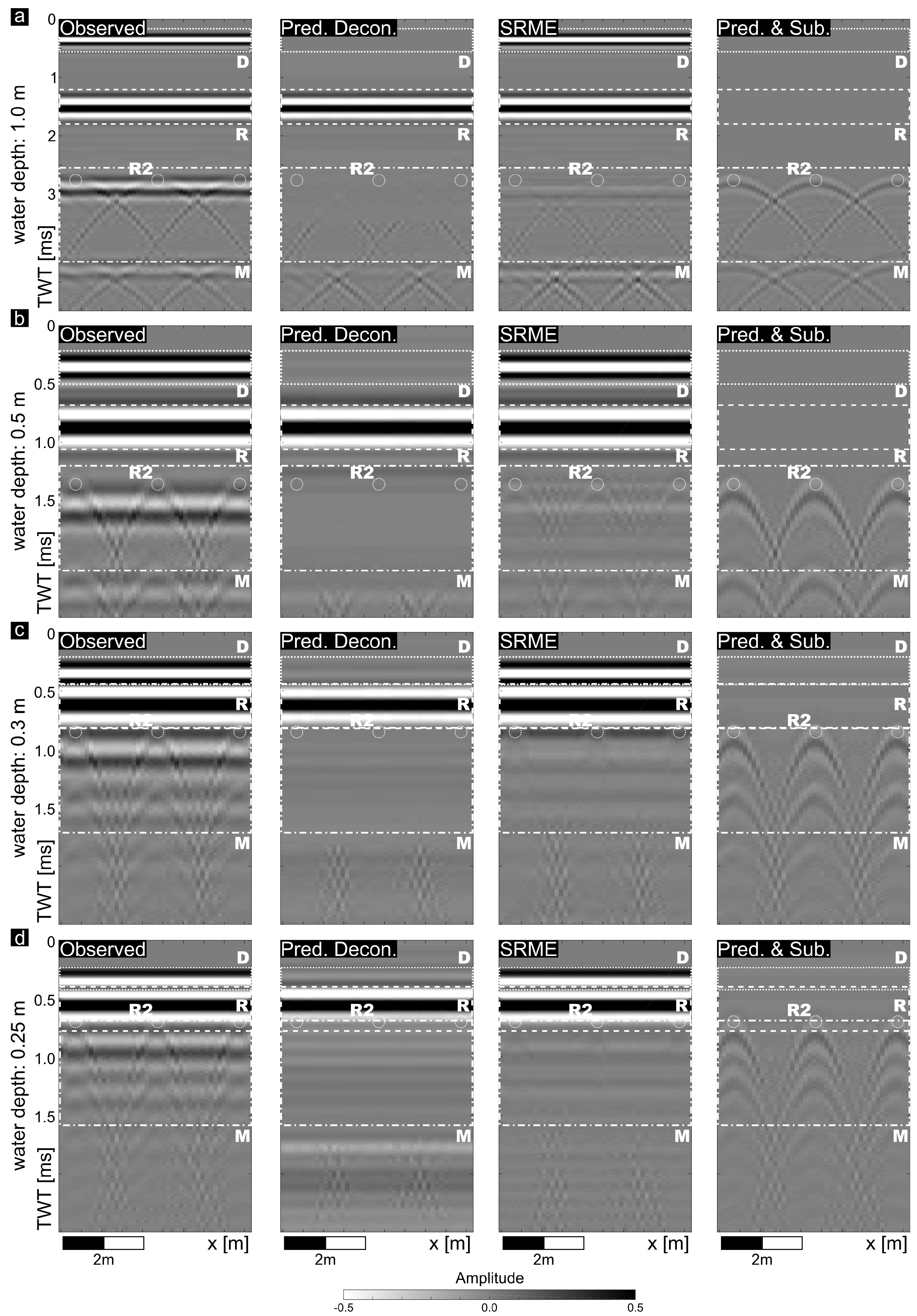
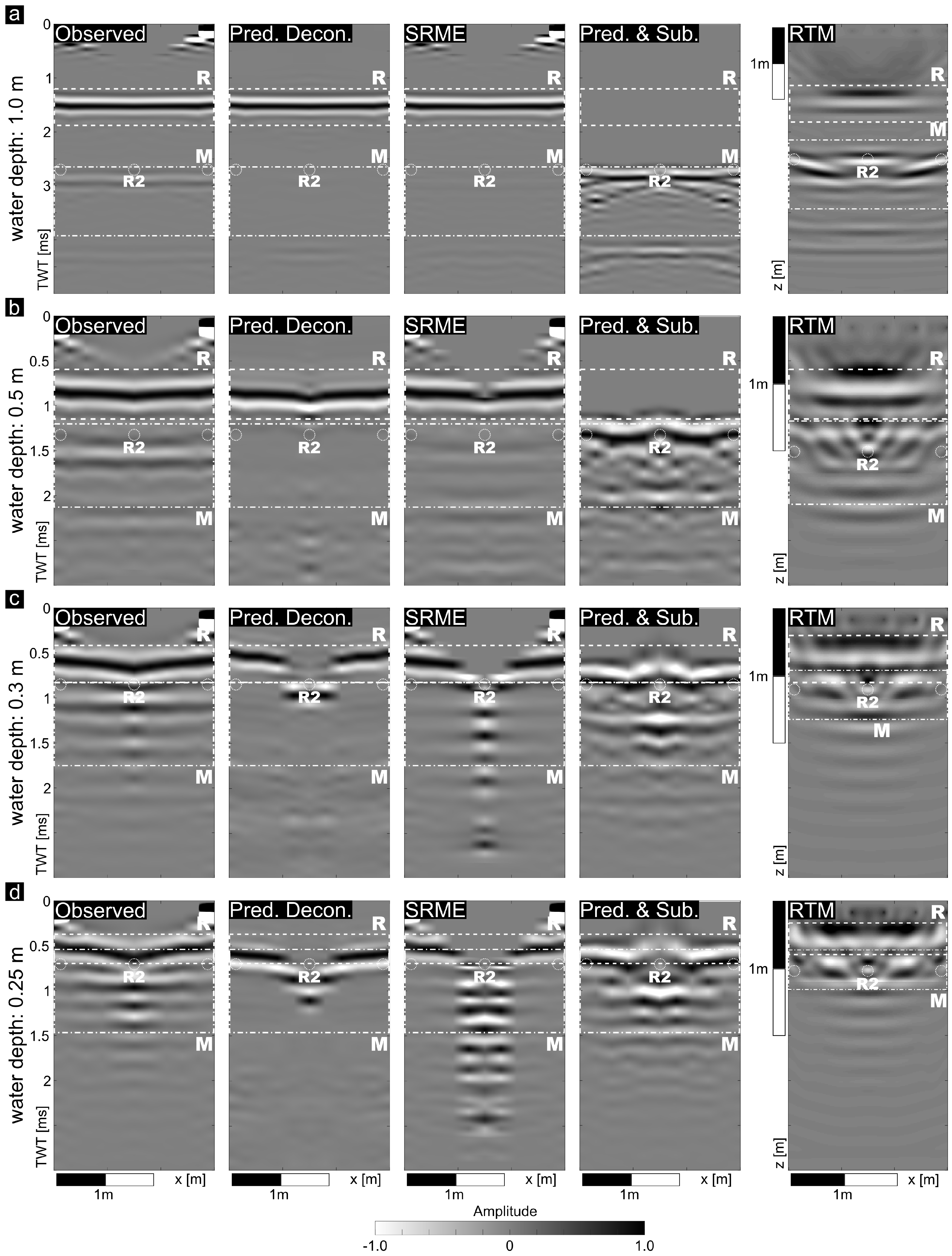
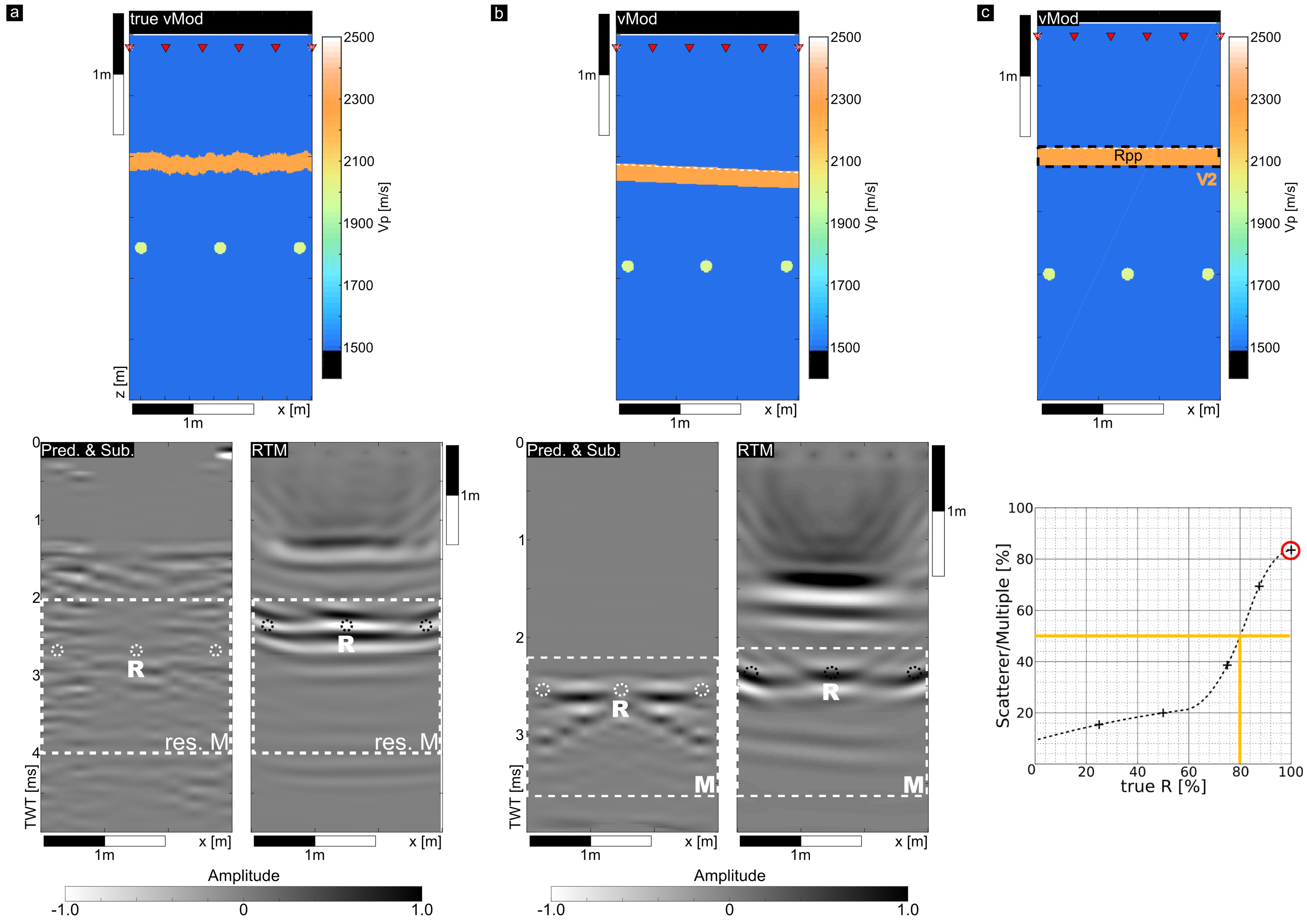
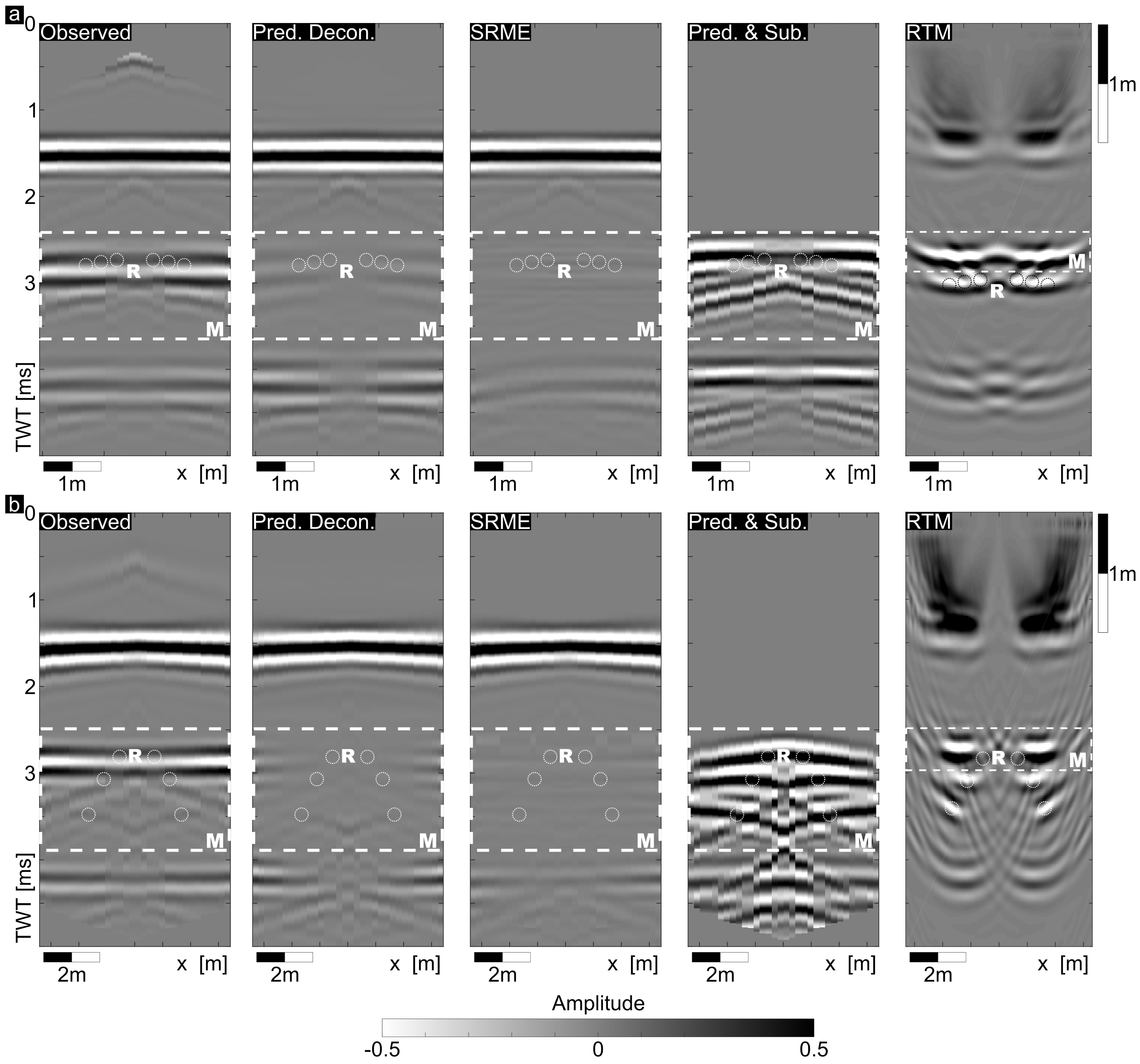
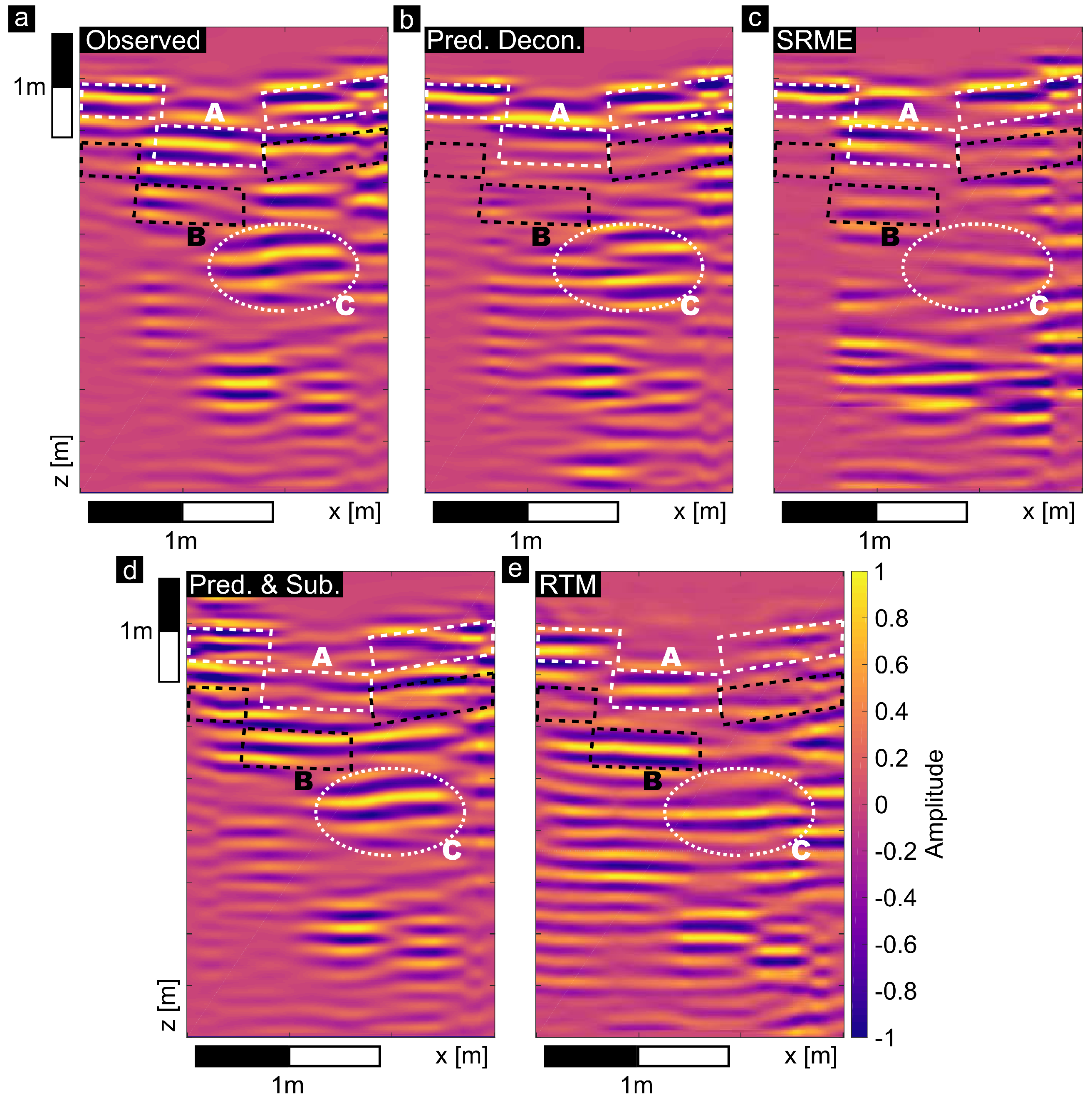
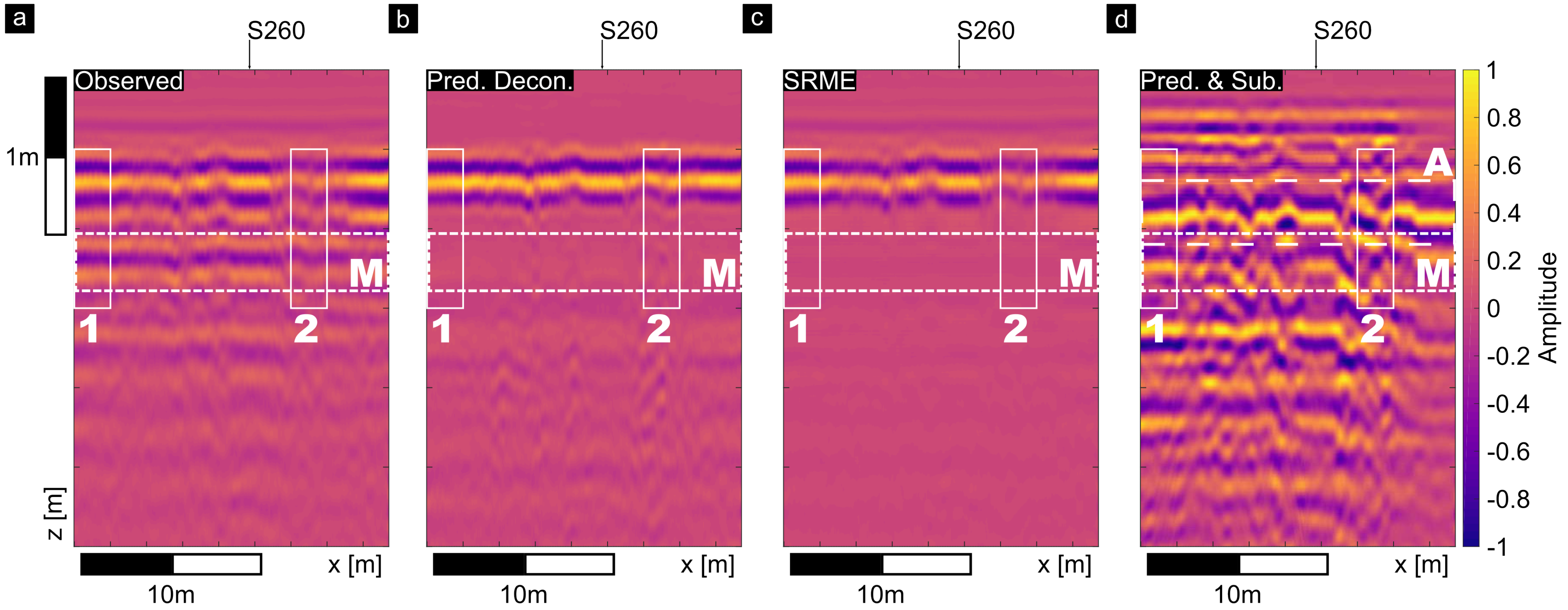
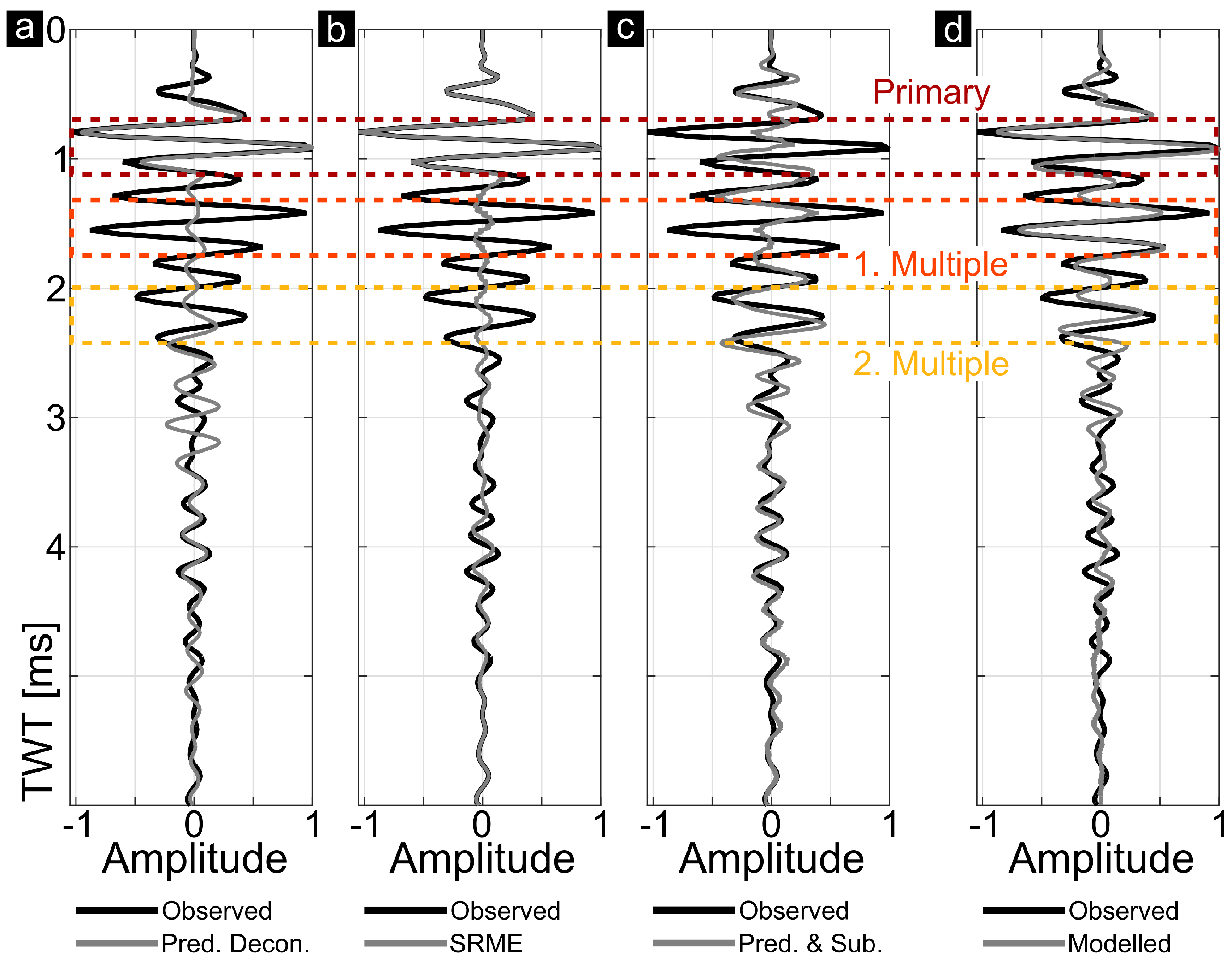
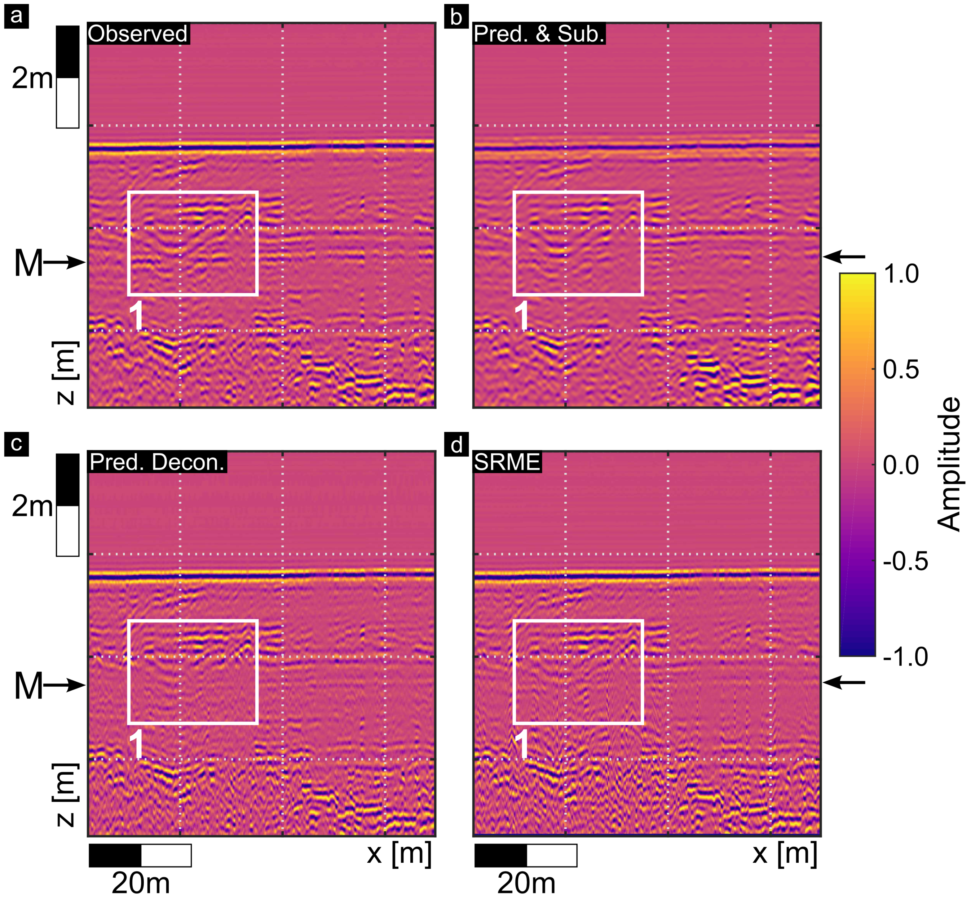
We evaluated two data driven methods using FD modeling of the acoustic wave equation for the attenuation of shallow water-layer multiples for multi- and constant-offset seismic data as recorded for archaeological prospection purposes. In particular, we analyzed the methods with respect to (1) their general applicability, (2) the influence of small uncertainties on the result, (3) traditional methods, and (4) the application to field data sets.

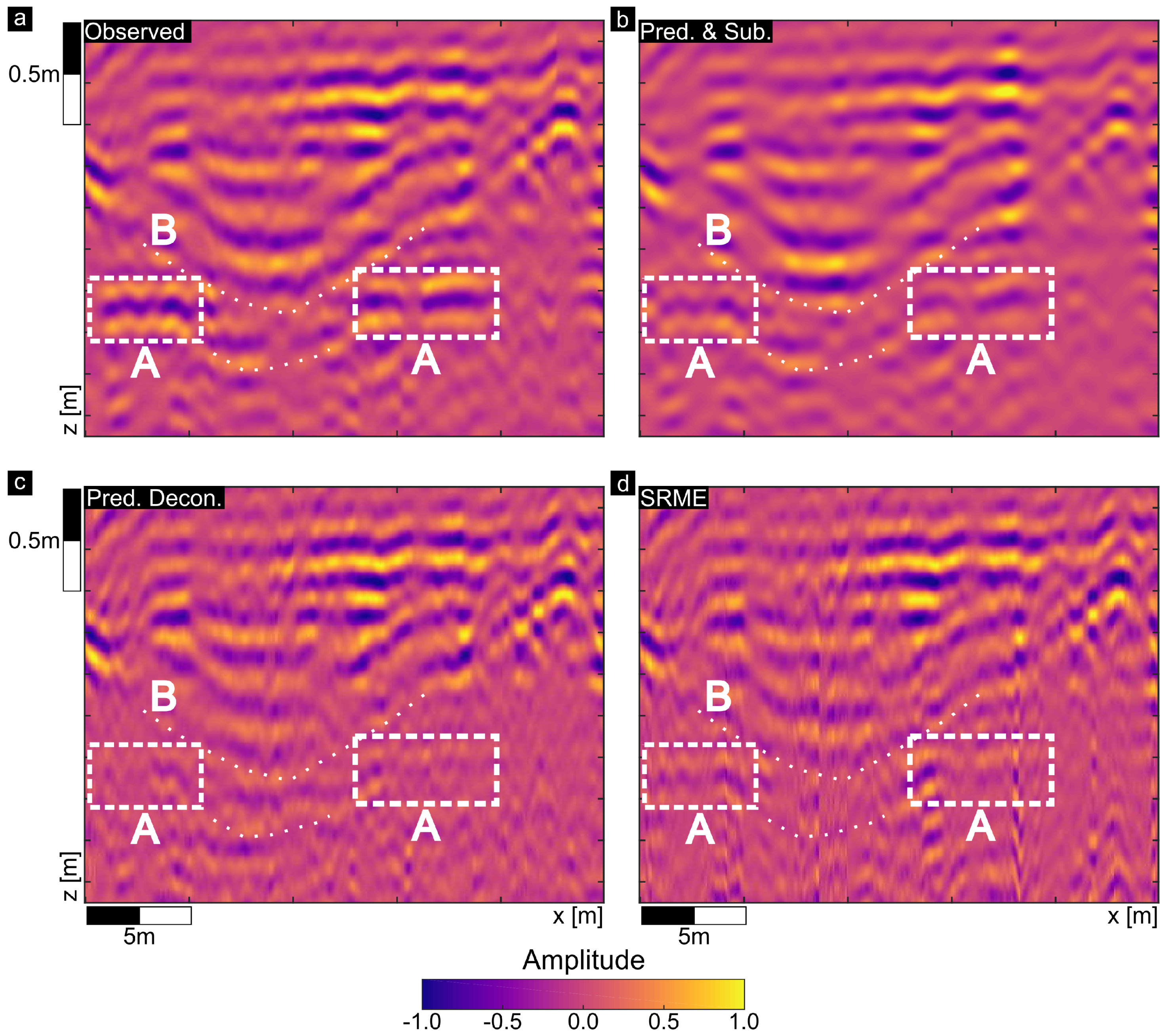
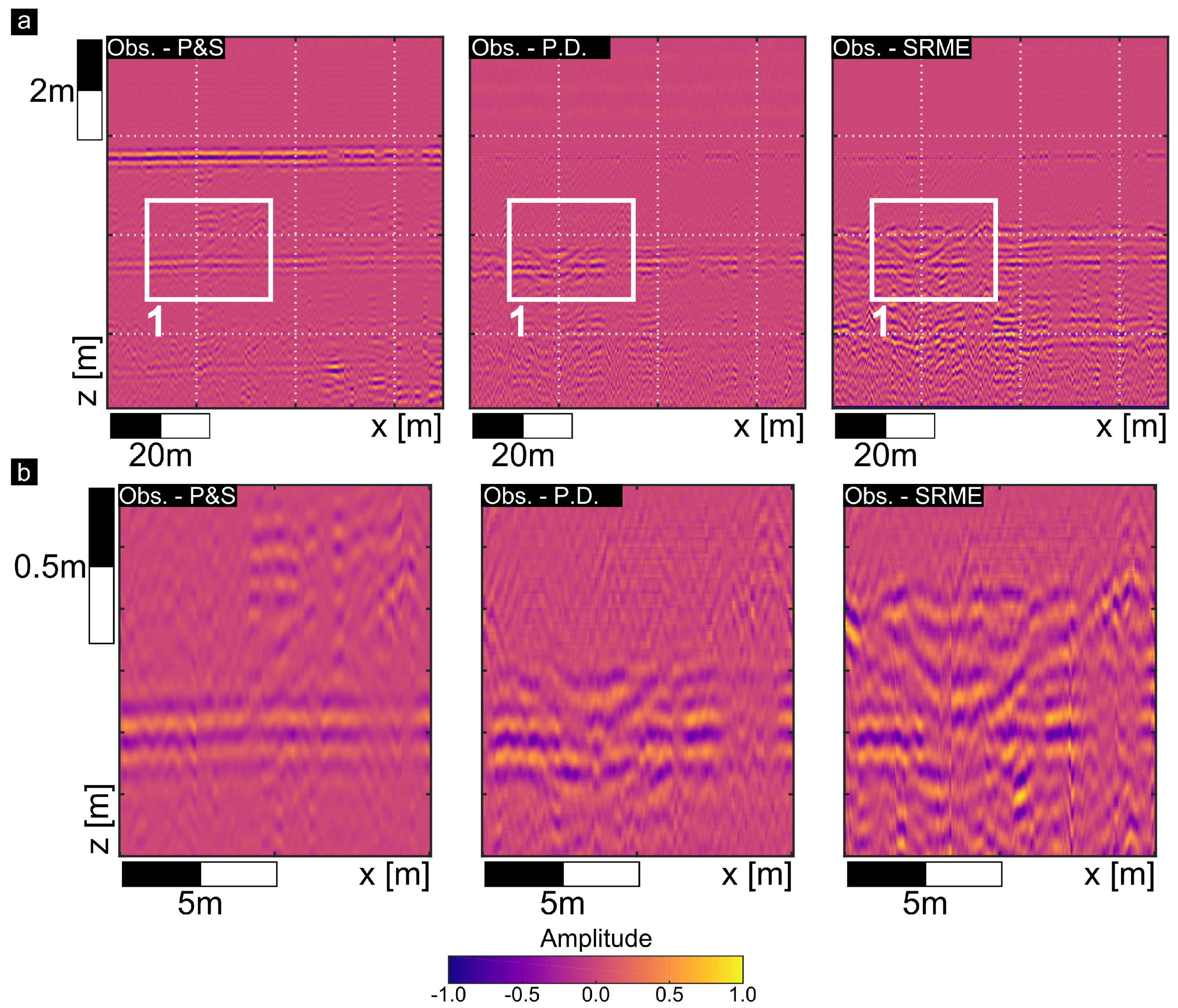
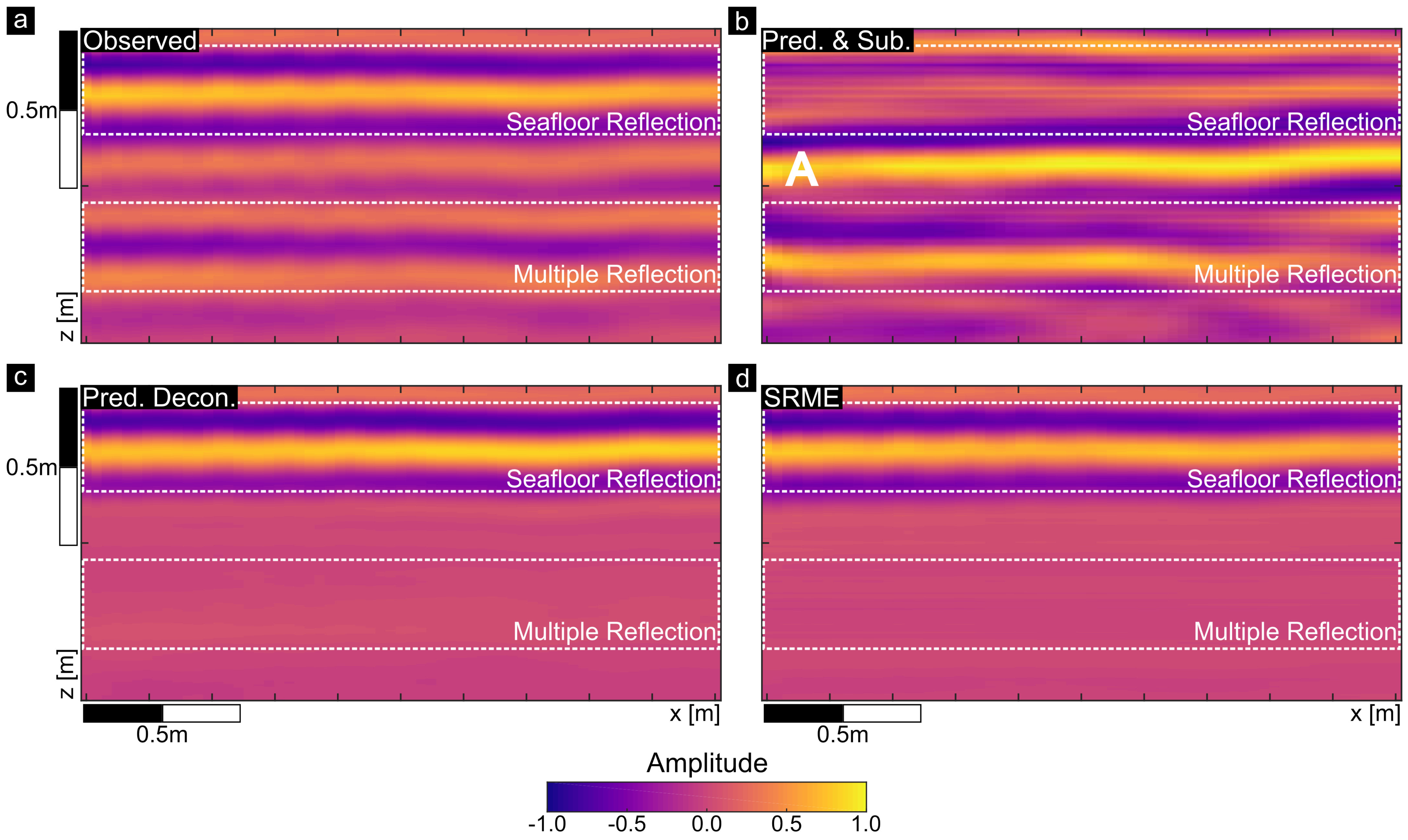
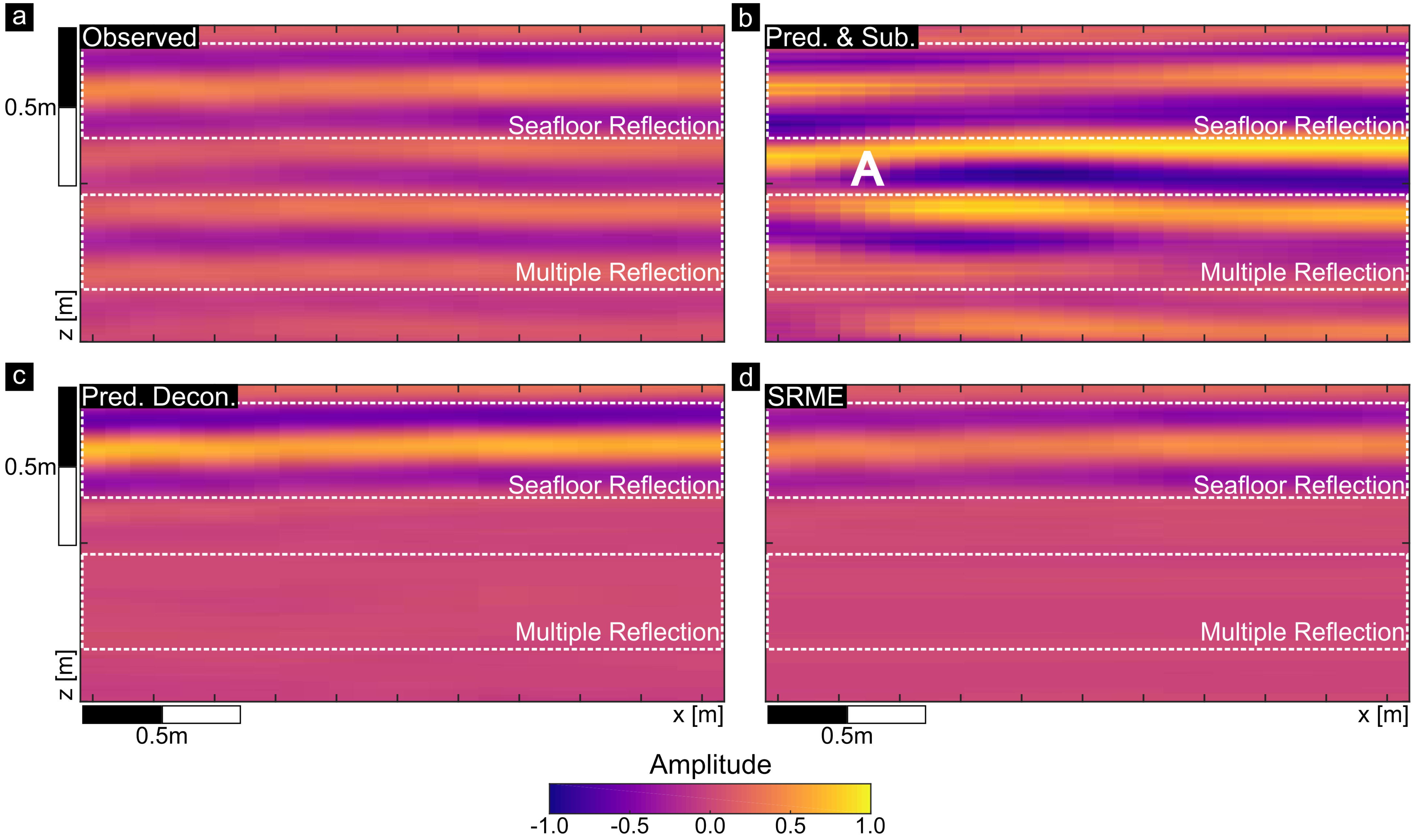
Concerning aspects (1) and (2), both evaluated methods yield satisfactory results concerning the enhancement of primary energy and the attenuation of multiple energy with a reduction of multiple energy of at least 60% and 80%, respectively, for the synthetic test cases by method A and B. Uncertainties in model determination lead to a poorer attenuation of multiple energy, but with an enhancement of primaries of more than 50%, the results are still satisfactory. Furthermore, small differences between the true and the estimated model can be corrected by post-processing of the modeled traces such as time shifts and amplitude adaption. Regarding questions (3) and (4), the evaluated methods A and B achieve comparable results concerning the multiple removal efficiency compared to common methods such as Predictive Deconvolution and SRME, which makes them an attractive tool to be applied in very shallow water demultiple processing. Concerning the enhancement of masked primary reflections, the traditional methods do not perform well as primary signal is attenuated and especially method A is able to achieve better results as the primary is not affected by the processing as it is in Predictive Deconvolution or SRME. This becomes particularly evident in the application to field data examples. The preparation time is approximately equivalent for all methods, but significant differences are given concerning the computational time of the multiple attenuation step. The higher computational costs in the application of method B can be justified by the resulting depth migrated section, which is of further advantage in archaeological investigations.

We conclude that the evaluated approaches, especially the “Prediction and Subtraction” approach, achieve very good multiple attenuation along with an enhancement of primaries when applied to data acquired in very shallow water using either the multi-offset or the constant-offset configuration. Both methods can be transferred to other marine seismic systems and achieve good results in circumstances where the traditional methods fail such as missing near-offsets in shallow water. The field data examples should be emphasized, where tested method A works significantly better than the traditional ones. Although not the ideal conditions are given, the multiples are effectively predicted and attenuated while primary signals are highlighted. In conclusion, this shows that the method is particularly suitable in shallow water applications.

References

1. Von Carnap-Bornheim, C.; Kalmring, S. DFG-Schwerpunktprogramm 1630 “Häfen von der Römischen Kaiserzeit bis zum Mittelalter. Zur Archäologie und Geschichte regionaler und überregionaler Verkehrssysteme”. In Jahresbericht Zentrum für Baltische und Skandinavische Archäologie; Eriksen, B.V., Sonnenschein, I., Eds.; von Carnap-Bornheim, c., Eriksen, B.V.: Schleswig, Germany, 2011; pp. 28–31. [Google Scholar]
2. Passaro, S. Marine electrical resistivity tomography for shipwreck detection in very shallow water: A case study from Agropoli (Salerno, southern Italy). J. Archaeol. Sci. 2010, 37, 1989–1998. [Google Scholar] [CrossRef]
3. Boyce, J.I.; Reinhardt, E.G.; Raban, A.; Pozza, M.R. Marine magnetic survey of a submerged Roman harbour, Caesarea Maritima, Israel. Int. J. Naut. Archaeol. 2004, 33, 122–136. [Google Scholar] [CrossRef]
4. Loke, M.; Lane, J.W., Jr. Inversion of data from electrical resistivity imaging surveys in water-covered areas. Explor. Geophys. 2004, 35, 266–271. [Google Scholar] [CrossRef]
5. Simyrdanis, K.; Papadopoulos, N.; Cantoro, G. Shallow off-Shore archaeological prospection with 3-D electrical resistivity tomography: The case of Olous (Modern Elounda), Greece. Remote Sens. 2016, 8, 897. [Google Scholar] [CrossRef] [Green Version]
6. Fediuk, A.; Wilken, D.; Wunderlich, T.; Rabbel, W.; Seeliger, M.; Laufer, E.; Pirson, F. Marine seismic investigation of the ancient Kane harbour bay, Turkey. Quat. Int. 2019, 511, 43–50. [Google Scholar] [CrossRef]
7. Arcone, S.; Finnegan, D.; Boitnott, G. GPR characterization of a lacustrine UXO site. Geophysics 2010, 75, WA221–WA239. [Google Scholar] [CrossRef]
8. Jol, H.M.; Albrecht, A. Searching for submerged lumber with ground penetrating radar: Rib lake, Wisconsin, USA. In Proceedings of the Tenth International Conference on Grounds Penetrating Radar, Delft, The Netherlands, 21–24 June 2004; pp. 601–604. [Google Scholar]
9. Missiaen, T. The potential of seismic imaging in marine archaeological site investigations. Relicta 2010, 6, 219–236. [Google Scholar]
10. Missiaen, T.; Evangelinos, D.; Claerhout, C.; De Clercq, M.; Pieters, M.; Demerre, I. Archaeological prospection of the nearshore and intertidal area using ultra-high resolution marine acoustic techniques: Results from a test study on the Belgian coast at Ostend-Raversijde. Geoarchaeology 2018, 33, 386–400. [Google Scholar] [CrossRef]
11. Weglein, A.B.; Dragoset, W.H. Multiple Attenuation; Society of Exploration Geophysicists Geophysics Reprint Series: Tulsa, OK, USA, 2005. [Google Scholar]
12. Weglein, A.B.; Hsu, S.Y.; Terenghi, P.; Li, X.; Stolt, R.H. Multiple attenuation: Recent advances and the road ahead (2011). Lead. Edge 2011, 30, 864–875. [Google Scholar] [CrossRef]
13. Weglein, A.B. Multiple attenuation: An overview of recent advances and the road ahead (1999). Lead. Edge 1999, 18, 40–44. [Google Scholar] [CrossRef]
14. Backus, M.M. Water reverberations—Their nature and elimination. Geophysics 1959, 24, 233–261. [Google Scholar] [CrossRef]
15. Goupillaud, P.L. An approach to inverse filtering of near-surface layer effects from seismic records. Geophysics 1961, 26, 754–760. [Google Scholar] [CrossRef]
16. Watson, R. Decomposition and suppression of multiple reflections. Geophysics 1965, 30, 54–71. [Google Scholar] [CrossRef]
17. Anstey, N.; Newman, P. Part II: The sectional retro-correlogram. Geophys. Prospect. 1966, 14, 411–426. [Google Scholar] [CrossRef]
18. Taner, M.T.; O’Doherty, R.F.; Koehler, F. Long period multiple suppression by predictive deconvolution in the x–t domainl 1. Geophys. Prospect. 1995, 43, 433–468. [Google Scholar] [CrossRef]
19. Wiggins, J.W. Attenuation of complex water-bottom multiples by wave-equation-based prediction and subtraction. Geophysics 1988, 53, 1527–1539. [Google Scholar] [CrossRef]
20. Verschuur, D.J.; Berkhout, A.; Wapenaar, C. Adaptive surface-related multiple elimination. Geophysics 1992, 57, 1166–1177. [Google Scholar] [CrossRef]
21. Verschuur, D.; Kabir, M. Comparison of surface-related multiple elimination with Radon multiple elimination. J. Seism. Explor. 1992, 1, 363–377. [Google Scholar]
22. Berkhout, A.; Verschuur, D. Estimation of multiple scattering by iterative inversion, Part I: Theoretical considerations. Geophysics 1997, 62, 1586–1595. [Google Scholar] [CrossRef]
23. Verschuur, D.; Berkhout, A. Estimation of multiple scattering by iterative inversion, Part II: Practical aspects and examples. Geophysics 1997, 62, 1596–1611. [Google Scholar] [CrossRef] [Green Version]
24. Berkhout, A.; Verschuur, D.J. Multiple technology: Part 2, migration of multiple reflections. In SEG Technical Program Expanded Abstracts 1994; Society of Exploration Geophysicists: Tulsa, OK, USA, 1994; pp. 1497–1500. [Google Scholar]
25. Youn, O.K.; Zhou, H.W. Depth imaging with multiples. Geophysics 2001, 66, 246–255. [Google Scholar] [CrossRef]
26. Wilken, D.; Wunderlich, T.; Hollmann, H.; Schwardt, M.; Rabbel, W.; Mohr, C.; Schulte-Kortnack, D.; Nakoinz, O.; Enzmann, J.; Jürgens, F.; et al. Imaging a medieval shipwreck with the new PingPong 3D marine reflection seismic system. Archaeol. Prospect. 2019, 26, 211–223. [Google Scholar] [CrossRef]
27. Bull, J.M.; Gutowski, M.; Dix, J.K.; Henstock, T.J.; Hogarth, P.; Leighton, T.G.; White, P.R. Design of a 3D Chirp sub-bottom imaging system. Mar. Geophys. Res. 2005, 26, 157–169. [Google Scholar] [CrossRef] [Green Version]
28. Plets, R.M.; Dix, J.K.; Adams, J.R.; Bull, J.M.; Henstock, T.J.; Gutowski, M.; Best, A.I. The use of a high-resolution 3D Chirp sub-bottom profiler for the reconstruction of the shallow water archaeological site of the Grace Dieu (1439), River Hamble, UK. J. Archaeol. Sci. 2009, 36, 408–418. [Google Scholar] [CrossRef]
29. Müller, C.; Woelz, S.; Ersoy, Y.; Boyce, J.; Jokisch, T.; Wendt, G.; Rabbel, W. Ultra-high-resolution marine 2D–3D seismic investigation of the Liman Tepe/Karantina Island archaeological site (Urla/Turkey). J. Appl. Geophys. 2009, 68, 124–134. [Google Scholar] [CrossRef] [Green Version]
30. Mueller, C.; Woelz, S.; Kalmring, S. High-Resolution 3 D Marine Seismic Investigation of H edeby Harbour, G ermany. Int. J. Naut. Archaeol. 2013, 42, 326–336. [Google Scholar] [CrossRef]
31. Grøn, O.; Boldreel, L.O.; Cvikel, D.; Kahanov, Y.; Galili, E.; Hermand, J.P.; Nævestad, D.; Reitan, M. Detection and mapping of shipwrecks embedded in sea-floor sediments. J. Archaeol. Sci. Rep. 2015, 4, 242–251. [Google Scholar] [CrossRef]
32. Quinn, R.; Breen, C.; Forsythe, W.; Barton, K.; Rooney, S.; O’Hara, D. Integrated Geophysical Surveys of the French Frigate La Surveillante (1797), Bantry Bay, Co. Cork, Ireland. J. Archaeol. Sci. 2002, 29, 413–422. [Google Scholar] [CrossRef]
33. Nafe, J.E.; Drake, C.L. Physical Properties of Marine Sediments; Technical Report; Lamont Geological Observatory Palisadesny: New York, NY, USA, 1961. [Google Scholar]
34. Richardson, M.; Briggs, K. On the Use of Acoustic Impedance Values to Determine Sediment Properties; Technical Report; Naval Research Lab Stennis Space Center MS: Arlington, VA, USA, 1993. [Google Scholar]
35. El Allouche, N.; Drijkoningen, G.G.; Versteeg, W.; Simons, D.G. Studying converted waves in shallow marine environment. J. Acoust. Soc. Am. 2008, 123, 3597. [Google Scholar]
36. Müller, G. Theory of Elastic Waves; Deutsches GeoForschungsZentrum GFZ: Potsdam, Germany, 2007. [Google Scholar]
37. Claerbout, J.F. Toward a unified theory of reflector mapping. Geophysics 1971, 36, 467–481. [Google Scholar] [CrossRef]
38. Wapenaar, K.; van der Neut, J.; Slob, E. Why multiples do not contribute to deconvolution imaging. In Proceedings of the 79th EAGE Conference and Exhibition 2017, European Association of Geoscientists & Engineers, Paris, France, 12–15 June 2017; Volume 2017, pp. 1–5. [Google Scholar]
39. Poole, T.L.; Curtis, A.; Robertsson, J.O.; van Manen, D.J. Deconvolution imaging conditions and cross-talk suppression. Geophysics 2010, 75, W1–W12. [Google Scholar] [CrossRef] [Green Version]
40. Xiao, C.; Bancroft, J.; Brown, R.; Cao, Z. Multiple suppression: A literature review. CREWES Annu. Rep. 2003, 15, 1–17. [Google Scholar]
41. De Oliveira, A.G.; Gomes, E.D.N.S. Determination of an optimal processing flow for the suppression of free-surface multiples in real 2d marine data. Rev. Bras. Geofísica 2013, 31, 137–149. [Google Scholar] [CrossRef]
42. Verschuur, D.J. Seismic Multiple Removal Techniques: Past, Present and Future; EAGE Publications: Houten, The Netherlands, 2013. [Google Scholar]
43. Hadler, H.; Wilken, D.; Wunderlich, T.; Fediuk, A.; Fischer, P.; Schwardt, M.; Willershäuser, T.; Rabbel, W.; Vött, A. 16 Drowned by the Grote Mandrenke in 1362. In Waddenland Outstanding; Amsterdam University Press: Amsterdam, The Netherlands, 2018; pp. 239–252. [Google Scholar]
44. Milkereit, B.; Spencer, C. Noise suppression and coherency enhancement of seismic data. In Statistical Application in the Earth Sciences; Geological Survey of Canada: Ottawa, ON, Canada, 1989; pp. 243–248. [Google Scholar]
45. Stolt, R.H. Migration by Fourier transform. Geophysics 1978, 43, 23–48. [Google Scholar] [CrossRef]
46. Hung, B.; Yang, K.; Zhou, J.; Guo, Y.; Xia, Q.L. Surface multiple attenuation in seabeach-shallow water, case study on data from the Bohai Sea. In SEG Technical Program Expanded Abstracts 2010; Society of Exploration Geophysicists: Tulsa, OK, USA, 2010; pp. 3431–3435. [Google Scholar]
47. de Oliveira, A.G.; Gomes, E.D.N.S. Offshore east coast: Model-based water-layer demultiple breathes new life into old data. CSEG Rec. 2014, 39, 46–50. [Google Scholar]
48. Berkhout, A. Utilization of multiple scattering: The next big step forward in seismic imaging. Geophys. Prospect. 2017, 65, 106–145. [Google Scholar] [CrossRef] [Green Version]
49. Davydenko, M.; Verschuur, D. Full-wavefield migration: Using surface and internal multiples in imaging. Geophys. Prospect. 2017, 65, 7–21. [Google Scholar] [CrossRef]
50. Komatitsch, D.; Martin, R. An unsplit convolutional perfectly matched layer improved at grazing incidence for the seismic wave equation. Geophysics 2007, 72, SM155–SM167. [Google Scholar] [CrossRef]
51. Groos, L. 2D Full Waveform Inversion of Shallow Seismic Rayleigh Waves. Ph.D. Thesis, Karlsruhe Institute of Technology, Karlsruhe, Germany, 2013. [Google Scholar]
52. Groos, L.; Schäfer, M.; Forbriger, T.; Bohlen, T. The role of attenuation in 2D full-waveform inversion of shallow-seismic body and Rayleigh waves. Geophysics 2014, 79, R247–R261. [Google Scholar] [CrossRef]
53. Fuchs, K.; Müller, G. Computation of synthetic seismograms with the reflectivity method and comparison with observations. Geophys. J. Int. 1971, 23, 417–433. [Google Scholar]
Figure 1. Schematic drawings (left) and photographs (right) of the measuring system setup for (a) PingPong configuration and for (b) constant-offset configuration. The direction of motion in the drawings equals that in the photographs and is indicated by an arrow and circle for the direction out of the image plane. Adapted from [26].
Remotesensing 13 01871 g001
Figure 2. Illustration of the processing steps applied in the tested multiple suppression approaches. Panel (a) shows the basic processing steps of the “Prediction and Subtraction” approach for a multi-offset example. Panel (b) illustrates of the processing steps applied in the “RTM-Deco” approach for a multi-offset example (own configuration).
Remotesensing 13 01871 g002
Figure 3. Schematic representation of the velocity model (a) and exemplary illustration of the absorbing frame (b) for FD modeling of the acoustic wave equation with the PingPong configuration. White asterisks show the source positions, red triangles the receiver positions. The water surface and the water bottom are marked by a white solid and dashed line, respectively. A white dotted line separates the inner model from the absorbing frame. In the velocity model (a), the reflection coefficient at the seafloor is represented by a small lamella of higher velocity (orange) and green circles are scattering objects with velocity v 3 . In panel (b), in the inner model the damping factor σ is defined by Equation (A3), in the outer part by Equation (A8).
Remotesensing 13 01871 g003
Figure 4. Results of multiple attenuation for a synthetic constant-offset section for water depth of 1.0 m (a), 0.5 m (b), 0.3 m (c), and 0.25 m (d). The direct wave (D), the water bottom reflection (R), and the water-layer multiple (M) are marked by white boxes. The positions of the scattering objects are marked by white circles (R2). The results of each applied attenuation approach as well as the original synthetic data are shown for each water depth.
Remotesensing 13 01871 g004
Figure 5. Results of multiple attenuation for a synthetic multi-offset section for water depth of 1.0 m (a), 0.5 m (b), 0.3 m (c), and 0.25 m (d). The water bottom reflection (R) and the water-layer multiple (M) are marked by white boxes. The positions of the scattering objects are marked by white circles (R2). The results of each applied attenuation approach as well as the original synthetic data are shown for each water depth.
Remotesensing 13 01871 g005
Figure 6. Velocity models and results for methods A and B for small scale variations in the water depth (a), a dipping water bottom (b) and incorrect estimation of the reflection coefficient (c). The amount of multiple energy removed for the estimated percentage of true reflectivity is shown in bottom panel (c).
Remotesensing 13 01871 g006
Figure 7. Setup, projection to the x-plane, and velocity models for both the 3D-Chirp (left) and SEAMAP-3D (right) systems. The 3D setup of both systems (a) is projected to the x-plane with all source-receiver offsets (b). Velocity models including scattering objects in a depth equaling the travel time of the first bottom multiple are shown in panel (c).
Remotesensing 13 01871 g007
Figure 8. Seismic sections for the synthetic test cases for both the 3D-Chirp (a) and SEAMAP-3D (b) configurations. The results of the applied multiple attenuation methods are displayed. Except for the RTM sections, all data is NMO corrected with 1500 m/s.
Remotesensing 13 01871 g008
Figure 9. Multi-offset section of field data set 1 from Puck, Poland. The original data (a) and results of all four multiple attenuation approaches are shown (be). The water bottom reflection (A) and the first water-layer multiple (B) are highlighted. C shows a reflection that is enhanced by methods A and B.
Remotesensing 13 01871 g009
Figure 10. Constant-offset section of field data set 1 from Puck, Poland. The original data is shown in panel (a) and results of the multiple attenuation approaches are shown in panels (bd). The extracted multi-offset section S260 (Figure 9) is highlighted by a black arrow. The white boxes 1 and 2 mark details shown in Figure A2 and Figure A3. In the result of the Prediction and Subtraction approach an enhanced reflection is highlighted by a white box with a dashed line (A).
Remotesensing 13 01871 g010
Figure 11. Comparison of the multiple attenuation methods for one exemplary trace of shot 260 of the constant-offset section. The observed data is shown as black trace in all panels, the traces of the particular method are shown in gray. In panel (a) the observed data is compared to the result of Predictive Deconvolution, in panel (b) to the result of SRME, and in panel (c) to the result of method A. In panel (d) a comparison between the observed data and the forward modeled data is shown. The primary reflection is marked in red, the first and second multiple are highlighted in orange and yellow, respectively.
Remotesensing 13 01871 g011
Figure 12. Results of the application of the multiple attenuation methods to field data set 2, (a) constant-offset section acquired in the German North Sea. The observed data is shown in panel a and the results of the Prediction and Subtraction approach is shown in panel (b). For comparison the results of the multiple attenuation with Predictive Deconvolution (c) and SRME (d) are shown. The (attenuated) first water bottom multiple is marked by an arrow. The white box (1) marks details shown in Figure 13.
Remotesensing 13 01871 g012
Figure 13. Detail 1 of the constant-offset section of field data set 2. The observed data (a) and results of three multiple attenuation approaches (bd) are compared. The first water-layer multiple is highlighted with white boxes (A). The enhanced reflector of is marked by a white dotted line (B).
Remotesensing 13 01871 g013
Figure 14. Differences between the observed data and the results of each multiple attenuation method for the whole profile (a) and detail 1 (b), which is highlighted by the white box (1) in a.
Remotesensing 13 01871 g014