
One-Class Classification of Natural Vegetation Using Remote Sensing: A Review

Place du Recteur Henri Le Moal, LETG UMR 6554 CNRS, University of Rennes, 35000 Rennes, France
*
Author to whom correspondence should be addressed.
Remote Sens. 2021, 13(10), 1892; https://0-doi-org.brum.beds.ac.uk/10.3390/rs13101892
Submission received: 29 March 2021
/
Revised: 4 May 2021
/
Accepted: 10 May 2021
/
Published: 12 May 2021
(This article belongs to the Special Issue Remote Sensing Applications in Vegetation Classification)
Abstract
:Advances in remote sensing (RS) technology in recent years have increased the interest in including RS data into one-class classifiers (OCCs). However, this integration is complex given the interdisciplinary issues involved. In this context, this review highlights the advances and current challenges in integrating RS data into OCCs to map vegetation classes. A systematic review was performed for the period 2013–2020. A total of 136 articles were analyzed based on 11 topics and 30 attributes that address the ecological issues, properties of RS data, and the tools and parameters used to classify natural vegetation. The results highlight several advances in the use of RS data in OCCs: (i) mapping of potential and actual vegetation areas, (ii) long-term monitoring of vegetation classes, (iii) generation of multiple ecological variables, (iv) availability of open-source data, (v) reduction in plotting effort, and (vi) quantification of over-detection. Recommendations related to interdisciplinary issues were also suggested: (i) increasing the visibility and use of available RS variables, (ii) following good classification practices, (iii) bridging the gap between spatial resolution and site extent, and (iv) classifying plant communities.
1. Introduction
Mapping and monitoring of natural vegetation classes is essential to conserve and restore biodiversity [1]. However, classification of natural vegetation is challenging given their diversity and dynamics, but also the low quantity of available reference plots [2]. To address this issue, the ecology community used one-class classifiers (OCCs) since the 1980s to map animal and plant species separately [3]. OCCs use few reference plots, which reduced the sampling effort compared to multi-class classifiers [4] such as MaxLike or traditional multi-class support vector machine (SVM). In other words, OCCs enable mapping one class of vegetation without knowing the other vegetation present in the landscape [5]. OCCs require only reference plots related to the class of interest since they do not require absence plots [6]. However, their use remains complex, which implies the need to follow good configuration practices [7] and to interpret the results by combining statistical, spatial, and expert-based indices [8]. Notably, the performance of OCCs is highly sensitive to classifier parametrization (e.g., fitting, thresholding, variable selection) [9,10,11], the quality of the predictive variables used [12], and the reference data [13]. Moreover, assessing the accuracy of OCCs remains challenging without absence data [14].
Although OCCs have been widely used to map natural vegetation in the past decade [4], they usually include only broad-scale bioclimatic variables mainly derived from field plots, which limits their performance [15]. This results in the following challenges: (i) Improving spatial resolution to identify small patches of vegetation [16]; (ii) improving classifier performance by including other variables such as disturbances, or light availability [15]; (iii) improving the spatio-temporal transferability of OCCs [17]; (iv) assessing the impact of global changes on plant community distribution [18]; (v) monitoring changes in biodiversity [19]. In this context, integrating remote sensing (RS) data, which have the advantage of coming from long-term standardized and spatialized observations of the Earth [20], are a growing interest [21]. Paradoxically, although early studies highlighted the ability of RS data in OCCs to increase the accuracy of vegetation classification [22], they remain rarely used [23].
Similarly, in recent years the RS community emphasized the ability to integrate RS data into OCCs to map vegetation [24]. In particular, the new Sentinel satellite time-series or unmanned aerial vehicle (UAV) data offer the opportunity to characterize vegetation classes at unprecedented spatio-temporal scales. Subsequently, combining data from different types of sensors, such as optical and synthetic-aperture radar (SAR), improves classification accuracy [25]. In addition, a wide variety of essential climate and biodiversity variables are now derived from RS data to describe the full range of ecological processes and cover the entire globe, and they are freely available [26]. In this perspective, correspondences between essential climate and biodiversity variables, which are globally recognized indicators for monitoring biodiversity and climate, and RS variables have been established [27].
Integrating RS data into OCCs to map natural vegetation is therefore a multidisciplinary issue: (i) the RS community highlights the emergence of new sensors and new variables derived from the RS data; (ii) the ecological community is interested in the potential of RS data to improving monitoring of vegetation classes but stresses the need to understand clearly how each classifier works. In this context, the objectives of this study are: (i) to review the recent state-of-the-art on the use of remote sensing data for one-class classification of natural vegetation at three hierarchical levels (land cover, plant community, and plant species classes); (ii) to review the state-of-the-art on the tools and parameters used to apply OCCs; and (iii) to highlight the advances achieved in classification of natural vegetation using OCCs, the challenges to be addressed, and further research to be conducted. For this purpose, a systematic review was performed for the period 2013–2020.
2. Literature Search and Review
The literature search was based on expert definition of 79 keywords that were classified into three topics: RS, OCCs, and natural vegetation. Full forms of abbreviations are provided Table S1. The keywords of each topic were combined using the Boolean string “AND” (Table 1) to perform a literature search on the institute for scientific information (ISI) Web of Science (WOS) and Scopus. The literature search extended over 8 years from 2013, when the practical guide to MaxEnt was published [7]. As a result, 1889 and 2082 references that contained the predefined key words either in the title, abstract or key word fields were automatically identified using the search tools available in WOS and Scopus, respectively (Figure 1).
Articles that addressed classification of terrestrial vegetation using airborne or spaceborne RS data were selected. Conversely, articles that focused specifically on fauna, marine ecosystems, virtual species, pathogens, urban habitats, environmental disturbances (e.g., droughts, fires, landslides)—as result of classification—and field RS, as well as duplicates between WOS and Scopus, were excluded, which left 136 articles for the literature review (Table S2). Each selected article was manually reviewed according to an assessment grid with 11 topics and 30 attributes related to the material and classification method used, and each attribute was characterized by one or more categories (Table 2). In addition, the proportion of each attribute category in each of the 11 topics was analyzed and compared to the literature recommendations.
3. A Wide Range of RS Data for Multiple Ecological Considerations
Recent technological advances and current spatial missions provide a large amount of remote sensing data for monitoring vegetation classes. The wide range of available sensors (multispectral; hyperspectral; SAR; LiDAR) and platforms (unmanned airborne; manned airborne; satellite) types provide long-term observation of the Earth and bridge the gap between spatial and temporal resolution. In particular, the emergence of open-access databases of environmental variables (climate; soil; topography; vegetation; categorical; disturbance) with global coverage derived from RS data could improve the classification of natural vegetation. Potential and actual distribution of vegetation classes could be mapped at multiple spatio-temporal scales and hierarchical levels (land cover; plant community; plant species).
3.1. Identifying Potential Restoration or Invasion Areas
Traditionally, OCCs based only on topo-climatic variables were used to map the potential area of vegetation. The addition of RS spectral variables enables OCCs to map not only actual vegetation extent [28] but also potential restoration or invasion areas [29]. However, the literature review indicates that while most studies classified only the potential or actual vegetation area, these two components were rarely considered together (Table 3). Generally, many studies that classified potential vegetation area (n = 27) used spectral variables as an indirect descriptor. For examples, photosynthetic activity derived from a SPOT-NDVI time series at a 1 km spatial resolution was used to classify the potential extent of tree species [30], and LiDAR-derived light availability was used to classify the potential extent of understory species [31]. Interestingly, several studies classified the potential area of vegetation using topo-climatic variables and then classified the actual vegetation area using vegetation variables [5,32,33].
3.2. From Plant Species to Land Cover
Vegetation classes can be mapped at different hierarchical levels, ranging from plant species to land use/land cover (LULC). The literature review highlights that most studies classified vegetation at the species level, especially for invasive species [34,35,36] or endangered species [37,38,39], while the coarser LULC level and the finer plant-community level were studied less (Table 4). At the LULC level, most studies investigated the influence of classifier parameters on map accuracy, since over-detection of LULC classes can be detected clearly from visual interpretation of images [40,41,42,43,44]. Others studies focused on wetland inventories [45,46,47] or farming areas [48]. At the plant-community level, the typology studied ranged from plant associations [49,50] to natural habitats [5,51,52,53]. Interestingly, Bradter et al. [49] and Fenske et al. [50] indicated that increasing the vegetation hierarchical level (i.e., from habitat to plant association or species) decreases OCC accuracy, while Suárez-Seoane et al. [54] demonstrated the opposite. In addition, Suárez-Seoane et al. [54] and Connor et al. [55] showed that vegetation classes with a narrow ecological niche had higher classification accuracy than that with a wider niche. To improve the classification accuracy of plant communities, Tang et al. [56] developed an approach that groups species into spectrally discriminating phenological groups based on a k-means classification applied to PCA axes of MODIS spectral variables. However, using RS data at moderate spatial resolution to map plant species raises the issue of the influence of the spatial resolution of RS data on vegetation detection [57].
3.3. Site Extent and Spatial Scale
The size of the study site is crucial for OCCs: the larger the size and variety of environments considered, the more transferable the classification will be to other parts of the world [17]. Furthermore, the use of RS spectral variables in OCCs hinders the transfer of classifications to other study sites given the phenological shifts that occur between sites and years [53]. The literature review supports that, as the size of the site increases, the scale of analysis decreases. For examples, (i) peatlands were classified at a metric resolution on a site of a few ha using QuickBird and WorldView-3 satellite images [47]; (ii) Kim et al. [58] and Doninck et al. [59] classified plant species using 30 m Landsat images across South Korea and the Amazon, respectively; and (iii) biomes were mapped over the entire earth using kilometric-resolution MODIS products [60].
3.4. Long- or Short-Term Vegetation Monitoring
RS data, which provide standardized spatio-temporal measurements, have great potential for monitoring of vegetation [61], particularly in the long term [24]. Nonetheless, the literature review indicates that temporal monitoring of vegetation was rarely addressed (n = 14) and that change was often detected by comparing classifications date-by-date, which sums the errors from each classification [62]. Half of the studies monitored vegetation classes over the long term (~40 years) at decadal intervals using high spatial resolution Landsat satellite imagery [48,63,64]. Others performed mid-term monitoring (~15 years) at annual intervals using MODIS moderate spatial resolution satellite imagery [39,65]. Two studies performed very-long-term (~90 years) monitoring at 20-year intervals using LULC variables derived from historical aerial photographs [66,67], and only one study performed short-term (8 years) monitoring using two very high spatial resolution satellite images [47]. Regarding forecasting, four studies used long-term classification (~100 years) that combined LULC and climate variables simulated under different scenarios [66,68,69,70].
3.5. The Importance of Spatio-Temporal Resolutions
The RS data used in OCCs should remain consistent with the spatio-temporal scales of vegetation [29]. However, given the specific limitations of RS sensors (e.g., high spatial but low temporal resolution vs. low spatial but high temporal resolution), scaling issues may arise in the ecological interpretation of vegetation maps. Temporal resolution is also critical: single-date RS data may have been acquired at a time that does not represent ecosystem functioning [61]. In addition, classification accuracy increases as the number of acquisitions used increases [29]. The new Sentinel data have addressed these technical limitations by combining high spatial resolution (10 m) with high acquisition frequency (7 days), which helps characterize and monitor vegetation classes at new spatio-temporal scales [24].
The literature review confirms issues caused by using RS data at inadequate spatial and/or temporal resolutions to map vegetation classes. Most studies (91%) that use RS data with moderate-to-low spatial resolution classify plant species. Interestingly, Connor et al. [55] found that OCC accuracy decreased as the spatial resolution of an RS-derived DTM decreased, and recommended selecting RS data with a spatial resolution similar to that used to collect the reference plots.
The review shows that vegetation classes were characterized mostly from single-date and, to a lesser extent, multi-date or time-series RS data (Table 5). Although Sentinel-1 and Sentinel-2 data have been freely available since 2014 and 2016, respectively, their use for mapping vegetation in OCCs remains low (n = 6). Indeed, most studies used multi temporal Sentinel-2 images [45,71,72,73,74] whereas one study used Sentinel-1 images [75].
Recently, vegetation variables at centimetric resolution derived from UAV data are increasingly used in OCCs. For examples, (i) Multispectral sensors on UAVs can map invasive species [76] or small patches of plant communities [77]; and (ii) point clouds generated from stereoscopic UAV data can characterize the vertical structure of vegetation at unprecedented spatial resolution [78]. Interestingly, Kattenborn et al. [75] demonstrated that UAV data can be an effective alternative to field data for fitting and validating OCCs based on satellite imagery. However, UAVs can currently cover only a few ha (1 ha equals to 10,000 square meters), which reduces their usefulness for local monitoring.
3.6. Underused RS-Based Environmental Variables
The number of studies that use each type of ecological variable based on RS or field plots is shown in Figure 2. Globally, the results show that vegetation, climate, and topography variables are the most frequently used in OCCs, while soil, geology, and disturbance variables are rarely used. Moreover, vegetation, topography, LULC and disturbance variables are mostly derived from RS data, whereas climate, soil, and geology variables are largely produced from field observations. From recent years, open access and RS-based soil [79], climate [80], or disturbance variables such as snow cover [81] are available and should be used more frequently in OCCs.
The vegetation variable (i.e., spectral values) is used most often (n = 99) and comes exclusively from RS data. Specifically, several studies showed the utility of variables that characterize vegetation phenology derived from multispectral satellite data to map natural vegetation, such as MODIS [82,83], Landsat [54], ASTER [84], RapidEye [51], or hyperspectral airborne data [85]. Although Sentinel-2 data are increasingly relevant for OCCs, their use remained limited to a few acquisitions [45,71,72,73]. Notably, Delalay et al. [74] reported the utility of Sentinel-2 time-series in OCCs for mapping vegetation classes in Nepal. In addition, vegetation variables that characterize the vertical structure and volume of vegetation derived from high and very high spatial resolution LiDAR and SAR data are highly useful for OCCs [24,25]. For examples, Mack and Waske [44] classified LULC using a TerraSAR-X time series; and Kattenborn et al. [75] classified woody species using a combination of Sentinel-1 and -2 data. In practice, few studies used SAR-derived vegetation variables in OCCs to map vegetation, despite the growing interest in Sentinel-1 images. Regarding specific application of LiDAR data, canopy height is the vegetation variable used most often in OCCs [5,86,87]. Wüest et al. [31] recently demonstrated that a light-availability variable derived from a LiDAR point cloud increased the accuracy of OCCs for understory tree species.
Climate variables describe the tolerance of vegetation to water and temperature [4] and were derived mostly from GIS field-based layers (n = 67), such as WorldClim (~1 km resolution) data [88], were also used frequently (n = 89). However, variables for precipitation and temperature derived from multispectral time series, such as land surface temperature products derived from MODIS data at 0.1 degree [89] (and up to 250 m resolution over Europe [90]), or MERRAclim (2.5 arc minutes) [80], are freely available. Deblauwe et al. [91] and Cord et al. [82] revealed that these RS-derived climate variables increased the accuracy of OCCs more than WorldClim data, especially in areas with a low density of weather stations and/or high environmental gradients. MODIS Land Surface Temperature products also include a night temperature component, which is a highly informative variable for the distribution of invasive species [92]. In this context, Lembrechts et al. [93] recommend selecting climate variables derived from RS data rather than using low-resolution WorldClim data systematically.
Topographic variables, which characterize energy and moisture availability [4], are also widely used in OCCs (n = 87), particularly variables derived from RS data (n = 66). The Shuttle Radar Topography Mission DEM provides global coverage at a 90 m spatial resolution and is used in OCCs at continental and regional scales [46], while airborne LiDAR data provide very high spatial resolution topographic variables for OCCs [5,94]. For sites not covered by LiDAR data, but where high spatial resolution is required, the free Global DEM at 30 m spatial resolution generated by stereoscopy of ASTER satellite data is a suitable alternative to improve the spatial scale of OCC maps [65,95,96]. Similarly, DEMs generated at high spatial resolution (12 m) from ALOS PALSAR data were used successfully to map habitat suitability of plant species of the genus Juniperus in Iran [97].
LULC is commonly used in OCCs (n = 41), since it characterizes whether LULC types are suitable (e.g., woods, grassland) or not (e.g., built-up, crop) for the distribution of plant species [4]. Literature review shows that all LULC variables used in OCCs were derived from RS data. For example, the European CORINE Land Cover or USGS National Land Cover Database layers used in OCCs [98,99] were generated at 1:50,000 scale from Landsat satellite images. At finer spatial scales, LULC variables can be derived from very high spatial resolution RS data, such as aerial photographs and LiDAR data [100]. However, Cord et al. [101] highlighted that thematic resolution was more important than spatial resolution. Interestingly, OCC accuracy could be increased by using LULC change variables [26].
Although soil and geological conditions influence the distribution of natural vegetation, these types of variables remain less widely used in OCCs (n = 25 and 7, respectively) due to their partial coverage, spatial scale, and coarse-pixel size. Nonetheless, two studies used high spatial resolution soil-property variables derived from reflectance values of airborne [102] or satellite [103] multispectral sensors. Recently, SoilGrids layers that cover the entire earth at 250 m spatial resolution and characterize soil properties (e.g., pH, texture, carbon) and soil classes (World Reference Base) were derived from MODIS satellite data [79]. Four studies noted the contribution of these SoilGrids variables to OCCs for mapping natural vegetation [99,104,105,106].
RS data are often used to map and monitor disturbances (e.g., floods, snow cover, fires, landslides) [26], mainly fire events derived from high spatial resolution satellite data [39,107] and snow duration derived from MODIS [60] or Landsat [108] images. Surprisingly, these data remain little used (n = 4) as input variables to classify vegetation.
3.7. Combining Variables Improves OCC Performance
In theory, Mod et al. [15] recommended using a set of seven ecological variables in OCCs: temperature, water, nutrients, light, biotic interactions, disturbances, and LULC. In this perspective, Fois et al. [109] advised combining bioclimatic variables with at least two other types of variables. However, the literature review indicates that most studies use fewer than three types of variables (Figure 3). Given the similar spectral responses among plant species, several studies reported a decrease in classification accuracy when variables derived from RS data were used alone [5,106,110,111]. Conversely, many studies have reported not only that adding a spectral variable to environmental variables increases OCC accuracy [82,110,111,112], particularly when classifying climate-unstructured plant species [59], but also that the spectral variable often contributes the most [36,46]. Two other studies reported that adding spectral variables did enhance the spatial scale of the map substantially [54,106]. Only 25 studies used at least four variable types. For example, Mudereri et al. [105] classified the potential area of an invasive plant species in Zimbabwe using a combination of five variable types (i.e., bioclimate, vegetation, topography, soil, and LULC) derived only from RS data.
3.8. Data Quality Influences OCC Performance
The quality of predictive variables and reference data influences OCC performance [5,12,24]. The literature review indicates that variables derived from RS data can be influenced by the specific characteristics of the sensor, environmental conditions, or data processing. For examples, (i) Lopatin et al. [78] showed that shadows in very high spatial resolution images decrease classification accuracy; (ii) Moudrý et al. [12,113] found that variable topographic quality (e.g., spatial resolution, ability to penetrate vegetation cover, parameters for calculating topographic indices) influenced OCC accuracy greatly; (iii) Randin et al. [26] indicated that spectral values of the thermal bands used to generate bioclimatic variables are also influenced by the land-cover; (iv) Cord et al. [101] and Truong et al. [106] stated that the quality of the LULC variable (e.g., spatial resolution, thematic resolution, map reliability) often influences OCC accuracy and suggested replacing LULC categorical variable with continuous spectral variables.
Regarding reference data, their quality is also an issue for OCC performance [54]. Although new reference plots can be collected according to a specific protocol suitable for classifying actual area of vegetation classes at local or regional scales, using field reference databases is inevitable when classifying larger sites and/or performing temporal monitoring. These reference databases are frequently subject to spatial sampling bias, incorrect georeferencing, or incorrect descriptions of vegetation [24,75]. In this sense, Suárez-Seoane et al. [54] highlighted that compiling multiple regional reference databases into a national database is challenging, since the same vegetation patch may be described differently depending on the criteria that each botanist used. Moreover, spatial errors can occur when relating field vegetation plots to the predictor variables, since one pixel may include diversity of vegetation classes [40]. However, the literature review illustrates a few approaches to correct biases in reference data:
- Subsampling: Several authors corrected for spatial sampling bias by subsampling reference data in densely plotted areas [118].
- UAV image analysis: Reference data can be derived automatically from very high spatial resolution UAV images [75]. This approach is interesting since pure pixels can be extracted from reference polygons, and reference data can be collected from sites that are difficult to access in the field.
4. A Wide Range of Tools and Settings for OCCs
4.1. Classifier Selection
The variety of OCCs can be classified into three main groups: regression (e.g., partial least square), machine learning (e.g., generalized linear model, generalized additive model, random forest, MaxEnt), and deep learning (e.g., convolutional neural network). Interestingly, the traditional multi-class SVM classifier can be adapted to one-class by the use of absence points [44]. Overall, Yates et al. [17] indicated that it is challenging to rank the best classifiers, since the results are specific to each study (e.g., vegetation class and hierarchical level, quantity and quality of reference data, environmental variables, fitting and validation methods). Several studies noted that classification accuracy was similar regardless of the machine-learning classifier used [52,97]. In addition, it could be useful to create an ensemble classifier i.e., applying multiple OCC and then combining each classifier’s predictions to highlight the differences and thus the uncertainties [17]. The literature review indicates that most studies used machine-learning, or to a lesser extent, ensemble classifiers, but fewer used regression classifiers (Figure 4). Only one study used an evolutionary classifier [119], which performed worse than a MaxEnt classifier. Three other studies used deep-learning OCC to accurately map vegetation classes [77,120,121].
4.2. Tools and Computer Resources
Previous recommendations addressed the wide use of open-source software [122] and cloud computing [123]. The literature review confirmed that most studies (n = 126) used open-source software to map vegetation class, such as R and its packages “dismo” [124], “ENM eval” [125], “spatialEco” [126], “BIOMOD” [127], and “maxnet” [128]. Conversely, a few studies (n = 29) used commercial software to pre-process RS data, particularly hyperspectral data or those acquired by the UAV platforms. Only five studies used cloud computing to classify the natural vegetation [60,65,74,129,130], such as the commercial platforms Google Earth Engine [131] and Amazon Web Services [132].
4.3. Variable Selection
Variable selection is essential to improving OCC transferability [17] and limiting over-fitting [7], especially when a large number of variables derived from satellite time series are included. According to the ecology community, only RS variables that make ecological sense for the vegetation type classified should be used [28]. Statistical approaches that reduce dimensions should be avoided since they remove the ecological significance of each variable [4]. In 2013, Rocchini [61] observed that some studies do not explicitly state the significance of the RS variables used in OCCs for natural vegetation mapping.
The literature review reveals first that the selection of variables is based mainly on expert-based approaches (n = 71), the existing literature (n = 36), and, to a lesser extent, data mining (n = 29) that consider all possible variables. Then, variable collinearity is addressed mainly by statistical approaches based on internal classifier functions, a correlation statistical index, and dimension reduction, while expert-based approaches—involving the knowledge on the environmental and ecological characteristics of the vegetation classes—are rarely used (Figure 5).
4.4. Background vs. (Pseudo-)Absence Points
Guillera-Arroita et al. [133] noted confusion over the definition and use of the terms “background,” “pseudo-absence,” and “absence” points. Background points are used for “presence-only” classifiers (e.g., MaxEnt, biased-SVM) to describe the landscape and can thus be located close to the field reference data. Absence and pseudo-absence points indicate actual or expected absence, respectively, and are used for “presence/absence” classifiers (e.g., random forest, generalized linear model). The number and location of background points are usually selected arbitrarily [8] and can influence classification accuracy strongly. Therefore, this step should be applied with caution [9]. Spatial bias is inevitably generated by an uneven distribution of field reference data [114]. Several methods have been developed to correct this bias, such as “bias correction” [134], which places less importance on background points far from the densely plotted areas, or “background thickening” [135], which preferentially selects background points located in densely plotted areas. Background points should be selected over the entire landscape, including the immediate surroundings of the occurrence data; if not, classification accuracy may be overestimated [134]. The number of background points selected is set by default to 10,000. This number can be adjusted according to the size of the study site and the spatial resolution of the predictive variables [7].
The literature review highlights that:
- Confusion over the use of background and pseudo-absence points still occurs (Table 6): 42% of studies based on “presence-only” classifiers mentioned the use of pseudo-absence or absence points. Conversely, and to a lesser extent, 7% of the studies based on presence/absence classifiers used background points. This confusion occurred mainly in “ensemble classifiers” that combined presence-only and presence/absence OCC.
- The number of randomly generated background points varied greatly, from 200 points [45] to 50,000 points [115]. Most often (n = 49), the number of background points was unspecified and thus probably defaulted to 10,000. Conversely, many studies explicitly mentioned this default value (n = 26). A few studies used less than 10,000 points (to decrease calculation times [85]) (n = 9) or more than 10,000 (n = 4).
- Spatial bias was rarely assumed when generating background points (n = 10).
- Background points were usually selected over the entire landscape (n = 29), although most studies (n = 51) did not specify this. Seven studies selected background points only in natural areas.
- The selection of background points rarely excluded the areas with field vegetation plots (n = 6).
4.5. Classifier Fitting
Classifier fitting aims to test all the possible configurations (i.e., classification parameters and their related values) to optimize the performance. Several authors recommended that transferability should be given priority over classifier performance during the fitting step [14,118]. The literature review confirms that a large number of studies that classified natural vegetation used the default configuration instead of fitting the classifier (Table 7). Surprisingly, this step was rarely applied in OCCs, particularly with MaxEnt classifier [10] since its predefined settings enable easy running [44]. This lack of classifier fitting may also be motivated by the long calculation times [51] or complexity of some machine-learning classifiers [46]. In details, the primary aim of OCC fitting is to increase accuracy and, to a lesser extent, transferability (Table 7). Results indicated that fitting improved OCC performance [42,136], while others demonstrated that fitting had little influence on it [44,137].
It should be kept in mind that the classifier fitting step is based on accuracy index. The literature review stresses that the F-score was often used as an alternative to the area under the curve (AUC) to increase the classifier performance [47,138], while Akaike’s Information Criterion (AIC) was used to increase the classifier transferability [83,137,139]. Interestingly, West et al. [83] studied the temporal transferability of OCCs and found that a MaxEnt classifier fitted with the reference data acquired in 2007 and had AIC values similar to those of a classifier fitted with reference data acquired six years later.
Several studies have used novel approaches or tools to improve OCC fitting. For example, Piiroinen et al. [87] used a function from the R package “oneClass” that fitted a classifier by thresholding the F-score (a threshold-dependent metric) at different values. Vollering et al. [140] developed a tool to improve the ecological interpretation of OCCs by distinguishing effects of classifier fitting from those of variable transformation. Yu and Kang [141] developed an unsupervised learning approach that accommodates OCC that can be fitted without using absence data.
4.6. Thresholding
Thresholding is an optional step parameter that may affect the accuracy of OCCs [4,11]. For this reason, Merow et al. [7] recommended avoiding thresholding. Thresholding can occur two times in the classification process: (i) during classifier fitting and validation steps, when using a threshold-dependent index (e.g., F-score, Kappa); and (ii) when converting continuous maps to categorical maps (presence/absence). Among many threshold indices (e.g., automatic, expert based), Liu et al. [142] demonstrated in 2013 that the “maximum sensitivity specificity” index was the most effective for OCCs.
The literature review confirmed that thresholding is the parameter that influences the accuracy of OCCs the most [42,73] and that a threshold remains challenging to set [51,53]. Although Chignell et al. [46] noted that a continuous map is more informative than a categorized map for end-users, few of the studies reviewed avoided thresholding (Table 8). Conversely, most studies used a threshold during OCC fitting and validation, and/or map categorization.
Statistical thresholding was used more frequently (n = 76) than expert-based thresholding (n = 20), though the thresholding method was not always specified (n = 7). Cord et al. [82] compared several statistical indicators and confirmed that the “maximum sensitivity specificity” index is the best indicator for OCCs. However, no consensus emerges [53], since the literature review includes a wide variety of statistical indices, such as:
- Maximum F-score [50];
Regarding expert-based thresholding approaches, many authors stated that they inevitably remain subjective [43,87]. For example, a threshold value of zero (i.e., the hyperplane) was used to fit SVM classifiers [137,138], and a threshold of 0.5 was used to categorize maps [139,146]. Studies may benefit from developing a threshold-free approach and using threshold-independent indices combined with continuous maps. In this perspective, Scherrer et al. [11] recently developed an original approach to classify plant communities without thresholding.
4.7. Assessing Classification Accuracy
Traditionally, the quality of OCCs was assessed using statistical indices [4]. However, given sampling biases (e.g., spatial autocorrelation, no absence data), accuracy indices must be interpreted carefully [43] and supplemented with expert-based map validation [8]. To limit statistical bias, classification accuracy should be assessed using reference data that are independent from those used for OCC fitting and spatially uncorrelated [14]. Furthermore, assessment of over-detection by OCCs is biased without absence reference data.
The literature review highlights that classification accuracy was assessed mainly using statistical validation through performance (n = 123) and/or transferability (n = 13) indices. Fernandes et al. [147] reported that the Kappa index is more sensitive to degradation of the quality of reference data than the AUC or TSS. Morales and Fernández [73] suggested not placing all confidence in statistical indices of classifier quality (e.g., AUC, AIC, TSS), but rather in conventional Kappa or global accuracy indices derived from independent reference datasets.
Unlike statistical validation, spatial validation was rarely performed, either by expert-based (i.e., visual) map analysis (n = 8) or by interpreting spatial uncertainty indices (n = 4). Several original approaches deserve to be pointed out: (i) Stenzel et al. [53] estimated the classification accuracy of stacked OCCs by combining three spatial indices: the number of classes assigned per pixel, the maximum membership probability per pixel, and the Shannon index; (ii) Tang et al. [148] estimated a classifier’s spatial uncertainty by combining several categorical maps based on different thresholding methods; and (iii) Yates et al. [17] indicated that uncertainty can be spatialized by combining the multiple predictive maps derived from ensemble classifiers.
To decrease the bias in statistical accuracy indices, several studies based on “presence-only” classifiers included absence reference data extracted from RS images and/or vegetation maps to estimate classification accuracy using Kappa, overall accuracy, or F1-score indices [5,32,51,73,137]. Besides, the literature review highlights that spatial autocorrelation in reference data was usually ignored (Table 9). Notably, Suárez-Seoane et al. [54] controlled spatial autocorrelation bias by subsampling the reference data with a 60 m distance calculated from the Moran index and applied to the predictive variables. Conversely, most studies ensured the independence of the validation plots (Table 9).
4.8. Combining One-Class Classifiers
The literature review confirms the utility of stacked OCCs (i.e., “predict first, assemble later” [82]) for mapping several vegetation classes. Notably, Baldeck and Asner [149] demonstrated that one-class SVM has an accuracy similar to that of multi-class SVM, but with field reference plots collected only for vegetation classes of interest. However, outputs of multiple OCCs must be combined when several vegetation classes are grouped in a multi-class or diversity map. This combination is not straightforward because the ranges of logistic values of class probabilities are specific to each classifier [7]. Consequently, the same predictive variables and background points must be used for each one-class classifier. The literature review indicates that half of the studies mapped several vegetation classes (Figure 6), although most of them considered vegetation classes independently [63,120]. Among the studies that combined multiple vegetation classes, addition [82] or the highest membership probability [5,50,53,144] was the methods most frequently used, while some studies did not specify the method used [73,74].
5. Conclusions and Recommendations
The increasing use of RS data in OCCs in the past decade has improved knowledge and monitoring of natural vegetation. This review revealed several advances:
- Mapping of potential and actual vegetation areas: Using spectral variables derived from high spatial resolution RS data in OCCs enables classifying potential and actual vegetation areas, which provides new insights into the quantification of species diversity, ecosystem restoration (identification of suitable areas), or the control of invasive species (identification of vulnerable areas).
- Long-term monitoring of vegetation: The use of RS databases, such as Landsat archives (available since 1972) or historical aerial photographs (available since the beginning of the XX century), enables temporal monitoring of vegetation classes over many decades.
- Generation of multiple ecological variables: A wide range of ecological variables can be derived from RS data available at the global scale, including vegetation (phenology, physiognomy, height …), topography, and LULC, as well as climate (precipitation, temperature …), soil (physical and chemical properties), and disturbances (fires, flooding …). These variables can be combined to increase OCC performance.
- Availability of open-source tools and open-access databases: Many innovative open-source tools, software, as well as archives of RS data and derived variables are freely available, which provide access to the most recent advances in OCCs by a larger user community. Future studies could focus on wider use of cloud computing and development of open-source software to pre-process RS data. For example, Sentinel data can be pre-processed with the Sentinel Application Platform (SNAP) [150], provided by the European Space Agency using the ESA RSS Cloud Toolbox service [151].
- Reduction in plotting effort: A significant advantage of OCCs, compared to traditional multi-class classifiers, is to restrict to plotting the vegetation classes of interest. Using UAV images, plots can be generated automatically using artificial intelligence, such as deep learning.
- Quantification of over-detection: Use of very high spatial resolution RS data enables collection of absence plots (e.g., impervious areas, waterbodies, or crops) to quantify more objectively over-detection (i.e., producer’s accuracy) on natural vegetation maps derived from presence-only OCC.
However, the literature review highlights several existing issues that are usually related to interdisciplinary concerns among the RS and ecology communities that could be addressed.
- Increasing the visibility and use of available RS variables: Variables derived from the RS data remain under-used in OCCs. To increase their visibility and thus their application in the ecology community, it is crucial—whenever possible—to relate RS variable (e.g., vegetation, topography, bioclimate, soil, LULC, disturbance) to essential climate or biodiversity variables [23], such as phenology, ecosystem vertical profile, or soil moisture.
- Following good classification practices: The performance of OCCs depends largely on good classification practices. In particular, it involves: (i) removing correlated variables; (ii) fitting all classification parameters and prioritizing transferability over performance; (iii) using background points and absence points for presence-only and presence/absence classifiers, respectively; (iv) limiting thresholding; (v) correcting spatial sampling biases; (vi) validating classifications statistically and spatially with independent and non-spatially autocorrelated field plots [152]; and (vii) discussing the influence of the quality of RS variables and field plots on OCC performance.
- Bridging the gap between spatial resolution and site extent: Future studies could focus on applying OCCs at national, continental, or global scales using high or very high spatial resolution RS data. This could be done by combining advances in classification algorithms (e.g., convolutional neural network) with growing databases (e.g., citizen science data [153]) and enhanced computing ability (e.g., cloud computing).
- Classifying plant communities: Although plant communities are rarely classified, mapping them is indicative of the conservation status of natural habitats [154]. To this end, developing harmonized databases such as the European vegetation archive [155] is crucial to providing field plots for OCC fitting and validation.
Some issues remain unresolved and require further research:
- Improve quality of RS-based variables: Microwave remote sensors, such as SAR or emerging global navigation satellite system reflectometry data, could be more broadly used in OCCs, since they have great potential for characterizing vegetation structure (e.g., volume) and for monitoring ecosystem disturbances (e.g., flooding, snow cover, fires, soil moisture) at higher spatio-temporal resolutions. Moreover, using climate variables with higher spatial resolution in OCCs generated from LiDAR [156] and Sentinel-3 data also appears promising.
- Classify time first, space later: Traditionally, vegetation classes were monitored over time by annual change detection, which may be due to real vegetation dynamics but also to multiple errors generated by each annual classification. Future studies could focus on “time-first, space-later” approach that examines inter-annual NDVI profile rather than each annual NDVI profile independently [62].
- Improve classifier transferability: Classifier transferability in space and time is a major challenge for vegetation mapping due to phenological variations in space and time. Using algorithms based on optimal transport, which is a robust probabilistic and geometric tool for comparing the similarity between two distributions [157], into OCCs seems promising. In addition, the AIC index could also be integrated into OCC tools more widely to fit classifier based on their transferability rather than their accuracy.
- Connect artificial intelligence to ecological expertise: Although it is interesting to use artificial intelligence (e.g., deep learning, data mining) to map vegetation, the ecological community is concerned with the “black box” issue and stresses the need to understand relationships (i.e., transparency, interpretability, and explanation) between classifier functioning and ecological processes, e.g., using videos based on RS time-series to highlight vegetation dynamics [158]. Moreover, future studies could also focus on the development of dynamic classifiers that establish a strong relationship between environmental variables and ecological processes [17].
- Develop a method to combine one-class classifiers: Although most studies involve several vegetation classes, they are rarely combined in the same map given the requirement to select, for each OCC, the same variables and ratio of presence/absence points [7]. It thus seems necessary to develop a generic methodological framework to combine multiple one-class classifiers.
Supplementary Materials
The following are available online at https://0-www-mdpi-com.brum.beds.ac.uk/article/10.3390/rs13101892/s1. Table S1. List of abbreviations. Table S2: List of the reviewed publications. Table S3: Categories and questions used to analyze the selected publications.
Author Contributions
Conceptualization, S.R. and L.H.-M.; methodology, S.R.; formal analysis, S.R.; investigation, S.R. and L.H.-M.; writing—original draft preparation, S.R. and L.H.-M.; writing—review and editing, S.R. and L.H.-M.; supervision, L.H.-M.; project administration, L.H.-M.; funding acquisition, L.H.-M. Both authors have read and agreed to the published version of the manuscript.
Funding
This research was funded by the French Ministry of Ecology. The APC was funded by French Ministry of Ecology.
Institutional Review Board Statement
Not applicable.
Informed Consent Statement
Not applicable.
Conflicts of Interest
The authors declare no conflict of interest. The funders had no role in the design of the study; in the collection, analyses, or interpretation of data; in the writing of the manuscript, or in the decision to publish the results.
References
- Pedrotti, F. Plant and Vegetation Mapping; Springer: Berlin, Germany, 2013. [Google Scholar]
- Corbane, C.; Lang, S.; Pipkins, K.; Alleaume, S.; Deshayes, M.; Millán, V.E.G.; Strasser, T.; Borre, J.V.; Toon, S.; Michael, F. Remote sensing for mapping natural habitats and their conservation status—New opportunities and challenges. Int. J. Appl. Earth Obs. Geoinf. 2015, 37, 7–16. [Google Scholar] [CrossRef]
- Gobeyn, S.; Mouton, A.M.; Cord, A.F.; Kaim, A.; Volk, M.; Goethals, P.L.M. Evolutionary Algorithms for Species Distribution Modelling: A Review in the Context of Machine Learning. Ecol. Model. 2019, 392, 179–195. [Google Scholar] [CrossRef]
- Miller, J. Species Distribution Modeling. Geogr. Compass 2010, 4, 490–509. [Google Scholar] [CrossRef]
- Álvarez-Martínez, J.M.; Jiménez-Alfaro, B.; Barquín, J.; Ondiviela, B.; Recio, M.; Silió-Calzada, A.; Juanes, J.A. Modelling the Area of Occupancy of Habitat Types with Remote Sensing. Methods Ecol. Evol. 2018, 9, 580–593. [Google Scholar] [CrossRef]
- Phillips, S.J.; Anderson, R.P.; Schapire, R.E. Maximum Entropy Modeling of Species Geographic Distributions. Ecol. Model. 2006, 190, 231–259. [Google Scholar] [CrossRef] [Green Version]
- Merow, C.; Smith, M.J.; Silander, J.A., Jr. A Practical Guide to MaxEnt for Modeling Species’ Distributions: What It Does, and Why Inputs and Settings Matter. Ecography 2013, 36, 1058–1069. [Google Scholar] [CrossRef]
- Warren, D.L.; Matzke, N.J.; Iglesias, T.L. Evaluating Presence-only Species Distribution Models with Discrimination Accuracy Is Uninformative for Many Applications. J. Biogeogr. 2020, 47, 167–180. [Google Scholar] [CrossRef] [Green Version]
- Fourcade, Y.; Engler, J.O.; Rödder, D.; Secondi, J. Mapping Species Distributions with MAXENT Using a Geographically Biased Sample of Presence Data: A Performance Assessment of Methods for Correcting Sampling Bias. PLoS ONE 2014, 9, e97122. [Google Scholar] [CrossRef] [Green Version]
- Morales, N.S.; Fernández, I.C.; Baca-González, V. MaxEnt’s Parameter Configuration and Small Samples: Are We Paying Attention to Recommendations? A Systematic Review. PeerJ 2017, 5, e3093. [Google Scholar] [CrossRef]
- Scherrer, D.; Mod, H.K.; Guisan, A. How to Evaluate Community Predictions without Thresholding? Methods Ecol. Evol. 2020, 11, 51–63. [Google Scholar] [CrossRef] [Green Version]
- Moudrý, V.; Lecours, V.; Malavasi, M.; Misiuk, B.; Gábor, L.; Gdulová, K.; Šímová, P.; Wild, J. Potential Pitfalls in Rescaling Digital Terrain Model-Derived Attributes for Ecological Studies. Ecol. Inform. 2019, 54, 100987. [Google Scholar] [CrossRef]
- Gábor, L.; Moudrý, V.; Barták, V.; Lecours, V. How Do Species and Data Characteristics Affect Species Distribution Models and When to Use Environmental Filtering? Int. J. Geogr. Inf. Sci. 2019, 1–18. [Google Scholar] [CrossRef]
- Fourcade, Y.; Besnard, A.G.; Secondi, J. Paintings Predict the Distribution of Species, or the Challenge of Selecting Environmental Predictors and Evaluation Statistics. Glob. Ecol. Biogeogr. 2018, 27, 245–256. [Google Scholar] [CrossRef]
- Mod, H.K.; Scherrer, D.; Luoto, M.; Guisan, A. What We Use Is Not What We Know: Environmental Predictors in Plant Distribution Models. J. Veg. Sci. 2016, 27, 1308–1322. [Google Scholar] [CrossRef]
- Pradervand, J.-N.; Dubuis, A.; Pellissier, L.; Guisan, A.; Randin, C. Very High Resolution Environmental Predictors in Species Distribution Models: Moving beyond Topography? Prog. Phys. Geogr. Earth Environ. 2014, 38, 79–96. [Google Scholar] [CrossRef]
- Yates, K.L.; Bouchet, P.J.; Caley, M.J.; Mengersen, K.; Randin, C.F.; Parnell, S.; Fielding, A.H.; Bamford, A.J.; Ban, S.; Barbosa, A.M.; et al. Outstanding Challenges in the Transferability of Ecological Models. Trends Ecol. Evol. 2018, 33, 790–802. [Google Scholar] [CrossRef] [Green Version]
- Franklin, J.; Serra-Diaz, J.M.; Syphard, A.D.; Regan, H.M. Big Data for Forecasting the Impacts of Global Change on Plant Communities. Glob. Ecol. Biogeogr. 2017, 26, 6–17. [Google Scholar] [CrossRef]
- Schrodt, F.; Santos, M.J.; Bailey, J.J.; Field, R. Challenges and Opportunities for Biogeography-What Can We Still Learn from von Humboldt? J. Biogeogr. 2019, 46, 1631–1642. [Google Scholar] [CrossRef] [Green Version]
- Petrou, Z.I.; Manakos, I.; Stathaki, T. Remote Sensing for Biodiversity Monitoring: A Review of Methods for Biodiversity Indicator Extraction and Assessment of Progress towards International Targets. Biodivers. Conserv. 2015, 24, 2333–2363. [Google Scholar] [CrossRef]
- Duputie, A.; Zimmermann, N.E.; Chuine, I. Where Are the Wild Things? Why We Need Better Data on Species Distribution. Glob. Ecol. Biogeogr. 2014, 23, 457–467. [Google Scholar] [CrossRef]
- Morán-Ordóñez, A.; Suárez-Seoane, S.; Elith, J.; Calvo, L.; de Luis, E. Satellite Surface Reflectance Improves Habitat Distribution Mapping: A Case Study on Heath and Shrub Formations in the Cantabrian Mountains (NW Spain). Divers. Distrib. 2012, 18, 588–602. [Google Scholar] [CrossRef]
- Leitão, P.J.; Santos, M.J. Improving Models of Species Ecological Niches: A Remote Sensing Overview. Front. Ecol. Evol. 2019, 7, 9. [Google Scholar] [CrossRef] [Green Version]
- He, K.S.; Bradley, B.A.; Cord, A.F.; Rocchini, D.; Tuanmu, M.-N.; Schmidtlein, S.; Turner, W.; Wegmann, M.; Pettorelli, N. Will Remote Sensing Shape the next Generation of Species Distribution Models? Remote Sens. Ecol. Conserv. 2015, 1, 4–18. [Google Scholar] [CrossRef] [Green Version]
- Schulte to Bühne, H.; Pettorelli, N. Better Together: Integrating and Fusing Multispectral and Radar Satellite Imagery to Inform Biodiversity Monitoring, Ecological Research and Conservation Science. Methods Ecol. Evol. 2018, 9, 849–865. [Google Scholar] [CrossRef]
- Randin, C.F.; Ashcroft, M.B.; Bolliger, J.; Cavender-Bares, J.; Coops, N.C.; Dullinger, S.; Dirnböck, T.; Eckert, S.; Ellis, E.; Fernández, N.; et al. Monitoring Biodiversity in the Anthropocene Using Remote Sensing in Species Distribution Models. Remote Sens. Environ. 2020, 239, 111626. [Google Scholar] [CrossRef]
- Pettorelli, N.; Wegmann, M.; Skidmore, A.; Mücher, S.; Dawson, T.P.; Fernandez, M.; Lucas, R.; Schaepman, M.E.; Wang, T.; O’Connor, B.; et al. Framing the Concept of Satellite Remote Sensing Essential Biodiversity Variables: Challenges and Future Directions. Remote Sens. Ecol. Conserv. 2016, 2, 122–131. [Google Scholar] [CrossRef]
- Bradley, B.A.; Olsson, A.D.; Wang, O.; Dickson, B.G.; Pelech, L.; Sesnie, S.E.; Zachmann, L.J. Species Detection vs. Habitat Suitability: Are We Biasing Habitat Suitability Models with Remotely Sensed Data? Ecol. Model. 2012, 244, 57–64. [Google Scholar] [CrossRef]
- Cord, A.F.; Meentemeyer, R.K.; Leitão, P.J.; Václavík, T. Modelling Species Distributions with Remote Sensing Data: Bridging Disciplinary Perspectives. J. Biogeogr. 2013, 40, 2226–2227. [Google Scholar] [CrossRef] [Green Version]
- Girma, A.; de Bie, C.A.J.M.; Skidmore, A.K.; Venus, V.; Bongers, F. Hyper-Temporal SPOT-NDVI Dataset Parameterization Captures Species Distributions. Int. J. Geogr. Inf. Sci. 2016, 30, 89–107. [Google Scholar] [CrossRef]
- Wüest, R.O.; Bergamini, A.; Bollmann, K.; Baltensweiler, A. LiDAR Data as a Proxy for Light Availability Improve Distribution Modelling of Woody Species. For. Ecol. Manag. 2020, 456, 117644. [Google Scholar] [CrossRef]
- José-Silva, L.; dos Santos, R.C.; de Lima, B.M.; Lima, M.; de Oliveira-Júnior, J.F.; Teodoro, P.E.; Eisenlohr, P.V.; da Silva Junior, C.A. Improving the Validation of Ecological Niche Models with Remote Sensing Analysis. Ecol. Model. 2018, 380, 22–30. [Google Scholar] [CrossRef]
- Long, A.L.; Kettenring, K.M.; Hawkins, C.P.; Neale, C.M.U. Distribution and Drivers of a Widespread, Invasive Wetland Grass, Phragmites Australis, in Wetlands of the Great Salt Lake, Utah, USA. Wetlands 2017, 37, 45–57. [Google Scholar] [CrossRef]
- Diao, C.; Wang, L. Development of an Invasive Species Distribution Model with Fine-Resolution Remote Sensing. Int. J. Appl. Earth Obs. Geoinf. 2014, 30, 65–75. [Google Scholar] [CrossRef]
- Pouteau, R.; Meyer, J.-Y.; Larrue, S. Using Range Filling Rather than Prevalence of Invasive Plant Species for Management Prioritisation: The Case of Spathodea Campanulata in the Society Islands (South Pacific). Ecol. Indic. 2015, 54, 87–95. [Google Scholar] [CrossRef]
- Shiferaw, H.; Bewket, W.; Eckert, S. Performances of Machine Learning Algorithms for Mapping Fractional Cover of an Invasive Plant Species in a Dryland Ecosystem. Ecol. Evol. 2019, 9, 2562–2574. [Google Scholar] [CrossRef] [PubMed] [Green Version]
- Adhikari, D.; Mir, A.H.; Upadhaya, K.; Iralu, V.; Roy, D.K. Abundance and Habitat-Suitability Relationship Deteriorate in Fragmented Forest Landscapes: A Case of Adinandra Griffithii Dyer, a Threatened Endemic Tree from Meghalaya in Northeast India. Ecol. Process. 2018, 7, 3. [Google Scholar] [CrossRef] [Green Version]
- Aguilar-Soto, V.; Melgoza-Castillo, A.; Villarreal-Guerrero, F.; Wehenkel, C.; Pinedo-Alvarez, C. Modeling the Potential Distribution of Picea Chihuahuana Martínez, an Endangered Species at the Sierra Madre Occidental, Mexico. Forests 2015, 6, 692–707. [Google Scholar] [CrossRef] [Green Version]
- Gonçalves, J.; Alves, P.; Pôças, I.; Marcos, B.; Sousa-Silva, R.; Lomba, Â.; Honrado, J.P. Exploring the Spatiotemporal Dynamics of Habitat Suitability to Improve Conservation Management of a Vulnerable Plant Species. Biodivers. Conserv. 2016, 25, 2867–2888. [Google Scholar] [CrossRef]
- Chen, X.; Yin, D.; Chen, J.; Cao, X. Effect of Training Strategy for Positive and Unlabelled Learning Classification: Test on Landsat Imagery. Remote Sens. Lett. 2016, 7, 1063–1072. [Google Scholar] [CrossRef]
- Deng, X.; Li, W.; Liu, X.; Guo, Q.; Newsam, S. One-Class Remote Sensing Classification: One-Class vs. Binary Classifiers. Int. J. Remote Sens. 2018, 39, 1890–1910. [Google Scholar] [CrossRef]
- Fernandez, I.C.; Morales, N.S. One-Class Land-Cover Classification Using MaxEnt: The Effect of Modelling Parameterization on Classification Accuracy. PeerJ 2019, 7, e7016. [Google Scholar] [CrossRef]
- Mack, B.; Roscher, R.; Waske, B. Can I Trust My One-Class Classification? Remote Sens. 2014, 6, 8779–8802. [Google Scholar] [CrossRef] [Green Version]
- Mack, B.; Waske, B. In-Depth Comparisons of MaxEnt, Biased SVM and One-Class SVM for One-Class Classification of Remote Sensing Data. Remote Sens. Lett. 2017, 8, 290–299. [Google Scholar] [CrossRef]
- Araya-López, R.A.; Lopatin, J.; Fassnacht, F.E.; Hernández, H.J. Monitoring Andean High Altitude Wetlands in Central Chile with Seasonal Optical Data: A Comparison between Worldview-2 and Sentinel-2 Imagery. ISPRS J. Photogramm. Remote Sens. 2018, 145, 213–224. [Google Scholar] [CrossRef]
- Chignell, S.M.; Luizza, M.W.; Skach, S.; Young, N.E.; Evangelista, P.H. An Integrative Modeling Approach to Mapping Wetlands and Riparian Areas in a Heterogeneous Rocky Mountain Watershed. Remote Sens. Ecol. Conserv. 2018, 4, 150–165. [Google Scholar] [CrossRef] [Green Version]
- Räsänen, A.; Elsakov, V.; Virtanen, T. Usability of One-Class Classification in Mapping and Detecting Changes in Bare Peat Surfaces in the Tundra. Int. J. Remote Sens. 2019, 40, 4083–4103. [Google Scholar] [CrossRef] [Green Version]
- Prins, E. Landsat Approaches to Map Agro-Pastoral Farming in the Wetlands of Southern Sudan. Int. J. Remote Sens. 2018, 39, 854–878. [Google Scholar] [CrossRef]
- Bradter, U.; O’Connell, J.; Kunin, W.E.; Boffey, C.W.H.; Ellis, R.J.; Benton, T.G. Classifying Grass-Dominated Habitats from Remotely Sensed Data: The Influence of Spectral Resolution, Acquisition Time and the Vegetation Classification System on Accuracy and Thematic Resolution. Sci. Total Environ. 2020, 711, 134584. [Google Scholar] [CrossRef]
- Fenske, K.; Feilhauer, H.; Förster, M.; Stellmes, M.; Waske, B. Hierarchical Classification with Subsequent Aggregation of Heathland Habitats Using an Intra-Annual RapidEye Time-Series. Int. J. Appl. Earth Obs. Geoinf. 2020, 87, 102036. [Google Scholar] [CrossRef]
- Mack, B.; Roscher, R.; Stenzel, S.; Feilhauer, H.; Schmidtlein, S.; Waske, B. Mapping Raised Bogs with an Iterative One-Class Classification Approach. ISPRS J. Photogramm. Remote Sens. 2016, 120, 53–64. [Google Scholar] [CrossRef]
- Schwager, P.; Berg, C. Global Warming Threatens Conservation Status of Alpine EU Habitat Types in the European Eastern Alps. Reg. Environ. Chang. 2019, 19, 2411–2421. [Google Scholar] [CrossRef] [Green Version]
- Stenzel, S.; Feilhauer, H.; Mack, B.; Metz, A.; Schmidtlein, S. Remote Sensing of Scattered Natura 2000 Habitats Using a One-Class Classifier. Int. J. Appl. Earth Obs. Geoinf. 2014, 33, 211–217. [Google Scholar] [CrossRef]
- Suárez-Seoane, S.; Jiménez-Alfaro, B.; Obeso, J.R. Habitat-Partitioning Improves Regional Distribution Models in Multi-Habitat Species: A Case Study with the European Bilberry. Biodivers. Conserv. 2020, 29, 987–1008. [Google Scholar] [CrossRef]
- Connor, T.; Hull, V.; Vina, A.; Shortridge, A.; Tang, Y.; Zhang, J.; Wang, F.; Liu, J. Effects of Grain Size and Niche Breadth on Species Distribution Modeling. Ecography 2018, 41, 1270–1282. [Google Scholar] [CrossRef] [Green Version]
- Tang, Y.; Winkler, J.A.; Vina, A.; Wang, F.; Zhang, J.; Zhao, Z.; Connor, T.; Yang, H.; Zhang, Y.; Zhang, X.; et al. Expanding Ensembles of Species Present-Day and Future Climatic Suitability to Consider the Limitations of Species Occurrence Data. Ecol. Indic. 2020, 110, 105891. [Google Scholar] [CrossRef]
- Anderson, C.B. Biodiversity Monitoring, Earth Observations and the Ecology of Scale. Ecol. Lett. 2018, 21, 1572–1585. [Google Scholar] [CrossRef] [PubMed]
- Kim, J.Y.; Kim, G.-Y.; Do, Y.; Park, H.-S.; Joo, G.-J. Relative Importance of Hydrological Variables in Predicting the Habitat Suitability of Euryale Ferox Salisb. J. Plant Ecol. 2018, 11, 169–179. [Google Scholar] [CrossRef] [Green Version]
- Doninck, J.V.; Jones, M.M.; Zuquim, G.; Ruokolainen, K.; Moulatlet, G.M.; Sirén, A.; Cárdenas, G.; Lehtonen, S.; Tuomisto, H. Multispectral Canopy Reflectance Improves Spatial Distribution Models of Amazonian Understory Species. Ecography 2020, 43, 128–137. [Google Scholar] [CrossRef]
- Hengl, T.; Walsh, M.G.; Sanderman, J.; Wheeler, I.; Harrison, S.P.; Prentice, I.C. Global Mapping of Potential Natural Vegetation: An Assessment of Machine Learning Algorithms for Estimating Land Potential. PeerJ 2018, 6, e5457. [Google Scholar] [CrossRef] [Green Version]
- Rocchini, D. Seeing the Unseen by Remote Sensing: Satellite Imagery Applied to Species Distribution Modelling. J. Veg. Sci. 2013, 24, 209–210. [Google Scholar] [CrossRef]
- Picoli, M.C.A.; Camara, G.; Sanches, I.; Simões, R.; Carvalho, A.; Maciel, A.; Coutinho, A.; Esquerdo, J.; Antunes, J.; Begotti, R.A. Big Earth Observation Time Series Analysis for Monitoring Brazilian Agriculture. ISPRS J. Photogramm. Remote Sens. 2018, 145, 328–339. [Google Scholar] [CrossRef]
- Amici, V.; Marcantonio, M.; La Porta, N.; Rocchini, D. A Multi-Temporal Approach in MaxEnt Modelling: A New Frontier for Land Use/Land Cover Change Detection. Ecol. Inform. 2017, 40, 40–49. [Google Scholar] [CrossRef]
- Rebelo, A.J.; Scheunders, P.; Esler, K.J.; Meire, P. Detecting, Mapping and Classifying Wetland Fragments at a Landscape Scale. Remote Sens. Appl. Soc. Environ. 2017, 8, 212–223. [Google Scholar] [CrossRef]
- Arenas-Castro, S.; Regos, A.; Gonçalves, J.F.; Alcaraz-Segura, D.; Honrado, J. Remotely Sensed Variables of Ecosystem Functioning Support Robust Predictions of Abundance Patterns for Rare Species. Remote Sens. 2019, 11, 2086. [Google Scholar] [CrossRef] [Green Version]
- Carlson, B.Z.; Georges, D.; Rabatel, A.; Randin, C.F.; Renaud, J.; Delestrade, A.; Zimmermann, N.E.; Choler, P.; Thuiller, W. Accounting for Tree Line Shift, Glacier Retreat and Primary Succession in Mountain Plant Distribution Models. Divers. Distrib. 2014, 20, 1379–1391. [Google Scholar] [CrossRef]
- Ramachandran, R.M.; Roy, P.S.; Chakravarthi, V.; Sanjay, J.; Joshi, P.K. Long-Term Land Use and Land Cover Changes (1920–2015) in Eastern Ghats, India: Pattern of Dynamics and Challenges in Plant Species Conservation. Ecol. Indic. 2018, 85, 21–36. [Google Scholar] [CrossRef]
- Keshtkar, H.; Voigt, W. Potential Impacts of Climate and Landscape Fragmentation Changes on Plant Distributions: Coupling Multi-Temporal Satellite Imagery with GIS-Based Cellular Automata Model. Ecol. Inform. 2016, 32, 145–155. [Google Scholar] [CrossRef]
- Tredennick, A.T.; Hooten, M.B.; Aldridge, C.L.; Homer, C.G.; Kleinhesselink, A.R.; Adler, P.B. Forecasting Climate Change Impacts on Plant Populations over Large Spatial Extents. Ecosphere 2016, 7, e01525. [Google Scholar] [CrossRef]
- Vacchiano, G.; Motta, R. An Improved Species Distribution Model for Scots Pine and Downy Oak under Future Climate Change in the NW Italian Alps. Ann. For. Sci. 2015, 72. [Google Scholar] [CrossRef] [Green Version]
- Lastiri-Hernández, M.A.; Cruz-Cárdenas, G.; Álvarez-Bernal, D.; Vázquez-Sánchez, M.; Bermúdez-Torres, K. Ecological Niche Modeling for Halophyte Species with Possible Anthropogenic Use in Agricultural Saline Soils. Environ. Model. Assess. 2020. [Google Scholar] [CrossRef]
- Malahlela, O.E.; Adjorlolo, C.; Olwoch, J.M. Mapping the Spatial Distribution of Lippia javanica (Burm. f.) Spreng Using Sentinel-2 and SRTM-Derived Topographic Data in Malaria Endemic Environment. Ecol. Model. 2019, 392, 147–158. [Google Scholar] [CrossRef]
- Morales, N.S.; Fernández, I.C. Land-Cover Classification Using MaxEnt: Can We Trust in Model Quality Metrics for Estimating Classification Accuracy? Entropy 2020, 22, 342. [Google Scholar] [CrossRef] [PubMed] [Green Version]
- Delalay, M.; Tiwari, V.; Ziegler, A.D.; Gopal, V.; Passy, P. Land-Use and Land-Cover Classification Using Sentinel-2 Data and Machine-Learning Algorithms: Operational Method and Its Implementation for a Mountainous Area of Nepal. J. Appl. Remote Sens. 2019, 13, 014530. [Google Scholar] [CrossRef]
- Kattenborn, T.; Lopatin, J.; Förster, M.; Braun, A.C.; Fassnacht, F.E. UAV Data as Alternative to Field Sampling to Map Woody Invasive Species Based on Combined Sentinel-1 and Sentinel-2 Data. Remote Sens. Environ. 2019, 227, 61–73. [Google Scholar] [CrossRef]
- Alexandridis, T.K.; Tamouridou, A.A.; Pantazi, X.E.; Lagopodi, A.L.; Kashefi, J.; Ovakoglou, G.; Polychronos, V.; Moshou, D. Novelty Detection Classifiers in Weed Mapping: Silybum marianum Detection on UAV Multispectral Images. Sensors 2017, 17, 2007. [Google Scholar] [CrossRef] [PubMed] [Green Version]
- Kattenborn, T.; Eichel, J.; Fassnacht, F.E. Convolutional Neural Networks Enable Efficient, Accurate and Fine-Grained Segmentation of Plant Species and Communities from High-Resolution UAV Imagery. Sci. Rep. 2019, 9, 1–9. [Google Scholar] [CrossRef]
- Lopatin, J.; Dolos, K.; Kattenborn, T.; Fassnacht, F.E. How Canopy Shadow Affects Invasive Plant Species Classification in High Spatial Resolution Remote Sensing. Remote Sens. Ecol. Conserv. 2019, 5, 302–317. [Google Scholar] [CrossRef]
- Hengl, T.; de Jesus, J.M.; Heuvelink, G.B.M.; Gonzalez, M.R.; Kilibarda, M.; Blagotić, A.; Shangguan, W.; Wright, M.N.; Geng, X.; Bauer-Marschallinger, B.; et al. SoilGrids250m: Global Gridded Soil Information Based on Machine Learning. PLoS ONE 2017, 12, e0169748. [Google Scholar] [CrossRef] [PubMed] [Green Version]
- Vega, G.C.; Pertierra, L.R.; Olalla-Tarraga, M.A. Data Descriptor: MERRAclim, a High-Resolution Global Dataset of Remotely Sensed Bioclimatic Variables for Ecological Modelling. Sci. Data 2017, 4, 170078. [Google Scholar] [CrossRef] [Green Version]
- Gascoin, S.; Grizonnet, M.; Bouchet, M.; Salgues, G.; Hagolle, O. Theia Snow Collection: High-Resolution Operational Snow Cover Maps from Sentinel-2 and Landsat-8 Data. Earth Syst. Sci. Data 2019, 11, 493–514. [Google Scholar] [CrossRef] [Green Version]
- Cord, A.F.; Klein, D.; Gernandt, D.S.; de la Rosa, J.A.P.; Dech, S. Remote Sensing Data Can Improve Predictions of Species Richness by Stacked Species Distribution Models: A Case Study for Mexican Pines. J. Biogeogr. 2014, 41, 736–748. [Google Scholar] [CrossRef]
- West, A.M.; Kumar, S.; Brown, C.S.; Stohlgren, T.J.; Bromberg, J. Field Validation of an Invasive Species Maxent Model. Ecol. Inform. 2016, 36, 126–134. [Google Scholar] [CrossRef] [Green Version]
- Judith, C.; Schneider, J.V.; Schmidt, M.; Ortega, R.; Gaviria, J.; Zizka, G. Using High-Resolution Remote Sensing Data for Habitat Suitability Models of Bromeliaceae in the City of Merida, Venezuela. Landsc. Urban Plan. 2013, 120, 107–118. [Google Scholar] [CrossRef]
- Skowronek, S.; Asner, G.P.; Feilhauer, H. Performance of One-Class Classifiers for Invasive Species Mapping Using Airborne Imaging Spectroscopy. Ecol. Inform. 2017, 37, 66–76. [Google Scholar] [CrossRef]
- Fedrigo, M.; Stewart, S.B.; Roxburgh, S.H.; Kasel, S.; Bennett, L.T.; Vickers, H.; Nitschke, C.R. Predictive Ecosystem Mapping of South-Eastern Australian Temperate Forests Using Lidar-Derived Structural Profiles and Species Distribution Models. Remote Sens. 2019, 11, 93. [Google Scholar] [CrossRef] [Green Version]
- Piiroinen, R.; Fassnacht, F.E.; Heiskanen, J.; Maeda, E.; Mack, B.; Pellikka, P. Invasive Tree Species Detection in the Eastern Arc Mountains Biodiversity Hotspot Using One Class Classification. Remote Sens. Environ. 2018, 218, 119–131. [Google Scholar] [CrossRef]
- Fick, S.E.; Hijmans, R.J. WorldClim 2: New 1-km Spatial Resolution Climate Surfaces for Global Land Areas. Int. J. Climatol. 2017, 37, 4302–4315. [Google Scholar] [CrossRef]
- Wan, Z. New Refinements and Validation of the Collection-6 MODIS Land-Surface Temperature/Emissivity Product. Remote Sens. Environ. 2014, 140, 36–45. [Google Scholar] [CrossRef]
- Metz, M.; Rocchini, D.; Neteler, M. Surface Temperatures at the Continental Scale: Tracking Changes with Remote Sensing at Unprecedented Detail. Remote Sens. 2014, 6, 3822–3840. [Google Scholar] [CrossRef] [Green Version]
- Deblauwe, V.; Droissart, V.; Bose, R.; Sonké, B.; Blach-Overgaard, A.; Svenning, J.-C.; Wieringa, J.J.; Ramesh, B.R.; Stévart, T.; Couvreur, T.L.P. Remotely Sensed Temperature and Precipitation Data Improve Species Distribution Modelling in the Tropics. Glob. Ecol. Biogeogr. 2016, 25, 443–454. [Google Scholar] [CrossRef]
- Shiferaw, H.; Schaffner, U.; Bewket, W.; Alamirew, T.; Zeleke, G.; Teketay, D.; Eckert, S. Modelling the Current Fractional Cover of an Invasive Alien Plant and Drivers of Its Invasion in a Dryland Ecosystem. Sci. Rep. 2019, 9, 1–12. [Google Scholar] [CrossRef] [Green Version]
- Lembrechts, J.; Lenoir, J.; Roth, N.; Hattab, T.; Milbau, A.; Haider, S.; Pellissier, L.; Pauchard, A.; Backes, A.R.; Dimarco, R.D.; et al. Comparing Temperature Data Sources for Use in Species Distribution Models: From in-Situ Logging to Remote Sensing. Glob. Ecol. Biogeogr. 2019, 28, 1578–1596. [Google Scholar] [CrossRef]
- Bazzichetto, M.; Malavasi, M.; Bartak, V.; Acosta, A.T.R.; Moudry, V.; Carranza, M.L. Modeling Plant Invasion on Mediterranean Coastal Landscapes: An Integrative Approach Using Remotely Sensed Data. Landsc. Urban. Plan. 2018, 171, 98–106. [Google Scholar] [CrossRef]
- Campos, V.E.; Cappa, F.M.; Viviana, F.M.; Giannoni, S.M. Using Remotely Sensed Data to Model Suitable Habitats for Tree Species in a Desert Environment. J. Veg. Sci. 2016, 27, 200–210. [Google Scholar] [CrossRef]
- O’Neill, A.R. Evaluating High-Altitude Ramsar Wetlands in the Eastern Himalayas. Glob. Ecol. Conserv. 2019, 20, e00715. [Google Scholar] [CrossRef]
- Rahimian Boogar, A.; Salehi, H.; Pourghasemi, H.R.; Blaschke, T. Predicting Habitat Suitability and Conserving Juniperus Spp. Habitat Using SVM and Maximum Entropy Machine Learning Techniques. Water 2019, 11, 2049. [Google Scholar] [CrossRef] [Green Version]
- Buse, J.; Boch, S.; Hilgersd, J.; Griebeler, E.M. Conservation of Threatened Habitat Types under Future Climate Change—Lessons from Plant-Distribution Models and Current Extinction Trends in Southern Germany. J. Nat. Conserv. 2015, 27, 18–25. [Google Scholar] [CrossRef]
- McCartney, K.R.; Kumar, S.; Sing, S.E.; Ward, S.M. Using Invaded-Range Species Distribution Modeling to Estimate the Potential Distribution of Linaria Species and Their Hybrids in the US Northern Rockies. Invasive Plant Sci. Manag. 2019, 12, 97–111. [Google Scholar] [CrossRef]
- Malavasi, M.; Barták, V.; Jucker, T.; Acosta, A.T.R.; Carranza, M.L.; Bazzichetto, M. Strength in Numbers: Combining Multi-Source Remotely Sensed Data to Model Plant Invasions in Coastal Dune Ecosystems. Remote Sens. 2019, 11, 275. [Google Scholar] [CrossRef] [Green Version]
- Cord, A.F.; Klein, D.; Mora, F.; Dech, S. Comparing the Suitability of Classified Land Cover Data and Remote Sensing Variables for Modeling Distribution Patterns of Plants. Ecol. Model. 2014, 272, 129–140. [Google Scholar] [CrossRef]
- Duff, T.J.; Bell, T.L.; York, A. Recognising Fuzzy Vegetation Pattern: The Spatial Prediction of Floristically Defined Fuzzy Communities Using Species Distribution Modelling Methods. J. Veg. Sci. 2014, 25, 323–337. [Google Scholar] [CrossRef]
- Tuomisto, H.; Van Doninck, J.; Ruokolainen, K.; Moulatlet, G.M.; Figueiredo, F.O.G.; Siren, A.; Cardenas, G.; Lehtonen, S.; Zuquim, G. Discovering Floristic and Geoecological Gradients across Amazonia. J. Biogeogr. 2019, 46, 1734–1748. [Google Scholar] [CrossRef]
- Baumbach, L.; Niamir, A.; Hickler, T.; Yousefpour, R. Regional Adaptation of European Beech (Fagus sylvatica) to Drought in Central European Conditions Considering Environmental Suitability and Economic Implications. Reg. Environ. Chang. 2019, 19, 1159–1174. [Google Scholar] [CrossRef]
- Mudereri, B.T.; Abdel-Rahman, E.M.; Dube, T.; Landmann, T.; Khan, Z.; Kimathi, E.; Owino, R.; Niassy, S. Multi-Source Spatial Data-Based Invasion Risk Modeling of Striga (Striga asiatica) in Zimbabwe. GIScience Remote Sens. 2020, 57, 553–571. [Google Scholar] [CrossRef]
- Truong, T.T.A.; Hardy, G.E.S.J.; Andrew, M.E. Contemporary Remotely Sensed Data Products Refine Invasive Plants Risk Mapping in Data Poor Regions. Front. Plant Sci. 2017, 8, 770. [Google Scholar] [CrossRef] [PubMed] [Green Version]
- Bloom, T.D.S.; Flower, A.; Medler, M.; DeChaine, E.G. The Compounding Consequences of Wildfire and Climate Change for a High-Elevation Wildflower (Saxifraga austromontana). J. Biogeogr. 2018, 45, 2755–2765. [Google Scholar] [CrossRef]
- Niittynen, P.; Luoto, M. The Importance of Snow in Species Distribution Models of Arctic Vegetation. Ecography 2018, 41, 1024–1037. [Google Scholar] [CrossRef] [Green Version]
- Fois, M.; Cuena-Lombraña, A.; Fenu, G.; Bacchetta, G. Using Species Distribution Models at Local Scale to Guide the Search of Poorly Known Species: Review, Methodological Issues and Future Directions. Ecol. Model. 2018, 385, 124–132. [Google Scholar] [CrossRef] [Green Version]
- Pottier, J.; Malenovský, Z.; Psomas, A.; Homolová, L.; Schaepman, M.E.; Choler, P.; Thuiller, W.; Guisan, A.; Zimmermann, N.E. Modelling Plant Species Distribution in Alpine Grasslands Using Airborne Imaging Spectroscopy. Biol. Lett. 2014, 10, 20140347. [Google Scholar] [CrossRef] [PubMed]
- Wen, L.; Saintilan, N.; Yang, X.; Hunter, S.; Mawer, D. MODIS NDVI Based Metrics Improve Habitat Suitability Modelling in Fragmented Patchy Floodplains. Remote Sens. Appl. Soc. Environ. 2015, 1, 85–97. [Google Scholar] [CrossRef]
- Halmy, M.W.A.; Fawzy, M.; Ahmed, D.A.; Saeed, N.M.; Awad, M.A. Monitoring and Predicting the Potential Distribution of Alien Plant Species in Arid Ecosystem Using Remotely-Sensed Data. Remote Sens. Appl. Soc. Environ. 2019, 13, 69–84. [Google Scholar] [CrossRef]
- Moudrý, V.; Lecours, V.; Gdulová, K.; Gábor, L.; Moudrá, L.; Kropáček, J.; Wild, J. On the Use of Global DEMs in Ecological Modelling and the Accuracy of New Bare-Earth DEMs. Ecol. Model. 2018, 383, 3–9. [Google Scholar] [CrossRef]
- Elith, J.; Phillips, S.J.; Hastie, T.; Dudík, M.; Chee, Y.E.; Yates, C.J. A Statistical Explanation of MaxEnt for Ecologists. Divers. Distrib. 2011, 17, 43–57. [Google Scholar] [CrossRef]
- Pérez Chaves, P.; Ruokolainen, K.; Tuomisto, H. Using Remote Sensing to Model Tree Species Distribution in Peruvian Lowland Amazonia. Biotropica 2018, 50, 758–767. [Google Scholar] [CrossRef]
- Richard, K.; Abdel-Rahman, E.M.; Mohamed, S.A.; Ekesi, S.; Borgemeister, C.; Landmann, T. Importance of Remotely-Sensed Vegetation Variables for Predicting the Spatial Distribution of African Citrus Triozid (Trioza erytreae) in Kenya. ISPRS Int. J. Geo-Inf. 2018, 7, 429. [Google Scholar] [CrossRef] [Green Version]
- Tomlinson, S.; Lewandrowski, W.; Elliott, C.P.; Miller, B.P.; Turner, S.R. High-resolution Distribution Modeling of a Threatened Short-range Endemic Plant Informed by Edaphic Factors. Ecol. Evol. 2020, 10, 763–777. [Google Scholar] [CrossRef] [PubMed] [Green Version]
- Title, P.O.; Bemmels, J.B. ENVIREM: An Expanded Set of Bioclimatic and Topographic Variables Increases Flexibility and Improves Performance of Ecological Niche Modeling. Ecography 2018, 41, 291–307. [Google Scholar] [CrossRef] [Green Version]
- Srivastava, V.; Griess, V.C.; Padalia, H. Mapping Invasion Potential Using Ensemble Modelling. A Case Study on Yushania Maling in the Darjeeling Himalayas. Ecol. Model. 2018, 385, 35–44. [Google Scholar] [CrossRef]
- Kattenborn, T.; Eichel, J.; Wiser, S.; Burrows, L.; Fassnacht, F.E.; Schmidtlein, S. Convolutional Neural Networks Accurately Predict Cover Fractions of Plant Species and Communities in Unmanned Aerial Vehicle Imagery. Remote Sens. Ecol. Conserv. 2020, 6, 472–486. [Google Scholar] [CrossRef] [Green Version]
- Wagner, F.H.; Sanchez, A.; Tarabalka, Y.; Lotte, R.G.; Ferreira, M.P.; Aidar, M.P.M.; Gloor, E.; Phillips, O.L.; Aragão, L.E.O.C. Using the U-Net Convolutional Network to Map Forest Types and Disturbance in the Atlantic Rainforest with Very High Resolution Images. Remote Sens. Ecol. Conserv. 2019, 5, 360–375. [Google Scholar] [CrossRef] [Green Version]
- Rocchini, D.; Petras, V.; Petrasova, A.; Horning, N.; Furtkevicova, L.; Neteler, M.; Leutner, B.; Wegmann, M. Open Data and Open Source for Remote Sensing Training in Ecology. Ecol. Inform. 2017, 40, 57–61. [Google Scholar] [CrossRef]
- Guo, H.; Liu, Z.; Jiang, H.; Wang, C.; Liu, J.; Liang, D. Big Earth Data: A New Challenge and Opportunity for Digital Earth’s Development. Int. J. Digit. Earth 2017, 10, 1–12. [Google Scholar] [CrossRef] [Green Version]
- Hijmans, R.J.; Phillips, S.; Leathwick, J.; Elith, J.; Hijmans, M.R.J. Package ‘Dismo’. Circles 2017, 9, 1–68. [Google Scholar]
- Muscarella, R.; Galante, P.J.; Soley-Guardia, M.; Boria, R.A.; Kass, J.M.; Uriarte, M.; Anderson, R.P. ENM Eval: An R Package for Conducting Spatially Independent Evaluations and Estimating Optimal Model Complexity for Maxent Ecological Niche Models. Methods Ecol. Evol. 2014, 5, 1198–1205. [Google Scholar] [CrossRef]
- Evans, S.J.; Murphy, M.A.; Ram, K. SpatialEco. Package Version 1.1-0. 2018. Available online: https://cran.rproject.org/web/packages/spatialEco/index.html (accessed on 15 March 2021).
- Thuiller, W.; Lafourcade, B.; Engler, R.; Araújo, M.B. BIOMOD—A Platform for Ensemble Forecasting of Species Distributions. Ecography 2009, 32, 369–373. [Google Scholar] [CrossRef]
- Phillips, S.J.; Anderson, R.P.; Dudík, M.; Schapire, R.E.; Blair, M.E. Opening the Black Box: An Open-source Release of Maxent. Ecography 2017, 40, 887–893. [Google Scholar] [CrossRef]
- Adepoju, K.A.; Adelabu, S.A. Improving Accuracy Evaluation of Landsat-8 OLI Using Image Composite and Multisource Data with Google Earth Engine. Remote Sens. Lett. 2020, 11, 107–116. [Google Scholar] [CrossRef]
- Iannella, M.; De Simone, W.; D’Alessandro, P.; Console, G.; Biondi, M. Investigating the Current and Future Co-Occurrence of Ambrosia Artemisiifolia and Ophraella Communa in Europe through Ecological Modelling and Remote Sensing Data Analysis. Int. J. Environ. Res. Public Health 2019, 16, 3416. [Google Scholar] [CrossRef] [Green Version]
- Gorelick, N.; Hancher, M.; Dixon, M.; Ilyushchenko, S.; Thau, D.; Moore, R. Google Earth Engine: Planetary-Scale Geospatial Analysis for Everyone. Remote Sens. Environ. 2017, 202, 18–27. [Google Scholar] [CrossRef]
- Varia, J.; Mathew, S. Overview of Amazon Web Services; Amazon: Seattle, WA, USA, 2014; pp. 1–22. [Google Scholar]
- Guillera-Arroita, G.; Lahoz-Monfort, J.J.; Elith, J. Maxent Is Not a Presence-Absence Method: A Comment on Thibaud et al. Methods Ecol. Evol. 2014, 5, 1192–1197. [Google Scholar] [CrossRef]
- Phillips, S.J.; Dudík, M.; Elith, J.; Graham, C.H.; Lehmann, A.; Leathwick, J.; Ferrier, S. Sample Selection Bias and Presence-only Distribution Models: Implications for Background and Pseudo-absence Data. Ecol. Appl. 2009, 19, 181–197. [Google Scholar] [CrossRef] [Green Version]
- Vollering, J.; Halvorsen, R.; Auestad, I.; Rydgren, K. Bunching up the Background Betters Bias in Species Distribution Models. Ecography 2019, 42, 1717–1727. [Google Scholar] [CrossRef] [Green Version]
- Skowronek, S.; Van De Kerchove, R.; Rombouts, B.; Aerts, R.; Ewald, M.; Warrie, J.; Schiefer, F.; Garzon-Lopez, C.; Hattab, T.; Honnay, O.; et al. Transferability of Species Distribution Models for the Detection of an Invasive Alien Bryophyte Using Imaging Spectroscopy Data. Int. J. Appl. Earth Obs. Geoinf. 2018, 68, 61–72. [Google Scholar] [CrossRef] [Green Version]
- Liu, X.; Liu, H.; Gong, H.; Lin, Z.; Lv, S. Appling the One-Class Classification Method of Maxent to Detect an Invasive Plant Spartina Alterniflora with Time-Series Analysis. Remote Sens. 2017, 9, 1120. [Google Scholar] [CrossRef] [Green Version]
- Baldeck, C.A.; Asner, G.P.; Martin, R.E.; Anderson, C.B.; Knapp, D.E.; Kellner, J.R.; Wright, S.J. Operational Tree Species Mapping in a Diverse Tropical Forest with Airborne Imaging Spectroscopy. PLoS ONE 2015, 10, e0118403. [Google Scholar] [CrossRef] [PubMed]
- Liu, R.; Li, W.; Liu, X.; Lu, X.; Li, T.; Guo, Q. An Ensemble of Classifiers Based on Positive and Unlabeled Data in One-Class Remote Sensing Classification. IEEE J. Sel. Top. Appl. Earth Obs. Remote Sens. 2018, 11, 572–584. [Google Scholar] [CrossRef]
- Vollering, J.; Halvorsen, R.; Mazzoni, S. The MIAmaxent R Package: Variable Transformation and Model Selection for Species Distribution Models. Ecol. Evol. 2019, 9, 12051–12068. [Google Scholar] [CrossRef]
- Yu, J.; Kang, S. Clustering-Based Proxy Measure for Optimizing One-Class Classifiers. Pattern Recognit. Lett. 2019, 117, 37–44. [Google Scholar] [CrossRef]
- Liu, C.; White, M.; Newell, G. Selecting Thresholds for the Prediction of Species Occurrence with Presence-only Data. J. Biogeogr. 2013, 40, 778–789. [Google Scholar] [CrossRef]
- Cefalì, M.E.; Ballesteros, E.; Riera, J.L.; Chappuis, E.; Terradas, M.; Mariani, S.; Cebrian, E. The Optimal Sampling Design for Littoral Habitats Modelling: A Case Study from the North-Western Mediterranean. PLoS ONE 2018, 13, e0197234. [Google Scholar] [CrossRef] [PubMed]
- Stenzel, S.; Fassnacht, F.E.; Mack, B.; Schmidtlein, S. Identification of High Nature Value Grassland with Remote Sensing and Minimal Field Data. Ecol. Indic. 2017, 74, 28–38. [Google Scholar] [CrossRef]
- Del Río, S.; Álvarez-Esteban, R.; Cano, E.; Pinto-Gomes, C.; Penas, Á. Potential Impacts of Climate Change on Habitat Suitability of Fagus sylvatica L. Forests in Spain. Plant Biosyst. 2018, 152, 1205–1213. [Google Scholar] [CrossRef]
- Ghareghan, F.; Ghanbarian, G.; Pourghasemi, H.R.; Safaeian, R. Prediction of Habitat Suitability of Morina persica L. Species Using Artificial Intelligence Techniques. Ecol. Indic. 2020, 112, 106096. [Google Scholar] [CrossRef]
- Fernandes, R.F.; Scherrer, D.; Guisan, A. Effects of Simulated Observation Errors on the Performance of Species Distribution Models. Divers. Distrib. 2019, 25, 400–413. [Google Scholar] [CrossRef] [Green Version]
- Tang, Y.; Winkler, J.A.; Vina, A.; Liu, J.; Zhang, Y.; Zhang, X.; Li, X.; Wang, F.; Zhang, J.; Zhao, Z. Uncertainty of Future Projections of Species Distributions in Mountainous Regions. PLoS ONE 2018, 13, e0189496. [Google Scholar] [CrossRef] [Green Version]
- Baldeck, C.A.; Asner, G.P. Single-Species Detection with Airborne Imaging Spectroscopy Data: A Comparison of Support Vector Techniques. IEEE J. Sel. Top. Appl. Earth Obs. Remote Sens. 2015, 8, 2501–2512. [Google Scholar] [CrossRef]
- European Space Agency Sentinel Application Platform (SNAP). Available online: https://step.esa.int/main/toolboxes/snap/ (accessed on 15 March 2021).
- European Space Agency ESA RSS Cloud Toolbox Service. Available online: https://eogrid.esrin.esa.int/cloudtoolbox/ (accessed on 15 March 2021).
- Valavi, R.; Elith, J.; Lahoz-Monfort, J.J.; Guillera-Arroita, G. BlockCV: An r Package for Generating Spatially or Environmentally Separated Folds for k-Fold Cross-Validation of Species Distribution Models. Methods Ecol. Evol. 2019, 10, 225–232. [Google Scholar] [CrossRef] [Green Version]
- Johnston, A.; Moran, N.; Musgrove, A.; Fink, D.; Baillie, S.R. Estimating Species Distributions from Spatially Biased Citizen Science Data. Ecol. Model. 2020, 422, 108927. [Google Scholar] [CrossRef]
- Delbosc, P.; Lagrange, I.; Rozo, C.; Bensettiti, F.; Bouzillé, J.-B.; Evans, D.; Lalanne, A.; Rapinel, S.; Bioret, F. Assessing the Conservation Status of Coastal Habitats under Article 17 of the EU Habitats Directive. Biol. Conserv. 2021, 254, 108935. [Google Scholar] [CrossRef]
- Chytrý, M.; Hennekens, S.M.; Jiménez-Alfaro, B.; Knollová, I.; Dengler, J.; Jansen, F.; Landucci, F.; Schaminée, J.H.; Aćić, S.; Agrillo, E. European Vegetation Archive (EVA): An Integrated Database of European Vegetation Plots. Appl. Veg. Sci. 2016, 19, 173–180. [Google Scholar] [CrossRef] [Green Version]
- Lembrechts, O.; Nijs, I.; Lenoir, J. Incorporating Microclimate into Species Distribution Models. Ecography 2019, 42, 1267–1279. [Google Scholar] [CrossRef]
- Courty, N.; Flamary, R.; Tuia, D.; Rakotomamonjy, A. Optimal Transport for Domain Adaptation. IEEE Trans. Pattern Anal. Mach. Intell. 2016. [Google Scholar] [CrossRef] [PubMed]
- Roscher, R.; Bohn, B.; Duarte, M.F.; Garcke, J. Explainable Machine Learning for Scientific Insights and Discoveries. IEEE Access 2020, 8, 42200–42216. [Google Scholar] [CrossRef]
Figure 1.
Flowchart used to search and review literature on remote sensing (RS) for one-class classification (OCC) of natural vegetation (time span: 2013–2020).
Figure 1.
Flowchart used to search and review literature on remote sensing (RS) for one-class classification (OCC) of natural vegetation (time span: 2013–2020).

Figure 2.
Number of studies reviewed that used each type of environmental variable based on remote sensing (RS) or field plots. Studies that used multiple variables were counted several times.
Figure 2.
Number of studies reviewed that used each type of environmental variable based on remote sensing (RS) or field plots. Studies that used multiple variables were counted several times.

Figure 3.
Number of studies reviewed by number of variable types used for classification of natural vegetation.
Figure 3.
Number of studies reviewed by number of variable types used for classification of natural vegetation.

Figure 4.
Number of studies reviewed by type of one-class classifier used.

Figure 5.
Number of studies reviewed by method used to consider correlated variables.

Figure 6.
Number of studies reviewed by type of one-class classifiers combination.


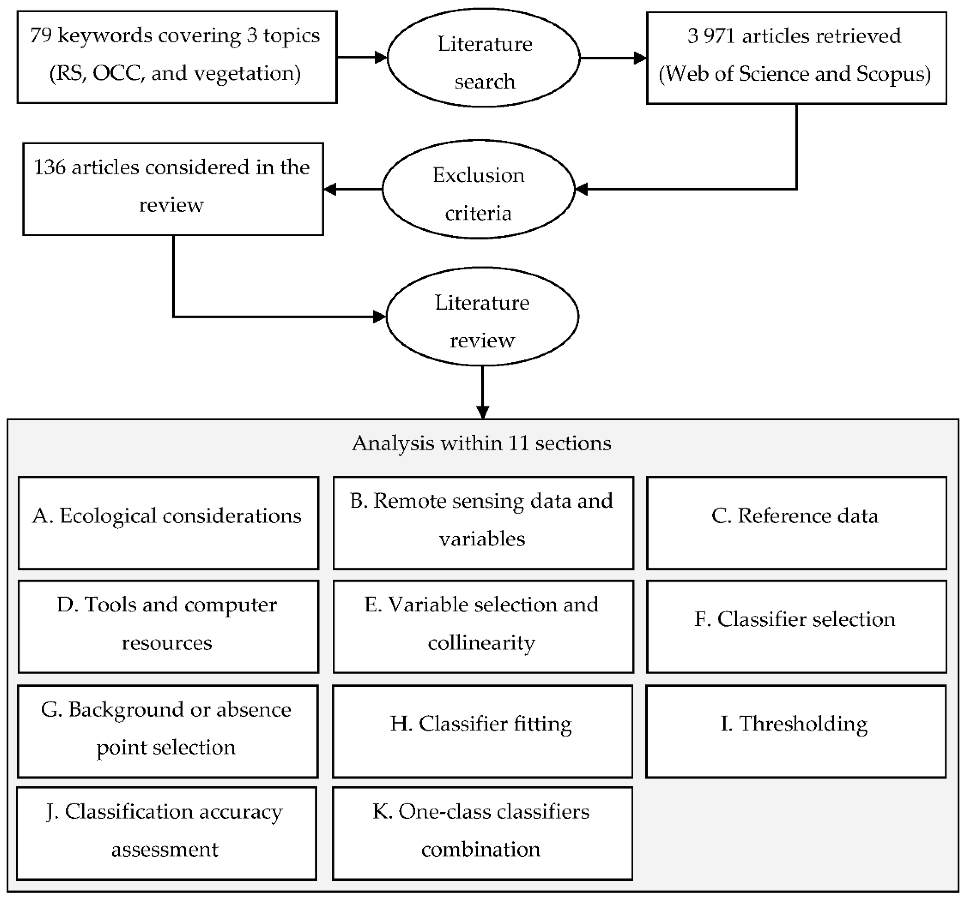
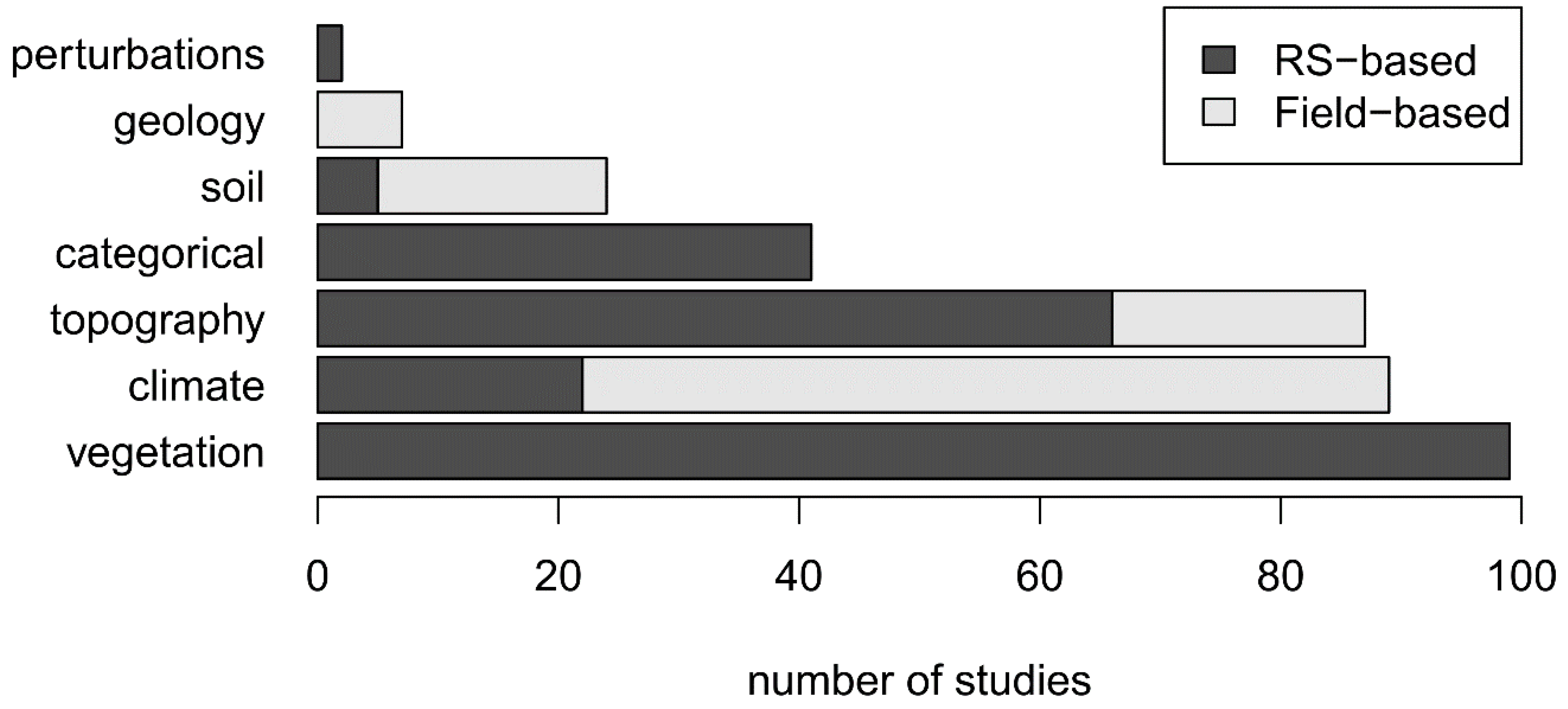
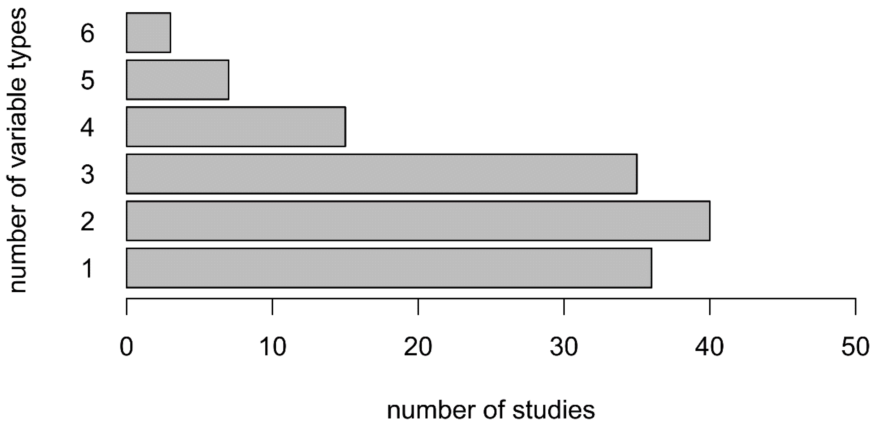
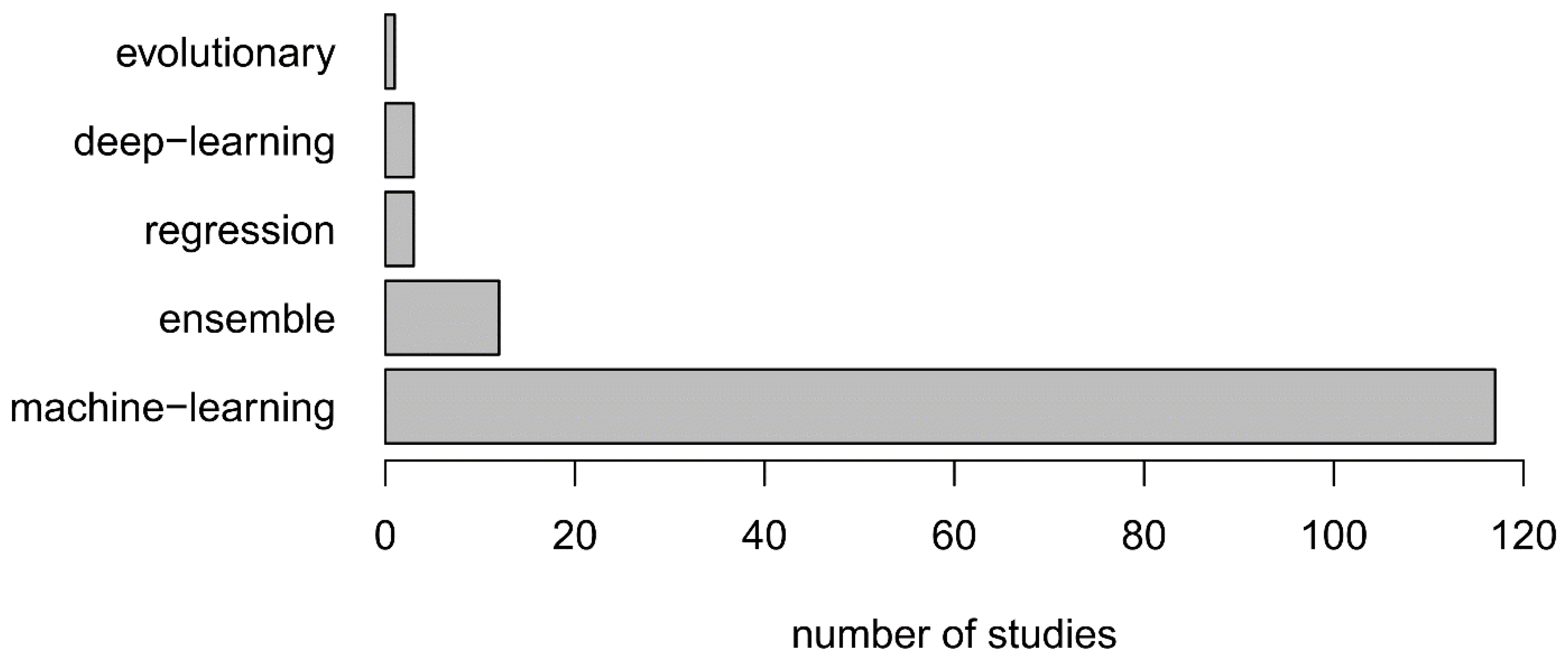
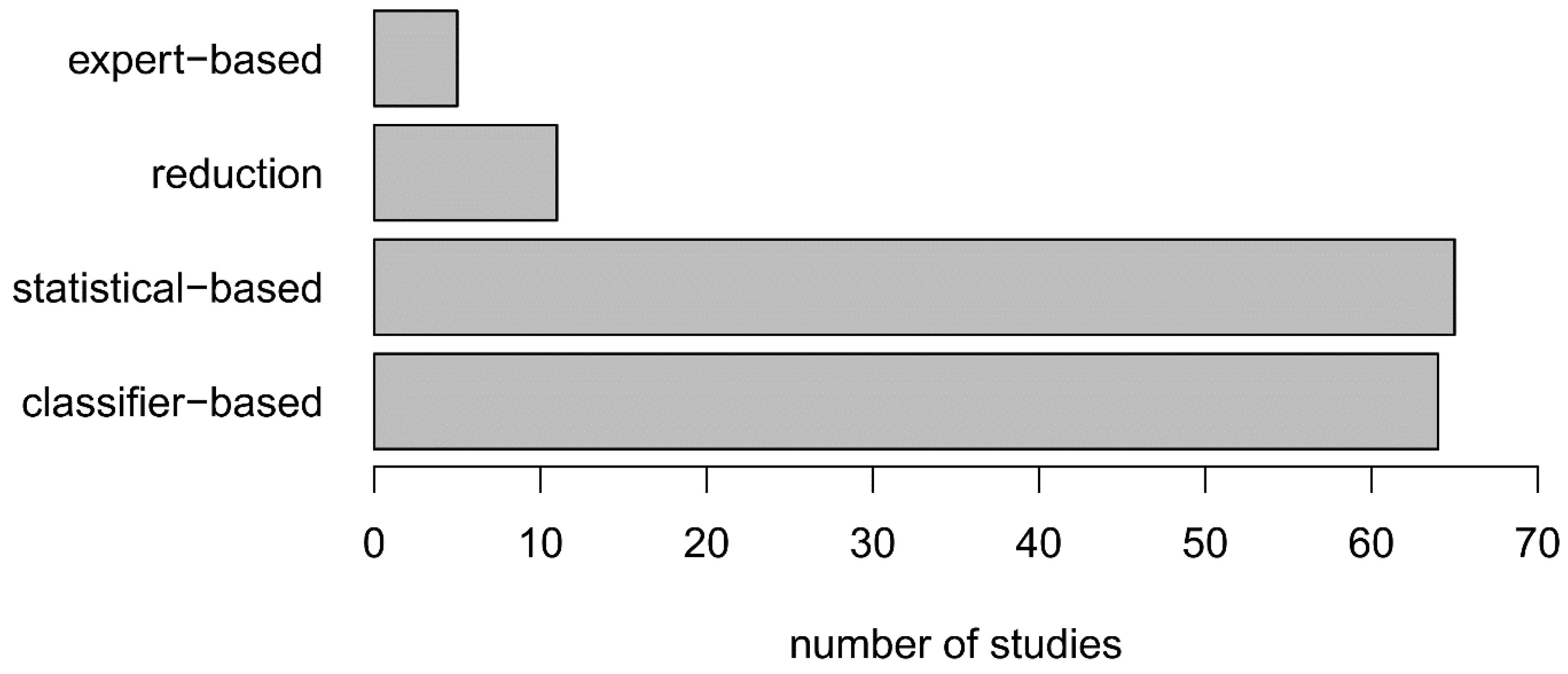
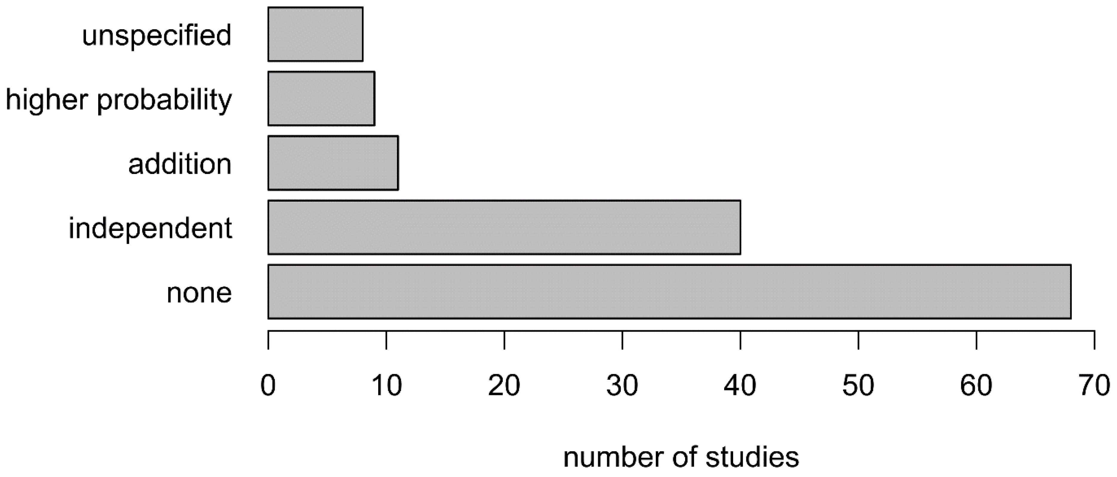
Table 1.
Keywords selected per topics for the literature searching. The asterisk (*) was used to retrieve variations of a term.
Table 1.
Keywords selected per topics for the literature searching. The asterisk (*) was used to retrieve variations of a term.
| Topics | |||
|---|---|---|---|
| Remote Sensing | One-Class Classifier | Natural Vegetations | |
| --------------------------------------- AND --------------------------------------------- | |||
 | remote * sens * | one-class classifier | plant * |
| remote-sens * | one class classifier | vegetation | |
| Earth observation | one-class model * | land cover | |
| satellite | one class model * | land-cover | |
| imagery | OCSVM | land-use | |
| orthophoto | OC-SVM | land use | |
| UAV | OCC | LULC | |
| drone | biased-SVM | landscape | |
| unmanned aerial | biased SVM | habitat | |
| aerial image * | GLM | alliance | |
| aircraft * | Generalized Linear Model | phytosociology | |
| airborne | AUC | ecosystems | |
| air-borne | TSS | Natura 2000 | |
| spaceborne | AIC | N2000 | |
| space-borne | SDM | EUNIS | |
| hyperspectral | S-SDM | functional traits | |
| hyper-spectral | Species distribution model * | dryland | |
| multispectral | Species classification | wetland | |
| multi-spectral | Maxent | peat * | |
| SAR | bog | ||
| radar | scrub * | ||
| LiDAR | shrub * | ||
| NDVI | heath * | ||
| MODIS | grass * | ||
| TRMM | meadow | ||
| Landsat * | tree * | ||
| Sentinel * | forest | ||
| Rapideye | wood * | ||
| ALOS * | phenology | ||
| RADARSAT * | biomass | ||
| SPOT * | biotope | ||
| SRTM | biome | ||
| Land Surface Temperature | conservation | ||
| ASTER | environment | ||
| Google Earth * | |||
| GEE | |||
| reflectance | |||
Table 2.
Topics, attributes, and categories used to analyze the articles selected (see Table S3 in Supplementary Materials for a complete description of categories).
Table 2.
Topics, attributes, and categories used to analyze the articles selected (see Table S3 in Supplementary Materials for a complete description of categories).
| Topic | Attribute | Categories |
|---|---|---|
| A. Ecological considerations | A1. Area of occupancy | Potential area; actual area |
| A2. Hierarchical level | Land cover; plant community; plant species | |
| A3. Number of classes | One class; multi-class | |
| A4. Site extent | Local (<1000 km2); regional (1000–100,000 km2); national; continental; global | |
| A5. Temporal monitoring | No; yes | |
| B. Remote sensing data and variables | B1. Sensor type | Multispectral; hyperspectral; SAR; LiDAR |
| B2. Platform type | Unmanned airborne; manned airborne; satellite | |
| B3. Spatial resolution | very high spatial resolution (<5 m); high spatial resolution (6–30 m); moderate spatial resolution (31–250 m); low spatial resolution (>251 m) | |
| B4. Acquisition frequency | Single; multi-temporal; annual time-series | |
| B5. Type of remote-sensing-based variable | Climate; soil; topography; vegetation; categorical; disturbance | |
| C. Reference data | C1. Reference type | Vegetation database; field collection; image collection |
| C2. Reference quantity | Very small (<10); small (10–50); moderate (50–100); large (100–1000); very large (>1000) | |
| D. Tools and computer Resources | D1. Software license | Open-source; commercial |
| D2. Computer location | Local computing; cloud computing | |
| E. Variable selection and collinearity | E1. Initial variable selection | Expert; literature; data mining |
| E2. Consideration of correlated variables | Classifier-based; expert-based; statistical-based; reduction | |
| F. Classifier selection | F1. Classifier type | Machine learning; ensemble classifier; deep learning; evolutionary algorithm |
| G. Background point selection | G1. Background point quantity | Small (<10,000); default (10,000); large (>10,000); unspecified; not applicable |
| G2. Consideration of spatial sampling | No; yes; not applicable | |
| G3. Area for background point selection | All landscapes; distribution area; natural areas; artificial areas; unspecified; not applicable | |
| G4. Consideration of area of occurrence | No; yes; not applicable | |
| H. Classifier fitting | H1. Type of classifier fitting | None; best performance; best transferability |
| H2. Type of absence data | Background; pseudo-absence; true absence; unspecified | |
| I. Thresholding | I1. Thresholding stage | Never; fitting/validation; categorical mapping |
| I2. Thresholding method | Default; statistical; expert-based; unspecified | |
| J. Classification accuracy assessment | J1. Consideration of spatial autocorrelation | No; yes |
| J2. Independent validation plots | No; yes | |
| J3. Accuracy assessment criterion | Best performance; spatial uncertainty; best transferability; expert-based | |
| K. One-class classifiers combination | K1. Classification combination method | Independent; higher probability; categorical map addition; unspecified |
Table 3.
Number of studies reviewed per type of occupancy area.
| Area of Occupancy | Number of Studies |
|---|---|
| Potential area | 65 |
| Actual area | 66 |
| Potential and actual areas | 5 |
Table 4.
Number of studies reviewed per hierarchical level of vegetation.
| Hierarchical Level | Number of Studies |
|---|---|
| Plant species | 102 |
| Plant community | 19 |
| Land cover | 15 |
Table 5.
Number of studies reviewed according to the acquisition frequency of remote sensing data used
Table 5.
Number of studies reviewed according to the acquisition frequency of remote sensing data used
| Acquisition Frequency | Number of Studies |
|---|---|
| Single | 67 |
| Multi-temporal | 34 |
| Annual time-series | 35 |
Table 6.
Percentages of studies reviewed that used given types of points for presence-only or presence/absence classifiers. Gray cells indicate correct types of points for each type of classifier.
Table 6.
Percentages of studies reviewed that used given types of points for presence-only or presence/absence classifiers. Gray cells indicate correct types of points for each type of classifier.
| Types of Points | ||||
|---|---|---|---|---|
| Type of Classifier | Background | Absence | Pseudo-Absence | Unspecified |
| Presence only | 44% | 15% | 28% | 13% |
| Presence/absence | 7% | 67% | 26% | 0% |
Table 7.
Number of studies reviewed using a classifier fitting to classify natural vegetation.
| Type of Classifier Fitting | Number of Studies |
|---|---|
| None | 89 |
| Best performance | 30 |
| Best transferability | 17 |
Table 8.
Number of studies reviewed using a thresholding stage during the classification process.
| Thresholding Stage | Number of Studies |
|---|---|
| None | 33 |
| Fitting/validation | 47 |
| Categorical mapping | 56 |
Table 9.
Number of studies reviewed that used spatially uncorrelated and independent validation plots during the classification accuracy assessment.
Table 9.
Number of studies reviewed that used spatially uncorrelated and independent validation plots during the classification accuracy assessment.
| Use of Spatially Uncorrelated Validation Plots | Use of Independent Validation Plots | |
|---|---|---|
| Yes | No | |
| Yes | 43 | 7 |
| No | 38 | 48 |
Publisher’s Note: MDPI stays neutral with regard to jurisdictional claims in published maps and institutional affiliations. |
© 2021 by the authors. Licensee MDPI, Basel, Switzerland. This article is an open access article distributed under the terms and conditions of the Creative Commons Attribution (CC BY) license (https://creativecommons.org/licenses/by/4.0/).
Share and Cite
MDPI and ACS Style
Rapinel, S.; Hubert-Moy, L. One-Class Classification of Natural Vegetation Using Remote Sensing: A Review. Remote Sens. 2021, 13, 1892. https://0-doi-org.brum.beds.ac.uk/10.3390/rs13101892
AMA Style
Rapinel S, Hubert-Moy L. One-Class Classification of Natural Vegetation Using Remote Sensing: A Review. Remote Sensing. 2021; 13(10):1892. https://0-doi-org.brum.beds.ac.uk/10.3390/rs13101892
Chicago/Turabian StyleRapinel, Sébastien, and Laurence Hubert-Moy. 2021. "One-Class Classification of Natural Vegetation Using Remote Sensing: A Review" Remote Sensing 13, no. 10: 1892. https://0-doi-org.brum.beds.ac.uk/10.3390/rs13101892
Note that from the first issue of 2016, this journal uses article numbers instead of page numbers. See further details here.