Article

Use of GNSS Tropospheric Delay Measurements for the Parameterization and Validation of WRF High-Resolution Re-Analysis over the Western Gulf of Corinth, Greece: The PaTrop Experiment

by
Nikolaos Roukounakis
1,2,3,*,
Dimitris Katsanos
1,
Pierre Briole
2,
Panagiotis Elias
4,
Ioannis Kioutsioukis
3,
Athanassios A. Argiriou
3 and
Adrianos Retalis
1
1
Institute for Environmental Research and Sustainable Development, National Observatory of Athens, 15236 Athens, Greece
2
Laboratoire de Geologie, UMR CNRS ENS PSL 8538, 24 rue Lhomond, CEDEX 05, 75231 Paris, France
3
Laboratory of Atmospheric Physics, Department of Physics, University of Patras, 26500 Patras, Greece
4
Institute for Astronomy, Astrophysics, Space Applications and Remote Sensing, National Observatory of Athens, 15236 Athens, Greece
*
Author to whom correspondence should be addressed.
Remote Sens. 2021, 13(10), 1898; https://0-doi-org.brum.beds.ac.uk/10.3390/rs13101898
Submission received: 17 March 2021 / Revised: 1 May 2021 / Accepted: 7 May 2021 / Published: 13 May 2021
(This article belongs to the Special Issue Satellite Observation for Atmospheric Modeling)

Abstract

:
In the last thirty years, Synthetic Aperture Radar interferometry (InSAR) and the Global Navigation Satellite System (GNSS) have become fundamental space geodetic techniques for mapping surface deformations due to tectonic movements. One major limiting factor to those techniques is the effect of the troposphere, as surface velocities are of the order of a few mm yr−1, and high accuracy (to mm level) is required. The troposphere introduces a path delay in the microwave signal, which, in the case of GNSS Precise Point Positioning (PPP), can nowadays be partly removed with the use of specialized mapping functions. Moreover, tropospheric stratification and short wavelength spatial turbulences produce an additive noise to the low amplitude ground deformations calculated by the (multitemporal) InSAR methodology. InSAR atmospheric phase delay corrections are much more challenging, as opposed to GNSS PPP, due to the single pass geometry and the gridded nature of the acquired data. Thus, the precise knowledge of the tropospheric parameters along the propagation medium is extremely useful for the estimation and correction of the atmospheric phase delay. In this context, the PaTrop experiment aims to maximize the potential of using a high-resolution Limited-Area Model for the calculation and removal of the tropospheric noise from InSAR data, by following a synergistic approach and integrating all the latest advances in the fields of remote sensing meteorology (GNSS and InSAR) and Numerical Weather Forecasting (WRF). In the first phase of the experiment, presented in the current paper, we investigate the extent to which a high-resolution 1 km WRF weather re-analysis can produce detailed tropospheric delay maps of the required accuracy, by coupling its output (in terms of Zenith Total Delay or ZTD) with the vertical delay component in GNSS measurements. The model is initially operated with varying parameterization, with GNSS measurements providing a benchmark of real atmospheric conditions. Subsequently, the final WRF daily re-analysis run covers an extended period of one year, based on the optimum model parameterization scheme demonstrated by the parametric analysis. The two datasets (predicted and observed) are compared and statistically evaluated, in order to investigate the extent to which meteorological parameters that affect ZTD can be simulated accurately by the model under different weather conditions. Results demonstrate a strong correlation between predicted and observed ZTDs at the 19 GNSS stations throughout the year (R ranges from 0.91 to 0.93), with an average mean bias (MB) of –19.2 mm, indicating that the model tends to slightly underestimate the tropospheric ZTD as compared to the GNSS derived values. With respect to the seasonal component, model performance is better during the autumn period (October–December), followed by spring (April–June). Setting the acceptable bias range at ±23 mm (equal to the amplitude of one Sentinel-1 C-band phase cycle when projected to the zenithal distance), it is demonstrated that the model produces satisfactory results, with a percentage of ZTD values within the bias margin ranging from 57% in summer to 63% in autumn.

1. Introduction

In recent years, and with the advent of high-performance computer systems (HPCs), high-resolution Limited-Area Model (LAM) applications are being increasingly utilized, both in operational weather forecasting and in atmospheric research as weather re-analysis tools. Atmospheric studies involving dynamical downscaling with high-resolution LAMs focus either on the estimation of local meteorological parameters and climatic patterns (detailed wind fields, precipitation characteristics, local humidity etc.) or on the actual validation of the model used, depending on its parameterization and comparison with observational data. Common LAMs which have been employed for research and climate re-analysis include MM5, RAMS and WRF. In recent years, WRF [1] has become the most widely used model, due to its versatility as an open-source package supported by a large user community and the fact that it can be operated efficiently on parallel computing platforms, making it suitable for use in a wide range of applications at high horizontal resolutions (down to 1 km or less).
The use of high-resolution regional weather models (LAMs) nested within coarser, global, weather models is currently gaining ground in the domain of satellite imagery, as the precise knowledge of meteorological parameters along the lower atmosphere is extremely useful for the correction of remote sensing data, and in particular Synthetic Aperture Radar (SAR) interferograms [2,3,4,5,6,7,8]. Tropospheric stratification and short wavelength spatial turbulences produce a phase delay, and consequently an additive noise to the low amplitude ground deformations calculated by the multitemporal InSAR methodology. The removal of the atmospheric phase screen (APS) is a challenging task (as opposed to GNSS, for example, which uses signals in the same microwave bandwidth), due to several reasons, including the small number of satellites, the single pass geometry and the gridded nature of the acquired data. Several methods have so far been pursued to mitigate the tropospheric delay in InSAR data, including local atmospheric data collection [9], GNSS zenithal delay estimations [10,11,12], satellite multispectral imagery analysis [13,14,15], empirical phase/topography estimations [8,16,17,18], and zenithal delay estimations from Global Atmospheric Models (GAMs) [19,20,21]. These methods have their limitations, as they rely either on local data assimilation, which is rarely available at the desired spatial resolution, or on empirical estimations which are difficult in situations where deformation and topography are correlated.
The advantage of using LAMs over other techniques is the ability to produce detailed delay maps at high spatial resolution (down to 1 km), by estimating atmospheric parameters, such as water vapour and temperature, in the entire vertical column which cannot be easily estimated otherwise. Foster et al. [2,3], employed the MM5 regional model at high horizontal resolution (3 km) to obtain tropospheric delay fields over the Island of Hawaii and Mount St. Helens in the U.S. with mixed success, as the model configuration failed to accurately predict tropospheric delays at shorter wavelengths (under 8 km) in most cases. Wadge et al. [5], performed tropospheric delay corrections, using the Unified Regional Mesoscale Model at high-resolution over Mount Etna in Sicily. The study concluded that LAMs show a promising potential in calculating the path delay due to tropospheric water vapor in regions of high relief and high water vapour variance such as Mount Etna, and that the model was able, under certain conditions, to simulate local modifications of water vapour content by mechanisms such as land–sea breezes. More recently, Bekaert et al. [8] produced tropospheric delay fields with the WRF regional model over three test-regions with complex topography. The model is nested at 7 km horizontal resolution and is initiated with data from the Global Forecast System (GFS). Results are compared with tropospheric delays obtained with other state-of-the-art methods, including MERIS and MODIS spectroscopy, ERA-Interim, and both the conventional linear and power-law empirical methods. The statistical analysis demonstrated that spectrometers provided the largest RMSE reduction, but only under daylight and cloud-free conditions. Phase-based methods (linear and power-law) outperformed the weather models in regions where tropospheric delays were correlated with topography, but in regions where this was less apparent, due to atmospheric turbulence and dynamic local weather, weather models offered better performance. On the whole, recent studies which employ LAMs for the removal of tropospheric artifacts from InSAR data demonstrate the ability of weather models to calculate detailed tropospheric delay fields under any atmospheric conditions and at the exact times of SAR acquisitions, thus offering a reliable tool for tropospheric corrections. Indeed, it is evident that in cases of atmospheric turbulence and dynamic local weather, weather models can offer better performance [8,22]. However, the generic configuration and parameterization of the LAMs used in these studies have prohibited, so far, the full exploitation of the method.
Our work aims to maximise the potential of using LAMs for the calculation and removal of the tropospheric component from SAR interferograms by evaluating a novel methodology which integrates the latest advances in the fields of remote sensing meteorology (GNSS and InSAR) and high-resolution Numerical Weather Forecasting (WRF). Our research focuses on the interaction of the three aforementioned techniques in the area of the western Gulf of Corinth in Greece and aims to optimise their synergic output by identifying strengths, weaknesses and uncertainties with respect to the measurement of zenithal tropospheric delays. We investigate the extent to which a high-resolution WRF 1 km re-analysis can produce detailed tropospheric delay maps of the required accuracy, by coupling its output, in terms of Zenith Total Delay (ZTD), with the vertical delay component in GNSS measurements. One of the main limitations in the estimation of precise ZTD fields is the presence of highly variable water vapour signals, both in space and in time, which are exhibited in the differential atmosphere as densely distributed short-wavelength phase gradients. It is expected that the high horizontal resolution and dense vertical layering of the model will be capable of capturing near-surface atmospheric processes such as sea breezes, orographic flows, turbulent boundary layer interactions, etc., which influence the distribution of water vapour in settings of complex topography, thus overcoming this important limitation.
The model is initially operated with varying parameterization in order to demonstrate the best possible configuration, with GNSS measurements providing a benchmark of real atmospheric conditions. The two datasets (predicted and observed) are compared and statistically evaluated for a period of one year, in order to investigate the extent to which meteorological parameters that affect ZTD, can be simulated accurately by the model under different weather conditions. In the next phase, we compare twenty Sentinel-1A interferograms with differential delay maps at the LOS produced by WRF re-analysis. Results of the second phase of the experiment are presented in a separate paper.

2. Materials and Methods

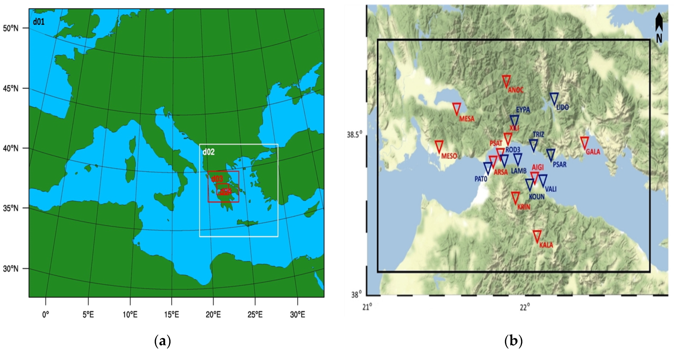
2.1. Description of the Study Area and Experimental Setup

The experiment, with the code name PaTrop (Patras–Troposphere), was implemented for providing the data needed for this study. The PaTrop test site covers an area of approximately 150 × 90 km in the region of the Western Gulf of Corinth (GoC). It is identified as a site of intense geophysical activity and forms one of the most active intra-continental rifts in the world. Geodetic studies conducted over the past 20 years based on GNSS and InSAR observations have revealed North-South extension rates up to 1.5 cm yr−1 [23,24], one of the highest worldwide. In this context, the existing network of permanent GNSS stations used by the Corinth Rift Laboratory (CRL) to continuously monitor surface displacements in the area could be exploited for the needs of our study. A network of nineteen permanent Topcon GB1000 and Topcon Net G3A GNSS receivers fitted with Topcon PG-A1 antennas provided the GNSS data and the subsequent in-situ zenithal tropospheric delay measurements, as shown in Figure 1b. Ten of those receivers were installed during the PaTrop campaign in order to expand the existing CRL network. The stations’ locations were selected to cover the whole geographic extent of the study area, while capturing a variety of different topographical and meteorological conditions (i.e., coastal, inland, or mountainous terrain), at elevations between 0 and 1020 m above sea level (ASL). This was deemed necessary, in order to account mainly for water vapour variations resulting from orographic, coastal, and frontal gradients that could be present.
Concurrently with the field campaign, the modelling setup and configuration was also implemented. The primary objective of PaTrop is to couple the zenithal tropospheric delay (ZTD) derived from GNSS data with the ZTDs derived from the output of a high-resolution meteorological model (WRF), in order to investigate the model’s capability to reproduce the tropospheric conditions that contribute to the noise signal (in particular the highly variable water vapour distribution), and provide a benchmark of real observational data for validating the model output. The Weather Research and Forecasting (WRF) model [1] is a widely used open-source weather forecasting and re-analysis model that can be configured by the user according to the specific needs of each study. WRF has a proven record of producing high-resolution meteorological simulations down to a scale of hundreds of meters. It can be installed and operated in parallel mode using multi-processor computing resources, and therefore computational time can be greatly reduced for high-resolution simulations covering large geographical areas, such as PaTrop. Keeping the spatial resolution of the inner domain at 1 km, a series of re-analysis runs were produced to demonstrate the best possible configuration for our study, which is an approach supported theoretically and practically to tackle uncertainties in high-resolution modelling [25,26]. The parametric analysis was performed for a two-week period (17–29 June 2016), during which the output of five different model configurations was tested against GNSS tropospheric measurements from the network of permanent stations in the study area. The optimum model configuration which resulted from the analysis was subsequently employed to provide the data for the main part of the PaTrop experiment. In order to establish the correlation between the observed and predicted time series, the following metrics are used, which give us a quantitative indication of the prediction skill of different model schemes with respect to the GNSS network dataset:
Mean   Bias   ( MB ) :   σ ¯ = f i o i N
Mean   Absolute   Bias   ( MAB ) :   σ ¯ = f i o i N
Root   Mean   Square   Error   ( RMSE ) :     R M S E = f i o i 2 N
Pearson   Correlation   Coefficient   ( R ) :     r = 1 N i f i f ¯ o i o ¯ σ f σ o
where fi denotes the model value, oi the observational value, N is the number of pairs in the examined time series, σf is the standard deviation of the model values and σo the standard deviation of the observations.

2.2. Data Processing

Processing of the GNSS data started after the end of the experimental campaign and included calculations of zenith tropospheric delays (ZTDs) every 30 min using the JPL NASA Precise Point Positioning (PPP) GIPSY-OASIS 6.4 software. High-precision International GNSS Service (IGS) final orbit data were used, while the quality of the sites ensured that multipath effects would not bias the estimated ZTDs. Static tropospheric processing with no mapping function was used, and a priori ZHD was estimated from an elevation-dependent function. It was intended to use a simple set of parameters in order to compare the WRF model output with a geometrical GNSS calculation which does not assimilate data from external sources (i.e., weather models). The exact settings of the processing protocol used are listed in Table 1.
With regards to the processing of WRF tropospheric data, values of surface pressure (Ps), as well as air temperature and water vapour pressure (T, pv) in the vertical column (for each of the 45 vertical pressure levels) were derived every 30 min, at hh:00 and hh:30 h, at the nearest 1 km grid point from each GNSS station, to coincide with the observational time series. An automatic routine calculates the “dry” and “wet” delay terms separately, from the three parameters (Ps, T, pv), together with the point elevation and layer heights, finally adding up the two to calculate the ZTD value [27,28,29]:
ZTD (mm) = ZHD + ZWD
With:
ZHD = 2.2779 ± 0.0024   P s   / f λ ,   H
where   P s   is the total pressure (mbar) at the Earth’s surface, and:
f   λ ,   H = 1     0.00266   c o s 2 λ     0.00028 H    
accounts for the variation in gravitational acceleration with latitude λ and the height H of the surface above the ellipsoid (in km).
And:
ZWD = 0.382 ± 0.004 K 2 m b a r 1 p v T 2 d z
where   p v   is the water vapour pressure (mbar), and T the air temperature (K), integrated along the zenith path z.
WRF derived ZTDs were calculated at the exact elevation of the GNSS receiver, by vertically interpolating these parameters, thus minimising errors due to vertical height differences between the two datasets. Figure 2 illustrates graphically the GNSS-WRF geometry used in the calculation of the respective ZTD values.

2.3. Model Configuration and Parameterization of Physical Components

For the high-resolution dynamical downscaling simulation performed with WRF v 3.7.1 over the PaTrop area of the western Gulf of Corinth, four nested domains were used (d01–d04), with a horizontal resolution of 27, 9, 3 and 1 km, respectively, as shown in Figure 1a; two-way nested, i.e., feedback from nest to its parent domain. The vertical layer distribution consists of 45 sigma levels up to a height of about 20 km (0.1 hPa), with bottom layers being more densely populated. Boundary conditions for the model initialization were taken from the ERA-Interim global climate re-analysis database, with a 75 km horizontal resolution, 35 vertical layers and 6 h temporal resolution. The model was initiated every day from the ERA-Interim input data at 18:00 local time, producing 30 h simulations with the first 6 h being spin-up time. Model output was recorded every 30 min, from which Zenith Hydrostatic Delays (ZHD) and Zenith Wet Delays (ZWD) were calculated as previously described. Land-use categories were taken from USGS 24-category data, which are available for different horizontal resolutions (10′, 5′, 2′, 30″). The initial land topography dataset used was the Global 30 Arc-Second Elevation Model (GTOPO30) provided by United States Geological Survey (USGS), with a 30″ resolution for the smaller domain (d04), and coarser resolutions (10′, 5′, 2′) for domains d01–d03, respectively. However, in order to test the impact of a more detailed topography on the re-analysis output, a high-resolution terrestrial dataset of d04 was later introduced (ASTER 1″ global GDEM v2), with a horizontal grid of 30 m.
For the model physical and dynamical parameterization, five different schemes were tested, in order to evaluate each scheme for its forecasting skill. There have been numerous studies validating the output of different model configurations with observations under specific conditions [25,30,31,32], showing that globally there is no optimal scheme, but rather different schemes produce better results with respect to application, domain, season, variable, etc. Therefore, a model parameterization test was performed for a two-week period (17–29 June 2016), during which the output of the five different model configurations was tested against GNSS tropospheric measurements from 16 permanent stations in the study area (d04).
The schemes were selected based on existing studies where similar high-resolution WRF simulations were used. All five schemes use the same parameterization for radiation physics (shortwave and longwave) and cumulus convection. In the first three schemes (MOD1, MOD2 and MOD3), cumulus convection is modelled in the 27 km domain according to the Kain–Fritsch scheme [33,34]. The cumulus scheme is not activated for the 9, 3 and 1 km domains, because at higher resolution the model can theoretically resolve convection explicitly [34]. In schemes MOD4 and MOD5, cumulus convection was turned on for d02 (9 km) in order to test the effect of cumulus parameterization in a smaller domain. Convection plays an important role for cloud formation and is controlled by micro-scale processes such as mixtures of updrafts and downdrafts. These simulated convective features are less distinguishable as model resolution becomes coarser; therefore, parameterization becomes necessary, although computationally demanding. Furthermore, in locations such as the Gulf of Corinth, where cloud formation is strongly influenced by the intense topography (land-sea contrasts and mountainous features), it is expected that cumulus parameterization in the 9 km domain will better represent the effects of sub-grid scale processes on the grid variables, particularly in the case of squall line formation, thunderstorms and other strong convection events [35].
Longwave radiation was simulated by the RRTM scheme [36] with the default diffusion scheme selected. The shortwave radiation was simulated by the Dudhia scheme [37]. Both are typical schemes for high-resolution WRF simulations. With respect to microphysics, land surface and planetary boundary layer options, the model was originally configured with the basic options for a less computationally demanding ERA-Interim dynamical downscaling at 1 km horizontal resolution. In the second scheme (MOD2), the microphysics scheme was changed to Morrison double-moment [38], in order to investigate the effect of a more complex model which uses double-moment ice, snow, rain and graupel for cloud-resolving simulations [25,39]. In the third scheme (MOD3), the same configuration as MOD2 was used, with a change in land surface parameters, in which the Pleim–Xiu land surface model and Pleim–Xiu surface layer physics was used [40,41]. In the fourth scheme (MOD4), the same configuration as MOD3 was used, this time with the cumulus scheme activated in the second domain (9 km), as explained above. Finally, the fifth scheme (MOD5) used the parameterization of Zhang et al. [42], as it refers to a study with similar dynamical downscaling characteristics (input dataset and horizontal resolution), performed over a complex terrain with land-sea contrasts (Hong Kong island). The parameters changed compared with the previous schemes were microphysics (SBU-YLin model was used, a sophisticated scheme that has ice, snow and graupel processes, suitable for real-data high-resolution simulations) [43], PBL scheme (YSU used in conjunction with SBU-YLin), and surface layer scheme (MM5 similarity). The NOAH model was used for land surface. Again, cumulus convection is activated in the second domain (9 km). Table 2 lists the parameterization used in each scheme.

3. Results

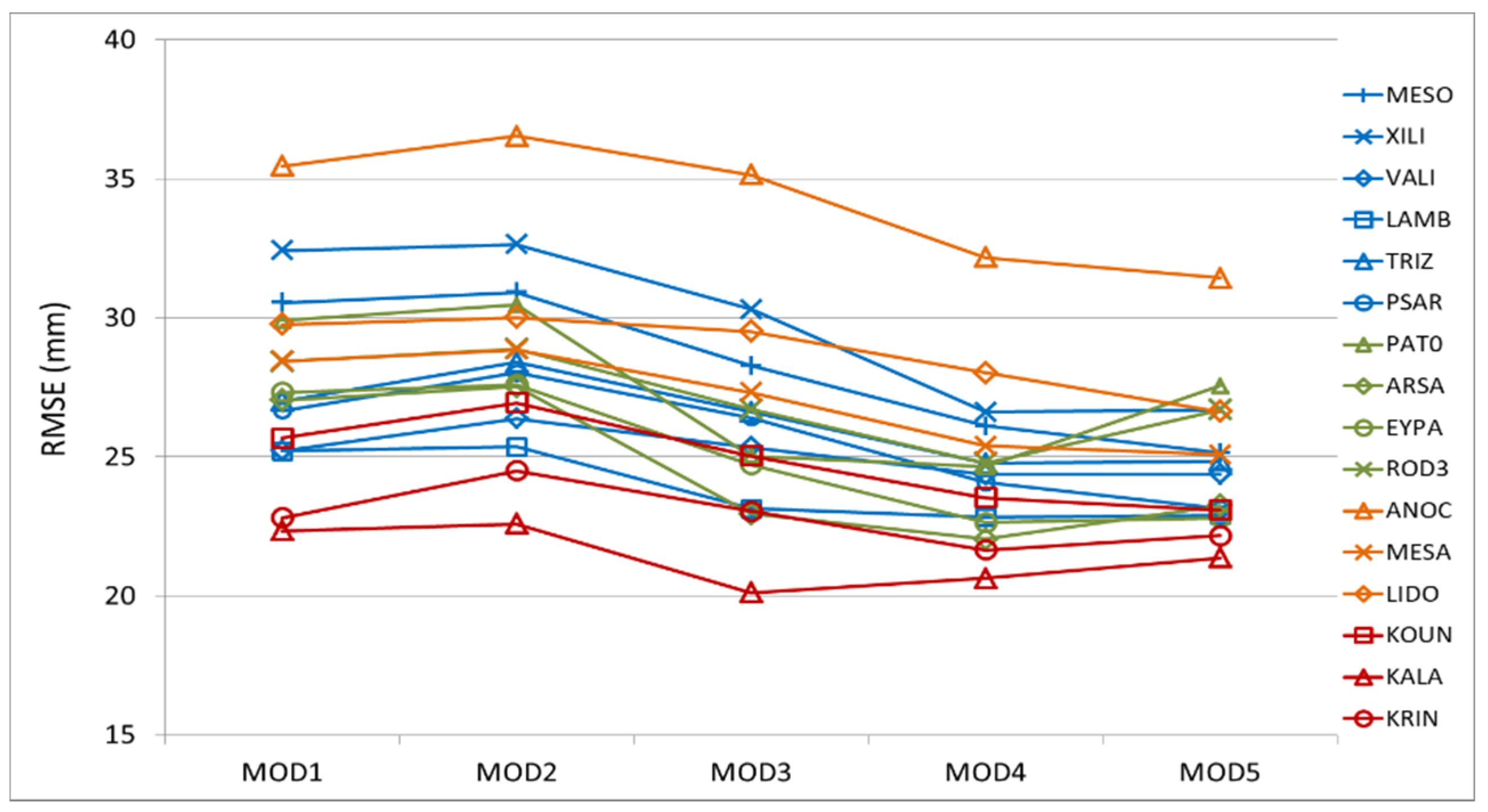
3.1. Parametric Analysis and Evaluation of WRF Schemes with GNSS Data

The parametric analysis was performed for a two-week period (17–29 June 2016), with the aim to test the forecasting skill of different WRF parameterization schemes. Tropospheric data (i.e., ZTD values) from the CRL GNSS network provided the benchmark for the analysis, for comparison with ZTDs derived from WRF at the nearest grid point. The selection of the test period for the parametric analysis was based on weather conditions (i.e., high temperatures and the occurrence of a convective storm event during the last days of June), which theoretically would produce a high degree of ZTD variability. Out of the 19 GNSS stations of the PaTrop network, 16 were fully operational during this period, while three (GALA, PSAT and AIGI) were not included in the analysis. Time series of WRF MOD1-MOD5 vs. GNSS ZTDs at 4 PaTrop stations (KALA, MESA, EYPA, PSAR) for the test period (17–29 June 2016) are presented in Figure 3, and corresponding bias plots of predicted (WRF MOD5) minus observed (GNSS) ZTDs are shown in Figure 4. Temporal resolution is 30 min and all times are in UTC.
Results at most stations exhibit a strong correlation between WRF derived ZTDs and GNSS values, with the exception of the last two days of the experiment (28–29/6) where the model shows significant deviation from the observed data. All schemes seem to follow the overall trend (including the storm event of 25–26 June). The Correlation Coefficient R at the 16 locations, for the test period, ranges from 0.57 at LIDO to 0.85 at PAT0, both with the MOD5 scheme (Table 3). Overall, MOD3, MOD4 and MOD5 exhibit the strongest correlation, with MOD5 having the highest average R score (0.74).
The model in general seems to slightly underestimate the observed data, especially for high ZTD values. Mean bias (MB) values indicate that, on average, this offset ranges from −14.9 mm (MOD1) to −11.6 mm (MOD5). Mean absolute bias (MAB) is a measure of the average absolute error between the two time series. Mean absolute bias values at the 16 locations range from about 15 mm at KALA to 26 mm at ANOC. Schemes with more sophisticated physical parameterization, better suited for high-resolution re-analysis (MOD4 and MOD5) exhibit the lowest overall MAB values (19.5 mm). Similarly, root mean square error (RMSE) values range from 21 mm at KALA to 31 mm at ANOC. Figure 5 illustrates the RMSE spread between the 16 points, for each model configuration. It is shown that schemes with a more complex physical parameterization (MOD4 and MOD5) exhibit lower RMSE values, as well as narrower spread than initial WRF configurations. Results also indicate that the RMSE distribution is more homogeneous among coastal and inland stations (blue and green colours), than stations in mountainous locations (orange and red). This finding could be related to the specific meteorological conditions which characterize regions with intense topography, as well as the fact that input data (e.g., measurements from surface stations) injected into the model as initial conditions, may be sparse in certain remote locations, leading to a poorer model prediction skill in these areas.
A graphical summary of validation metrics for MOD5 is found in Figure 6. We observe that although R is decreasing with increasing station elevation (as previously discussed), MAB and RMSE are not significantly increasing, which is a result of lower absolute ZTD values at higher altitudes where the tropospheric layer is thinner.
Under turbulent and humid atmospheric conditions (e.g., afternoon of 25 June), different schemes behave in different manners. Two separate groups can be distinguished (MOD1, MOD2 and MOD3 vs. MOD4 and MOD5), with the second group exhibiting a better prediction skill, possibly as a result of the Kain–Fritsch cumulus convection scheme being turned on at the 9 km domain. A significant deviation event can also be distinguished during the second half of 28 June, where the model produces a sudden “drop” in all stations (of the order of 60–120 mm) in relation to the observed ZTDs.

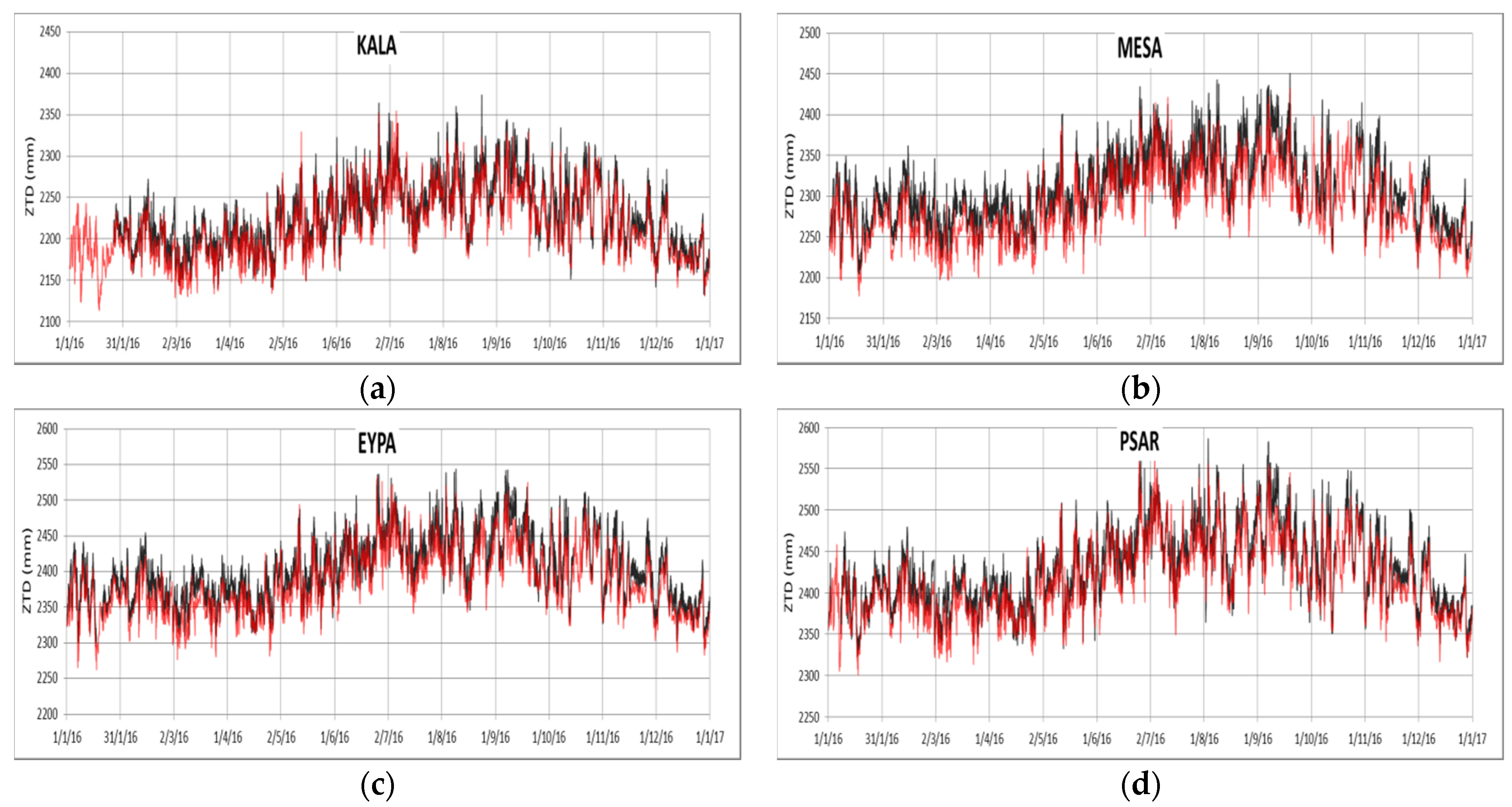
3.2. Validation of WRF Derived Tropospheric Delay Maps with GNSS ZTD Measurements for the PaTrop Period (January–December 2016)

Following the initial configuration of the WRF model and parameterization based on the short-scale analysis, as described in the previous section, the main part of the PaTrop experiment extends into a whole year of validation of model re-analysis output with the use of observational tropospheric data from the CRL GNSS network in the Western Gulf of Corinth. The WRF scheme which provided the best simulation results based on the parametric test was selected (MOD5), having a more complex physical parameterization, and hence being better suited for high-resolution re-analysis simulations. This includes: the SBU-YLin microphysics model, with a more sophisticated scheme for ice, snow, rain and graupel processes in the lower troposphere; the NOAH land surface model; the MM5 similarity scheme for surface layer physics; and the YSU planetary boundary layer model. In addition, MOD5 uses a cumulus convection scheme in both the 27 km and 9 km domains, thus simulating processes such as convective fluxes and the associated evaporation or condensation of water more coherently over a complex terrain with land-sea contrasts. The MOD5 output, represented as Zenith Total Delay (ZTD) values calculated from specific atmospheric parameters (surface pressure, air temperature and water vapour profiles) over the entire 1 × 1 km grid is validated against a dataset of GNSS derived ZTD values, providing point measurements at the 19 points where the stations are located.
Macroscopically, the two ZTD datasets are closely correlated in all 19 locations (Figure 7), with values peaking during the warm months (July–September) and subduing during the cold period (December–March), as expected (ZTD is proportional to surface pressure and air temperature which both increase during summer). It is also visible from the oscillating pattern of the time series that in absolute terms the tropospheric delay signal shows a higher degree of variability during the second half of the year than during the first half, as a result of a combination of more intense temperature and water vapour fluctuations. Bias plots of predicted (WRF) minus observed (GNSS) ZTDs (Figure 8) indicate a slightly stronger bias during the warm period. For a more detailed analysis of the correlation between the two datasets, the same statistical indices are used as in the physical parameterization study (R, MB, MAB, RMSE), which give us a quantitative indication of the accuracy and variability of the model prediction with respect to the dataset of the GNSS monitoring network. A summary of the regression statistics for the whole period of study is presented in Table 4.
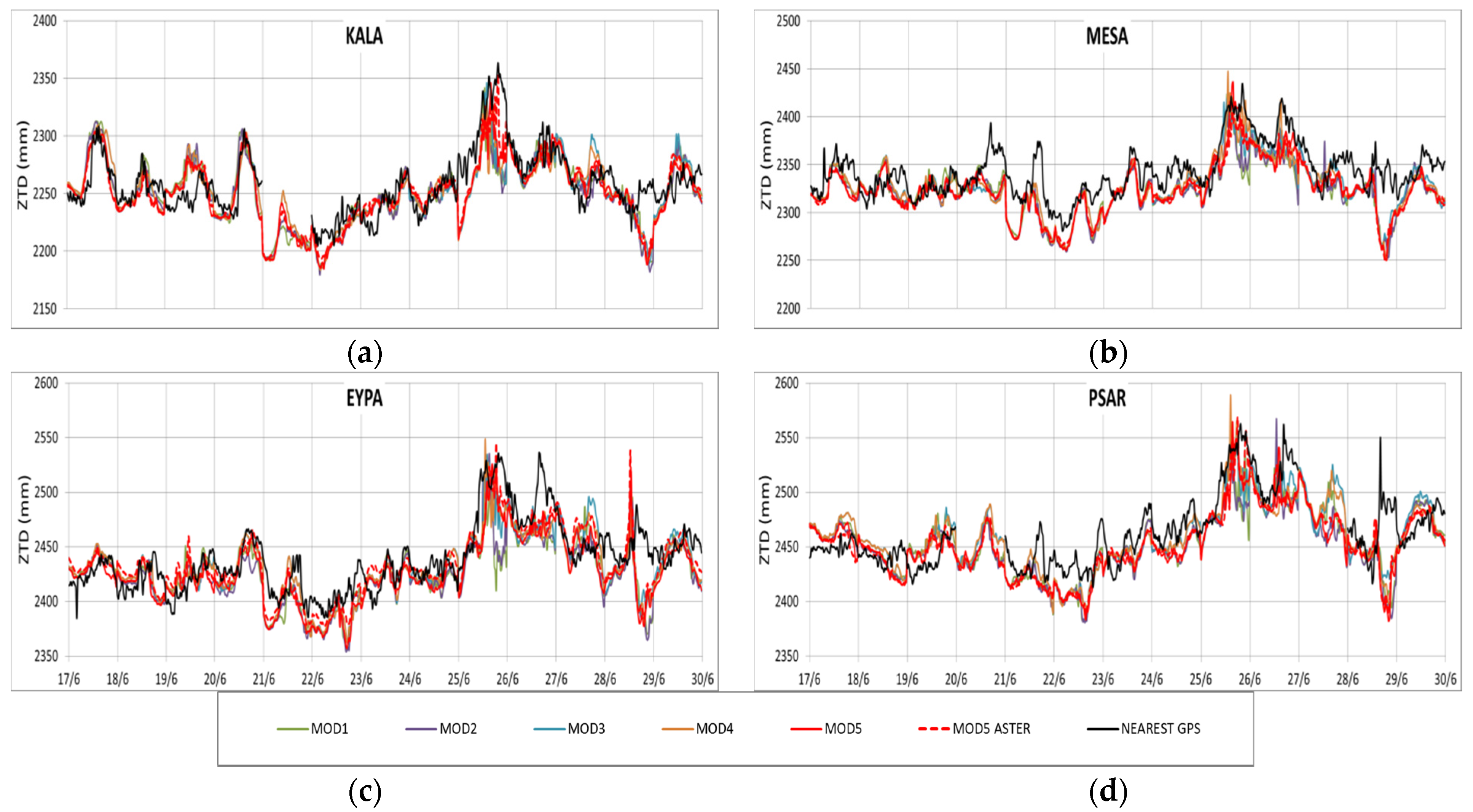
  • The Pearson correlation co-efficient R measures the extent to which two variables are linearly related. An R value of 1 means that the two variables are perfectly positively linearly related and that the points in the scatter plot lie exactly on a straight line (y = x). The R at the 19 locations, for the entire annual time series, ranges from 0.91 to 0.93, i.e., it is fairly uniform, indicating that the model’s variability matches the variability of the observed tropospheric delay about 90% of the time.
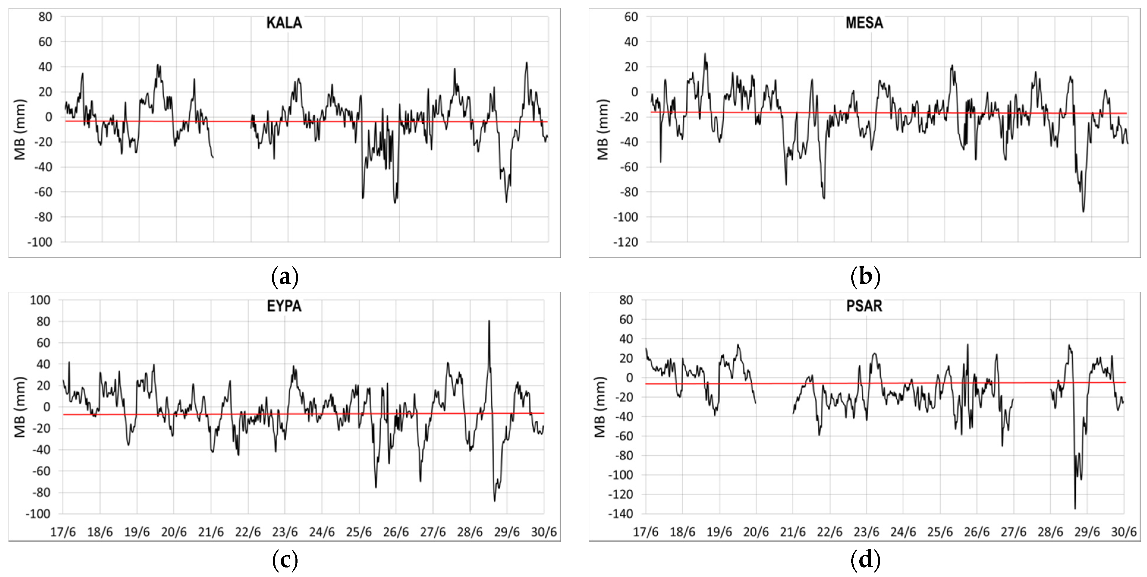
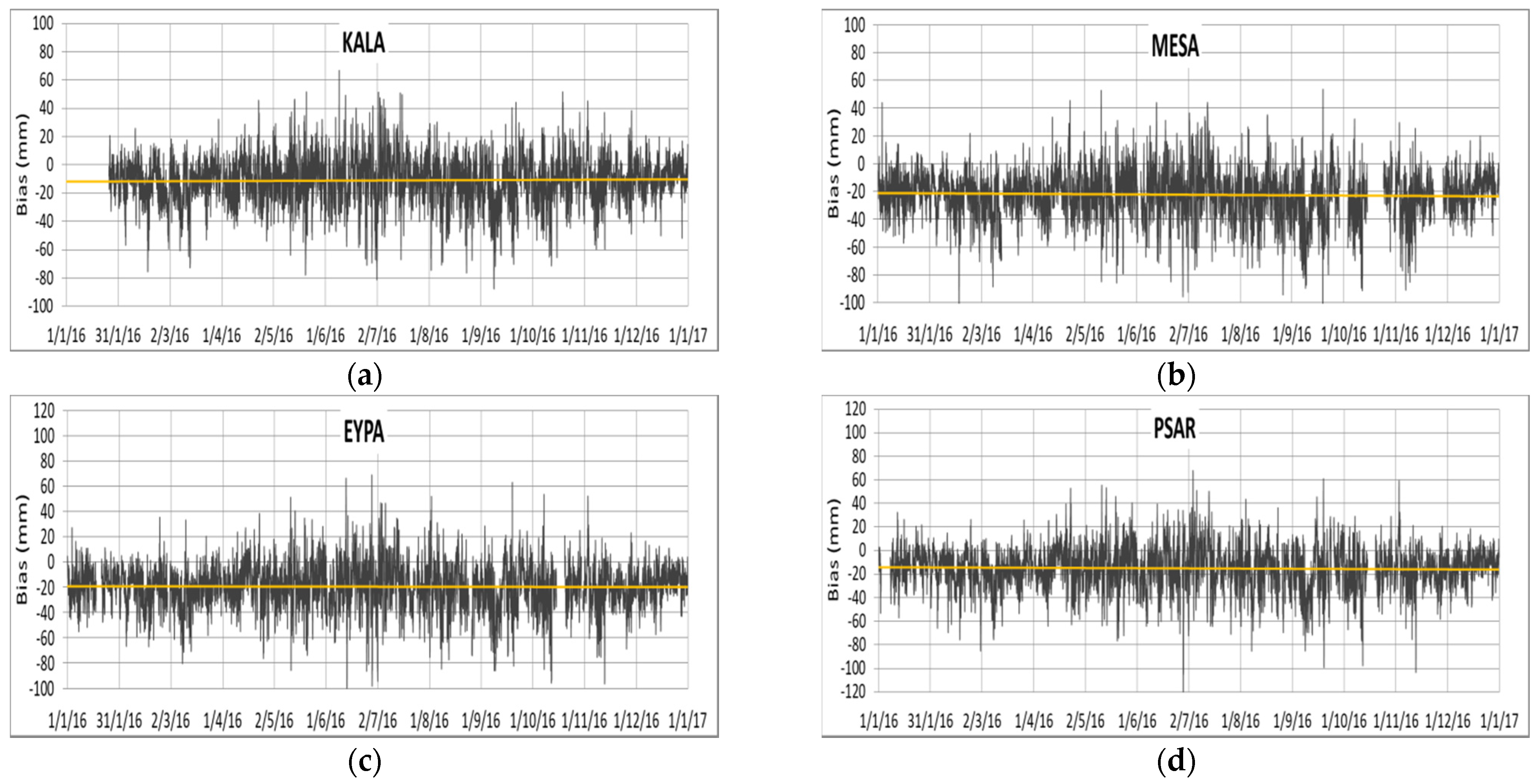
  • Mean bias (MB) is a measure of the accuracy of the model’s ZTD output with respect to the observational dataset. Mean bias values for ZTD (GNSS-WRF), range from −11.1 mm (KALA station) to −28.2 mm (PSAT station), and indicate that the model tends to slightly underestimate the tropospheric ZTD as compared to the GNSS derived values. This finding is in-line with similar WRF evaluation studies [27,33] reporting consistently negative differences in relative humidity (a primary physical parameter in calculating the ZTD) with respect to ground observations in high-resolution WRF re-analysis scenarios, which are attributed to differences in vertical mixing strength and entrainment.
  • Mean absolute bias (MAB) and root mean square error (RMSE) are both a measure of the absolute error between the two time series and are particularly useful, as the correction of the tropospheric component in InSAR interferograms is dependent on the model’s capability to produce high-resolution differential meteograms of tropospheric delay with the minimum absolute error (of the order of magnitude of one interferometric phase cycle π). Mean absolute bias values at the 19 locations range from 14.9 mm (KALA station) to 29.0 mm (PSAT station), with RMSE values covering a similar range.
A further look into the model validation metrics for the entire PaTrop period reveals some additional trends:
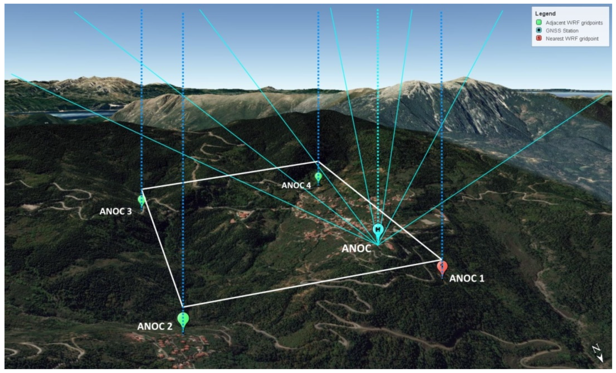
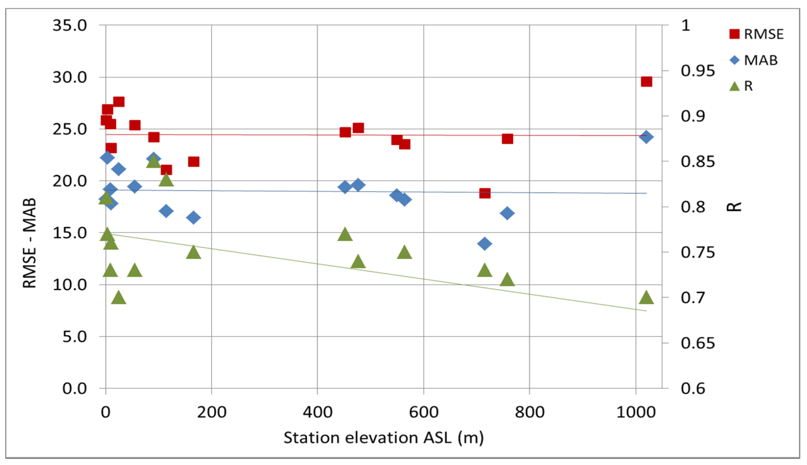
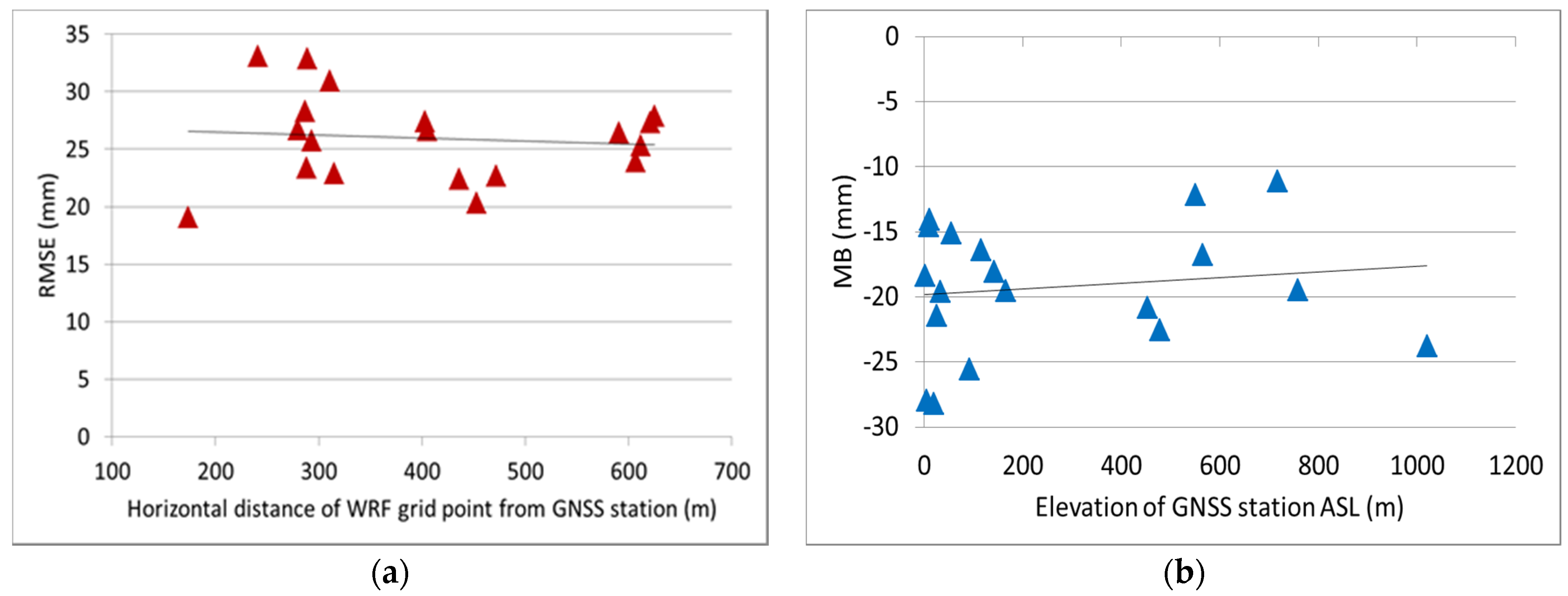
  • As shown in Figure 9a, the RMSE seems to be independent of the horizontal distance s between the GNSS station and the nearest WRF grid point where the calculation of the predicted ZTD is performed. Therefore, we can conclude that the horizontal resolution of 1 km used for the WRF simulation is adequate.
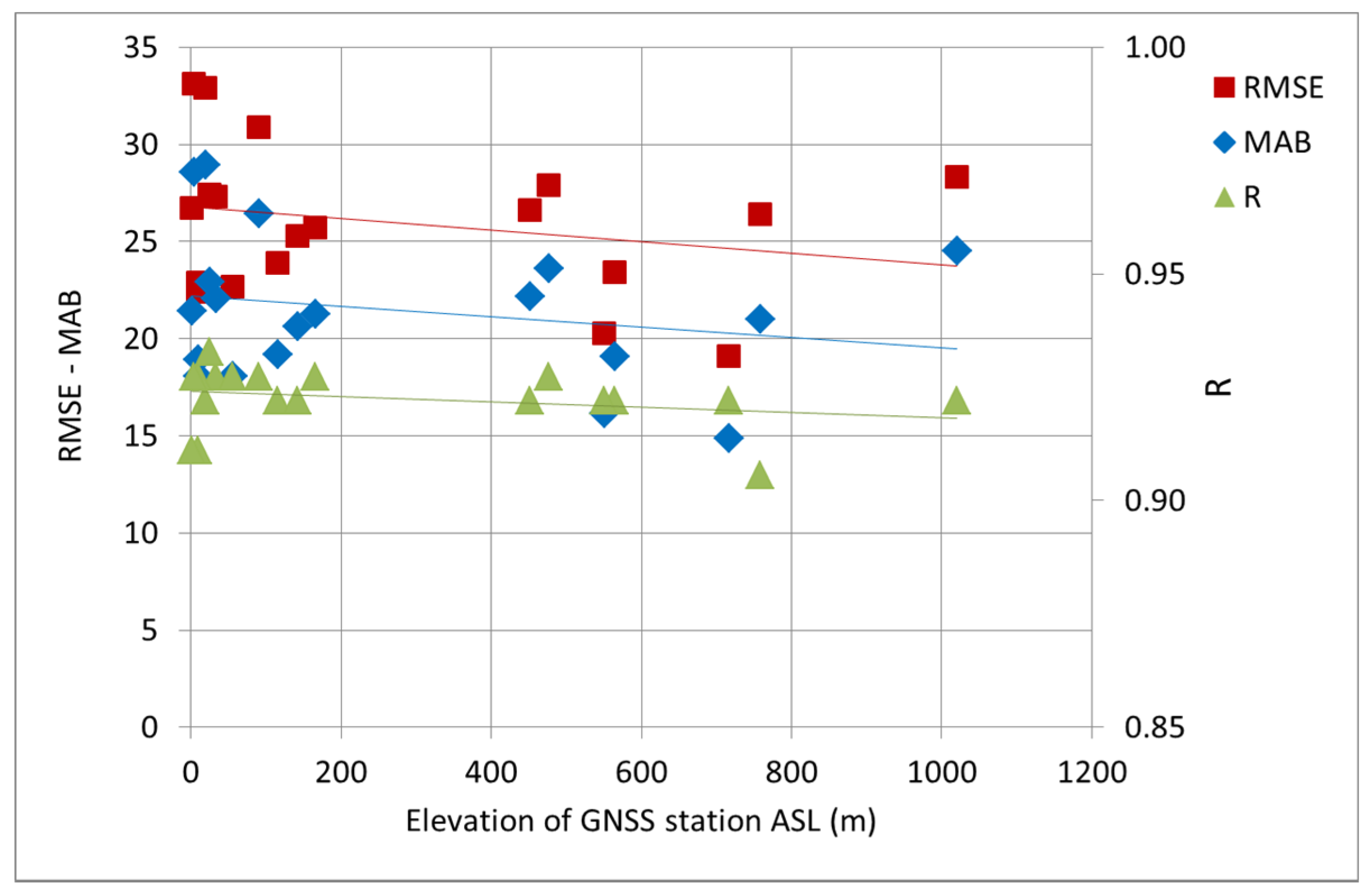
  • With respect to station elevation h, a small reduction of MB in terms of its absolute value is evident with increasing h, as expected, due to smaller ZTD values (Figure 9b). Out of the 19 stations, the three highest mean negative biases are in XILI, PSAT and PAT0 (elevations ASL 4, 19 and 91 m), while the two lowest are in LIDO and KALA (550 and 716 m). The graphical summary of validation metrics for the entire period (Figure 10) also reveals that while R is fairly constant with increasing station elevation, MAB and RMSE exhibit a reduction.

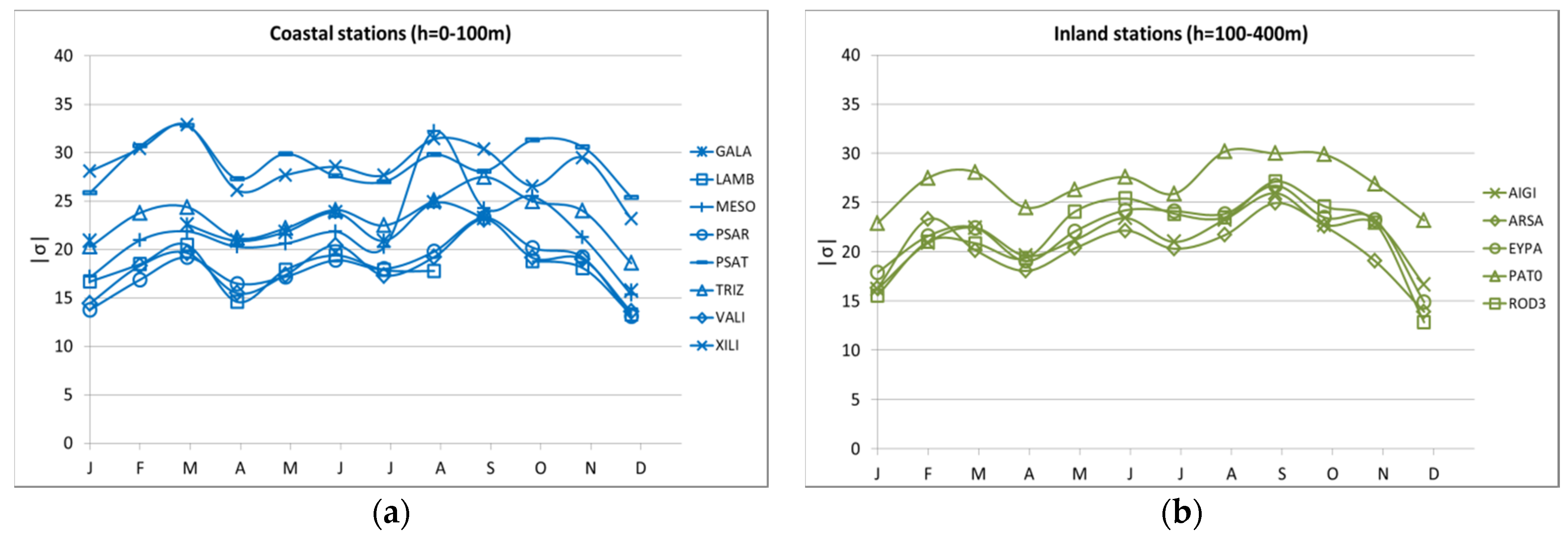
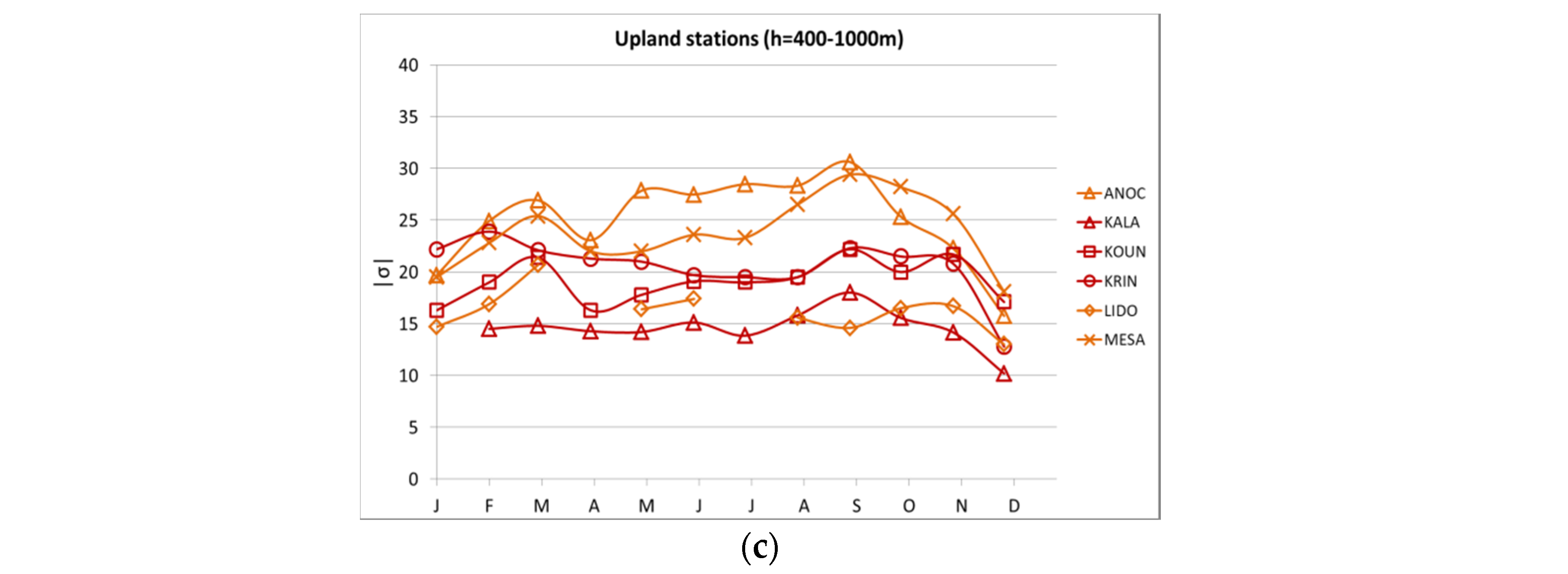
3.3. Seasonal Characteristics of WRF vs. GNSS ZTD and Evaluation of Model Performance

Beyond the annual time series analysis and evaluation, it is useful to perform a more in-depth investigation of seasonal trends, which can provide an important insight into the model’s forecast skill under different meteorological conditions. The year is therefore divided into four seasons (S1-S4) based on their distinct climatological characteristics as follows:
Winter S1: January–March.
Spring S2: April–June.
Summer S3: July–September.
Autumn S4: October–December.
Table 5 lists the corresponding model validation metrics per station and for each season. In general, model performance is better during autumn (S4), as correlation with the observed ZTD time series is high at all stations (R = 0.93 with range 0.91–0.94) and MAB and RMSE are lower (average MAB = 20.5; RMSE = 24.6). In spring (S2), WRF reproduces 88% of the ZTD variability (R = 0.88 with range 0.85–0.89) and exhibits a slightly higher bias than autumn (average MAB = 21.1; RMSE = 25.7). In winter (S1), the model reproduces 85% of the ZTD variability; however, with a wider correlation range between stations (R = 0.85 with range 0.75–0.88), and bias is similar to S2 (average MAB = 21.2; RMSE = 25.2). Model forecasting skill deteriorates during summer (S3), where correlation is weaker (average R = 0.83) and bias indicators are higher (MAB = 22.8, RMSE = 28.0). These results are in-line with seasonal climate characteristics in the region of Western Greece, as stable weather conditions and frontal precipitation patterns which prevail during autumn are well simulated by the model, whereas the combination of high temperatures and turbulent conditions during some summer days, resulting in convective storms are more difficult to predict. A graphical illustration of the RMSE variability for each season, at the location of each station, is seen in Figure 11.
When we look at the monthly variability of the mean absolute bias (Figure 12), a distinct “peak” in February and March is evident in most coastal and inland stations, possibly due to the winter storms which are common during this period. A second “peak” during the summer period (June–September) is explained by a combination of high temperatures and the occurrence of intense convective storm events, as discussed earlier. Stations which are located inland exhibit a more uniform monthly variability of the MAB (co-variance is high), while coastal stations exhibit a more diverse variability, particularly during the “hot” season S3. In stations located upland, two separate groups are distinct: the first one including the Peloponnese stations (south) plus LIDO exhibit a smaller degree of seasonal MAB variability, while ANOC and MESA (both located in the northern Aitoloakarnania region) exhibit higher seasonal variability (distinct “peaks” during S1 and S3 and higher MAB). We can further investigate local inhomogeneities between stations by calculating the correlation coefficient R of their difference, i.e., between the GNSS ΔZTD and WRF ΔZTD of stations MESA and KALA, for seasons S1–S4. Thus, the annual and semi-annual component of ZTD variability is removed from the time series and the ability of the model to resolve small-scale inhomogeneities is demonstrated. Results indicate that model performance is better during the second half of the year, as WRF reproduces 54% of the observed ΔZTD variability between the two stations in summer (S3) and 52% in autumn (S4) (R is 0.54 and 0.52 respectively). The correlation is slightly weaker during the first half, with R = 0.48 in winter (S1) and R = 0.49 in spring (S2).
The overall model performance with respect to estimating the ZTD parameter for the successful tropospheric correction of InSAR interferograms is evaluated by setting the acceptable bias range as the amplitude of one Sentinel-1 C-band cycle phase π (equal to λ/2, where λ is the SAR signal wavelength), i.e., ±23 mm of tropospheric delay, when projected to the zenithal distance (considering a mean incidence angle of 35°). This allows us to determine the percentage of σ lying within the accepted range per season (Table 6), which in theory represents the probability that the model successfully detects and removes the tropospheric delay.

4. Discussion

Results of the physical parameterization analysis indicate that WRF configurations MOD4 and MOD5 overall exhibit a better prediction skill during the test period, with small differences between them. Turning on the Kain–Fritsch cumulus convection scheme on the 9 km domain improves model output, particularly during intense frontal events, as demonstrated by validation metrics of MOD4 in comparison with MOD3 (all physical parameters are the same except the cumulus scheme). Moreover, the use of more complex microphysics schemes (such as Morrison and SBU-YLin), surface layer (Pleim–Xiu and MM5) and planetary boundary layer (ACM2 and YSU) models, although computationally demanding, further enhances the model prediction skill. Indeed, model setup and physical parameterization can affect the intrinsic water balance [44], resulting in a more accurate representation of precipitation and relative humidity fields [25,45]. Based on the results of the parametric analysis, MOD5 is selected as the optimum configuration for producing tropospheric delay maps for the entire PaTrop period (January–December 2016), having a slightly higher R, lower MB and better clustering of RMSE than MOD4.
On an annual basis, the statistical analysis of the results demonstrated that the correlation between predicted and observed ZTDs at the 19 stations is good throughout the year (correlation co-efficient R ranges from 0.91 to 0.93), with mean bias (MB) ranging from −11.1 mm (KALA station) to −28.2 mm (PSAT station), indicating that the model tends to slightly underestimate the tropospheric ZTD as compared to the GNSS derived values. Results are in-line with previous WRF high-resolution studies [25,46,47], which report consistent underestimation of RH at the ground level (ranging from 9 to 15%). With respect to the seasonal component, model performance is better during the autumn period (October–December), followed by the spring period (April–June). Correlation with the observed ZTD time series is high at all stations (correlation co-efficient R is 0.93 and 0.88, respectively) and MAB and RMSE values are low. On the contrary, model forecasting skill seems to deteriorate during summer (July–September), where correlation is weaker (R = 0.83) and MAB and RMSE values are higher (average MAB = 22.8, RMSE = 28.0). Again, results re-confirm research findings from similar comparisons of GNSS tropospheric products and LAMs in Europe [48,49,50], reporting a pronounced seasonal cycle of GNSS-NWP model bias and standard deviation with the largest errors in summer and smallest in winter. Setting the acceptable bias range at ±23 mm (equal to the amplitude of one Sentinel−1 C-band phase cycle when projected to the zenithal distance), it is demonstrated that the model produces satisfactory results, with a percentage of ZTD values within the bias margin ranging from 57% in summer to 63% in autumn.

5. Conclusions

The experimental approach followed aims to maximise the potential of using LAMs for the calculation and removal of the tropospheric noise from InSAR data. Five different WRF parameterization schemes were tested, ranging from schemes with relatively simple physical and dynamical parameterization to more complex schemes which require longer computational times. A parametric analysis was performed for a two-week period (17–29 June 2016), during which the output of different model configurations, in terms of ZTD, was compared with GNSS tropospheric measurements from 16 permanent stations in the study area (d04). Results were tested for their statistical significance and demonstrated that the optimum WRF configuration to be used for the entire period of the PaTrop experiment was MOD5. Consequently, daily runs of the optimal scheme were performed for a one-year period (January–December 2016), and model output was again validated with the use of the observational GNSS dataset from the CRL network in the Western Gulf of Corinth.
Overall, the current study confirms the high potential and effectiveness of using high-resolution atmospheric modelling for calculating the ZTD component, and thus correcting atmospheric phase gradients in interferograms. The innovative elements that our methodology brings in comparison with previous studies are: (a) High-resolution re-analysis with WRF: our model is downscaled at 1 km horizontal resolution and therefore offers a detailed reconstruction of the 3-D tropospheric field over the study area. The model was locally configured and parameterized in the area of the western Gulf of Corinth, and numerous complex schemes were tested in order to demonstrate the optimal configuration at the specific location; (b) Validation of the model: WRF output was validated with the use of GNSS tropospheric data retrieved from a dense array of stations covering the study area. Model validation with vertical column data (GNSS zenithal delays) instead of ground measurements offers the capability of evaluating the model’s forecasting skill over the entire 3-D field, thus enabling fine-tuning of its physical parameterization with the use of a high-accuracy representative observational dataset. This is particularly useful when it comes to estimating the highly variable water vapour signals which are exhibited in the differential atmosphere as densely distributed short-wavelength phase gradients.

Author Contributions

Conceptualization, N.R. and P.B.; methodology, N.R. and P.B.; software, N.R., D.K. and P.B.; validation, N.R.; formal analysis, N.R.; investigation, N.R.; resources, N.R., D.K., P.E. and P.B.; data curation, N.R. and P.B.; writing—original draft preparation, N.R.; writing—review and editing, N.R., P.B., I.K., D.K., P.E., A.A.A. and A.R; visualization, N.R.; supervision, P.B., I.K., A.A.A. and A.R.; project administration, P.B.; funding acquisition, P.B. All authors have read and agreed to the published version of the manuscript.

Funding

This research received no external funding.

Informed Consent Statement

Not applicable.

Data Availability Statement

The data presented in this study are available on request from the corresponding author. The data are not publicly available due to extensive size.

Acknowledgments

This work was supported by computational time granted from the National Infrastructures for Research and Technology S.A. (GRNET S.A.) in the National HPC facility—ARIS—under project IDs PaTrop, PaTrop2 and Atmo-InSAR.

Conflicts of Interest

The authors declare no conflict of interest.

References

  1. Skamarock, W.; Klemp, J.B.; Dudhia, J.; Gill, D.O.; Barker, D.; Duda, M.G.; Huang, X.-Y.; Wang, W. A description of the advanced research WRF version 3. In NCAR Technical Note NCAR/TN-475 + STR; University Corporation for Atmospheric Research: Boulder, CO, USA, 2008. [Google Scholar] [CrossRef]
  2. Foster, J.; Brooks, B.; Cherubini, T.; Shacat, C.; Businger, S.; Werner, C.L. Mitigating atmospheric noise for InSAR using a high resolution weather model. Geophys. Res. Lett. 2006, 33, L16304. [Google Scholar] [CrossRef]
  3. Foster, J.; Kealy, J.; Cherubini, T.; Businger, S.; Lu, Z.; Murphy, M. The utility of atmospheric analyses for the mitigation of artifacts in InSAR. J. Geophys. Res. Solid Earth 2013, 118, 748–758. [Google Scholar] [CrossRef] [Green Version]
  4. Puysségur, B.; Michel, R.; Avouac, J.P. Tropospheric phase delay in interferometric synthetic aperture radar estimated from meteorological model and multispectral imagery. J. Geophys. Res. 2007, 112, B05419. [Google Scholar] [CrossRef] [Green Version]
  5. Wadge, G.; Zhu, M.; Holley, R.; James, I.; Clark, P.; Wang, C.; Woodage, M. Correction of Atmospheric Delay Effects in Radar Interferometry Using a Nested Mesoscale Atmospheric Model. J. Appl. Geophys. 2010, 72, 141–149. [Google Scholar] [CrossRef]
  6. Eff-Darwich, A.; Perez, J.; Fernandez, J.; Garcia-Lorenzo, B. Using a mesoscale meteorological model to reduce the effect of tropospheric water vapour from DInSAR data: A case study for the island of Tenerife. Pure Appl. Geophys. 2012, 169, 1425–1441. [Google Scholar] [CrossRef]
  7. Kinoshita, Y.; Furuya, M.; Hobiger, T.; Ichikawa, R. Are numerical weather model outputs helpful to reduce tropospheric delay signals in InSAR data? J. Geod. 2013, 87, 267–277. [Google Scholar] [CrossRef] [Green Version]
  8. Bekaert, D.P.S.; Walters, R.J.; Wright, T.J.; Hooper, A.; Parker, D.J. Statistical comparison of InSAR tropospheric correction techniques. Remote Sens. Environ. 2015, 170, 40–47. [Google Scholar] [CrossRef] [Green Version]
  9. Delacourt, C.; Briole, P.; Achache, J.A. Tropospheric corrections of SAR interferograms with strong topography. Appl. Etna. Geophys. Res. Lett. 1998, 25, 2849–2852. [Google Scholar] [CrossRef]
  10. Webley, P.W.; Bingley, R.M.; Dodson, A.H.; Wadge, G.; Waugh, S.J.; James, I.N. Atmospheric water vapour correction to InSAR surface motion measurements on mountains: Results from a dense GPS network on Mount Etna. Phys. Chem. Earth 2002, 27, 363–370. [Google Scholar] [CrossRef]
  11. Li, Z.; Muller, J.; Cross, P.; Fielding, E. Interferometric synthetic aperture radar (InSAR) atmospheric correction: GPS, Moderate Resolution Imaging Spectroradiometer (MODIS), and InSAR integration. J. Geophys. Res. 2005, 110. [Google Scholar] [CrossRef]
  12. Löfgren, J.; Björndahl, F.; Moore, A.; Webb, F.; Fielding, E.; Fishbein, E. Tropospheric correction for InSAR using interpolated ECMWF data and GPS Zenith Total Delay from the Southern California Integrated GPS Network. In Proceedings of the 2010 IEEE International Geoscience and Remote Sensing Symposium, Honolulu, HI, USA, 25–30 July 2010; pp. 4503–4506. [Google Scholar] [CrossRef] [Green Version]
  13. Li, Z.; Fielding, E.; Cross, P.; Preusker, R. Advanced InSAR atmospheric correction: MERIS/MODIS combination and stacked water vapour models. Int. J. Remote Sens. 2009, 30, 3343–3363. [Google Scholar] [CrossRef]
  14. Walters, R.; Elliott, J.; Li, Z.; Parsons, B. Rapid strain accumulation on the Ashkabad fault (Turkmenistan) from atmosphere-corrected InSAR. J. Geophys. Res. Atmos. 2013, 118, 1–17. [Google Scholar] [CrossRef] [Green Version]
  15. Xu, W.; Li, Z.; Ding, X.; Feng, G.; Hu, D.; Long, J.; Yin, H.; Yang, E. Correcting atmospheric effects in ASAR interferogram with MERIS integrated water vapor data. Chin. J. Geophys. 2010, 53, 1073–1084. [Google Scholar]
  16. Elliott, J.; Biggs, J.; Parsons, B.; Wright, T. InSAR slip rate determination on the Altyn Tagh Fault, northen Tibet, in the presence of topographically correlated atmopsheric delays. Geophys. Res. Lett. 2008, 35, L12309. [Google Scholar] [CrossRef] [Green Version]
  17. Cavalié, O.; Lasserre, C.; Doin, M.; Peltzer, G.; Sun, J.; Xu, X.; Shen, Z. Measurement of interseismic strain across the Haiyuan fault (Gansu, China) by InSAR. Earth and Plan. Sci. Lett. 2008, 275, 246–257. [Google Scholar] [CrossRef]
  18. Lin, Y.N.; Simons, M.; Hetland, E.A.; Muse, P.; DiCaprio, C.A. Multiscale approach to estimating topographically correlated propagation delays in radar interferograms. Geochem. Geophys. Geosyst. 2010, 11, Q09002. [Google Scholar] [CrossRef]
  19. Doin, M.P.; Lasserre, C.; Peltzer, G.; Cavali, O.; Doubre, C. Corrections of stratified tropospheric delays in SAR interferometry: Validation with global atmospheric models. J. Appl. Geophys. 2009, 69, 35–50. [Google Scholar] [CrossRef]
  20. Jolivet, R.; Grandin, R.; Lasserre, C.; Doin, M.P.; Peltzer, G. Systematic InSAR tropospheric phase delay corrections from global meteorological reanalysis data. Geophys. Res. Lett. 2011, 38, L17311. [Google Scholar] [CrossRef] [Green Version]
  21. Jolivet, R.; Agram, P.S.; Lin, N.Y.; Simons, M.; Doin, M.P.; Peltzer, G.; Li, Z. Improving InSAR geodesy using Global Atmospheric Models. J. Geophys. Res. Solid Earth 2014, 119, 2324–2341. [Google Scholar] [CrossRef]
  22. Yun, Y.; Zeng, Q.; Green, B.W.; Zhang, F. Mitigating atmospheric effects in InSAR measurements through high-resolution data assimilation and numerical simulations with a weather prediction model. Int. J. Remote Sens. 2015, 36, 2129–2147. [Google Scholar] [CrossRef]
  23. Briole, P.; Rigo, A.; Lyon-Caen, H.; Ruegg, J.C.; Papazissi, K.; Mitsakaki, C.; Balodimou, A.; Veis, G.; Hatzfeld, D.; Deschamps, A. Results from repeated Global Positioning System surveys between 1990 and 1995. J. Geophys. Res. 2000, 105, 25605–25625. [Google Scholar] [CrossRef] [Green Version]
  24. Avallone, A.; Briole, P.; Agatza-Balodimou, A.M.; Billiris, H.; Charade, O.; Mitsakaki, C.; Nercessian, A.; Papazissi, K.; Paradissis, D.; Veis, G. Analysis of eleven years of deformation measured by GPS in the Corinth Rift Laboratory area. C.R. Geosci. 2004, 336, 301–312. [Google Scholar] [CrossRef] [Green Version]
  25. Kioutsioukis, I.; De Meij, A.; Jakobs, H.; Katragkou, E.; Vinuesa, J.F.; Kazantzidis, A. High resolution WRF ensemble forecasting for irrigation: Multi-variable evaluation. Atmos. Res. 2015, 167, 156–174. [Google Scholar] [CrossRef]
  26. Garcia-Diez, M.; Fermandez, J.; Vautard, R. An RCM multi-physics ensemble over Europe: Multi-variable evaluation to avoid error compensation. Clim. Dyn. 2015, 45, 3141–3156. [Google Scholar] [CrossRef] [Green Version]
  27. Bevis, M.; Businger, S.; Herring, T.; Rocken, C.; Anthes, R.; Ware, R. GPS meteorology: Remote sensing of atmospheric water vapor using the global positioning system. J. Geophys. Res. 1992, 97, 15787–15801. [Google Scholar] [CrossRef]
  28. Elgered, G.; Davis, J.L.; Herring, T.A.; Shapiro, I.I. Geodesy by radio interferometry: Water vapor radiometry for estimation of the wet delay. J. Geophys. Res. 1991, 96, 6541–6555. [Google Scholar] [CrossRef]
  29. Davis, J.L.; Herring, T.A.; Shapiro, I.I.; Rogers, A.E.; Elgered, G. Geodesy by radio interferometry: Effects of atmospheric modeling errors on estimates of baseline length. Radio Sci. 1985, 20, 1593–1607. [Google Scholar] [CrossRef]
  30. Mooney, P.A.; Mulligan, F.J.; Fealy, R. Evaluation of the sensitivity of the weather research and forecasting model to parameterization schemes for regional climates of Europe over the period 1990–95. J. Clim. 2013, 26, 1002–1017. [Google Scholar] [CrossRef] [Green Version]
  31. Kotlarski, S.; Keuler, K.; Christensen, O.B.; Colette, A.; Déqué, M.; Gobiet, A.; Goergen, K.; Jacob, D.; Lüthi, D.; van Meijgaard, E.; et al. Regional climate modeling on European scales: A joint standard evaluation of the EURO-CORDEX RCM ensemble. Geosci. Model Dev. 2014, 7, 1297–1333. [Google Scholar] [CrossRef] [Green Version]
  32. Garcia-Diez, M.; Fernandez, J.; Fita, L.; Yague, C. Seasonal dependence of WRF model biases and sensitivity to PBL schemes over Europe. Q. J. R. Meteorol. Soc. 2013, 139, 501–514. [Google Scholar] [CrossRef] [Green Version]
  33. Kain, J.S.; Fritsch, M. A one-dimensional entraining/detraining plume model and its application in convective parameterization. J. Atmos. Sci. 1990, 47, 2784–2802. [Google Scholar] [CrossRef] [Green Version]
  34. Kain, J.S. The Kain–Fritsch convective parameterization: An update. J. Appl. Meteorol. 2004, 43, 170–181. [Google Scholar] [CrossRef] [Green Version]
  35. Zheng, Y.; Alapaty, K.; Herwehe, J.; Delgenio, A.; Niyogi, D. Improving high-resolution weather forecasts using the weather research and forecasting (WRF) model with an updated Kain–Fritsch scheme. Mon. Weather Rev. 2015, 144, 150528113541009. [Google Scholar] [CrossRef]
  36. Mlawer, E.J.; Taubman, S.J.; Brown, P.D.; Iacono, M.J.; Clough, S.A. Radiative transfer for inhomogeneous atmospheres: RRTM, a validated correlated-k model for the longwave. J. Geophys. Res. 1997, 102, 16663–16682. [Google Scholar] [CrossRef] [Green Version]
  37. Dudhia, J. Numerical study of convection observed during the winter monsoon experiment using a mesoscale two-dimensional model. J. Atmos. Sci. 1989, 46, 3077–3107. [Google Scholar] [CrossRef]
  38. Morrison, H.; Thompson, G.; Tatarskii, V. Impact of cloud microphysics on the development of trailing stratiform precipitation in a simulated squall line: Comparison of one- and two-moment schemes. Mon. Weather Rev. 2009, 137, 991–1007. [Google Scholar] [CrossRef] [Green Version]
  39. Warrach-Sagi, K.; Schwitalla, T.; Wulfmeyer, V.; Bauer, H. Evaluation of a climate simulation in Europe based on the WRF–NOAH model system: Precipitation in Germany. Clim. Dyn. 2013, 41, 755–774. [Google Scholar] [CrossRef] [Green Version]
  40. Pleim, J.E.; Xiu, A. Development and testing of a surface flux and planetary boundary layer model for application in mesoscale models. J. Appl. Meteor. 1995, 34, 16–32. [Google Scholar] [CrossRef] [Green Version]
  41. Xiu, A.; Pleim, J.E. Development of a land surface model part I: Application in a mesoscale meteorology model. J. Appl. Meteor. 2001, 40, 192–209. [Google Scholar] [CrossRef]
  42. Zhang, C.; Lin, H.; Chen, M.; Yang, L. Scale matching of multiscale digital elevation model (DEM) data and the Weather Research and Forecasting (WRF) model: A case study of meteorological simulation in Hong Kong. Arab J. Geosci. 2014, 7, 2215–2223. [Google Scholar] [CrossRef]
  43. Lin, Y.; Colle, B.A. A new bulk microphysical scheme that includes riming intensity and temperature-dependent ice characteristics. Mon. Weather Rev. 2011, 139, 1013–1035. [Google Scholar] [CrossRef]
  44. Fersch, B.; Kunstmann, H. Atmospheric and terrestrial water budgets: Sensitivity and performance of configurations and global driving data for long term continental scale WRF simulations. Clim. Dyn. 2014, 42, 2367–2396. [Google Scholar] [CrossRef] [Green Version]
  45. Madala, S.; Satyanarayana, A.; Srinivas, C.; Bhishma, T. Performance evaluation of PBL schemes of ARW model in simulating thermo-dynamical structure of pre-monsoon convective episodes over Kharagpur using STORM data sets. Pure Appl. Geophys. 2016, 173, 1803–1827. [Google Scholar] [CrossRef]
  46. Schwitalla, T.; Bauer, H.-S.; Wulfmeyer, V.; Aoshima, F. High resolution simulation over central Europe: Assimilation experiments during COPS IOP 9c. Q. J. Roy. Meteor. Soc. 2011, 137, 156–175. [Google Scholar] [CrossRef]
  47. Politi, N.; Nastos, P.T.; Sfetsos, A.; Vlachogiannis, D.; Dalezios, N.R. Evaluation of the AWR-WRF model configuration at high resolution over the domain of Greece. Atmos. Res. 2018, 208, 229–245. [Google Scholar] [CrossRef]
  48. Guerova, G.; Brockmann, E.; Quiby, J.; Schubiger, F.; Matzler, C. Validation of NWP mesoscale models with Swiss GPS Network AGNES. J. App. Meteorol. 2003, 42, 141–150. [Google Scholar] [CrossRef]
  49. Guerova, G.; Brockmann, E.; Schubiger, F.; Morland, J.; Matzler, C. An integrated assessment of measured and modeled IWV in Switzerland for the period 2001–2003. J. App. Meteorol. 2005, 44, 1033–1044. [Google Scholar] [CrossRef]
  50. Haase, J.; Ge, M.; Vedel, H.; Calais, E. Accuracy and variability of GPS tropospheric delay measurements of water vapor in the western Mediterranean. J. App. Meteorol. 2003, 42, 1547–1568. [Google Scholar] [CrossRef]
Figure 1. (a) Left, map showing the four nested domains (d01-d04) used for WRF weather re-analysis over the Western GoC. (b) Right, map of the PaTrop study area, Western GoC. Previously installed permanent GNSS stations are marked in blue colour, newly installed GNSS stations marked in red colour. The black box indicates the location of the 1 × 1 km inner domain of the WRF re-analysis run (Domain d04).
Remotesensing 13 01898 g001
Figure 2. Example of GNSS-WRF geometry for ANOC Station (h = 1020 m). Dark blue dotted lines depict the ZTD path calculated by WRF at the four nearest grid points, light blue lines depict the GNSS slant paths measured by the receiver at the time of acquisition and light blue dotted line depicts the ZTD path calculated by the GIPSY tropospheric processing.
Remotesensing 13 01898 g002
Figure 3. Observed and simulated time series of WRF MOD1-MOD5 vs. GNSS ZTDs at 4 PaTrop stations, KALA (a), MESA (b), EYPA (c) and PSAR (d) over the test period (17–29 June 2016).
Remotesensing 13 01898 g003
Figure 4. Bias plots of predicted (WRF MOD5) minus observed (GNSS) ZTDs at 4 PaTrop stations, KALA (a), MESA (b), EYPA (c) and PSAR (d) over the test period (17–29 June 2016). The red line indicates the mean bias.
Remotesensing 13 01898 g004
Figure 5. RMSE distribution at the 16 stations, for each model configuration. Stations are colour-coded, according to their location: blue—coastal; green—inland; orange—upland north; red—upland south.
Remotesensing 13 01898 g005
Figure 6. Distribution of model validation metrics (MAB, RMSE and PPC) per station elevation h—MOD5.
Remotesensing 13 01898 g006
Figure 7. Observed and simulated time series of WRF MOD5 vs. GNSS ZTDs at 4 PaTrop stations, KALA (a), MESA (b), EYPA (c) and PSAR (d) over January–December 2016.
Remotesensing 13 01898 g007
Figure 8. Bias plots of predicted (WRF MOD5) minus observed (GNSS) ZTDs at 4 PaTrop stations, KALA (a), MESA (b), EYPA (c) and PSAR (d) over January–December 2016. The yellow line indicates the mean bias (MB).
Remotesensing 13 01898 g008
Figure 9. Plots of: RMSE vs. horizontal distances between WRF grid point and GNSS station (a); MB vs. GNSS station elevation h (b).
Remotesensing 13 01898 g009
Figure 10. Distribution of model validation metrics (MAB, RMSE and R) per station elevation h.
Remotesensing 13 01898 g010
Figure 11. RMSE per station and season (S1 top left, S2 top right, S3 bottom left, S4 bottom right).
Remotesensing 13 01898 g011aRemotesensing 13 01898 g011b
Figure 12. Monthly variability of MAB at the 19 PaTrop stations, classified per terrain type: coastal (a); inland (b); upland (red = north, orange = south) (c).
Remotesensing 13 01898 g012aRemotesensing 13 01898 g012b
Table 1. CRL tropospheric solution settings—all stations.
SoftwareGipsy 6.4
GNSSGPS and GLONASS
Troposphere estimated parametersZTD (5 min)
IonosphereHOI included
Ocean tidesFES2004
ZTD timestamphh:00 and hh:30
Elevation cut-off5
Table 2. WRF parameterization options used for the PaTrop sensitivity analysis.
MOD1MOD2MOD3MOD4MOD5
Microphysics (mp)WSM3 Morrison MorrisonMorrisonSBU-YLin
Land surface (sf)NOAH NOAH Pleim-XiuPleim-XiuNOAH
Surface layer physics (sfclay)Monin-Obukhov Monin-Obukhov Pleim-XiuPleim-XiuMM5 similarity
Radiation physics (sw)Dudhia Dudhia DudhiaDudhiaDudhia
Radiation physics (lw)RRTM RRTM RRTMRRTMRRTM
Planetary boundary layer physics (pbl)MYJ MYJ ACM2ACM2YSU
Cloud physics (cu)Kain-Fritsch at 27 kmKain-Fritsch at 27 kmKain-Fritsch at 27 kmKain-Fritsch
at 27 and 9 km
Kain-Fritsch
at 27 and 9 km
Table 3. Pearson Correlation Co-efficient and RMSE results for all schemes (17/6–29/6/2016).
StationElevation (m)RRMSE (mm)
MOD1MOD2MOD3MOD4MOD5MOD1MOD2MOD3MOD4MOD5
MESO20.730.740.780.770.8130.530.928.326.125.1
XILI40.700.710.760.780.7732.432.630.326.626.7
VALI90.700.680.700.710.7325.226.425.424.424.4
LAMB100.700.710.740.750.7625.225.423.122.822.9
TRIZ250.630.610.700.700.7027.028.426.624.824.9
PSAR550.690.680.750.730.7326.728.026.424.123.1
PAT0910.770.780.810.840.8529.930.525.024.627.6
ARSA1150.740.750.790.820.8327.027.523.022.123.3
EYPA1660.670.680.740.750.7527.327.624.722.822.8
ROD34520.710.710.740.760.7728.428.926.724.826.7
MESA4770.670.690.740.740.7428.528.927.325.425.1
LIDO5500.600.600.670.600.5729.830.029.528.026.6
KOUN5640.710.690.710.730.7525.727.025.023.523.1
KALA7160.660.660.690.700.7322.322.620.120.621.4
KRIN7580.680.660.670.700.7222.824.523.021.722.2
ANOC10200.660.670.720.720.7035.536.535.132.231.4
AVG160.690.690.730.730.7427.828.526.224.624.4
Table 4. Statistical indices of complete WRF ZTS vs. GNSS ZTD time series—January–December 2016.
StationElevation ASL (m)ΜΒΜΑΒRMSER
ANOC 1020−23.824.528.30.92
ARSA 115−16.419.223.90.92
AIGI 142−18.120.725.30.92
GALA 33−19.622.127.30.93
EYPA 166−19.521.325.70.93
KALA 716−11.114.919.10.92
KOUN 564−16.819.123.40.92
KRIN 758−19.421.026.40.91
LAMB 10−14.019.022.40.91
LIDO 550−12.116.120.30.92
MESA 477−22.523.727.90.93
MESO 2−18.321.426.70.91
PAT091−25.526.530.90.93
PSAR 55−15.118.122.70.93
PSAT 19−28.229.032.90.92
ROD3 452−20.822.226.50.92
TRIZ 25−21.422.927.40.93
VALI 9−14.518.122.90.93
XILI 4−28.028.633.10.93
AVG19 −19.221.525.90.92
Table 5. Seasonal statistical indices of WRF ZTS vs. GNSS ZTD time series—2016.
Season S1 S2 S3 S4
|σ|RMSER|σ|RMSER|σ|RMSER|σ|RMSER
ANOC 24.928.00.8525.128.90.8925.830.50.8222.325.60.93
ARSA 19.824.20.8618.322.80.8920.625.80.8418.122.40.93
AIGI 19.623.50.8120.425.20.8922.227.60.8420.824.60.93
GALA 22.127.10.8422.327.40.8723.128.60.86---
EYPA 20.924.60.8720.324.90.8922.927.90.8421.125.00.94
KALA 14.218.30.8215.019.00.8916.721.50.8313.417.00.93
KOUN 18.922.60.8317.722.00.8920.225.40.8419.623.40.93
KRIN 22.727.90.7520.726.60.8720.425.70.8218.323.30.91
LAMB 18.522.80.8417.522.40.8718.423.10.8416.621.40.93
LIDO 16.820.60.8816.520.90.8516.221.10.8515.519.20.93
MESA 22.526.00.8722.626.80.8826.331.00.8223.127.10.93
MESO 20.023.90.8820.925.20.8925.332.20.7120.324.90.94
PAT026.029.40.8826.130.40.8828.633.10.8226.430.40.93
PSAR 16.921.00.8517.822.40.8920.325.50.8517.321.60.94
PSAT 30.133.20.8628.232.60.8728.033.10.8429.132.80.94
ROD3 19.323.80.8423.327.40.8924.629.30.8521.626.40.92
TRIZ 22.526.40.8722.827.20.8924.930.20.8422.526.50.94
VALI 17.521.70.8417.822.80.8920.025.50.8417.221.50.94
XILI 30.533.60.8627.532.70.8829.835.00.8426.330.60.94
AVG1921.225.20.8521.125.70.8822.828.00.8320.524.60.93
Table 6. σ values within error range—WRF vs. GNSS ZTDs average of all stations.
SeasonRatio of σ above
π (23 mm)
Ratio of σ below
–π (−23 mm)
Ratio of σ between
π and π
S1<0.010.390.61
S20.010.370.62
S3 0.020.410.57
S4<0.010.370.63
Publisher’s Note: MDPI stays neutral with regard to jurisdictional claims in published maps and institutional affiliations.

