
Mapping Impervious Surface Areas Using Time-Series Nighttime Light and MODIS Imagery


1
School of Remote Sensing and Information Engineering, Wuhan University, Wuhan 430079, China
2
Department of Geosciences, University of Arkansas, Fayetteville, AR 72701, USA
*
Author to whom correspondence should be addressed.
Remote Sens. 2021, 13(10), 1900; https://0-doi-org.brum.beds.ac.uk/10.3390/rs13101900
Submission received: 28 March 2021
/
Revised: 7 May 2021
/
Accepted: 9 May 2021
/
Published: 13 May 2021
Abstract
:Mapping impervious surface area (ISA) dynamics at the regional and global scales is an important task that supports the management of the urban environment and urban ecological systems. In this study, we aimed to develop a new method for ISA percentage (ISA%) mapping using Nighttime Light (NTL) and MODIS products. The proposed method consists of three major steps. First, we calculated the Enhanced Vegetation Index (EVI)-adjusted NTL index (EANTLI) and performed intra-annual and inter-annual corrections on the DMSP-OLS data. Second, based on the geographically weighted regression (GWR) model, we built a consistent NTL product from 2000 to 2019 by performing an intercalibration between DMSP-OLS and VIIRS images. Third, we adopted a GA-BP neural network model to monitor ISA% dynamics using NTL imagery, MODIS imagery, and population data. Taking the Guangdong–Hong Kong–Macao Greater Bay as the study area, our results indicate that the ISA% in our study area increased from 7.97% in 2000 to 17.11% in 2019, with a mean absolute error (MAE) of 0.0647, root mean square error (RMSE) of 0.1003, Pearson’s coefficient of 0.9613, and R2 (R-squared) of 0.9239. Specifically, these results demonstrate the effectiveness of the proposed method in mapping ISA and investigating ISA dynamics using temporal features extracted from consistent NTL and MODIS products. The proposed method is feasible when generating ISA% at a large scale at high frequency, given the ease of implementation and the availability of input data sources.

1. Introduction
The world has experienced rapid urbanization in the past decades. As of 2014, more than 54% of the global population resided in urban areas, and by 2050, 66% of the world’s population are expected to be living in urban areas [1]. The rapid growth of urban population and economic activities indicate that China is experiencing the largest mass urbanization in human history [2,3]: the percent of the urban population having increased from 11.18% in 1950 to 36.22% in 2000 and to 60.6% in 2019 [4]. Such a rapid urbanization process has caused enormous impacts on urban climate [5,6,7], plant phenology [8,9], habitat dynamics [10], biogeochemical cycles [11], and hydrological patterns [12,13,14]. Therefore, long-term urban expansion monitoring is necessary for sustainable urban development. Impervious surfaces have been recognized as the most direct embodiment of urbanization, a key attribute that can represent urban environmental quality and is one of the predominant indicators of human settlements. Hence, numerous studies have been conducted to characterize impervious surface distributions with an array of remote sensing based methods that vary at the global, continental, national, regional, and city scales [15,16,17,18,19,20]. The authors of [21,22,23] provided overviews of the methods that estimate impervious surfaces using remote sensing imagery.
A better understanding of impervious surface dynamics contributes to the knowledge of the urbanization process and its potential influence on the urban ecological environment. For instance, Powell et al. [24] documented impervious surface changes over 34 years in the Snohomish Water Resource Inventory Area. Their study demonstrated the value of constructing long-term remote sensing time-series images for monitoring impervious surface dynamics. Sexton et al. [25] extracted annual impervious surface coverages over 27 years (1984–2010) in Washington, D.C.–Baltimore, MD megalopolis from the Landsat archive. Shao et al. [16] proposed a model designed to monitor large-scale impervious surfaces using the Defence Meteorological Satellite Program’s Operational Linescan System (DMSP-OLS) images and built impervious surface fraction maps of the Yangtze River Delta from 2000 to 2009. Targeting the Pearl Rivel Delta, China, Zhang et al. [26,27] estimated impervious surfaces by identifying temporal-spectral differences between impervious and pervious surfaces from dense time series Landsat imagery. Gong et al. [28] mapped annual Global Artificial Impervious Areas (GAIA) for a 34-year period (1985–2018) using Landsat, Nighttime Light (NTL), and Sentinel-1 Synthetic Aperture Radar data. With the advent of NTL data, NTL intensity has been widely adopted as an accordant proxy for impervious surface mapping.
In NTL studies, data from the DMSP-OLS and from the Suomi National Polar-orbiting Partnership satellite’s Visible Infrared Imaging Radiometer Suite (NPP-VIIRS) are the most common NTL sources given their long temporal coverage. DMSP-OLS archives data from 1992 to 2013 on a yearly basis, while NPP-VIIRS started to capture NTL intensity in 2012. These two NTL data sources have been widely used for analyzing urbanization processes [29,30,31], estimating socioeconomic parameters [10,32,33,34], and evaluating armed conflicts [35,36]. Many impervious surface mapping methods using NTL data have been proposed [37,38,39,40], among which the thresholding approach has been adopted by many researchers [41,42]. However, the thresholding approach was not effective, as no single optimal threshold can well delineate cities with different sizes [39,43]. In addition, optimal thresholds vary across spatial and temporal domains. Thus, mapping impervious surfaces at a large spatiotemporal scale requires a scheme for dynamic thresholds [44,45,46]. Zhou et al. [45] developed a cluster-based method using DMSP/OLS NTL data to estimate optimal thresholds and map urban extents in both the United States and China. Li et al. [46] proposed an optimal threshold scheme using a vegetation adjusted NTL urban index and the percentage impervious surface area to extract urban areas within seven Southeastern U.S. states. Xie et al. [47] proposed an object-based method for NTL image data and determined the optimal thresholds by comparing reference- and target-year thresholds.
However, DMSP-OLS images are subject to several intrinsic limitations. For instance, the lack of on-orbit radiometric calibration, data saturation, and blooming tends to result in the overestimation of impervious surfaces in urban-suburban areas [48]. To improve the accuracy of impervious surface mapping at the regional and global scales, researchers started to use machine learning models and develop spectral indices to integrating NTL data with auxiliary data, e.g., the Moderate Resolution Imaging Spectroradiometer (MODIS), volunteered geographical information, gridded population data, and social sensing data. Lu et al. [39] developed a Human Settlement Index (HSI) by combining the DMSP-OLS and the MODIS Normalized Difference Vegetation Index (NDVI) data, thus overcoming the omission of the impervious surface areas in a small proportion of settlements, such as towns and villages. Zhang et al. [49] combined MODIS NDVI with NTL to build a vegetation-adjusted NTL urban index (VANUI) that reduces the effect of NTL saturation and increases the variation of the NTL data. Guo et al. [50] presented a normalized impervious surface index (NISI) that integrates DMSP-OLS with MODIS NDVI to map the ISA% distribution of ten metropolitan areas in China via a support vector regression approach. Cao et al. [51] proposed a percolation-based method to extract the urban areas of 28 countries by integrating a variety of data sources that include population, road, and NTL data.
Compared with the intrinsic limitations of DMSP-OLS sensors, however, the inconsistency between DMSP-OLS and VIIRS is more challenging. A cross-sensor calibration model must be established for different NTL images to obtain consistent NTL time series data. Li et al. [52] used the VIIRS and DMSP-OLS archives to build a power function model that generates VIIRS-like DMSP-OLS data. Zheng et al. [53] developed a geographically weighted regression model (GWRc) for NTL data cross-sensor calibration.
In this study, we propose a novel approach to map the dynamics of ISA% from multisource data, including DMSP-OLS and VIIRS NTL composite data, MODIS products, and population data. Specifically, the objectives of this study are summarized below:
- (1)
- We adopted the Enhanced Vegetation Index (EVI)-adjusted NTL index (EANTLI) to mitigate saturation and blooming in DMSP-OLS imagery, improve the light intensity variations and spatial details in urban cores, and reduce the overestimation of impervious surfaces in suburban areas.
- (2)
- We adopted Seasonal and Trend decomposition using Loess (STL) to decompose monthly VIIRS NTL data and estimate annual VIIRS NTL composites to match the temporal resolution of DMSP-OLS data.
- (3)
- We built a cross-sensor calibration model to generate consistent NTL time series data by combining EANTLI and annual VIIRS NTL images.
- (4)
- We developed a multisource-driven ISA% estimation model for impervious surface mapping.
2. Materials and Methods
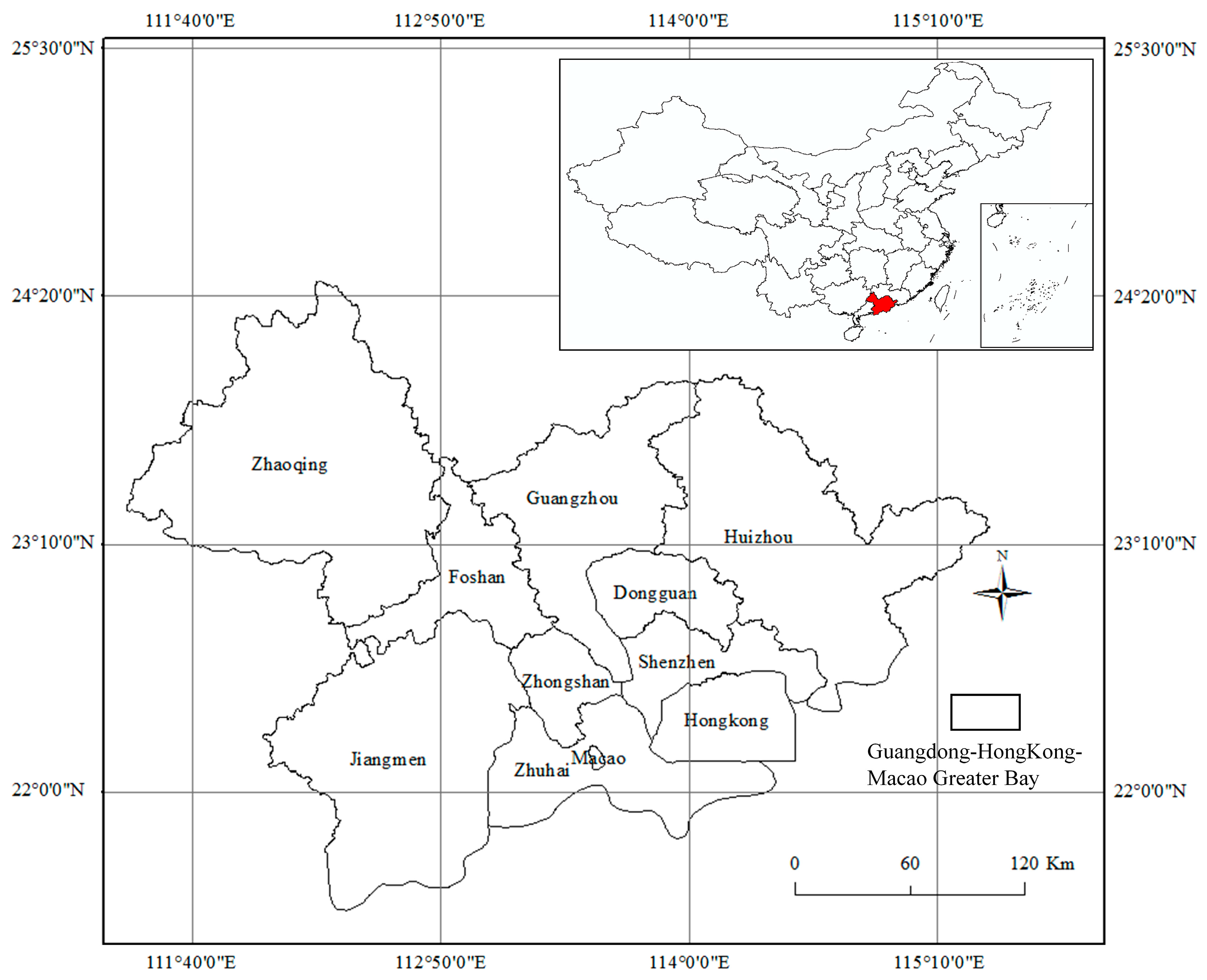
To evaluate the performance of our proposed model, we took Guangdong–Hong Kong–Macao Greater Bay (Figure 1) as a study case. Located in southern China, the geographic location of Guangdong–Hong Kong–Macao Greater Bay is between 111°12′ E–115°35′ E and 21°25′ N–24°30′ N, with a total population of 70 million in 2017. The Greater Bay contains the Pearl River Delta, the largest urban agglomeration in the world, and two special administrative regions of Hong Kong and Macao. The study area is one of the most open and economically dynamic regions in China. Given its rapid growth, this area experienced a long period of unbalanced internal development [54], evidenced by its notably heterogeneous spatial urbanization patterns and distribution of impervious surfaces.
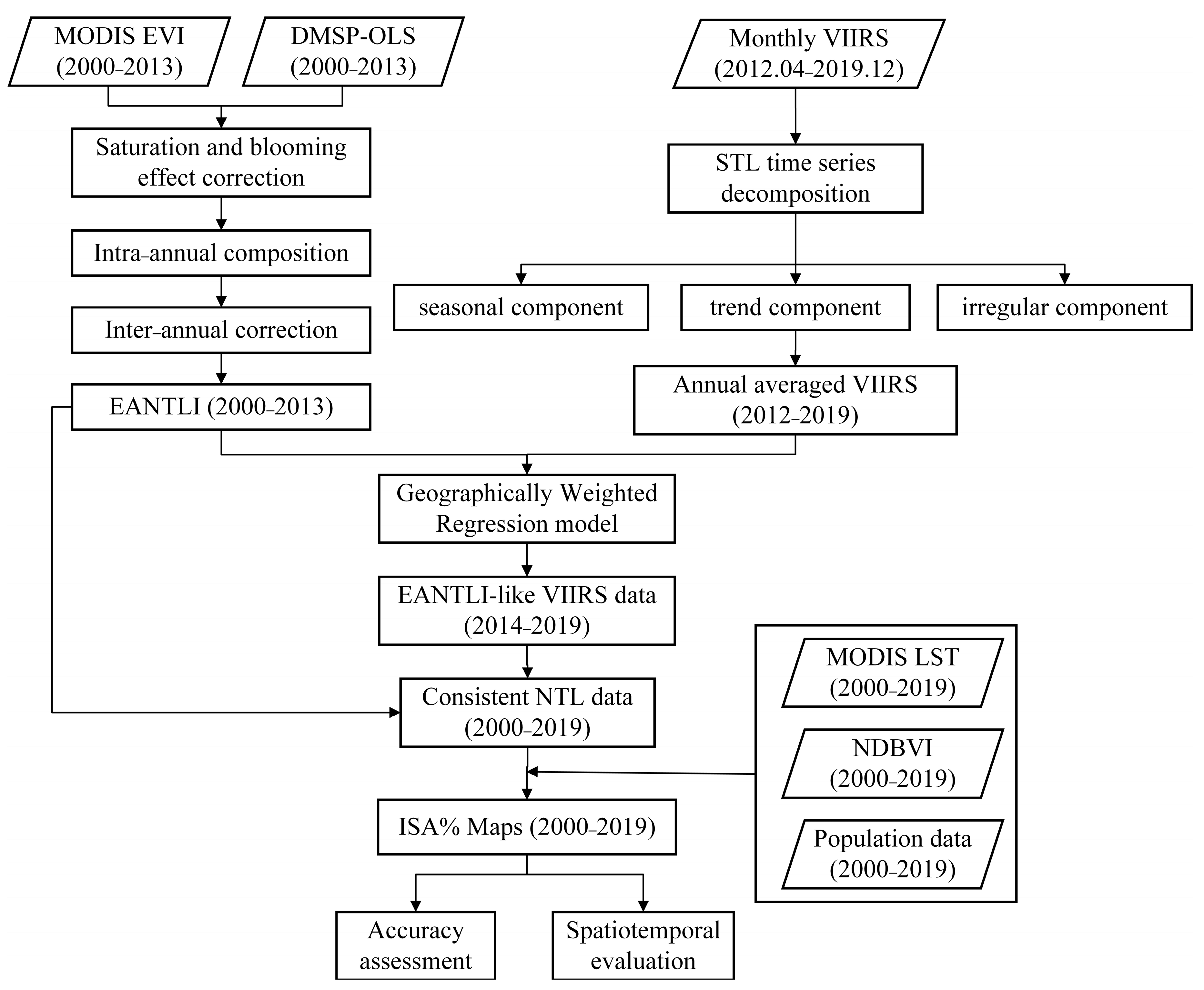
Figure 2 shows the workflow of the proposed ISA% mapping model. In this study, we used three datasets: NTL, MODIS, and population data. These datasets capture three urban elements: economic activity, ecology, and population. The MODIS EVI data and DMSP-OLS data from 2000 to 2013 were used to calculate EANTLI. Intra-annual and inter-annual corrections were performed to improve the performance of EANTLI. In addition, we utilized the STL algorithm to decompose the monthly VIIRS NTL images and calculate the annual VIIRS NTL values. We adopted a GWR model for intercalibration of the EANTLI and VIIRS NTL data, and utilized the consistent NTL data, Land Surface Temperature (LST), Improved Normalized Difference Built-up Index (NDBVI), and population data for ISA% mapping.
2.1. Materials
2.1.1. NTL Data
The NTL data we used included DMSP-OLS and NPP-VIIRS images. The Version-4 DMSP-OLS NTL data set contains cloud-free annual composites collected from 1992 to 2013, covering an area from 180° E to 180° W and 65° S to 75° N. The 34 annual NTL images over a 22-year period are all in the 30 arc-second grids (approximately 1 km at the equator), with DN values ranging from 0 to 63. The DMSP/OLS NTL products we used are the version 4 “stable lights” series compiled over a 22-year span (1992–2013). The version 4 DMSP/OLS stable lights product already excludes sunlight, glare, moonlight, cloud coverage, and lighting [55,56], as well as ephemeral events such as wildfires. In this study, we retrieved the DMSP-OLS NTL dataset with a temporal coverage from 2000 to 2013.
The NPP-VIIRS NTL data, with mitigated saturation and blooming issues, was produced from the Visible Infrared Imaging Radiometer Suite (VIIRS) Day/Night Band (DNB) [57]. We used the Version 1 monthly composite VIIRS data with a 15 arc-second spatial resolution and a temporal coverage from April 2012 to December 2019. VIIRS DNB and DMSP-OLS Nighttime Light products were retrieved from the Earth Observation Group, Payne Institute for Public Policy, Colorado School of Mines (https://eogdata.mines.edu/products/dmsp/ (accessed on 8 September 2020); https://eogdata.mines.edu/products/vnl/ (accessed on 10 September 2020).
2.1.2. MODIS Data
The MODIS data that we used in this study contained Enhanced Vegetation Index (EVI), Normalized Difference Vegetation Index (NDVI), Land Surface Temperature (LST), and the surface spectral reflectance of Terra MODIS Bands 2 and 6. The MOD11A2 products include average LST values under clear-sky during an 8-day period and are stored on a Sinusoidal grid at a spatial resolution of 1 km. We averaged the 8-days period LST values per pixel for the whole year to derive an annual composite LST value. The MOD13A3 product provides monthly EVI and monthly NDVI data with a spatial resolution of 1 km in a Sinusoidal projection. The EVI is an improvement on traditional NDVI, as EVI avoids the saturation problem found in the NDVI for high vegetation coverage areas and considers the influence of the soil background on vegetation index. Moreover, the EVI uses the blue band to remove residual atmosphere contamination caused by smoke and thin clouds. We derived the annual average EVI and annual average NDVI to further mitigate the sensitivity to seasonal and inter-annual fluctuations. We used the annual average EVI and DMSP-OLS to calculate the EANTLI to mitigate saturation and blooming in the DMSP-OLS data. The MOD09A1 product provides an estimation of the surface spectral reflectance corrected for atmospheric conditions in the Terra MODIS Bands 1 through 7. The value of each pixel is selected from all the acquisitions within the 8-day composite period at a spatial resolution of 500 m.
The Normalized Difference Built-up Index (NDBI) is calculated as the reflectance ratio of short-wave infrared band and near-infrared band. Its improved version, the Improved Normalized Difference Built-up Index (NDBVI), outperforms the original NDBI in mapping urban land-use areas [58]. NDBI can be calculated using the following equation:
where RSWIR and RNIR are the surface reflectance of the short wave infrared band (Band 6) and near-infrared band (Band 2) derived from the MOD09A1 product, respectively.
where NDBIavg describes the average annual NDBI derived from Equation (1), NDVIavg represents the annual average NDVI derived from MOD13A3 monthly NDVI product.
MODIS data were downloaded from https://ladsweb.modaps.eosdis.nasa.gov/ (accessed on 28 September 2020), reprojected to the WGS 1984 geographic coordinate system, and resampled to the same cell size as the NTL data.
2.1.3. Population Data
The population data were downloaded in Geotiff format at a resolution of 30 arc-second (approximately 1 km at the equator) in the WGS 1984 geographic coordinate system from the WorldPop (https://www.worldpop.org (accessed on 15 October 2020). WorldPop, collaborating with many national statistical offices and ministries of health, was initiated in 2011. These data mainly focus on improving the spatial demographic knowledge for low and middle-income countries. WorldPop develops data integration and disaggregation methods and utilizes census, survey, satellite, and cell phone data to produce consistent gridded outputs to supplement traditional data sources, such as the census. The WorldPop program produces a standardized and spatiotemporally consistent set of gridded products at the global scale, providing an open-access archive of high-resolution population distribution data [59,60,61]. We collected the 2000–2019 population data from the “Global mosaics 2000–2020” datasets.
2.1.4. Auxiliary Data
We choose Landsat 5 TM images and Landsat 8 OLI/TIRS images from the United States Geological Survey website (https://earthexplorer.usgs.gov/ (accessed on 10 January 2021) to make a reference dataset of impervious surface coverage. The Landsat 5 TM achieves global coverage once every 16 days at a spatial resolution of 30 m (visible, NIR, MIR bands), 120 m (thermal band). The Landsat 8 satellite includes the Operational Land Imager (OLI) and the Thermal Infrared Sensor (TIRS) and provides seasonal coverage of the global landmass at a spatial resolution of 30 m (visible, NIR, SWIR bands), 100 m (thermal bands), and 15 m (panchromatic band). Several preprocessing steps were involved, including radiation calibration, atmospheric correction, and reprojection to the WGS 1984 geographic coordinate system. A random sampling technique was used to collect samples for evaluating the accuracy of the ISA% estimation in a full dynamic range (ISA% from 0% and 100%). The sampling unit for each reference sample is 0.008333° × 0.008333° in the WGS 1984 geographic coordinate system. In order to improve the classification accuracy, we utilized the visual interpretation method in ENVI 5.3 to distinguish all the Landsat pixels for a corresponding location (ISA or non-ISA). The ISA% was calculated for each reference sample.
2.2. Methods
2.2.1. NTL Data Correction
The strongly negative correlation between impervious surfaces and vegetation has been widely used to address the saturation and blooming effect seen in NTL data [34,48,62]. Light saturation reduces light intensity variations, as well as eliminating the spatial details in urban cores. The blooming effect in suburban areas results in overestimation of the lighted area. Hence, the EANTLI is used to mitigate the saturation problem in urban cores and the blooming effect in suburban areas [48]. Mathematically, the EANTLI can be written as:
where NTLnorm denotes the normalized DMSP-OLS NTL value, NTL is the original DMSP-OLS NTL value, and EVI is derived from the MOD13A3 annual average. More details can be found in Zhou et al. [48].
After the correction using Equation (3), the inconsistencies in lit pixels still exist, as DMSP-OLS data are composed of multi-year and multi-satellite image series. To take advantage of two images from the same year derived from two satellites, we derived an intra-annual composition of the NTL images:
where represents the DN value of pixel i after the intra-annual composition in the year n, and represent the DN values of pixel i from two EANTLI images in the year n, and n denotes the number of years from 2000 to 2013.
Further, we derived an inter-annual composition by assuming a continuously increasing trend in the DN values, given global urbanization processes [34,63]:
where denotes the DN value of the pixel i after the inter-annual correction in the year n. , , are the DN values of pixel i from the intra-annual composited NTL images in the years n − 1, n, and n + 1, respectively.
2.2.2. VIIRS Time Series Decomposition
DMSP-OLS data are an annual composite, while VIIRS is a monthly composite. Therefore, we aggregated VIIRS into an annual composite product to match the temporal resolution of the DMSP-OLS data, as seasonal effects can appear in monthly VIIRS. Cities’ nighttime brightness tends to fluctuate with snow coverage and phenology of vegetation. Snow coverage and reduced vegetation cover lead to increased NTL intensity, while increased vegetation cover can shield luminosity, leading to reduced NTL intensity [64].
The annual VIIRS composite was estimated, assisted by the STL time series decomposition algorithm. We removed the seasonal and noisy signals from the monthly VIIRS composite before aggregation. The STL algorithm decomposes the VIIRS time series (Yt) of each pixel into a trend component (Tt) that represents an upward or downward movement of the time series, a seasonal component (St) that describes repetitive pattern over time, and an irregular component (et) that denotes the remaining VIIRS variation [65,66]:
where . N (N = 93) denotes the total number of VIIRS observations. STL is an iterative non-parametric regression method involving the subjective selection of smoothing parameters. The seasonal window widths (s.window) should be an odd integer greater or equal to 7. The trend window widths (t.window) is determined as follows:
where the frequency is set to 12, as VIIRS time series data are monthly. The stl() uses loess regression to calculate seasonal decomposition of Yt by determining Tt, then computes St (and et) from the difference , which sets t.window to the minimum value of Equation (7). The function stl(time series, s.window = “periodic”) is referred to as the “standard approach”. More information regarding the STL method can be found in Cleveland et al. [67]. The annual composite VIIRS was aggregated for specific years by calculating the mean value of VIIRS intensity of the corresponding trend component, which removes seasonal and other irregular components.
2.2.3. GWR-Based Intercalibration Model
The GWR model was used to perform intercalibration between EANTLI and VIIRS data to create consistent long-term NTL data. Given that the DMSP-OLS data fall short in spatial, temporal, and radiometric resolutions, VIIRS requires a degrading procedure before the intercalibration model can be established. In the previous step, the STL algorithm already aggregated the temporal resolution of VIIRS from monthly to annual, aiming to match the temporal resolution of DMSP-OLS. The VIIRS data were resampled to 1 km (VIIRS1km). Each VIIRS1km pixel consisted of roughly four VIIRS pixels. A 5 × 5 window of Gaussian filter was applied to VIIRS in order to reduce the radiometric resolution. Parameter σ was set as 1.75 according to Li et al. [52]. A GWR model combines spectral and spatial information via the following equation:
where represent the geographic coordinates of the i-th pixel; and represent constant term and regression coefficient of the i-th pixel, respectively; denotes the residual of the model. A Gaussian function was selected as the kernel function, and a corrected Akaike Information Criterion (AICc) was adopted to determine the best bandwidth setting.
The GWR model was applied to build a regression model between and in 2012 and 2013, respectively. The results showed that the residuals of the two regression models were similar, and the difference between the residuals was not statistically significant (p > 0.05). Hence, we conclude that the regressive relationship of the study area was stable over time. We used and GWR model in 2013 to generate EANTLI-like NTL data. We obtained a consistent annual NTL time series from 2000 to 2019, formed by EANTLI in 2000–2013 and EANTLI-like VIIRS data in 2014–2019.
2.2.4. ISA% Estimation Model
To detect ISA% and calculate accuracy, we utilized an optimizing back-propagation (BP) neural network algorithm based on a genetic algorithm (GA), i.e., GA-BP neural network model. GA is an evolutionary algorithm based on population-based evolution. GA deploys an objective function to evaluate the fitness of each chromosome in the population. After a series of operations that include selection, crossover, and mutation, GA eliminates chromosomes with lower fitness to obtain a new population. These operations are repeated until the chromosome reaches a certain standard. The structure of the BP neural network consists of input layers, hidden layers, and output layers. It sets the initial weights randomly in the forward direction of the training process. The output data can be obtained according to certain rules. The weights are modified in the backward process based on the difference between the output data and ground-truth values. A repetitive procedure is implemented of the forward and backward processes until the difference between the output data and the ground-truth values is satisfactory. The training of the GA-BP neural network model starts with the GA. The GA performs a global search for the optimal weights, and the BP algorithm starts the training process with the best initial weights to approach the optimum solution. Therefore, the combination of GA and BP avoids local optimums and reduces the learning time [68,69]. We used MAE, RMSE, Pearson’s coefficient, and R2 as indicators to evaluate the accuracy.
2.2.5. Spatiotemporal Dynamics of ISA%
In this study, we adopted the global and local Moran’s I indices to describe the spatiotemporal dynamics of ISA% from 2000 to 2019 across the study area. Ranging from −1 to 1, the global Moran’s I index is an overall measure of spatial autocorrelation. A positive value indicates the level of similarity, while a negative value denotes the degree of difference. The global Moran’s I index can be written as:
where N represents the number of cities, denotes the matrix of the spatial weight of th and th cities based on the Queen’s contiguity, and denote the ISA% for the th and th cities, and is the average ISA% of the entire study area.
The local Moran’s I index denotes the degree of spatial autocorrelation between each sample and its neighbors:
where . The local Moran’s I index describes four types of local spatial autocorrelation: (1) a High-High cluster (a high value is surrounded by high values); (2) a Low-Low cluster (a low value is surrounded by low values); (3) a High-Low cluster (a high value is surrounded by low values); (4) a Low-High cluster (a low value is surrounded by high values).
The SLOPE index can be applied to examine the variation trends of cities’ ISA% from 2000 to 2019:
where n (n = 20) denotes the number of years, is the th year from 1 to 20. denotes the ISA% in the th city of th year. A positive represents an increasing trend, while a negative value denotes otherwise.
3. Results
3.1. Evaluation of the NTL Data Correction
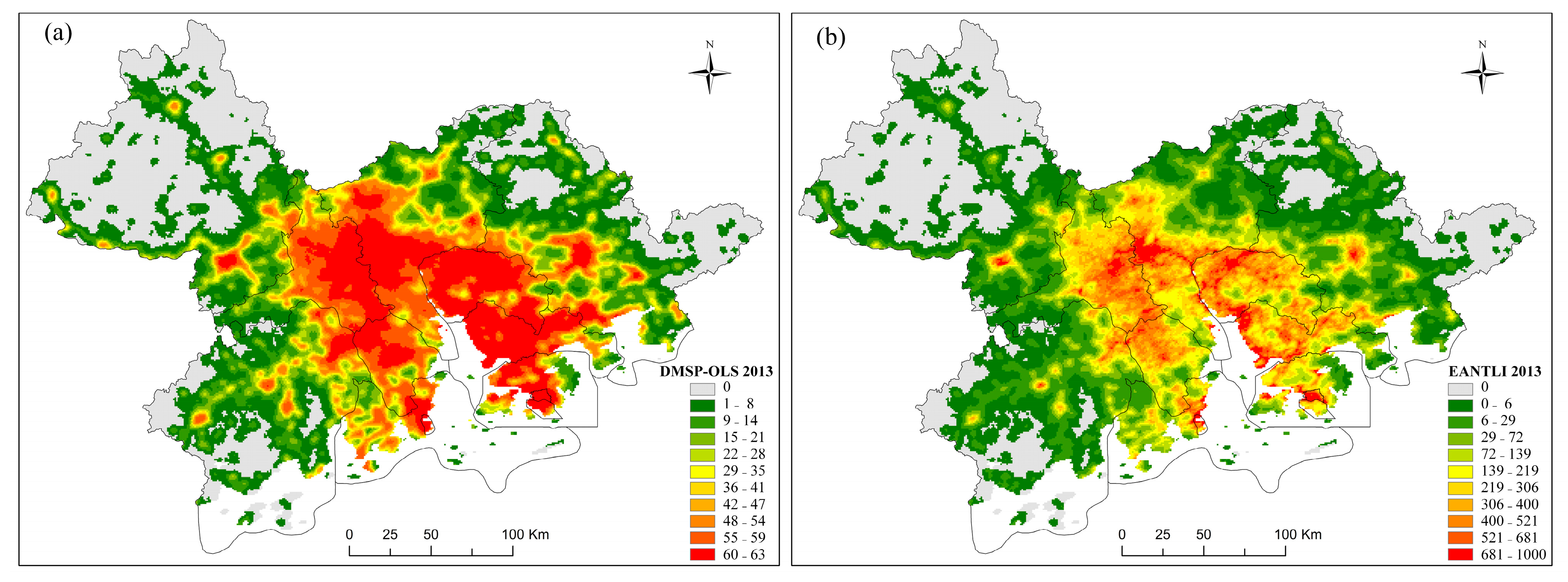
The saturation effect exists in NTL imagery for cities at different socioeconomic and development levels. Figure 3 and Figure 4 demonstrate the saturation correction effects, intra-annual correction, and inter-annual correction on DMSP-OLS data for the Guangdong–Hong Kong–Macao Greater Bay region. As displayed in Figure 3a, DMSP-OLS images show little variation in the DN value in certain areas, especially around the cities of Guangzhou, Dongguan, Shenzhen, Hong Kong, Foshan, and Zhongshan. Meanwhile, as shown in Figure 3b, the extended value range in the EANTLI image leads to improved DN value distinguishability. Figure 4 presents four major cities where the DN values from DMSP-OLS were capped at 63. The corresponding EANTLI images, however, display mitigated saturation results, evidenced by the heterogeneity.
3.2. VIIRS Time Series Decomposition with STL
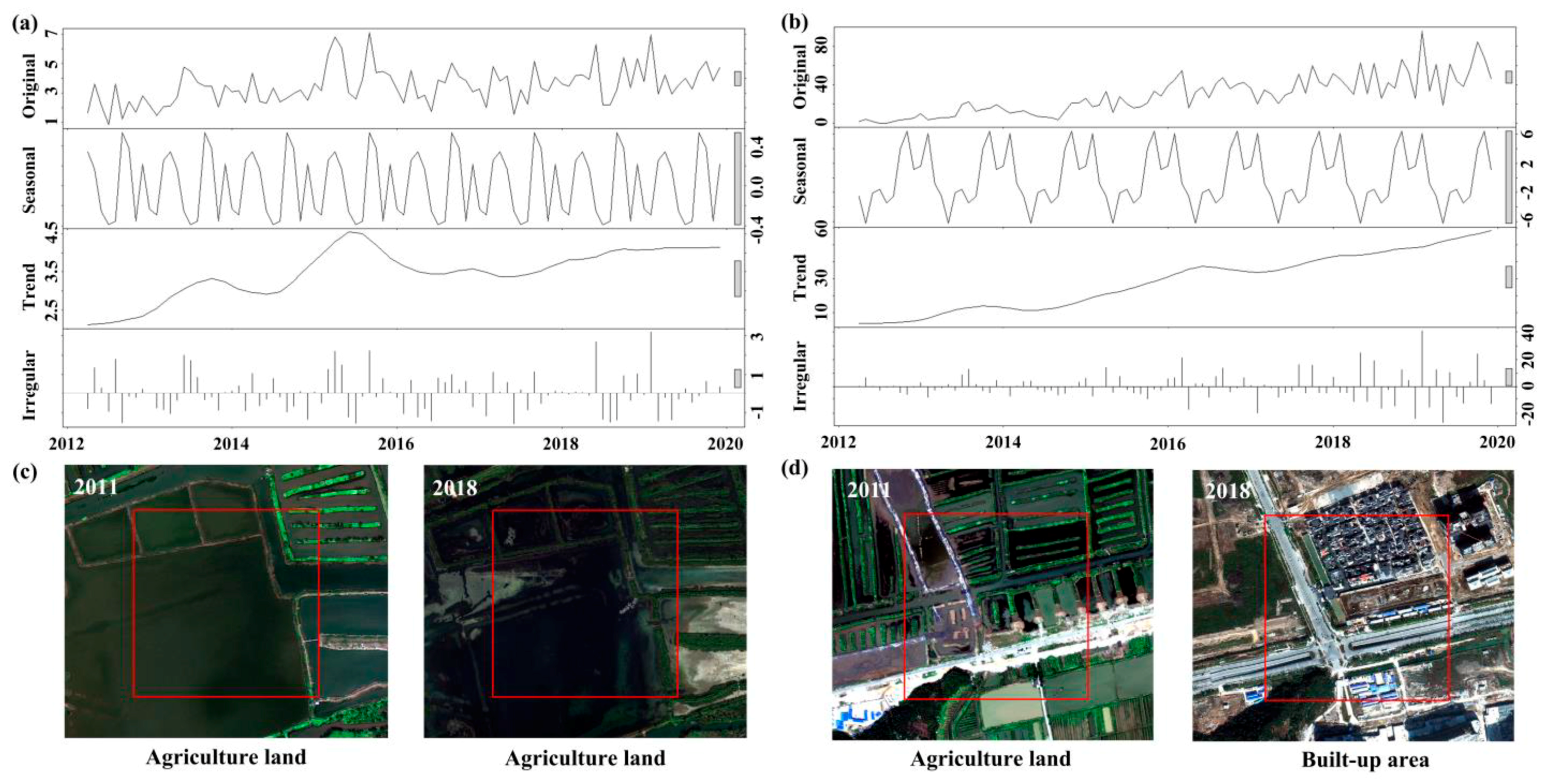
Figure 5 demonstrates the results of VIIRS time series decomposition with STL, given different changing patterns of land coverage. Seasonal, trend, and irregular components are successfully separated. Bars to the right side of each plot in Figure 5 have the same length but have relatively different sizes as they are plotted on different scales. The long bars in the seasonal plots indicate that the time series decompose the prominence seasonality signal, which illustrates the necessity to strip away the seasonal components to obtain the trend components. The seasonal and irregular signals can be clearly observed, as the sum of seasonal and irregular components accounted for 23.70% and 27.50% of the original VIIRS time series in Figure 5a,b, respectively. These irregular components (i.e., the abnormal increase in values in June 2018 and February 2019) affected monthly VIIRS time series, presumably leading to calculation errors. STL is able to detect trend components and seasonal components, thus removing the impacts from these outliers in the original time series. The above results suggest that removing seasonal and irregular components from monthly VIIRS data via STL is a necessary step to obtain consistent yearly VIIRS products.
3.3. Evaluation of the Intercalibration Model
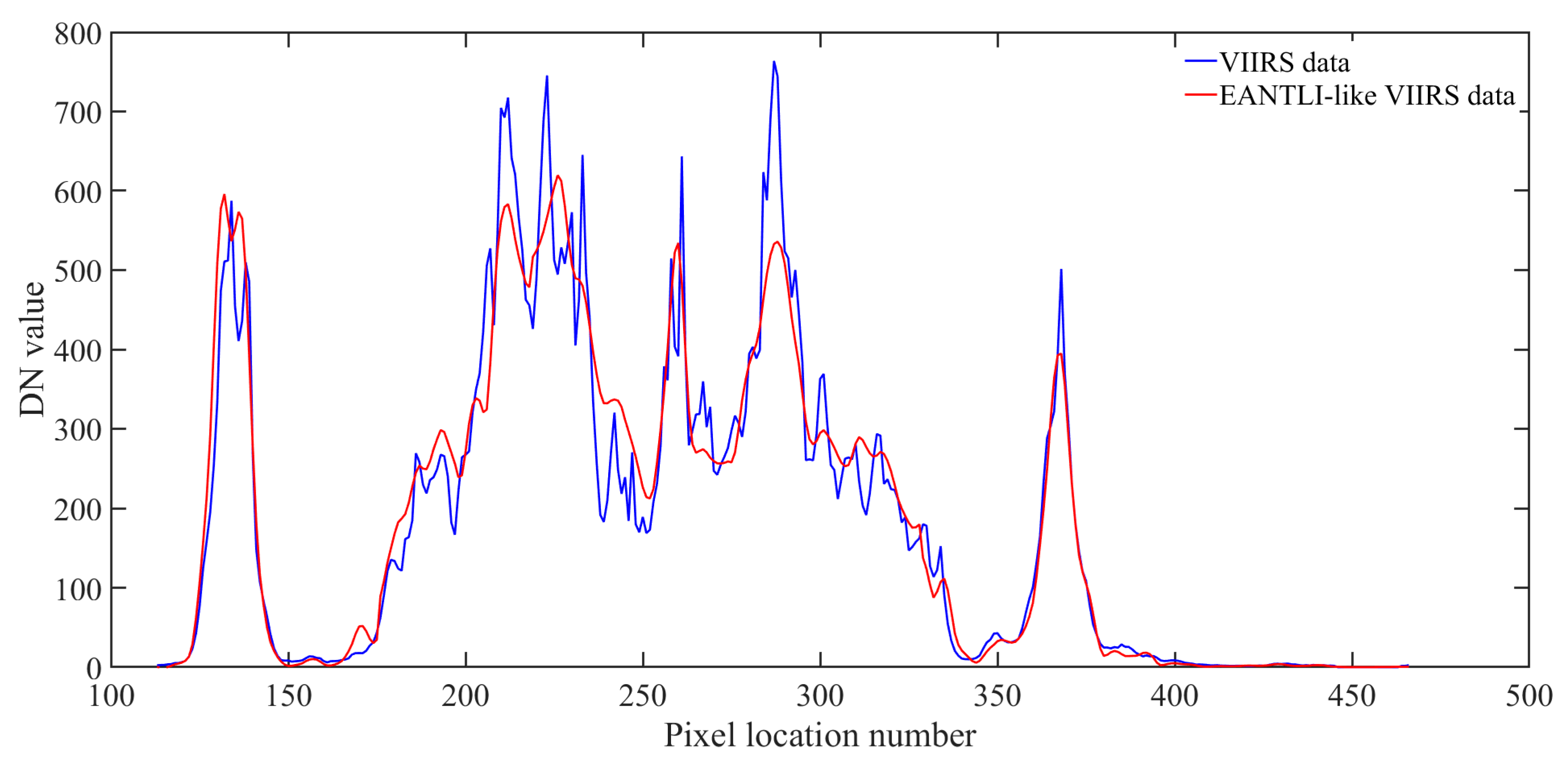
Based on the GWR model, we constructed an intercalibration model linking EANTLI and VIIRS to obtain EANTLI-like VIIRS data. The Guangdong–Hong Kong–Macao Greater Bay region has experienced rapid development and urbanization in the past decades, which led to significant differences in the socioeconomic development of the cities in this area. Thus, we constructed GWR models according to the city size and its economic development. The study area was divided into seven zones, including Foshan, Huizhou, Jiangmen, Zhaoqing, Zhongshan_Zhuhai_Macao, Shenzhen_Hong Kong, and Guangzhou_Dongguan. Table 1 shows the performance of GWR models for seven zones, as well as for the entire study area. Indicators to evaluate the performance consist of MAE, RMSE, Pearson’s coefficient, and R2. Using the intercalibration models, we derived the EANTLI-like VIIRS data in 2014–2019. Figure 6 shows the DN value distribution between the EANTLI-like VIIRS data and the EANTLI data along the latitudinal transect. The results demonstrate that EANTLI-like VIIRS data present similar DN values and are capable of expressing considerable heterogeneity, suggesting that the intercalibration models we constructed are effective.
3.4. ISA% Mapping
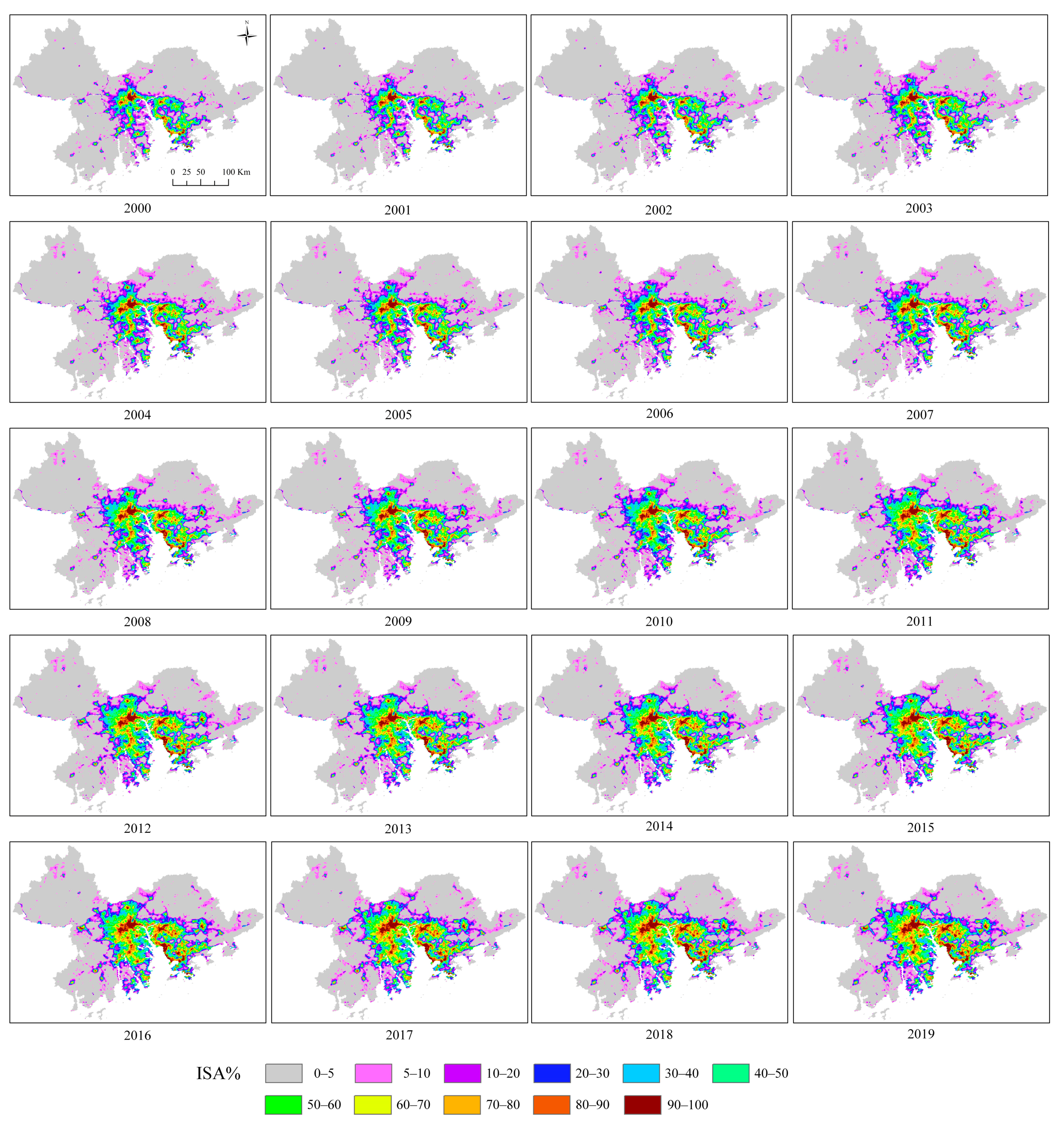
In this study, the GA-BP model was applied to map annual ISA% from 2000 to 2019. For BP neural network, NTL, LST, NDBVI, and population data served as input feature datasets. The reference dataset of impervious surface coverage derived from Landsat images was used as the output. A three-layer neural network was applied with four input layers, six hidden layers, and one output layer. In the genetic algorithm, the population size, crossover rate, and mutation rate were set as 50, 0.2, and 0.1, respectively. The yearly ISA% distribution over the study period was divided into eleven grades, as shown in Figure 7. Figure 7 shows that the ISA% increased from 7.97% in 2000 to 17.11% in 2019 in the Greater Bay region, consistent with the pattern of explosive growth. The investigated temporal period was divided into four stages: (1) 2000–2002; (2) 2003–2009; (3) 2010–2015; (4) 2016–2019. The average annual growth rate of ISA% at each stage varied from 8.45%, 3.88%, 3.13%, to 2.28%, indicating a downward trajectory in the urbanization process.
Cities with a lower level of economic development, such as Huizhou, Zhaoqing, Jiangmen, Zhuhai, and Zhongshan, experienced increased ISA% especially in urban cores, and the average annual growth rate of ISA% in these cities have increased dramatically. In Guangzhou, Shenzhen, Foshan, and Dongguan, zones with a particularly high speed of urbanization, impervious surfaces expanded from urban cores to suburban areas, so the average annual growth rate of ISA% maintained relatively stable. In comparison, Hong Kong and Macau are in a mature period of impervious surface expansion, as they already reached a high level of urbanization before 2000. Impervious surfaces in Hong Kong and Macau demonstrated a slight expansion during the investigated period, with a relatively slow average annual growth rate of ISA% and unchanged ISA spatial patterns.
4. Discussion
4.1. Accuracy Assessment
We compared our estimated ISA% maps with the GAIA 1985–2018 and FROM-GLC10 products developed by Gong et al. [28,70]. In their researches, Gong et al. [28] utilized Landsat images and ancillary datasets that consist of NTL data and the Sentinel-1 Synthetic Aperture Radar data to develop an automatic mapping procedure on the Google Earth Engine (GEE) platform to provide annual global artificial impervious areas (GAIA) from 1985 to 2018 at a 30 m resolution. Additionally, Gong et al. [70] developed FROM-GLC10 by transferring a training sample set of 2015 at 30 m resolution to classify 10 m resolution images of 2017.
To quantitatively assess the performance of our model in estimating ISA% maps, 500 samples from historical Landsat images were interpreted to calculate MAE, RMSE, Pearson’s coefficient, and R2 between the ground-truth values and predicted values derived from different products. Table 2 displays the accuracy assessment results.
As shown in Table 2, our model achieved effective performance with a MAE of 0.0647 (slight overestimation), RMSE of 0.1003, Pearson’s coefficient of 0.9613, and R2 of 0.9239, outperforming FROM-GLC10 and GAIA 1985–2018 (except for the MAE of GAIA 1985–2018).
4.2. Spatiotemporal Analysis of ISA% during 2000–2019
As Figure 8 shows, all Global Moran’s I values are positive, indicating significant spatial autocorrelation of ISA% across the entire Greater Bay region, as well as in each city during 2000–2019 (Given the small size of Macau, its Global Moran’s I and local Moran’s I were not calculated). In the entire Greater Bay region, the Global Moran’s I increased from 0.734 in 2000 to 0.7997 in 2010, suggesting notably increased spatial autocorrelation in ISA%, with a relatively stable trend from 2011 to 2019. When it comes to the city scale, Global Moran’s I value showed variation over time.
As shown in Figure 8, the degree of spatial autocorrelation of ISA% in Guangzhou and Foshan was significantly higher than in the other cities. As the capital of Guangdong Province, Guangzhou demonstrated a relatively stable trend, while the degree of spatial autocorrelation of ISA% in Foshan increased from 0.7717 in 2000 to 0.8693 in 2019. Huizhou and Zhaoqing witnessed a higher growth rate compared to cities. The Global Moran’s I of Huizhou increased from 0.4441 to 0.6561, whereas the Global Moran’s I of Zhaoqing increased from 0.3769 to 0.5574 over these 20 years. Jiangmen also showed an upward trend in the Global Moran’s I value, while the value in Zhongshan changed from 0.4928 to 0.5959. The degree of spatial autocorrelation in Hong Kong demonstrated a relatively steady trend. The degree of spatial autocorrelation in Dongguan jumped in the first eight years of the study period and then showed a slight downward tendency. Similar patterns can be seen in Shenzhen. Compared to all other cities, Zhuhai stands out, given its continuously declining degree of spatial autocorrelation of ISA% during the study period.
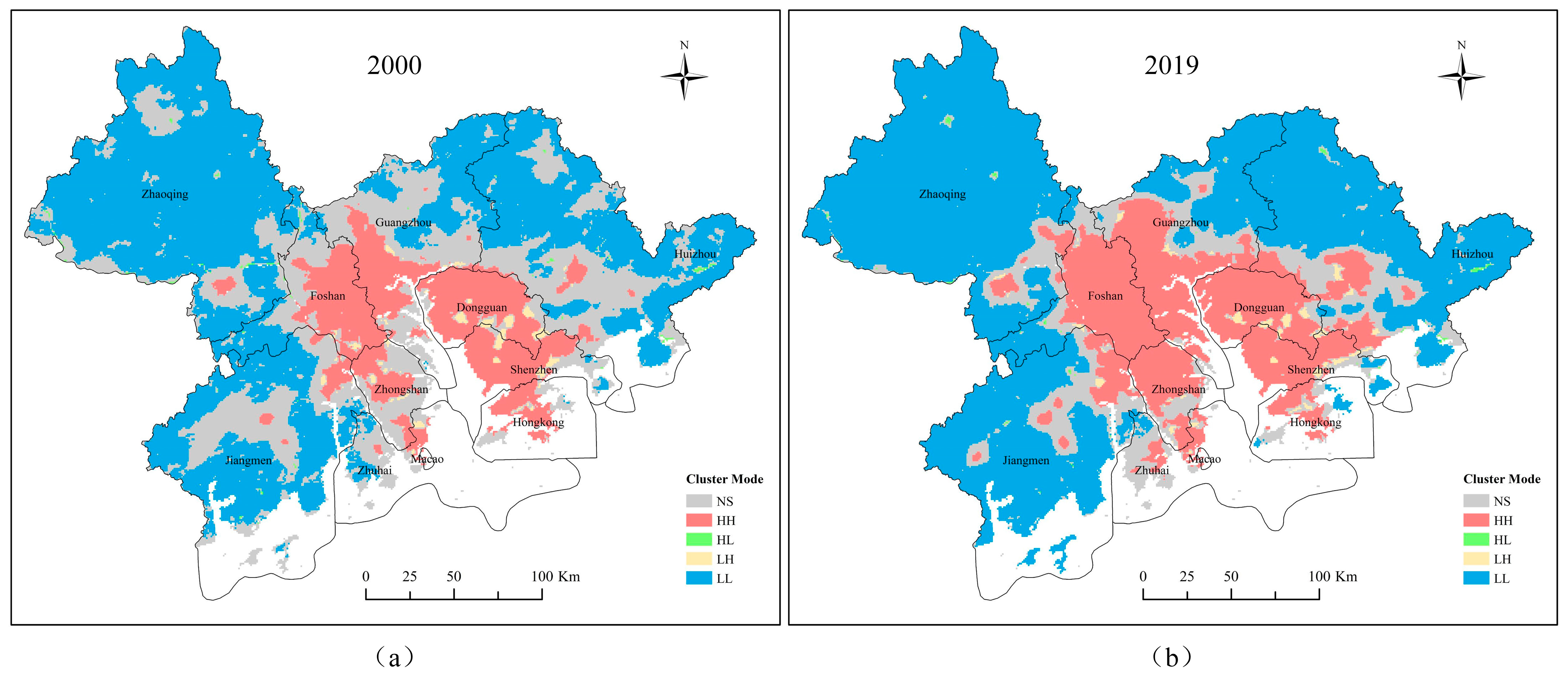
Figure 9 shows Local Moran’s I indices of the Greater Bay in 2000 and 2019, with detected spatial cluster modes. NS indicates insignificant cluster mode. HH represents the spatial clustering of high ISA% values. HL suggests that a grid with a high ISA% is surrounded by ones with a low ISA%. LH suggests that a grid with low ISA% is surrounded by ones with high ISA%. LL indicates the spatial clustering of low ISA% values. We can observe the HH clusters are distributed in Guangzhou, Foshan, Zhongshan, Dongguan, Shenzhen, and Hong Kong, while the LL clusters exist in Zhaoqing, Jiangmen, Huizhou, and the north of Guangzhou.
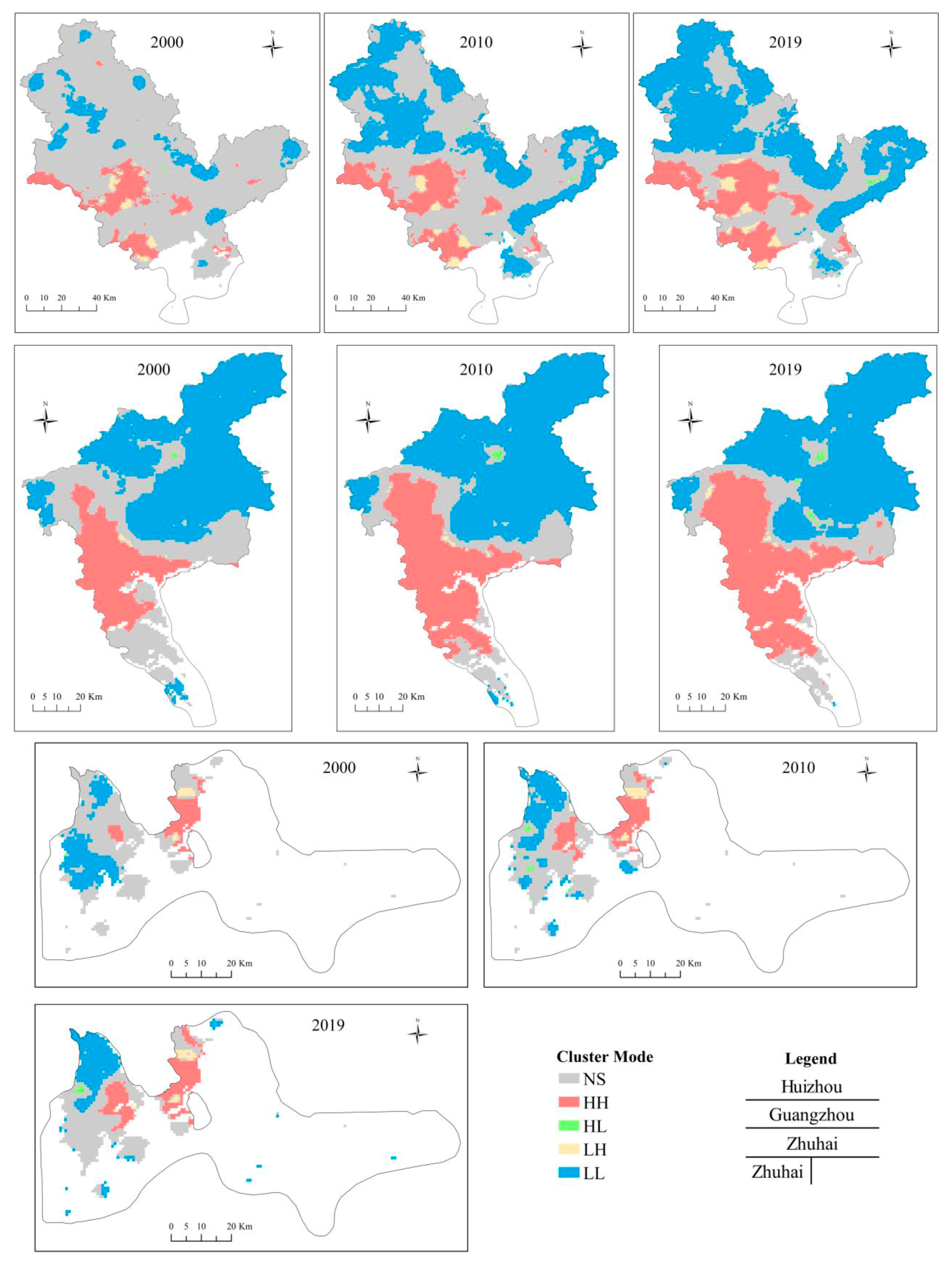
Distinctive changes in the HH cluster appear in ISA% for Guangzhou, Foshan, Jiangmen, Zhongshan, and Huizhou, suggest a considerably increased ISA%. In addition, we calculated the Local Moran’s I for Huizhou, Guangzhou, and Zhuhai. We selected these three cities because of their representativeness, given their different urbanization and levels of spatial autocorrelation in the ISA%. The changes in their spatial clustering of ISA% over time are displayed in Figure 10. We observed a notable change in HH clusters from 2000 to 2019 in Huizhou. The expansion of HH clusters in Guangzhou demonstrated an uptrend from 2000 to 2010 but maintained a stable level from 2010 to 2019. In comparison, changes in Zhuhai were not as clear as in the other two cities.
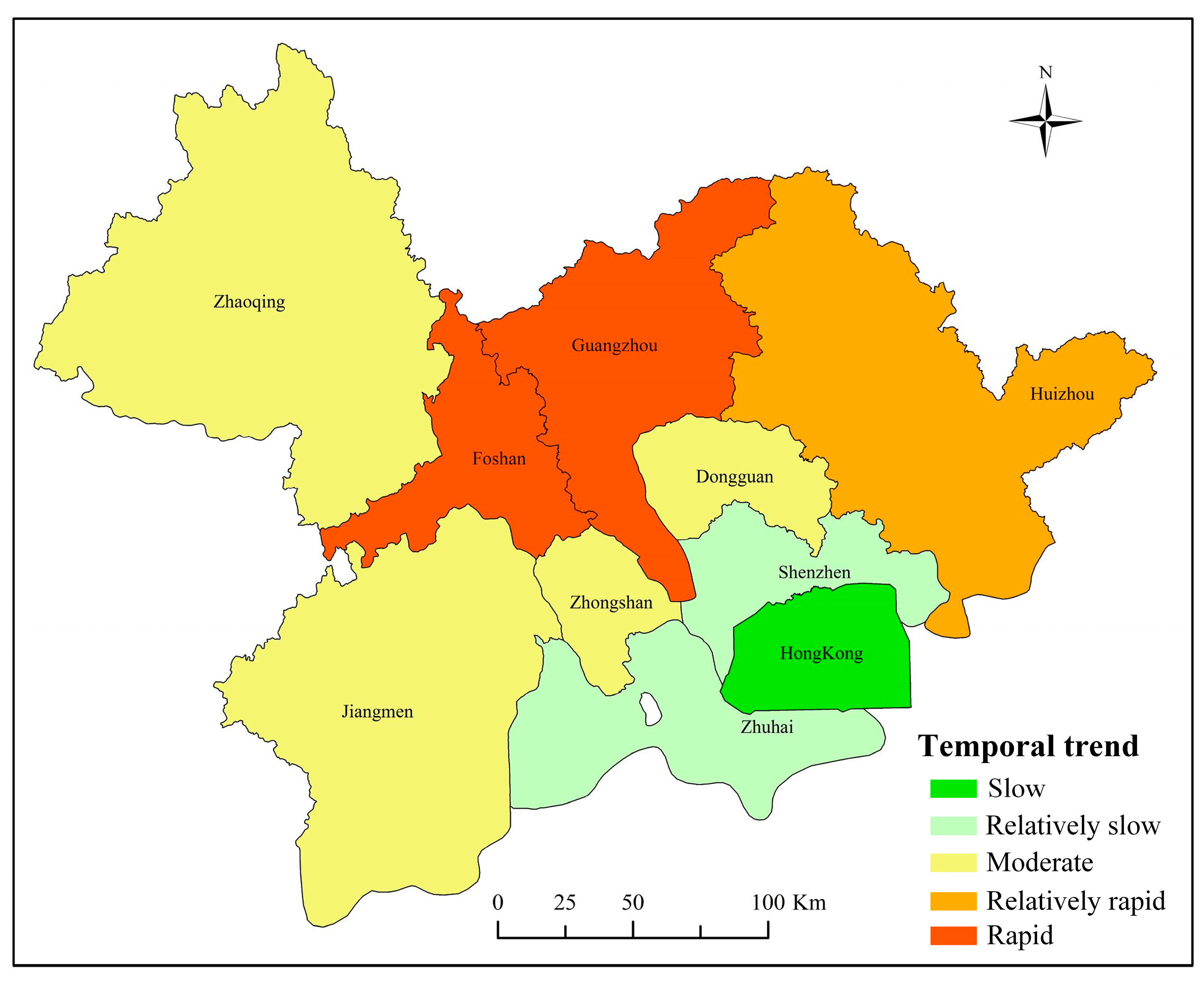
Figure 11 shows the temporal variation of the ISA% in different cities from 2000 to 2019. Rapid growth occurred in Guangzhou and Foshan, corresponding to their high rate of urbanization during these 20 years. As the three cities with the lowest per capita gross domestic product in the Greater Bay in 2018, Zhaoqing and Jiangmen experienced moderate growth, and Huizhou demonstrated relatively stable growth in ISA%.
5. Conclusions
The complexity of impervious surface features impedes mapping at the regional and global scale. NTL images, as an emerging data source, have been shown to be a reliable data source for mapping ISA. Nevertheless, we need to properly deal with saturation and blooming problems, as well as the inconsistency in DMSP-OLS data. In addition, calibrations are needed before a long-term, consistent NTL time series can be formed to ensure the compatibility and comparability of images from DMSP-OLS and VIIRS satellite sensors. Furthermore, ISA extraction based on single-source remote sensing data has widely recognized limitations that include low adaptability and low universality. Therefore, we made the following improvements. (1) We used EANTLI to address the saturation and blooming issues in DMSP-OLS data. Intra-annual and inter-annual corrections were performed to address the inconsistencies in lighted pixels. (2) We generated long-term and consistent NTL data from 2000 to 2019 by combining EANTLI and VIIRS. The trend components of monthly VIIRS data were extracted and used to build a cross-sensor calibration model based on the GWR model. (3) We utilized multisource temporal features extracted from consistent NTL data, MODIS, and population data to establish an ISA% estimation model.
Taking the Guangdong–Hong Kong–Macao Greater Bay region as a study area, the proposed method was utilized to map ISA% from 2000 to 2019. The results indicate that ISA% in the study area increased from 7.97% in 2000 to 17.11% in 2019. An accuracy assessment shows that our proposed method achieves great performance in ISA% mapping, with MAE of 0.0647, RMSE of 0.1003, Pearson’s coefficient of 0.9613, and of 0.9239. A spatiotemporal analysis of ISA% reveals significant spatial autocorrelation in the entire Greater Bay, as well as in each city during the investigated 20-year period. Thus, we infer that cities experienced divergent patterns in ISA% change over time.
Our method can be used to generate high-frequency ISA% maps at a large scale due to its ease of implementation and the availability of data sources. These high-frequency ISA% maps can be used to analyze the socioeconomic, environmental dynamics, and urban processes at a regional or global scale. As more NTL satellite sensors are starting to emerge at improved spatiotemporal resolutions, we need to improve inter-calibrating methods to reduce the incompatibility of different NTL data sources.
Author Contributions
Conceptualization, Y.T. and Z.S.; methodology, Y.T.; software, Y.T. and B.C.; formal analysis, Y.T.; investigation, Y.T.; resources, Z.S.; data curation, Y.T. and B.C.; writing—original draft preparation, Y.T.; writing—review and editing, Y.T., X.H.; visualization, Y.T.; supervision, Z.S.; project administration, Z.S.; funding acquisition, Z.S. All authors have read and agreed to the published version of the manuscript.
Funding
This research was funded by the National Key Research and Development Program of China with grant number 2018YFB2100501, the Key Research and Development Program of Yunnan province in China with grant number 2018IB023, the National Natural Science Foundation of China with grant numbers 42090012, 41771452, 41771454 and 41890820.
Acknowledgments
The authors are sincerely grateful to the editors, as well as the anonymous reviewers, for their valuable suggestions and comments that helped us improve this paper significantly.
Conflicts of Interest
The authors declare no conflict of interest.
References
- Nations, U. World Urbanization Prospects: The 2014 Revision, Highlights; Department of Economic and Social Affairs, Population Division, United Nations: New York, NY, USA, 2014; Volume 32. [Google Scholar]
- Kuang, W.L.J.; Zhang, Z.; Lu, D.; Xiang, B. Spatiotemporal dynamics of impervious surface areas across China during the early 21st century. Chin. Sci. Bull. 2012, 58, 1691–1701. [Google Scholar] [CrossRef] [Green Version]
- Cao, X.W.J.; Chen, J.; Shi, F. Spatialization of electricity consumption of China using saturation-corrected DMSP-OLS data. Int. J. Appl. Earth Obs. Geoinf. 2014, 28, 193–200. [Google Scholar] [CrossRef]
- National Bureau of Statistics of China. China Statistical Yearbook 2020; China Statistics Press: Beijing, China, 2020.
- Deng, C.; Wu, C. Examining the impacts of urban biophysical compositions on surface urban heat island: A spectral unmixing and thermal mixing approach. Remote Sens. Environ. 2013, 131, 262–274. [Google Scholar] [CrossRef]
- Kaufmann, R.K.; Seto, K.C.; Schneider, A.; Liu, Z.; Zhou, L.; Wang, W. Climate response to rapid urban growth: Evidence of a human-induced precipitation deficit. J. Clim. 2007, 20, 2299–2306. [Google Scholar] [CrossRef]
- Yuan, F.; Bauer, M.E. Comparison of impervious surface area and normalized difference vegetation index as indicators of surface urban heat island effects in Landsat imagery. Remote Sens. Environ. 2007, 106, 375–386. [Google Scholar] [CrossRef]
- Li, X.; Zhou, Y.; Asrar, G.R.; Mao, J.; Li, X.; Li, W. Response of vegetation phenology to urbanization in the conterminous United States. Glob. Chang. Biol. 2017, 23, 2818–2830. [Google Scholar] [CrossRef] [PubMed]
- Liu, C.; Luo, H.; Yao, Y. Optimizing subpixel impervious surface area mapping through adaptive integration of spectral, phenological, and spatial features. IEEE Geosci. Remote Sens. Lett. 2017, 14, 1017–1021. [Google Scholar] [CrossRef]
- Shi, K.; Yu, B.; Huang, Y.; Hu, Y.; Yin, B.; Chen, Z.; Chen, L.; Wu, J. Evaluating the ability of NPP-VIIRS nighttime light data to estimate the gross domestic product and the electric power consumption of China at multiple scales: A comparison with DMSP-OLS data. Remote Sens. 2014, 6, 1705–1724. [Google Scholar] [CrossRef] [Green Version]
- Chithra, S.; Nair, M.H.; Amarnath, A.; Anjana, N. Impacts of impervious surfaces on the environment. Int. J. Eng. Sci. Invent. 2015, 4, 2319–6726. [Google Scholar]
- Haustein, M.D. The Urban-Rural Environment: Effects of Impervious Surface Land Cover on Lake Ecosystems. 2010. Available online: https://hdl.handle.net/11299/103264 (accessed on 7 December 2020).
- Shao, Z.; Fu, H.; Li, D.; Altan, O.; Cheng, T. Remote sensing monitoring of multi-scale watersheds impermeability for urban hydrological evaluation. Remote Sens. Environ. 2019, 232, 111338. [Google Scholar] [CrossRef]
- Srinivasan, V.; Seto, K.C.; Emerson, R.; Gorelick, S.M. The impact of urbanization on water vulnerability: A coupled human–environment system approach for Chennai, India. Glob. Environ. Chang. 2013, 23, 229–239. [Google Scholar] [CrossRef]
- Lu, D.; Li, G.; Moran, E.; Batistella, M.; Freitas, C.C. Mapping impervious surfaces with the integrated use of Landsat Thematic Mapper and radar data: A case study in an urban–rural landscape in the Brazilian Amazon. ISPRS J. Photogramm. Remote Sens. 2011, 66, 798–808. [Google Scholar] [CrossRef] [Green Version]
- Shao, Z.; Liu, C. The integrated use of DMSP-OLS nighttime light and MODIS data for monitoring large-scale impervious surface dynamics: A case study in the Yangtze River Delta. Remote Sens. 2014, 6, 9359–9378. [Google Scholar] [CrossRef] [Green Version]
- Shao, Z.; Fu, H.; Fu, P.; Yin, L. Mapping urban impervious surface by fusing optical and SAR data at the decision level. Remote Sens. 2016, 8, 945. [Google Scholar] [CrossRef] [Green Version]
- Wu, C.; Murray, A.T. Estimating impervious surface distribution by spectral mixture analysis. Remote Sens. Environ. 2003, 84, 493–505. [Google Scholar] [CrossRef]
- Weng, Q.; Hu, X.; Lu, D. Extracting impervious surfaces from medium spatial resolution multispectral and hyperspectral imagery: A comparison. Int. J. Remote Sens. 2008, 29, 3209–3232. [Google Scholar] [CrossRef]
- Weng, Q.; Hu, X. Medium spatial resolution satellite imagery for estimating and mapping urban impervious surfaces using LSMA and ANN. IEEE Trans. Geosci. Remote Sens. 2008, 46, 2397–2406. [Google Scholar] [CrossRef]
- Slonecker, E.T.; Jennings, D.B.; Garofalo, D. Remote sensing of impervious surfaces: A review. Remote Sens. Rev. 2001, 20, 227–255. [Google Scholar] [CrossRef]
- Weng, Q. Remote sensing of impervious surfaces in the urban areas: Requirements, methods, and trends. Remote Sens. Environ. 2012, 117, 34–49. [Google Scholar] [CrossRef]
- Wang, Y.; Li, M. Urban impervious surface detection from remote sensing images: A review of the methods and challenges. IEEE Geosci. Remote Sens. Mag. 2019, 7, 64–93. [Google Scholar] [CrossRef]
- Powell, S.L.; Cohen, W.B.; Yang, Z.; Pierce, J.D.; Alberti, M. Quantification of impervious surface in the Snohomish water resources inventory area of western Washington from 1972–2006. Remote Sens. Environ. 2008, 112, 1895–1908. [Google Scholar] [CrossRef] [Green Version]
- Sexton, J.O.; Song, X.-P.; Huang, C.; Channan, S.; Baker, M.E.; Townshend, J.R. Urban growth of the Washington, DC–Baltimore, MD metropolitan region from 1984 to 2010 by annual, Landsat-based estimates of impervious cover. Remote Sens. Environ. 2013, 129, 42–53. [Google Scholar] [CrossRef]
- Zhang, L.; Weng, Q. Annual dynamics of impervious surface in the Pearl River Delta, China, from 1988 to 2013, using time series Landsat imagery. ISPRS J. Photogramm. Remote Sens. 2016, 113, 86–96. [Google Scholar] [CrossRef]
- Zhang, L.; Weng, Q.; Shao, Z. An evaluation of monthly impervious surface dynamics by fusing Landsat and MODIS time series in the Pearl River Delta, China, from 2000 to 2015. Remote Sens. Environ. 2017, 201, 99–114. [Google Scholar] [CrossRef]
- Gong, P.; Li, X.; Wang, J.; Bai, Y.; Chen, B.; Hu, T.; Liu, X.; Xu, B.; Yang, J.; Zhang, W. Annual maps of global artificial impervious area (GAIA) between 1985 and 2018. Remote Sens. Environ. 2020, 236, 111510. [Google Scholar] [CrossRef]
- Lawrence, W. A technique for using composite DMSP/OLS’city lights’ satellite data to accurately map urban areas. Remote Sens. Environ. 1997, 61, 361–370. [Google Scholar]
- Zhu, Z.; Zhou, Y.; Seto, K.C.; Stokes, E.C.; Deng, C.; Pickett, S.T.; Taubenböck, H. Understanding an urbanizing planet: Strategic directions for remote sensing. Remote Sens. Environ. 2019, 228, 164–182. [Google Scholar] [CrossRef]
- Small, C.; Elvidge, C.D. Night on Earth: Mapping decadal changes of anthropogenic night light in Asia. Int. J. Appl. Earth Obs. Geoinf. 2013, 22, 40–52. [Google Scholar] [CrossRef] [Green Version]
- Bennie, J.; Davies, T.W.; Duffy, J.P.; Inger, R.; Gaston, K.J. Contrasting trends in light pollution across Europe based on satellite observed night time lights. Sci. Rep. 2014, 4, 1–6. [Google Scholar] [CrossRef] [Green Version]
- Li, X.; Liu, S.; Jendryke, M.; Li, D.; Wu, C. Night-time light dynamics during the iraqi civil war. Remote Sens. 2018, 10, 858. [Google Scholar] [CrossRef] [Green Version]
- Hu, T.; Huang, X. A novel locally adaptive method for modeling the spatiotemporal dynamics of global electric power consumption based on DMSP-OLS nighttime stable light data. Appl. Energy 2019, 240, 778–792. [Google Scholar] [CrossRef]
- Agnew, J.; Gillespie, T.W.; Gonzalez, J.; Min, B. Baghdad nights: Evaluating the U.S. military ‘surge’using nighttime light signatures. Environ. Plan. A 2008, 40, 2285–2295. [Google Scholar] [CrossRef]
- Li, X.; Li, D. Can night-time light images play a role in evaluating the Syrian Crisis? Int. J. Remote Sens. 2014, 35, 6648–6661. [Google Scholar] [CrossRef]
- Elvidge, C.D.; Tuttle, B.T.; Sutton, P.C.; Baugh, K.E.; Howard, A.T.; Milesi, C.; Bhaduri, B.; Nemani, R. Global distribution and density of constructed impervious surfaces. Sensors 2007, 7, 1962–1979. [Google Scholar] [CrossRef]
- Chen, Z.; Yu, B.; Zhou, Y.; Liu, H.; Yang, C.; Shi, K.; Wu, J. Mapping global urban areas from 2000 to 2012 using time-series nighttime light data and MODIS products. IEEE J. Sel. Top. Appl. Earth Obs. Remote Sens. 2019, 12, 1143–1153. [Google Scholar] [CrossRef]
- Lu, D.; Tian, H.; Zhou, G.; Ge, H. Regional mapping of human settlements in southeastern China with multisensor remotely sensed data. Remote Sens. Environ. 2008, 112, 3668–3679. [Google Scholar] [CrossRef]
- Guo, W.; Lu, D.; Wu, Y.; Zhang, J. Mapping impervious surface distribution with integration of SNNP VIIRS-DNB and MODIS NDVI data. Remote Sens. 2015, 7, 12459–12477. [Google Scholar] [CrossRef] [Green Version]
- Henderson, M.; Yeh, E.T.; Gong, P.; Elvidge, C.; Baugh, K. Validation of urban boundaries derived from global night-time satellite imagery. Int. J. Remote Sens. 2003, 24, 595–609. [Google Scholar] [CrossRef]
- Small, C.; Pozzi, F.; Elvidge, C.D. Spatial analysis of global urban extent from DMSP-OLS night lights. Remote Sens. Environ. 2005, 96, 277–291. [Google Scholar] [CrossRef]
- Zhou, Y.; Smith, S.J.; Zhao, K.; Imhoff, M.; Thomson, A.; Bond-Lamberty, B.; Asrar, G.R.; Zhang, X.; He, C.; Elvidge, C.D. A global map of urban extent from nightlights. Environ. Res. Lett. 2015, 10, 054011. [Google Scholar] [CrossRef]
- Cao, X.; Chen, J.; Imura, H.; Higashi, O. A SVM-based method to extract urban areas from DMSP-OLS and SPOT VGT data. Remote Sens. Environ. 2009, 113, 2205–2209. [Google Scholar] [CrossRef]
- Zhou, Y.; Smith, S.J.; Elvidge, C.D.; Zhao, K.; Thomson, A.; Imhoff, M. A cluster-based method to map urban area from DMSP/OLS nightlights. Remote Sens. Environ. 2014, 147, 173–185. [Google Scholar] [CrossRef]
- Li, Q.; Lu, L.; Weng, Q.; Xie, Y.; Guo, H. Monitoring urban dynamics in the southeast USA using time-series DMSP/OLS nightlight imagery. Remote Sens. 2016, 8, 578. [Google Scholar] [CrossRef] [Green Version]
- Xie, Y.; Weng, Q. Updating urban extents with nighttime light imagery by using an object-based thresholding method. Remote Sens. Environ. 2016, 187, 1–13. [Google Scholar] [CrossRef]
- Zhuo, L.; Zheng, J.; Zhang, X.; Li, J.; Liu, L. An improved method of night-time light saturation reduction based on EVI. Int. J. Remote Sens. 2015, 36, 4114–4130. [Google Scholar] [CrossRef]
- Zhang, Q.; Schaaf, C.; Seto, K.C. The vegetation adjusted NTL urban index: A new approach to reduce saturation and increase variation in nighttime luminosity. Remote Sens. Environ. 2013, 129, 32–41. [Google Scholar] [CrossRef]
- Guo, W.; Lu, D.; Kuang, W. Improving fractional impervious surface mapping performance through combination of DMSP-OLS and MODIS NDVI data. Remote Sens. 2017, 9, 375. [Google Scholar] [CrossRef] [Green Version]
- Cao, W.; Dong, L.; Wu, L.; Liu, Y. Quantifying urban areas with multisource data based on percolation theory. Remote Sens. Environ. 2020, 241, 111730. [Google Scholar] [CrossRef] [Green Version]
- Li, X.; Li, D.; Xu, H.; Wu, C. Intercalibration between DMSP/OLS and VIIRS night-time light images to evaluate city light dynamics of Syria’s major human settlement during Syrian Civil War. Int. J. Remote Sens. 2017, 38, 5934–5951. [Google Scholar] [CrossRef]
- Zheng, Q.; Weng, Q.; Wang, K. Developing a new cross-sensor calibration model for DMSP-OLS and Suomi-NPP VIIRS night-light imageries. ISPRS J. Photogramm. Remote Sens. 2019, 153, 36–47. [Google Scholar] [CrossRef]
- Yang, G.; Zhao, Y.; Xing, H.; Fu, Y.; Liu, G.; Kang, X.; Mai, X. Understanding the changes in spatial fairness of urban greenery using time-series remote sensing images: A case study of Guangdong-Hong Kong-Macao Greater Bay. Sci. Total Environ. 2020, 715, 136763. [Google Scholar] [CrossRef]
- Huang, X.; Wang, C.; Lu, J. Understanding the spatiotemporal development of human settlement in hurricane-prone areas on the US Atlantic and Gulf coasts using nighttime remote sensing. Nat. Hazards Earth Syst. Sci. 2019, 19, 2141–2155. [Google Scholar] [CrossRef] [Green Version]
- Elvidge, C.D.; Baugh, K.E.; Dietz, J.B.; Bland, T.; Sutton, P.C.; Kroehl, H.W. Radiance calibration of DMSP-OLS low-light imaging data of human settlements. Remote Sens. Environ. 1999, 68, 77–88. [Google Scholar] [CrossRef]
- Elvidge, C.D.; Baugh, K.E.; Zhizhin, M.; Hsu, F.-C. Why VIIRS data are superior to DMSP for mapping nighttime lights. Proc. Asia-Pac. Adv. Netw. 2013, 35, 62. [Google Scholar] [CrossRef] [Green Version]
- He, C.; Shi, P.; Xie, D.; Zhao, Y. Improving the normalized difference built-up index to map urban built-up areas using a semiautomatic segmentation approach. Remote Sens. Lett. 2010, 1, 213–221. [Google Scholar] [CrossRef] [Green Version]
- Tatem, A.J. WorldPop, open data for spatial demography. Sci. Data 2017, 4, 1–4. [Google Scholar] [CrossRef]
- Leyk, S.; Gaughan, A.E.; Adamo, S.B.; Sherbinin, A.d.; Balk, D.; Freire, S.; Rose, A.; Stevens, F.R.; Blankespoor, B.; Frye, C. The spatial allocation of population: A review of large-scale gridded population data products and their fitness for use. Earth Syst. Sci. Data 2019, 11, 1385–1409. [Google Scholar] [CrossRef] [Green Version]
- Li, K.; Chen, Y.; Li, Y. The random forest-based method of fine-resolution population spatialization by using the international space station nighttime photography and social sensing data. Remote Sens. 2018, 10, 1650. [Google Scholar] [CrossRef] [Green Version]
- Pok, S.; Matsushita, B.; Fukushima, T. An easily implemented method to estimate impervious surface area on a large scale from MODIS time-series and improved DMSP-OLS nighttime light data. ISPRS J. Photogramm. Remote Sens. 2017, 133, 104–115. [Google Scholar] [CrossRef] [Green Version]
- Shi, K.; Chen, Y.; Yu, B.; Xu, T.; Yang, C.; Li, L.; Huang, C.; Chen, Z.; Liu, R.; Wu, J. Detecting spatiotemporal dynamics of global electric power consumption using DMSP-OLS nighttime stable light data. Appl. Energy 2016, 184, 450–463. [Google Scholar] [CrossRef]
- Levin, N.; Zhang, Q. A global analysis of factors controlling VIIRS nighttime light levels from densely populated areas. Remote Sens. Environ. 2017, 190, 366–382. [Google Scholar] [CrossRef] [Green Version]
- Jiang, B.; Liang, S.; Wang, J.; Xiao, Z. Modeling MODIS LAI time series using three statistical methods. Remote Sens. Environ. 2010, 114, 1432–1444. [Google Scholar] [CrossRef]
- Cristina, S.; Cordeiro, C.; Lavender, S.; Costa Goela, P.; Icely, J.; Newton, A. MERIS phytoplankton time series products from the S.W. Iberian Peninsula (Sagres) using seasonal-trend decomposition based on loess. Remote Sens. 2016, 8, 449. [Google Scholar] [CrossRef] [Green Version]
- Cleveland, R.B. STL: A seasonal-trend decomposition procedure based on loess. J. Off. Stat. 1990, 6, 3–17. [Google Scholar]
- Ding, S.; Su, C.; Yu, J. An optimizing B.P. neural network algorithm based on genetic algorithm. Artif. Intell. Rev. 2011, 36, 153–162. [Google Scholar] [CrossRef]
- Wang, S.; Zhang, N.; Wu, L.; Wang, Y. Wind speed forecasting based on the hybrid ensemble empirical mode decomposition and GA-BP neural network method. Renew. Energy 2016, 94, 629–636. [Google Scholar] [CrossRef]
- Chen, B.; Xu, B.; Zhu, Z.; Yuan, C.; Suen, H.P.; Guo, J.; Xu, N.; Li, W.; Zhao, Y.; Yang, J.; et al. Stable classification with limited sample: Transferring a 30-m resolution sample set collected in 2015 to mapping 10-m resolution global land cover in 2017. Sci. Bull. 2019, 64, 370–373. [Google Scholar]
Figure 1.
The location of the study area: Guangdong–Hong Kong–Macao Greater Bay.

Figure 2.
Flowchart of the proposed ISA% mapping model.

Figure 3.
Comparison between DMSP and EANTLI: (a) DMSP data; (b) EANTLI data.

Figure 4.
Comparison between the saturated DMSP-OLS and EANTLI data for the selected cities: (a) Guangzhou; (b) Dongguan; (c) Shenzhen; (d) Hong Kong.
Figure 4.
Comparison between the saturated DMSP-OLS and EANTLI data for the selected cities: (a) Guangzhou; (b) Dongguan; (c) Shenzhen; (d) Hong Kong.

Figure 5.
STL time series decomposition with stable land coverage (a), changed land coverage (b), WorldView images (c), and (d) for the corresponding regions. The red squares (500 m × 500 m) in (c,d) represent the corresponding location of (a,b), respectively.
Figure 5.
STL time series decomposition with stable land coverage (a), changed land coverage (b), WorldView images (c), and (d) for the corresponding regions. The red squares (500 m × 500 m) in (c,d) represent the corresponding location of (a,b), respectively.

Figure 6.
DN values of VIIRS data and EANTLI-like VIIRS data along the latitudinal transect.

Figure 7.
Dynamics of ISA% in Guangdong–Hong Kong–Macao Greater Bay, China, from 2000 to 2019.

Figure 8.
Annual dynamics of Global Moran’s I values.

Figure 9.
Changes of Local Moran’s I: (a) 2000 and (b) 2019 in the study area.

Figure 10.
Annual changes of global Moran’s I: (a) 2000 and (b) 2019 in the study area.

Figure 11.
Variation types of ISA% from 2000 to 2019 in the study area.


Table 1.
The performance of GWR models for the seven zones, as well as for the entire study area.
| Foshan | Huizhou | Jiangmen | Zhaoqing | Zhongshan_Zhuhai_Macao | Shenzhen_HongKong | Guangzhou_Dongguan | Study Area | |
|---|---|---|---|---|---|---|---|---|
| MAE | 38.2035 | 6.0587 | 5.1757 | 2.6255 | 34.4710 | 43.5085 | 28.6723 | 14.9521 |
| RMSE | 55.7511 | 17.3522 | 15.7849 | 11.9628 | 58.1819 | 79.0014 | 48.8957 | 36.5059 |
| Pearson’s coefficient | 0.9553 | 0.9656 | 0.9482 | 0.9467 | 0.9120 | 0.9139 | 0.9502 | 0.9550 |
| R2 | 0.8723 | 0.9217 | 0.8885 | 0.8765 | 0.8195 | 0.7993 | 0.9018 | 0.9115 |
Table 2.
Accuracy assessment of different models.
| MAE | RMSE | Pearson’s Coefficient | R2 | |
|---|---|---|---|---|
| Ours | 0.0647 | 0.1003 | 0.9613 | 0.9239 |
| FROM-GLC10 | 0.0982 | 0.1290 | 0.9122 | 0.8288 |
| GAIA 1985–2018 | 0.0625 | 0.1224 | 0.9494 | 0.8918 |
Publisher’s Note: MDPI stays neutral with regard to jurisdictional claims in published maps and institutional affiliations. |
© 2021 by the authors. Licensee MDPI, Basel, Switzerland. This article is an open access article distributed under the terms and conditions of the Creative Commons Attribution (CC BY) license (https://creativecommons.org/licenses/by/4.0/).
Share and Cite
MDPI and ACS Style
Tang, Y.; Shao, Z.; Huang, X.; Cai, B. Mapping Impervious Surface Areas Using Time-Series Nighttime Light and MODIS Imagery. Remote Sens. 2021, 13, 1900. https://0-doi-org.brum.beds.ac.uk/10.3390/rs13101900
AMA Style
Tang Y, Shao Z, Huang X, Cai B. Mapping Impervious Surface Areas Using Time-Series Nighttime Light and MODIS Imagery. Remote Sensing. 2021; 13(10):1900. https://0-doi-org.brum.beds.ac.uk/10.3390/rs13101900
Chicago/Turabian StyleTang, Yun, Zhenfeng Shao, Xiao Huang, and Bowen Cai. 2021. "Mapping Impervious Surface Areas Using Time-Series Nighttime Light and MODIS Imagery" Remote Sensing 13, no. 10: 1900. https://0-doi-org.brum.beds.ac.uk/10.3390/rs13101900
Note that from the first issue of 2016, this journal uses article numbers instead of page numbers. See further details here.