Impacts of Urban Expansion Forms on Ecosystem Services in Urban Agglomerations: A Case Study of Shanghai-Hangzhou Bay Urban Agglomeration

Abstract

Exploring impacts of urban expansion on ecosystem services has become a hot topic for regional sustainable development, while analyzing the ecological effects of urban expansion forms under different expansion intensities and city sizes is relatively rare. Therefore, taking a typical urban agglomeration, Shanghai-Hangzhou Bay Urban Agglomeration, as a case study, this study first analyzed the dynamics of urban expansion forms (leapfrogging, edge-expansion, and infilling) and four critical ecosystem services (carbon sequestration, food supply, habitat quality, and soil retention) in three periods from 1990 to 2019. The multiple linear regression model and zonal statistics analysis model were used to quantitatively identify the impacts of urban expansion forms on ecosystem services, taking into account different expansion intensities and city sizes. The results showed that the urban expansion trend in the study area experienced a morphological change from integration to diffusion and then to integration in 1990–2019; edge-expansion was the dominant expansion form. Food supply decreased continuously while other ecosystem services had fluctuating changes, and they all had spatial heterogeneity. The leapfrogging, edge-expansion, and infilling all had negative impacts on ecosystem services, and among them, the edge-expansion intensity had the highest influence degree in the early expansion, and the leapfrogging intensity occupied the dominant position in all influences with the expansion of urban scales. For different city sizes, the impact of edge-expansion in large-scale cities was greater than in small-scale cities in the early expansion, and the impact of leapfrogging in large-scale cities exceeded the edge-expansion in the subsequent expansion. These findings will help further understand the influential mechanisms between urban expansion and ecosystem services and provide a scientific basis for formulating reasonable urban planning.

1. Introduction

As the basis for improving the well-being of mankind and achieving sustainable development [1], ecosystem services (ESs) refer to natural conditions and utilities providing life supporting products and services by ecosystems and ecological processes that sustain anthropic life [2,3]. The changes in ESs are the most intuitive reflection of the impacts of anthropic activities on the ecological environment and directly or indirectly affect ecosystem functions, patterns, and processes [4,5]. Thus, ESs can be applied to assess the potentiality of regional ecosystems for human services and explore the changes in the ecological environment caused by human activities. Increased human activity intensity makes natural patches show a significantly and highly dispersed characteristic, which affects the functions and structures of ecosystems and results in the reduction of ESs [6]. Therefore, the assessment of ESs is important for the protection and improvement of ecological environment.

Urban expansion, an intuitive manifestation of urban development, is a land use change process that promotes the conversion of natural and semi-natural land into urban impervious surfaces [7,8]. With the population increase and economic development, the rapid urban expansion process has become one of the most prominent features of global development [9]. In China, many cities have experienced rapid growth and progressively formed urban agglomerations since the 1970s, e.g., the Yangtze River Delta Urban Agglomeration, the Pearl River Delta Urban Agglomeration, and the Beijing-Tianjin-Hebei Urban Agglomeration [10,11]. However, urban expansion areas, among the most active areas for human activities, are proved to bring the rapid transformations from ecosystems dominated by natural factors to urban ecosystems at an all-time speed and scale [12,13] and to trigger considerable changes in ESs [14,15]. The contradiction between human activities and ESs becomes particularly prominent in areas with rapid urban expansion. In regional development research, the impact of urban expansion on ESs has become the critical focus of scholars worldwide. Simultaneously, urban expansion has different expansion forms, including leapfrogging, edge-expansion, and infilling [16]. Different expansion forms make the urban structures develop with a trend of diffusion or compactness, causing distinct influences on the landscape patches connectivity [17]. In this process, the disordered distribution structures of urban construction land caused by urban expansion will occupy large amounts of ecological and agricultural land, reduce ecosystem service values, and ultimately be detrimental to the ecosystem health [18]. Especially in China, urban agglomerations are not only areas with the fastest urban expansion speed, but also areas with highly sensitive ecological environment. These urban agglomerations concentrate more than 3/4 of the Chinese pollution output, and their environmental pollution and resource degradation are very serious [19], which hinders the sustainable development of ecological environment. Therefore, studying the impact of urban expansion forms in urban agglomerations on ESs is of great significance to regional sustainable development.

Urban expansion dramatically changes the population size, economic structure, road network density, and other factors, thereby seriously affecting the ecosystem health and decreasing ESs [20,21,22,23]. Many scholars have widely discussed these processes and demonstrated that urban expansion is the most crucial factor that results in various impacts on the structures and functions of natural ecosystems at multi-perspectives [18,24,25,26]. On the one hand, urban expansion brings about the large-scale population movement and pollutant emission, and the accumulation of these effects seriously undermines the exchange and connection of energy flow and material flow within the whole ecosystem [27]. When they exceed the ecosystem carrying capacity, the health and sustainability of ecosystems will be endangered and will finally result in ecological disasters [28,29]. On the other hand, urban expansion increases the artificial surface ratio and leads to the reduction of ESs [30,31]. For instance, Xie et al. [32] used Pearson’s correlation coefficients and linear regressions to quantify the impacts of urban expansion scales on the losses of ESs in Beijing and found that the losses of food production that were caused by urban expansion were significant; Xia et al. [33] investigated the relationships between urban size growth and the urban carbon metabolism rate using panel data regression analysis in 13 cities in the Yangtze River Delta of China and reported that a higher urban expansion scale had a larger negative impact on the urban carbon metabolism system per unit area of land use change; and Chen et al. [34] integrated cellular automata with geographically weighted regression in a model to study the spatially heterogeneous ES losses caused by urban expansion scale in Chongqing. In addition, urban expansion causes changes in the urban form characteristics and affects the interaction relationship between urban expansion and ESs. Ouyang et al. [35] analyzed the impacts of urban land morphology on Particulate Matter 2.5 concentrations during 2000–2017 by using the geographically weighted regression model, which showed that a compact urban form was good for promoting air quality, reducing CO₂ emissions, and reliving the urban heat effect; and Peng et al. [36] applied linear regression and polynomial regression analysis to explore net primary productivity responses to stages of urban expansion and found that a scattered urban form had a significant negative impact on net primary productivity.

In summary, many studies and practices have focused on the impacts of urban expansion on ESs and found causal relationships between urban growth and ES degradation [32,33,34,35,36]. They provide practice foundations and references for healthy urban development and regional ecological maintenance. However, most studies took the urban expansion area as a whole to describe the relationship between urban expansion intensity and ESs, which might ignore different urban expansion forms. Many studies have indicated that distinct urban forms had significantly different effects on the ecological environment and ESs [14,18,36,37]. Thus, the lack of consideration of different expansion forms may reduce the understanding of the interaction between urban expansion and ESs. Additionally, most studies took the study area as an overall sample object to analyze the impacts of urban expansion on ESs, but different city sizes were not systematically considered. Because of the differences in the socioeconomic development status and related policy implementations [14,38], the results for different city sizes might be biased, but in recent studies, the influence of urban expansion forms on ESs in different cities is still poorly understood.

In view of the above considerations, this study took the Shanghai-Hangzhou Bay Urban Agglomeration (SHB), a typical urban agglomeration, as the study area. The goal of this study was to revel the impact of urban expansion forms on ESs under different expansion intensities and different urban sizes in urban agglomerations. Specifically, this study comprised three steps: (1) to identify spatiotemporal variations of urban expansion forms and ESs in SHB; (2) to explore whether the relationships between urban expansion forms and ESs change with expansion intensity of urban expansion forms; (3) to analyze the impacts of various urban expansion forms on ESs in different cities. The purposes of this study were to provide a deep understanding of the relationship between different urban expansion forms and ESs and to find a scientific path to maintain the sustainable development of urban ecosystems.

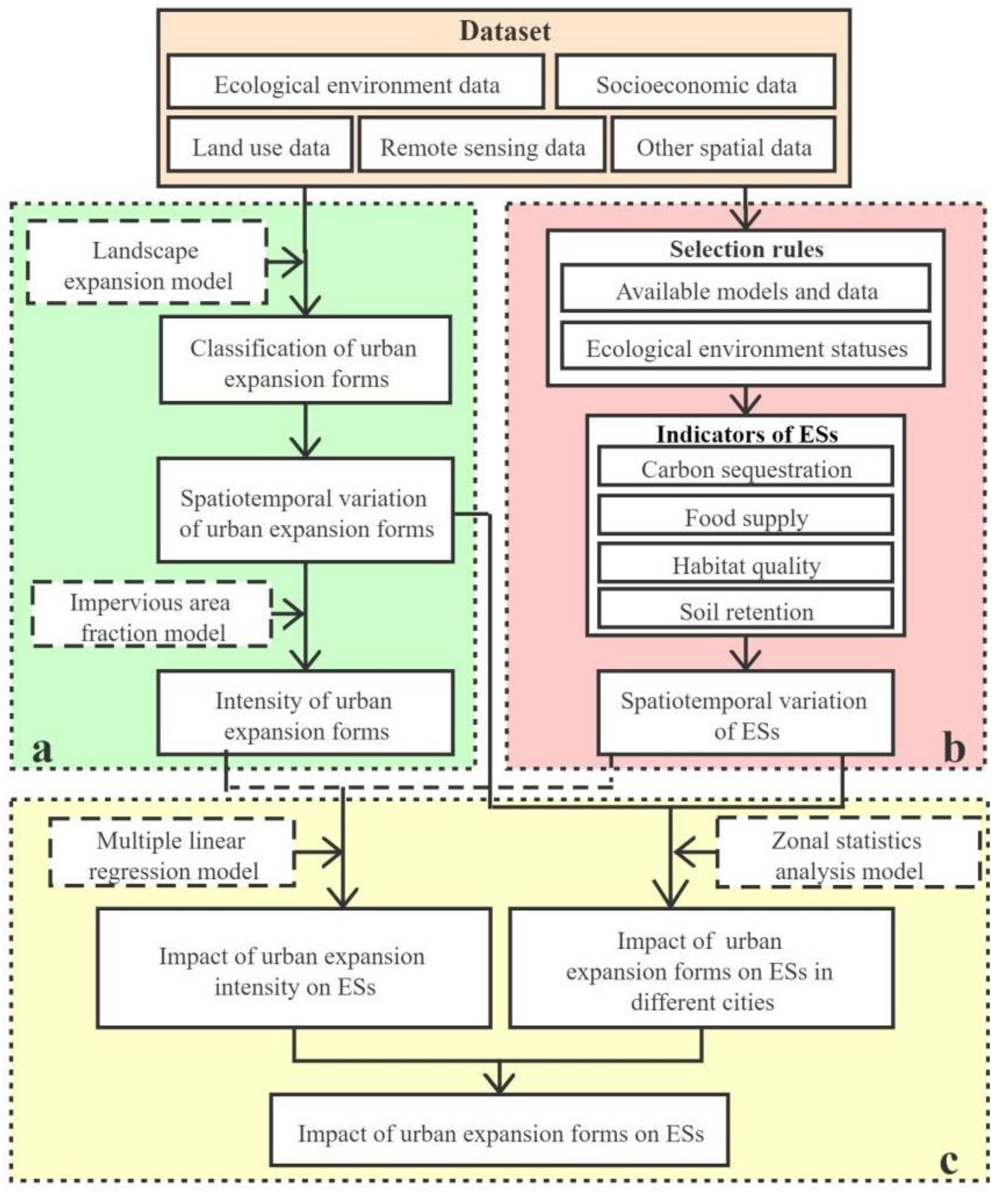
2. Materials and Methods

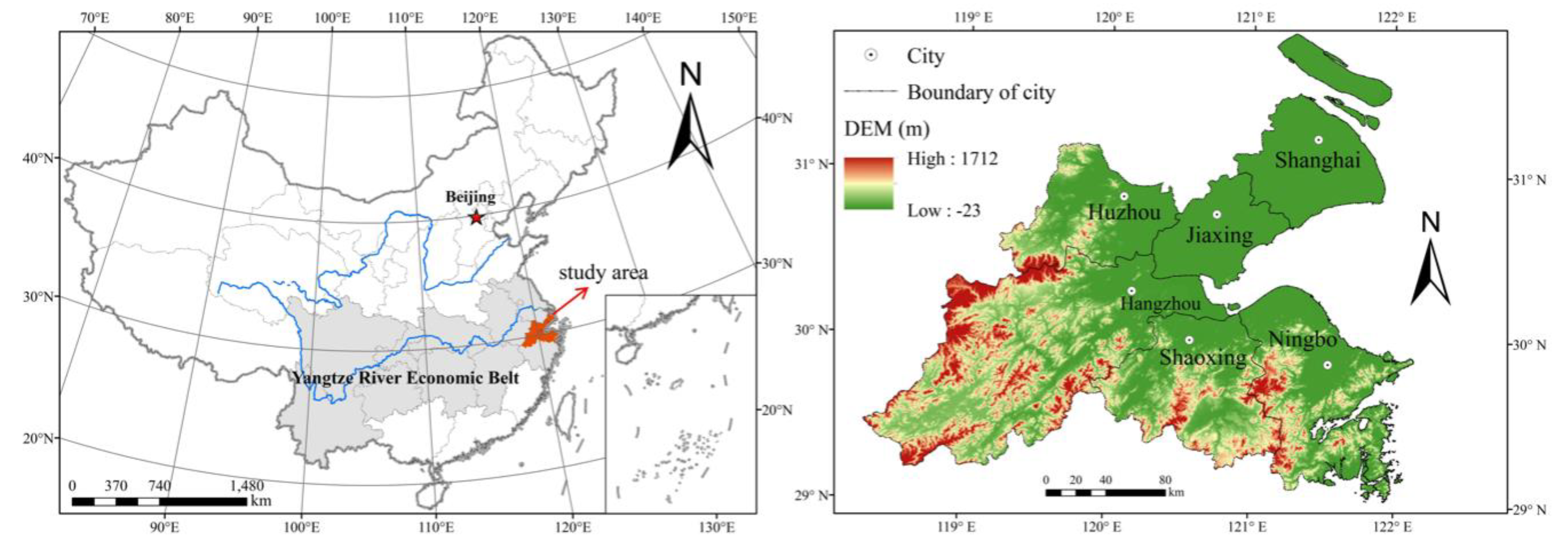
2.1. Study Area

The SHB, ranging from 118°21′ E to 122°16′ E and 28°51′ N to 31°53′ N, is located on the eastern coast of China and the lower reaches of the Yangtze River Basin, consisting of one core megacity, Shanghai, and five other cities (Hangzhou, Jiaxing, Shaoxing, Ningbo, and Huzhou) in Zhejiang Province (Figure 1). All boundaries were derived from the Standard Map Service System of the Ministry of Natural Resources of China in 2019 (http://bzdt.ch.mnr.gov.cn). SHB has many landform types, including plains, hills, basins, and plateaus. The elevation is higher in the west and lower in the east, and the annual rainfall is 1460 mm, while the average annual temperature is approximately 16 °C. In 1930s, the prototype of the urban agglomeration in SHB had already taken shape, and in recent decades, China’s reformation and opening up has made it an important growth pole for socioeconomic development in the Yangtze River Delta region. Especially after China’s reform and opening up, the proposal of a series of regional development strategies has significantly expanded the regional urban scales and accelerated the urban expansion pace. At the end of 2015, the total area of SHB had exceeded 50,000 km², with a total population exceeding 38 million, and the regional GDP was $769 million (USD). It is no doubt that SHB is one of the most important components of the world-class urban agglomeration in the Yangtze River Delta and one of the regions with the highest urbanization level in China. However, in recent years, with the population booming and economic inflation, rapid and large-scale urban expansion in SHB has resulted in fundamental changes in the function and structure of natural ecosystems, which in turn seriously threatens the sustainable development [39,40].

2.2. Data Source and Processing

In this study, Landsat 5 TM data with 30 m spatial resolution for 1990, 2000, and 2010, and Landsat 8 OLI data with 15 m spatial resolution for 2019 were used. All images were from June and July, collected from the GeospatialData Cloud of the Chinese Academy of Sciences (http://www.gscloud.cn). Based on ENVI 5.3 software, all remote sensing images were treated in advance by radiometric calibration and atmospheric correction to meet the requirements of our study. The Radiometric Calibration tool was used for the radiometric calibration, and the FLAASH Atmospheric Correction tool was applied for the atmospheric correction. All images that we obtained underwent geometric correction and were georeferenced, so we did not do these two steps.

Additionally, we obtained socioeconomic and ecological environment data for 1990, 2000, 2010, and 2019 from relevant government departments and resource data websites. For example, the socioeconomic data and grain production data were collected from the Zhejiang Provincial Bureau of Statistics and the Shanghai Bureau of Statistics; the cropland quality data were collected from the Zhejiang Provincial Department of Agriculture and the Shanghai Agriculture Bureau; the meteorological data were obtained from the Chinese meteorological data network (http://data.cma.cn), and they were interpolated through the inverse distance weighted method; and the soil type data were obtained from the Chinese Soil Database (http://vdb3.soil.csdb.cn).

The spatial geographic grid was proved to be an effective approach that could seamlessly link multi-scale geographical information to solve the problem of different data formats [11]. Thus, in order to accurately analyze the impact processes between urban expansion forms and ESs, we divided the study area into geographic grid cells of 1 km × 1 km.

The framework of our study is shown in Figure 2.

2.3. Mapping Land Use Cover

Based on the ENVI 5.3 software, the random forest (RF) classifier was used for land use cover classification in this study. RF is a machine learning method that can effectively process a large number of input indicators and provided fast and reliable classification results [41]. Compared with other remote sensing classifiers, the training speed of the RF classifier is faster and not prone to over-fitting [42]. Therefore, in current studies, the RF classifier is widely used in the map of land use cover [41,43,44].

2.3.1. Reference Dataset for Samples

Samples have a crucial impact on classification results [43]. Selecting representative samples for model training and accuracy evaluation of the RF classifier is an important prerequisite for ensuring the accuracy of land use cover. In this study, based on remote sensing images, referencing the sample point selection method of Zhang et al. [41], and combined with the Natural Resources Survey Map and the Google Image Map, 200 samples of each land use type were randomly selected via human–computer interactive extraction of remote sensing information for each year. The land use types were cropland, forestland, grassland, urban construction land, rural settlement, water bodies, and unutilized land.

Additionally, we randomly assigned a value from 0 to 1 for all samples. If a sample was less than 0.7, it was used as the training sample, otherwise it was the verification sample.

2.3.2. Remote Sensing Image Features and Classifier Parameters

To ensure the information contained in remote sensing images could be fully detected, we comprehensively considered various features as the training parameters of RF classifier, including the spectral characteristics of remote sensing images and the terrain features. For spectral characteristics, in addition to spectral bands of Landsat data (i.e., blue, green, red, near infrared, shortwave infrared 1, and shortwave infrared 2), the normalized difference vegetation index (NDVI) [45] and the enhancement vegetable index (EVI) [46] were used to distinguish vegetation from other land use types; the normalized difference build index (NDBI) [47] was applied to assist the monitoring of urban construction land and rural settlement; and the normalized difference water index (NDWI) [48] was used to detect water bodies. Simultaneously, topography greatly impacts the distribution of different land use types [49]. Therefore, we calculated the elevation and slope using DEM.

Combined with the related studies [41,42,43,44], the number of decision trees was set as 200, and default values were used for other parameters in the RF classifier.

2.3.3. Classification Accuracy Verification

The accuracy of land use cover mapping was assessed by the confusion matrix based on the validation samples for each period. The overall accuracy (OA), producer’s accuracy (PA), user’s accuracy (UA), and Kappa [50] were calculated for land use types, and these accuracy indices were showed in

Table 1. Accuracy indices for the reclassified classes in the four periods.

Year	Land Use Type	PA (%)	UA (%)	OA (%)	Kappa
1990	Cropland	81.08%	83.33%	85.71%	0.83
	Forestland	83.67%	85.42%
	Grassland	80.00%	83.33%
	Urban construction land	89.66%	92.86%
	Rural settlement	84.62%	81.48%
	Waters	88.46%	92.00%
	Unutilized land	78.26%	81.82%
2000	Cropland	81.25%	83.87%	86.67%	0.84
	Forestland	81.58%	81.58%
	Grassland	80.00%	82.76%
	Urban construction land	91.43%	94.12%
	Rural settlement	89.29%	86.21%
	Waters	91.67%	100.00%
	Unutilized land	88.00%	81.48%
2010	Cropland	80.00%	82.76%	86.19%	0.84
	Forestland	82.05%	84.21%
	Grassland	77.78%	81.46%
	Urban construction land	91.67%	94.29%
	Rural settlement	80.65%	83.33%
	Waters	92.59%	96.15%
	Unutilized land	87.50%	80.77%
2019	Cropland	82.76%	85.71%	89.05%	0.87
	Forestland	89.29%	86.21%
	Grassland	87.50%	84.00%
	Urban construction land	97.50%	95.12%
	Rural settlement	82.76%	85.71%
	Waters	93.33%	100.00%
	Unutilized land	81.25%	83.87%

. OA in 1990, 2000, 2010, and 2019 was 85.71%, 86.67%, 86.19%, and 89.05%, respectively, and Kappa in 1990, 2000, 2010, and 2019 was 0.83, 0.84, 0.84, and 0.87, respectively. These indices indicated the results of land use cover mapping was satisfactory and met the needs of the research.

Based on the division results of land use types, the spatial distributions of urban growth in SHB from 1990 to 2019 were obtained and served as an important basis for this study (Figure 3).

2.4. Mapping Urban Expansion Forms

2.4.1. Urban Expansion Index

Urban expansion is regarded as the most evident expression of land cover change. In this study, we used the landscape expansion index (LEI) to assess the urban expansion situations in SHB. LEI can identify the spatial expansion form of urban land by determining the spatial position relationship between existing urban land and new urban land [16,51], and it can be calculated by the landscape expansion model. Compared with the method that reflects the characteristics of urban land expansion in time series, LEI provides a more intuitive way of spatial expression, which can characterize the spatial process of urban land expansion [36]. It is calculated by the buffer area of the expanded plaque, and the equation is as follows:

$$LEI=\frac{A_0}{A_0+A_v}\times 100$$

(1)

where A₀ is the overlapping area between the buffer zone of the expanded patches and the original patches, A_v is the intersection between the buffer zone and the original patches. The value of LEI lies within [0,100].

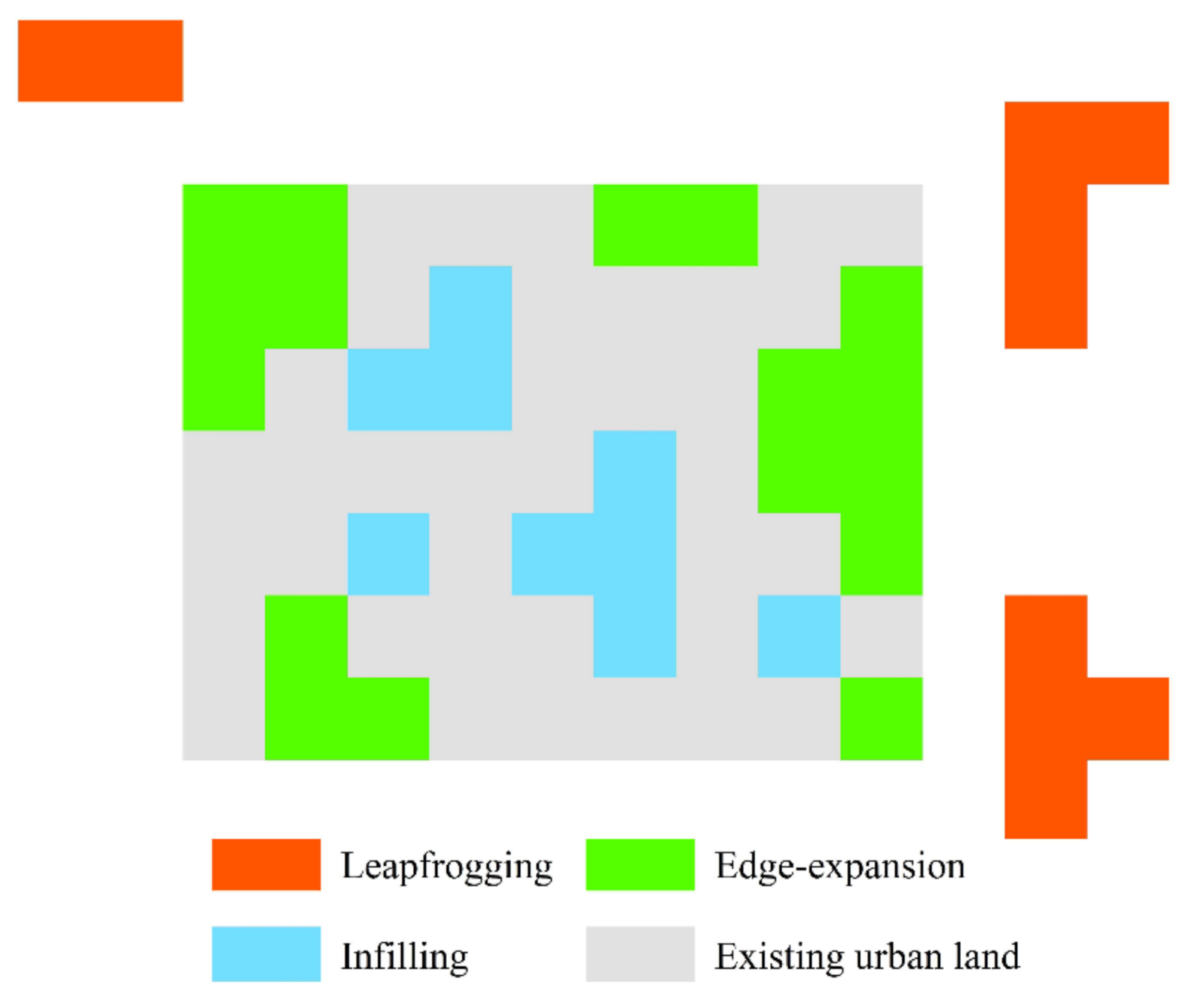
2.4.2. Classification of Urban Expansion Forms

Generally, the spatial expansion form of new urban land in a certain period can be divided into three categories: infilling, edge-expansion, and leapfrogging [51]. Among them, infilling indicates that urban expansion occurs in the internal blank area of the existing urban land; edge-expansion indicates the new urban areas extend outward along the edge of existing urban land; and leapfrogging indicates the new urban areas developed independently and without overlapping with any existing urban land [16]. The existence modes of these urban expansion forms are shown in Figure 4.

These urban expansion forms can be divided by LEI, and the classification criteria are fixed [16,36,51]. Based on previous studies, when LEI is 0, the expansion form is leapfrogging; when LEI is within (0, 50], the expansion form is edge-expansion; and when LEI is within (50,100], the expansion form is infilling.

2.4.3. Analysis of Urban Expansion Intensity

According to the definition of land use change intensity from land cover data, the urban expansion rate was used to analyze the urban expansion intensity in this study, which was defined as the trend of impervious area fraction (IAF) from 1978 to 2014 [52,53]. Furthermore, in order to more clearly explore the change state of urban expansion intensity in SHB, we focused on calculating the IAF for each geographic grid cell. The IAF is calculated as follows:

$$IAF=\frac{S_{Ui}}{S_{grid}}$$

(2)

where $S_{Ui}$ is the area of the i-th urban expansion type in a geographic grid cell, $S_{grid}$ is the area of a geographic grid cell. The value of IAF is within [0,100], a higher IAF indicates a higher urban expansion intensity in a specific grid.

The natural breaks method was used to divide the IAF of the three urban expansion forms into four levels: I, II, III, and IV. The higher the level, the stronger the intensity. This method can effectively prevent human subjectivity and classify similar values based on data distribution. However, we found that the natural breakpoint values in the three periods were slightly different in any expansion form, which might make the results incomparable. Therefore, to compare the structural changes and spatial changes of expansion intensity for the same urban expansion form, we adjusted the natural breakpoint values of IAF for the three urban expansion forms by using the arithmetic mean method and used the integers close to all of them as thresholds (

Table 2. The modified breakpoint values and natural breakpoint values for classifying the levels of urban expansion intensity.

Urban Expansion Form Type		Modified Value	Natural Breakpoint Value
			1990–2000	2000–2010	2010–2019
Leapfrogging	First breakpoint	8.00	7.28	9.10	7.90
	Second breakpoint	23.00	19.60	29.27	22.13
	Third breakpoint	49.00	48.70	52.81	45.56
Edge-expansion	First breakpoint	12.00	10.56	12.03	12.72
	Second breakpoint	37.00	34.02	36.41	40.48
	Third breakpoint	68.00	64.46	66.80	74.12
Infilling	First breakpoint	6.00	5.41	5.78	6.70
	Second breakpoint	21.00	19.78	19.56	22.89
	Third breakpoint	43.00	42.36	39.58	48.17

).

2.5. Quantifying Ecosystem Services

2.5.1. Selection of Ecosystem Service Types

Firstly, ES types that could be evaluated in this study should have the following characteristics: available models were used to quantify and map them, and basic data were easily obtained. Simultaneously, the specific selection of ESs types is critical to accurately characterize the status of the regional important ecosystems. Therefore, combining the regional ecosystem characteristics, the ecological environment statuses, and the relevant research in this region [39,54,55], our study focused on four ESs that were considered important and typical to SHB: carbon sequestration (CS), food supply (FS), habitat quality (HQ), and soil retention (SR).

2.5.2. Calculation of Ecosystem Services

Carbon Sequestration

CS is very important to the terrestrial carbon cycle, and it is the ability that the ecosystem has to absorb oxygen and release carbon dioxide. CS was chosen because it affects a wide variety of regulating services. Net primary production (NPP) was used as a proxy for CS, and it is an important factor for determining ecosystem carbon sources/sinks and regulating ecological processes [56]. Hence, we estimated CS of our study area based on NPP, which is mainly summarized in the following equation:

$$CS=\alpha \times \beta \times {\displaystyle \sum NPP}$$

(3)

where $\alpha$ is the proportion of carbon in carbon dioxide, which is 27.27%; $\beta$ is the carbon dioxide for every 1 g of dry matter in vegetation, which is 1.63 g [56]. NPP was calculated by using CASA model according to Wang et al. [13].

Food Supply

FS is crucial for food security and urban sustainability, and it is the ability that the ecosystem has to produce food and related products. In general, FS can be represented by the total grain output [57]. Because the total grain output is the statistical data, FS obtained represents the planar element results, and FS cannot be calculated for each grid in the study area. The results obtained by relying on the total grain output alone cannot meet our need to accurately assess the impact of urban expansion forms on FS. Some studies have shown a significant linear correlation between grain output and NDVI [57,58,59], and the researchers obtained the spatial distribution of FS through the combination of NDVI and CSum.

In this study, the grain output related to cropland was equally assigned to cropland in every county and then combined with the NDVI of cropland in each county to calculate FS for each grid in SHB. The equation is as follows:

$$FS=\frac{NDV{I}_i}{NDV{I}_{sum}}\times C_{sum}$$

(4)

where $NDV{I}_i$ is the NDVI of the i-th grid, $NDV{I}_{sum}$ is the sum of the NDVI of cropland in each county, $C_{sum}$ is the total grain output in each county.

Habitat Quality

HQ plays an essential role in organism dispersal among habitat patches and, thus, in conserving biodiversity, and it is the ability that the ecosystem has to provide suitable conditions for biological survival [60]. Considering the same habitat has different abilities to provide ESs for species in different regions, the vegetation coverage was used as an expression of habitat productivity to assess HQ [61], and the equation is:

$$HQ=Q_1+Q_2$$

(5)

where $Q_1$ is the NDVI, $Q_2$ is the value of HQ assessed by the InVEST model [62,63], which uses a half saturation curve equation to calculate the HQ score:

$$Q_2=H_{xj}\times (1-\frac{D_{xj}^z}{D_{xj}^z+k^z})$$

(6)

where H_xj is the habitat suitability score of landscape type j in grid cell x; k is a half saturation constant, which is customized according to the resolution of the data resource; z is a scale constant that reflects spatial heterogeneity; D_xj indicates the total threat level in grid cell x with landscape type j, and the equation is:

$$D_{xj}={\displaystyle \sum _{r=1}^R{\displaystyle \sum _{y=1}^{Y_r}(w_r/{\displaystyle \sum _{r=1}^R{w}_r})}}{r}_y{i}_{rxy}{A}_x{S}_{jr}$$

(7)

where R is the number of threat factors; Y_r is the set of grid cells on r’s raster map; w_r is the impact weight of threat factor r; A_x is the accessible grid x; S_jr indicates the relative sensitivity of landscape type j to threat factor r—the value is 0–1; i_rxy is the impact distance of threat factor r, which can be divided into linear or exponential function of distance from threats to habitats [49].

Identifying threats to habitats is a key issue for the assessment of HQ in the InVEST model. According to the actual local situation and some other studies [55,61], cropland, urban construction land, rural settlement, airports and port land areas, railways, and main roads were taken as threat factors. Simultaneously, combined with our previous research [61], the related coefficients of these threat factors were set (

Table 3. The threat factors and related coefficients.

Threat Factor	dr_max (km)	Weight wr	Distance-Decay Function
Cropland	5	0.5	Exponential
Urban construction land	12	1	Exponential
Rural settlement	7	0.8	Exponential
Airport and port land	10	0.8	Exponential
Railway	9	0.8	Linear
Main road	10	1	Linear

).

In addition, the habitat suitability scores of nine land use types were determined by referencing the InVEST user guide [62] and a previous study [64]. The habitat suitability of forestland was defined as 1 due to the persistence of individuals and groups of organisms [64]. For others, water bodies, grassland, cropland, and other land use types, values were 0.9, 0.8, 0.6, and 0, respectively.

Soil Retention

SR is an important regulating ecosystem service, especially under conditions of urban population growth and increasing areas of gray infrastructure in China, and it is the ability that each plot in the ecosystem has to maintain soil. Areas of land with high SR have the capacity to alleviate a series of ecological disasters caused by human over-development, such as floods and mudslides. The revised universal soil loss equation model (RUSLE) [65] can be used to measure SR, and the equation is as follows:

$$SR=RKLS-USLE=R\times K\times LS-R\times K\times LS\times C\times P$$

(8)

where RKLS is the potential for soil loss, USLE is the annual soil loss; R is the rainfall erosion factor, K is the soil erodibility factor, LS is the slope length and steepness factor, C is the cover and management factor, P is the conservation practice factor. The calculation method of each coefficient is presented in Asadolahi [65].

2.6. Analysis of Interactive Coercing Relationships

2.6.1. Multiple Linear Regression Model

Based on the analysis of the dynamics of the expansion intensity for different urban expansion forms and ESs in SHB from 1990 to 2019, the relationship between the expansion intensity of different expansion forms and ESs was shown by using the multiple linear regression (MLR) model, which is the most commonly used model for analyzing the linear relationship between two or more variables [61]. In this study, the changes of four ESs in 1990–2000, 2000–2010, and 2010–2019 were selected as the dependent variables, and the expansion intensities of various urban expansion forms were chosen as the independent variables. The MLR model can be expressed as follows:

$$y_i={\beta }_0+{\displaystyle \sum _{k=1}^i{\beta }_k{x}_k+\epsilon }$$

(9)

where $y_i$ is the change value of ESs, $x_k$ is the expansion intensity of different expansion forms, $k$ is the total number of spatial units involved in the analysis, ${\epsilon }_{}$ is the random error term that follows an independent normal distribution with a mean of 0, ${\beta }_0$ is the constant term estimate, and ${\beta }_k$ is the k-th regression parameter, which is a function of geographic location.

2.6.2. Zonal Statistics Analysis Model

According to the Chinese city level classification standard, all cities in SHB were divided into four levels: mega-scale city (Shanghai), large-scale city (Hangzhou), medium-scale city (Ningbo, Jiaxing, and Shaoxin), and small-scale city (Huzhou). The higher the urban level, the larger the urban size.

In this study, the zonal statistics analysis (ZSA) model was selected to explore the impact of urban expansion forms on ESs in different cities. The ZSA model is based on the partition statistical functions, takes the classification areas of one data set as the statistical units to count the unit values at the corresponding position in another data set, and can intuitively reflect the development of another attribute in a classification area [15]. In this model, the changes of four ESs were taken as the statistical objects, and the geographic grid cells of various urban expansion forms in different cities were taken as the statistical zones.

3. Results

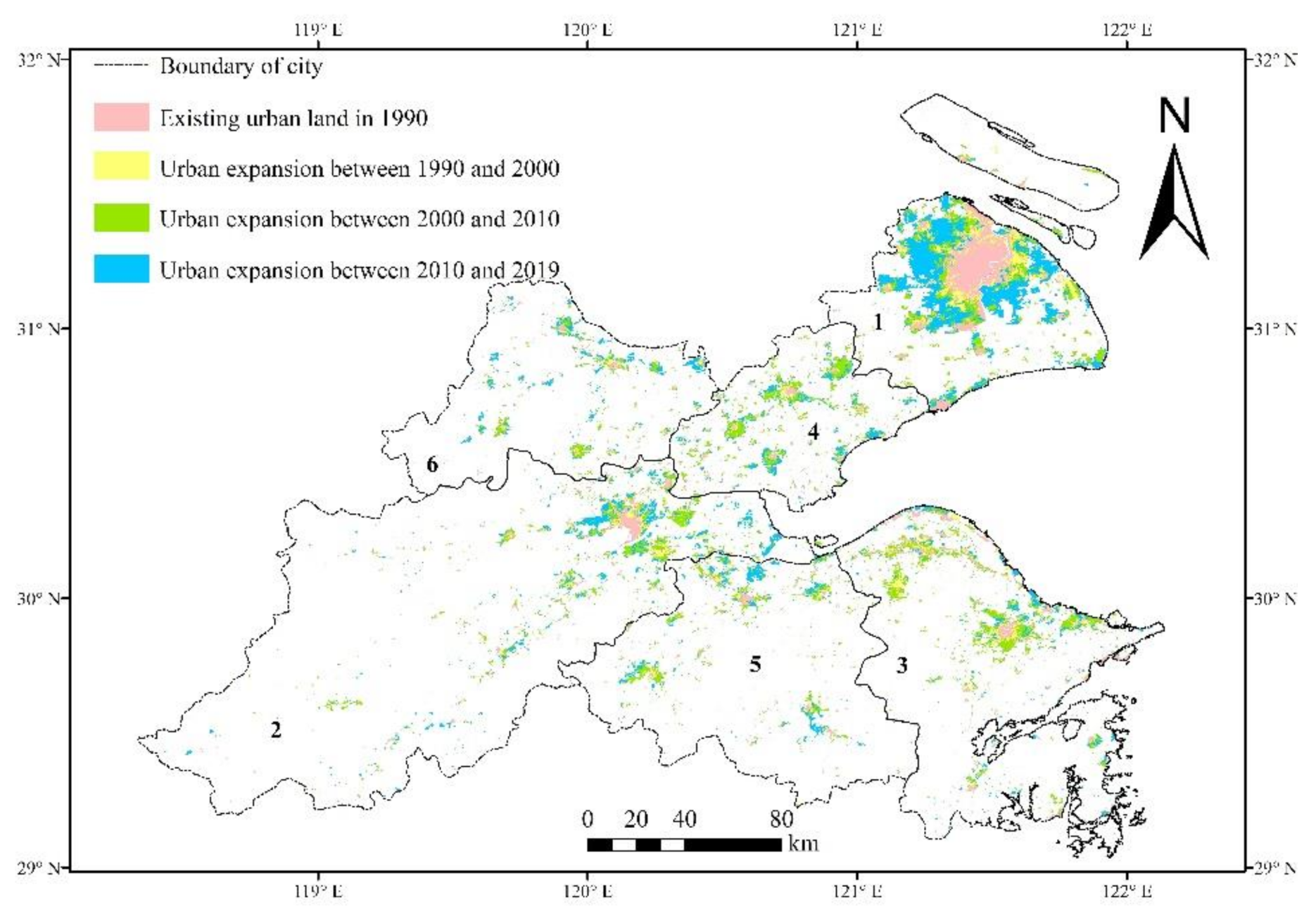
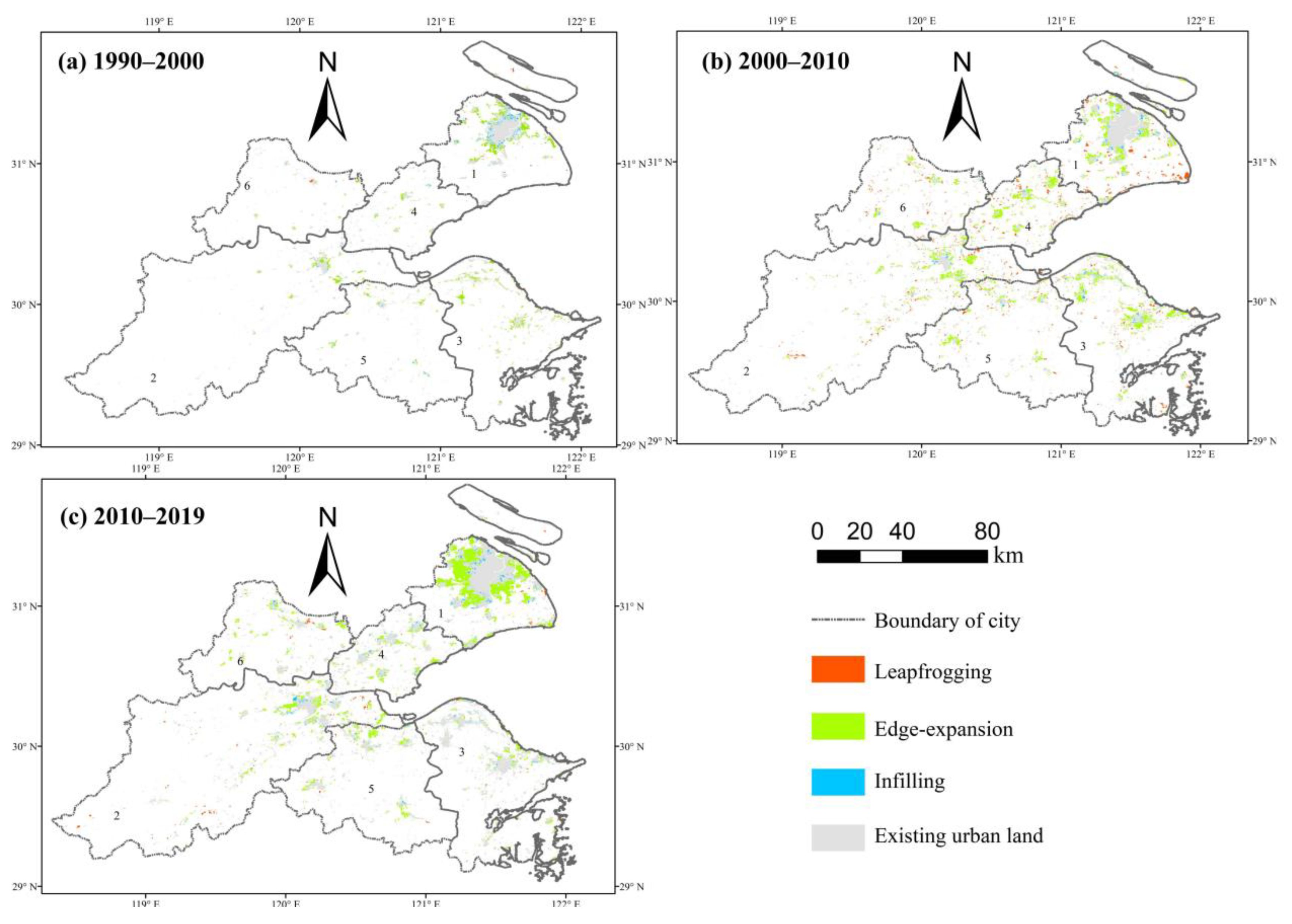
3.1. Spatiotemporal Variation of Urban Expansion Forms

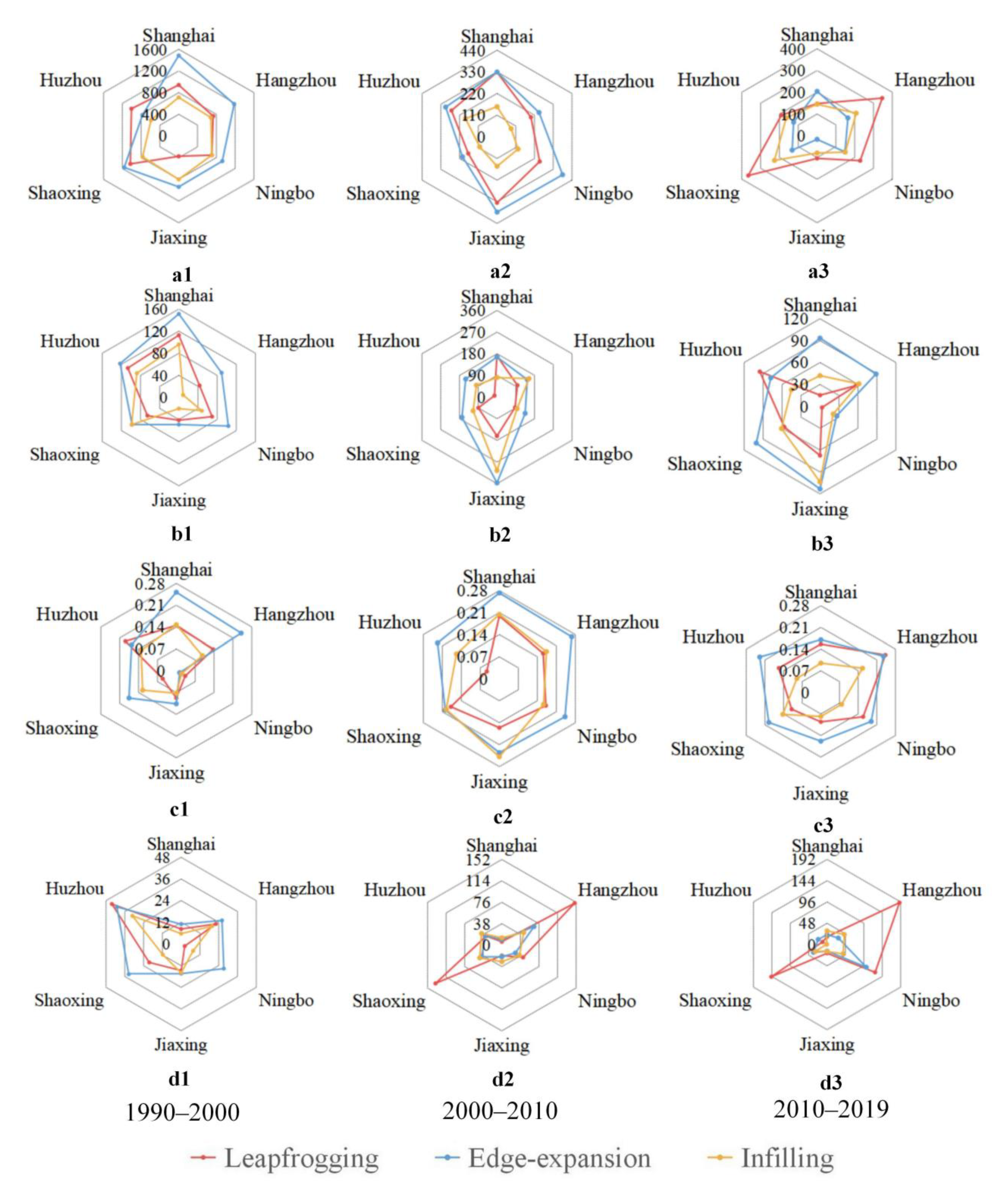
3.1.1. Growth Change of Urban Expansion Forms

Figure 5 shows the compositions of urban expansion forms for different cities in SHB. The results showed that the dominant form of urban expansion was edge-expansion from 1990 to 2019, and the proportion of leapfrogging experienced a substantial increase in the process of urban growth. In detail, in 1990–2000, edge-expansion was the dominant form of urban expansion, reflecting that the urban structure was inseparable in this period; in 2000–2010, the area and patch proportion of leapfrogging demonstrated an upward trend, especially in Ningbo, Jiaxing, and Huzhou, it surpassed the proportion of the edge-expansion; and in the last period, the edge-expansion once again dominated the urban expansion direction. These changes indicated that the urban expansion trend in SHB experienced a morphological change from integration to diffusion, and finally to integration.

Figure 6 clearly describs the spatial evolution processes of various urban expansion forms among three neighboring periods for these newly developed urban land patches. In 1990–2000, the leapfrogging, edge-expansion, and infilling could be found in the whole area, and their changes in Shanghai, Hangzhou, Jiaxing, and Ningbo were the most obvious. Among of them, edge-expansion was the main expansion form and was mainly distributed in the center, east, and northeast. Furthermore, many urban land patches in the infilling were largely within the core of the northeastern municipal district (i.e., Shanghai). In 2000–2010, the edge-expansion had many distributions and occurred around the existing urban land, and the main distribution areas were similar to the previous stage. Simultaneously, many considerable urban land patches in the leapfrogging appeared on the east coast, the northeast coast, and the north plain, but they mainly showed distribution patterns with a dominant number of small-sized patches. In 2010–2019, the edge-expansion scale around the existing urban land greatly increased in the center and northeast, nd the scope of the leapfrogging patches also increased in the core areas of the socioeconomic development in the whole of SHB (i.e., Shanghai and Hangzhou).

3.1.2. Intensity Change of Urban Expansion Forms

Based on the calculation of IAF for SHB from 1990–2000, 2000–2010, and 2010–2019, the expansion intensities of various urban expansion forms were obtained. The results showed that the I level of expansion intensity was the dominant interval, and the proportion of I was higher than 60% in the whole period. However, the various intensity levels of different expansion forms changed significantly with the expansion of urban scales (

Table 4. The proportion of urban expansion intensity levels for different urban expansion forms from 1990 to 2019 (%).

Urban Expansion Form Type	Time Interval	Urban Expansion Intensity Level
		I	II	III	IV
Leapfrogging	1990–2000	80.84	14.36	3.27	1.53
	2000–2010	63.77	24.06	8.71	3.46
	2010–2019	60.36	24.99	9.02	5.63
Edge-expansion	1990–2000	77.52	11.47	7.00	4.01
	2000–2010	71.49	13.11	8.49	6.91
	2010–2019	78.16	8.12	5.48	8.24
Infilling	1990–2000	77.78	13.94	5.55	2.73
	2000–2010	93.74	3.27	1.64	1.35
	2010–2019	94.73	3.05	1.49	0.73

and Figure 7). For the leapfrogging, the proportion for II, III, and IV kept increasing, and II increased the most, which was 10.63%, followed by III; for the edge-expansion, different intensity levels had different development trends, among which IV kept increasing, which increased by 4.23% from 1990 to 2019; and for the infilling, the proportion of I increased continuously in the whole period, but other levels had the opposite trend.

In terms of the spatial distribution of expansion intensity, the high intensity area of leapfrogging was mainly distributed in the northeast in 1990–2000, and there were a considerable number of growth points in the central region in 2000–2010, but the distribution area greatly shrunk after 2010. The northeast of SHB had always been the distribution area of the high intensity area for the edge-expansion, which gradually expanded year by year, and the central and east of SHB exhibited numerous high-intensity areas after 2000. The high intensity area of the infilling was mainly distributed in the northeast during the whole period, and after 2000, there were sporadic growth points in the central and east, but their scopes were limited.

3.2. Spatiotemporal Variation of Ecosystem Services

3.2.1. Temporal Variation of Ecosystem Services

In the temporal changes of ESs, the maximum annual average change rates of CS, FS, HQ, and SR in 1990–2000, 2010–2019, 2000–2010, and 2010–2019 were −2.16%, −3.38%, −0.42%, and −3.22%, respectively (

Table 5. Change rates of ESs in SHB from 1990 to 2019 (%).

City	CS			FS			HQ			SR
	1990–2000	2000–2010	2010–2019	1990–2000	2000–2010	2010–2019	1990–2000	2000–2010	2010–2019	1990–2000	2000–2010	2010–2019
Shanghai	−19.44	−12.03	13.53	−28.43	−32.31	−11.67	−1.44	−16.15	−11.13	13.02	−0.85	7.96
Hangzhou	−19.49	−1.38	21.67	−18.23	−34.93	−50.42	2.65	−1.85	−1.42	−2.58	20.07	−42.34
Jiaxing	−14.51	−9.74	15.42	0.00	−40.87	−30.41	−0.07	−10.45	−5.99	−9.27	25.31	6.97
Huzhou	−19.00	1.26	17.97	−29.82	−5.32	−42.52	2.16	−1.96	−2.42	−0.96	18.98	−22.06
Ningbo	−22.09	−3.96	19.58	−28.57	−34.76	−23.03	1.41	−5.53	−1.60	8.57	4.54	−20.08
Shaoxing	−22.20	2.03	22.73	−21.84	−19.57	−46.94	2.03	−2.35	−1.38	8.66	15.03	−32.65

). In terms of different cities, CS in Shanghai experienced the greatest decrease from 1990 to 2019, which was −19.54%; the maximum change rate of FS in 1990–2000 was in Huzhou, in 2000–2010 was in Jiaxing, and in 2010–2019, was in Hangzhou, which was −29.82%, −40.87%, and −50.42%, respectively; HQ in Hangzhou, Huzhou, Ningbo, and Shaoxing increased in 1990–2000, but all cities showed downward trends in the latter two periods (among them, Shanghai dropped consistently the most, i.e., −16.15% and −11.13% respectively), and the greatest change in SR in 1990–2000, 2000–2010, and 2010–2019 was distributed separately in Shanghai, Jiaxing, and Hangzhou, i.e., 13.02%, 25.31%, and −42.34%, respectively.

3.2.2. Spatial Variation of Ecosystem Services

As shown in Figure 8, there were significance differences in the spatial distribution of the change trend for the four ESs. (1) CS showed spatial heterogeneity with an increasing trend from the northeast to the south and southwest (Figure 8a). In 1990–2000, the CS in the whole SHB increased, while it presented a reduction around the urban land in the northwest and central (especially in Shanghai and Hangzhou); in 2000–2010, the increased areas were mainly distributed in the south and west (i.e., Shaoxing and Huzhou), while the decreased areas were concentrated in Jiaxing and Shanghai in the northeast; and in 2010–2019, the increased areas were the same as in the previous stage, but the decreased areas were mainly distributed in Hangzhou, Huzhou, and Shanghai in the central and northeast. (2) The high value areas of FS were mainly distributed in plain regions in the central and northeast, with relatively low values in other regions (Figure 8b). In the spatial change, the increased areas were extremely small from 1990 to 2019, which were mainly distributed in coastal areas in the east and northeast, and the decreased areas were mainly distributed in Jiaxing in the northeast and Shaoxing in the south, and Jiaxing had the most obvious decrease in 2000–2010. (3) The high and low values of HQ were spatially staggered, which had a downward trend from the southwest to the northeast (Figure 8c). In the spatial change, the decreased regions far exceeded that of increased regions, and the former were mainly distributed in Hangzhou in the central, Ningbo in the east, and Shanghai in the northeast. (4) The spatial distribution differentiation of high and low values for SR was the same as that for HQ (Figure 8d). In the spatial change, the areas of increase and decrease were mainly distributed in the mountain and basin areas in the south, southwest, and southeast. Among them, from 1990 to 2010, the increased areas were concentrated in Hangzhou, Shaoxing, and Ningbo, and in 2010–2019, they were mainly distributed in Ningbo.

3.3. Correlations between Urban Expansion Forms and Ecosystem Services

3.3.1. Impact of Urban Expansion Intensity on ESs

The expansion intensity for various urban expansion forms influenced the changes of ESs, but their influence degrees were not the same.

We used Pearson correlation via SPSS 22.0 to conduct the correlation analysis between expansion intensity of urban expansion forms and ESs. The results indicated that the correlation coefficients in different periods all passed the significance test.

Therefore, to compare the impact degrees of expansion intensity for various urban expansion forms that affected the changes in ESs, the MLR model was applied to quantify the impact of expansion intensity of urban expansion forms on ESs.

Table 6. The variance analysis results of the MLR model for the expansion intensity of urban expansion forms and the change in CS in different time intervals.

Time Interval	Urban Expansion Form	Indexes
		Coefficient	Std. Error	t-Statistic	VIF	R2	R2 Adjusted
1990–2000	Leapfrogging	−0.523 **	0.084	−37.036	2.356	0.752	0.747
	Edge-expansion	−0.732 **	0.126	−3.370	1.759
	Infilling	−0.067 *	0.193	−6.581	3.213
2000–2010	Leapfrogging	−0.559 **	0.164	−23.895	1.998	0.775	0.772
	Edge-expansion	−0.654 **	0.089	−36.554	3.467
	Infilling	−0.281 **	0.472	−5.949	1.265
2010–2019	Leapfrogging	−0.549 **	0.369	−24.882	1.659	0.757	0.741
	Edge-expansion	−0.399 **	0.082	−18.679	2.356
	Infilling	−0.176 **	0.473	−12.901	1.147

Note: ** and * represent the passing of 1% and 5% significance levels, respectively.

,

Table 7. The variance analysis results of the MLR model for the expansion intensity of urban expansion forms and the change in FS in different time intervals.

Time Interval	Urban Expansion Form	Indexes
		Coefficient	Std. Error	t-Statistic	VIF	R2	R2 Adjusted
1990–2000	Leapfrogging	−0.532 **	0.457	−4.235	1.989	0.875	0.847
	Edge-expansion	−0.693 **	0.095	−17.574	1.453
	Infilling	−0.283 **	0.342	−3.409	2.658
2000–2010	Leapfrogging	−0.567 **	0.105	−23.615	2.659	0.761	0.753
	Edge-expansion	−0.718 **	0.057	−15.726	1.863
	Infilling	−0.181 **	0.303	−3.888	3.549
2010–2019	Leapfrogging	−0.311 **	0.114	−4.264	2.351	0.796	0.791
	Edge-expansion	−0.579 **	0.025	−19.418	5.681
	Infilling	−0.226 **	0.146	−2.717	1.768

Note: ** and * represent the passing of 1% and 5% significance levels, respectively.

,

Table 8. The variance analysis results of the MLR model for the expansion intensity of urban expansion forms and the change in HQ in different time intervals.

Time Interval	Urban Expansion Form	Indexes
		Coefficient	Std. Error	t-Statistic	VIF	R2	R2 Adjusted
1990–2000	Leapfrogging	−0.389 **	0.035	−13.725	1.847	0.672	0.659
	Edge-expansion	−0.464 **	0.024	−9.512	1.375
	Infilling	−0.165 **	0.179	−6.757	4.269
2000–2010	Leapfrogging	−0.433 **	0.057	−27.964	1.357	0.731	0.718
	Edge-expansion	−0.392 **	0.131	−16.486	1.188
	Infilling	−0.245 **	0.016	−7.410	2.019
2010–2019	Leapfrogging	−0.487 **	0.103	−17.084	2.086	0.826	0.809
	Edge-expansion	−0.258 **	0.023	−42.210	1.741
	Infilling	−0.346 **	0.133	−6.121	1.057

Note: ** and * represent the passing of 1% and 5% significance levels, respectively.

and

Table 9. The variance analysis results of the MLR model for the expansion intensity of urban expansion forms and the change in SR in different time intervals.

Time Interval	Urban Expansion Form	Indexes
		Coefficient	Std. Error	t-Statistic	VIF	R2	R2 Adjusted
1990–2000	Leapfrogging	−0.487 **	0.118	−11.181	4.073	0.773	0.758
	Edge-expansion	−0.419 **	0.089	−7.258	2.964
	Infilling	−0.042 *	0.142	−3.199	1.786
2000–2010	Leapfrogging	−0.577 **	0.330	−2.337	3.659	0.803	0.793
	Edge-expansion	−0.392 **	0.178	−11.714	1.178
	Infilling	−0.381 **	0.947	−4.026	1.382
2010–2019	Leapfrogging	−0.638 **	0.902	−1.633	2.937	0.795	0.799
	Edge-expansion	−0.258 **	0.201	−12.801	5.005
	Infilling	−0.205 **	0.156	−3.881	1.686

Note: ** and * represent the passing of 1% and 5% significance levels, respectively.

show the variance analysis results of the MLR model in different time intervals. The fitting results of the MLR model indicated the following characteristics: all regression coefficients passed the 1% or 5% significant level test, and all VIF values were smaller than 7.5, showing that there was no variable redundancy in the model, and there was no multiple linear relationship among these urban expansion forms.

The results of the MLR model showed that the expansion intensities for the leapfrogging, edge-expansion, and infilling all had significant negative impacts on ESs, but these negative influences changed significantly with the development of the cities. (1) For CS, before 2010, the increase in the edge-expansion intensity brought the most losses of CS, and in 2010–2019, the increase of the leapfrogging intensity had the greatest impact on CS (Table 6). (2) For FS, the edge-expansion intensity had the greatest negative impact, followed by the leapfrogging intensity. The coefficients of the edge-expansion intensity experienced fluctuating changes, which were −0.693 **, −0.718 **, and −0.479 ** (Table 7). (3) For HQ, in 1990–2000, the edge-expansion intensity had the greatest negative impact, and after 2000, the greatest negative impact was produced by the leapfrogging intensity. Additionally, the negative impact of edge-expansion intensity gradually decreased, eventually reaching −0.258 **; but the negative impact of leapfrogging intensity gradually increased, eventually reaching −0.487 ** (Table 8). (4) For SR, the leapfrogging intensity had the greatest negative impact in the whole period, and the coefficient gradually decreased in 1990–2000, 2000–2010, and 2010–2019, which was −0.487 **, −0.577 **, and −0.638 **, respectively (Table 9).

3.3.2. Impact of Urban Expansion Forms on ESs in Different Cities

The impact of urban expansion forms on ESs in different cities had regional differences (Figure 9).

In the early expansion (1990–2000), the edge-expansion in Shanghai had the greatest negative impact on CS, FS, and HQ, which was 672.60 kgC/km², 137.12 kg/km², and 0.25, respectively, and the negative impact of the leapfrogging in Huzhou on SR was the greatest, which was 44.27 t/km². With the expansion of urban scales, the relationship between urban expansion forms in different cities and ESs underwent tremendous transformations after 2000. For CS, the negative influence of urban expansion forms decreased year by year, and in 2010–2019, the greatest negative impact appeared in the leapfrogging, which was 365.59 kg C/km² in Sahaoxing. For FS, the edge-expansion always had the greatest negative influence and appeared in Jiaxing. However, during the period 2000–2010 and 2010–2019, it first increased and then decreased and was 356.84 and 113.29 kg/km² respectively. For HQ, in 2000–2010, the edge-expansion in all cities had the greatest negative impact; among them, Shanghai was the largest, which was 0.27, and in 2010–2019, the greatest negative impact appeared in the edge-expansion in Huzhou, which was 0.24, but for Shanghai and Hangzhou, the leapfrogging had the greatest effect, which was 0.20 and 0.22, respectively. For SR, the negative impact of various cities increased, and the greatest influence appeared in the leapfrogging in Hangzhou.

4. Discussion

4.1. The Relationship between Urban Expansion Forms and ESs

Urban expansion is one of the most intuitive manifestations of urbanization development [66]. There is no doubt that the changes in ESs are closely related to urban expansion. Urban expansion occupies a large amount of high-quality arable land and beautiful ecological land [67,68,69], destroys the agricultural farming environment and natural ecological environment, and affects the original stable landform type structure during the expansion process [17]. Therefore, reveling the impact of urban expansion forms on ESs provides an important basis to maintain the sustainable development of urban ecosystems.

In this study, we deeply revealed the relationship between various urban expansion forms and ESs and their specific influential mechanisms. The results showed that urban expansion had negative effects on the original functions of the ecosystem to varying degrees, but the losses of ESs resulting from the development of urban expansion forms may be phased. In the early expansion, the closer to the original city, the greater potential for urban construction [70]. However, because these areas are close to residential areas, there are many human activities, which pose huge threats to the security and stability of the ecosystem and cause ESs to decline [68]. Meanwhile, in the fringe areas of the cities, urban expansion has also brought about a series of different influences, e.g., the rise of facility agriculture, the agricultural non-point source pollution caused by the widespread use of chemical fertilizers and pesticides, and the large amounts of industrial wastewater generated by the rapid development of industry. They will cause the deterioration and imbalance of the water and soil environment in the urban expansion regions [20,23]. Therefore, in general, in the early expansion, the edge-expansion had the greatest negative impact on ESs.

After China’s reform and opening up, the speed of urban expansion in China has increased rapidly, especially in urban agglomerations such as SHB [54,55]. The infilling and edge-expansion have expanded the scope of the core area for each city, and the city size has increased significantly. The process reverses the previous relationship between urban expansion forms and ESs. The result is consistent with previous studies [30,71]. Compared to the large-scale urban zones, the small-scale urban zones had more significant negative impacts on the most types of ESs, and the negative influences produced by various expansion forms in the former showed a decrease trend year by year. Especially in SR, this characteristic was very obvious. Calzolari’s study also demonstrated the unsealed soils in the areas with concentrated development of construction land had higher SR than in the areas with less urban development [72]. Thus, as shown in Table 6, Table 8 and Table 9, the negative impact of leapfrogging on ESs was greater than that of edge-expansion and infilling. Simultaneously, for the large-scale urban zones, many studies indicated that with the expansion of urban scales, urban land in this region experienced more greening than in other sized cities through urban land use management and related land remediation projects (e.g., the urban large garden construction), which improved the internal ecosystem and enhanced the sustainability of urban development [6,36,73].

Additionally, we found that the edge-expansion always had the greatest negative impact on FS, but this impact varied during the expansion stages. Due to the agglomeration effect of resources in urban areas, there are many high-quality cropland resources distributed around the cities [74]. However, a study found that obvious cropland losses always emerged in cities with high administrative levels and large population sizes, and the acceleration stage of croplands losses always appeared earlier in cities with high administrative levels and a large city scale [75]. Thus, the greatest negative impact of urban expansion first appeared in the large-scale and high-level cities. Compared to leapfrogging and infilling, edge-expansion will inevitably occupy more high-quality cropland, eventually leading to a large reduction in FS.

4.2. Implications for Ecological Environment Improvement in Urban Agglomerations

In the future development, the population’s demand for urban land will continue to increase, and the urban scale will continue to show a trend of rapid expansion. Improving the effectiveness of ES protection is conductive to achieve coordination between urban expansion and the ecological environment. Therefore, it is indispensable to make targeted recommendations in the context of new urbanization based on the impact mechanism of urban expansion forms and ESs.

In the areas where the cropland has a high concentration and high quality, to reduce the pressure of the loss of FS, the encroachment of urban areas on cropland should be strictly controlled by restricting the amount and intensity of urban expansion. Then, under the premise of rationally setting the urban expansion boundaries, urban expansion should be dominated by leapfrogging and infilling. The edge-expansion should adopt the small-scale and refined development as the main direction of urban expansion, which will avoid the occupation of high-quality cropland to the greatest extent. For the areas with high internal density in the urban space and many external restrictions, integrating occupied land and intensively using existing construction land will help maintain the ecosystem stability [25], and replacing simple horizontal expansion with urban vertical development is also an effective urban development method [76]. In addition, although the existing studies have shown that the increase in the population density in the contiguous areas where arable land is concentrated can effectively improve FS in the rural areas [77], in urban agglomerations, the population density still needs to be controlled, which can reduce the population’s demand for food and ease the pressure on FS [78].

In the areas with a good ecological environment, the sporadic distribution of urban areas can interfere with the connectivity of ecological landscape types [72]. Many studies have found that the impact of urban form compactness on ecosystem health is very evident in the process of urban development, and a compact and continuous urban form can improve the stability of ecosystem structure and maintain the sustainable health of ecosystems [61,79]. To maintain the stability of the ESs and improve the value of ESs, edge-expansion and infilling should be the dominant urban expansion forms. It is obvious that the land use types occupied by urban expansion in these regions are mainly forestland, grassland, and a small amount of cropland. Protecting ecosystem types with high ecosystem service value is one of the effective ways to improve ESs [80]. It is very important to scientifically delineate the ecological protection red line areas and implement strict protection. Existing studies have shown that in the urban expansion process, ESs seem to have a greater negative impact on one-way land transfer rather than on two-way land transfer [77]. Therefore, expanding the scope of “blue–green spaces” within cities is also one of the effective ways to maintain and stabilize ESs [76]. It not only helps alleviate the pressure of urban expansion on the regional ecosystem, but also protects the original ecological state and the ecosystem integrity.

4.3. Limitation and Future Directions

Based on the exploration of the spatiotemporal dynamic evolution of urban expansion forms and the relationship with ESs, this study revealed the impact process of urban expansion on ESs. The research results can provide important information for ES improvement and the urban development planning in various urban expansion regions, but still have limitations.

As described in the previous content, urban expansion is a double-edged sword. While it brings losses of ESs, it also has a positive effect on some ESs. For example, for FS, as the rate of regional urbanization increases, the scope of facility agriculture will gradually expand [81], and the factory production of agriculture will become the inevitable result of the agricultural development in urban expansion areas [82]. These factors will result in the increase in FS. However, the maximum remote sensing image resolution that can be obtained by this research is 15 m, which cannot accurately divide cropland and facility agricultural land. Moreover, because of the limitation of data access, we do not have the necessary data to effectively evaluate the state of factory production of agriculture. In future research, we will carry out more in-depth explorations in these aspects.

5. Conclusions

In recent years, revealing the impact of urban expansion on ecosystem has gradually become a hot topic. However, analyzing their relationships from the perspective of different urban expansion forms is very limited, which restricts the understanding of their influential mechanisms. Therefore, using the Shanghai-Hangzhou Bay Urban Agglomeration as a case study, based on the analysis of the spatiotemporal variations of urban expansion forms and ecosystem services, this study explored the impact of urban expansion forms on four critical ecosystem services under different expansion intensities and city sizes.

The Shanghai-Hangzhou Bay Urban Agglomeration experienced a morphological change from integration to diffusion, and finally to integration. In detail, the dominant expansion form in 1990–2000 was edge-expansion; in 2000–2010, the proportion of leapfrogging increased greatly, and it surpassed the proportion of edge-expansion in Ningbo, Jiaxing, and Huzhou; and in 2010–2019, edge-expansion dominated the urban expansion direction again. Simultaneously, the above-mentioned changes mainly occurred in the central, east, and northeast. For four critical ecosystem services, food supply kept decreasing in the whole periods, and its high value areas were mainly distributed in the central and northeast. Carbon sequestration first deceased and then increased; habitat quality and soil retention were the opposite of carbon sequestration, and their high value areas were mainly distributed in the south and southwest.

The relationship between urban expansion forms and ecosystem services was complicated. From the perspective of the impact of urban expansion intensity on ecosystem services, the expansion intensities of the leapfrogging, edge-expansion, and infilling all had significant negative impacts on ecosystem services, but their influence degrees changed significantly with the expansion stages. For carbon sequestration and habitat quality, in 1990–2000, the edge-expansion intensity had the greatest influence degree, which gradually declined after 2000. Meanwhile, the impact degree of leapfrogging intensity increased year by year, and it dominated the impact of urban expansion on habitat quality after 2000 and carbon sequestration after 2010. For food supply, the edge-expansion intensity had the greatest influence degree from 1990 to 2019, and the degree increased first and then decreased. For soil retention, the impact of urban expansion was always dominated by the leapfrogging intensity, but the influence degree gradually increased with the growth of urban scales. In terms of the impact of urban expansion forms on ecosystem services in different cities, the impact of urban expansion varied with urban size. In the early expansion, edge-expansion had the greatest negative influence on ecosystem services in most cities, and compared with the small-scale cities, it had a greater impact on the large-scale cities. With the expansion of urban scales, the negative impact of leapfrogging on ecosystem services in the large-scale cities exceeded that of the edge-expansion. For food supply, the edge-expansion always had the greatest negative impact in the cities with different sizes, but the high influence zones gradually shifted from the large-scale cities to the small-scale cities as the urban scales increased. The exploratory works carried out in this study could also be used for studies of other urban agglomerations and rapid urbanization regions, which are not only critical to realize urban sustainable development, but are also conducive to improve the ecological environmental quality.

References

1. Liu, Y.X.; Lü, Y.H.; Fu, B.J.; Harris, P.; Wu, L.H. Quantifying the spatio-temporal drivers of planned vegetation restoration on ecosystem services at a regional scale. Sci. Total Environ. 2019, 650, 1029–1040. [Google Scholar] [CrossRef] [PubMed]
2. Azam, K.M.; Gholam, A.H.; Abdol, R.S.M.; Escobedo, F.J. Exploring management objectives and ecosystem service trade-offs in a semi-arid rangeland basin in southeast Iran. Ecol. Indicat. 2019, 98, 794–803. [Google Scholar] [CrossRef]
3. Wang, J.L.; Zhou, W.Q.; Pickett, S.A.; Yu, W.J.; Li, W.F. A multiscale analysis of urbanization effects on ecosystem services supply in an urban megaregion. Sci. Total Environ. 2019, 662, 824–833. [Google Scholar] [CrossRef] [PubMed]
4. Mao, D.H.; He, X.Y.; Wang, Z.M.; Tian, Y.L.; Xiang, H.X.; Yu, H.; Man, W.D.; Jia, M.M.; Ren, C.Y.; Zheng, H.F. Diverse policies leading to contrasting impacts on land cover and ecosystem services in Northeast China. J. Clean. Prod. 2019, 240, 117961. [Google Scholar] [CrossRef]
5. Li, S.N.; Zhao, X.Q.; Pu, J.W.; Miao, P.P.; Wang, Q.; Tan, K. Optimize and control territorial spatial functional areas to improve the ecological stability and total environment in karst areas of Southwest China. Land Use Policy 2021, 100, 104940. [Google Scholar] [CrossRef]
6. Peng, J.; Tian, L.; Liu, Y.X.; Zhao, M.Y.; Hu, Y.N.; Wu, J.S. Ecosystem services response to urbanization in metropolitan areas: Thresholds identification. Sci. Total Environ. 2021, 607, 706–714. [Google Scholar] [CrossRef] [PubMed]
7. Delphin, S.; Escobedo, F.J.; Abd-Elrahman, A.; Cropper, W.P. Urbanization as a land use change driver of forest ecosystem services. Land Use Policy 2016, 54, 188–199. [Google Scholar] [CrossRef] [Green Version]
8. He, C.Y.; Zhang, D.; Huang, Q.X.; Zhao, Y.Y. Assessing the potential impacts of urban expansion on regional carbon storage by linking the LUSD-urban and InVEST models. Environ. Model. Softw. 2016, 75, 44–58. [Google Scholar] [CrossRef]
9. UN. World Urbanization Prospects: The 2018 Revision; The UN Department of Economic and Social Affairs: New York, NY, USA, 2019. [Google Scholar]
10. NBSC. China’s City Construction Statistical Yearbook of 2019; China Statistics Press: Beijing, China, 2019. [Google Scholar]
11. Li, W.F.; Han, C.M.; Li, W.J.; Zhou, W.Q.; Han, L.J. Multi-scale effects of urban agglomeration on thermal environment: A case of the Yangtze River Delta Megaregion, China. Sci. Total Environ. 2019, 713, 136556. [Google Scholar] [CrossRef]
12. Grimm, N.B.; Faeth, S.H.; Golubiewski, N.E.; Redman, C.L.; Wu, J.G.; Bai, X.M.; Briggs, J.M. Global change and the ecology of cities. Science 2008, 319, 756–760. [Google Scholar] [CrossRef] [Green Version]
13. Wang, Y.H.; Dai, E.F. Spatial-temporal changes in ecosystem services and the trade-off relationship in mountain regions: A case study of Hengduan Mountain region in Southwest China. J. Clean. Prod. 2019, 264, 121573. [Google Scholar] [CrossRef]
14. Shi, K.F.; Wang, H.; Yang, Q.Y.; Wang, L.; Sun, X.F.; Li, Y.Q. Exploring the relationships between urban forms and fine particulate (PM2.5) concentration in China: A multi-perspective study. J. Clean. Prod. 2019, 231, 990–1004. [Google Scholar] [CrossRef]
15. Zhao, X.Q.; Li, S.N.; Pu, J.W.; Miao, P.P.; Wang, Q.; Tan, K. Optimization of the national land space based on the coordination of urban-agricultural-ecological functions in the karst areas of southwest China. Sustainability 2019, 11, 6752. [Google Scholar] [CrossRef] [Green Version]
16. Fei, W.C.; Zhao, S.Q. Urban land expansion in China’s six megacities from 1978 to 2015. Sci. Total Environ. 2019, 664, 60–71. [Google Scholar] [CrossRef]
17. Shi, D.M.; Wang, W.L.; Jiang, G.Y.; Peng, X.D.; Yu, Y.L.; Li, Y.X.; Ding, W.B. Effects of disturbed landforms on the soil water retention function during urbanization process in the Three Gorges Reservoir Region, China. Catena 2016, 144, 84–93. [Google Scholar] [CrossRef]
18. Yuan, Y.J.; Wu, S.H.; Yu, Y.N.; Tong, G.J.; Mo, L.J.; Yan, D.H.; Li, F.F. Spatiotemporal interaction between ecosystem services and urbanization: Case study of Nanjing City, China. Ecol. Indicat. 2018, 95, 917–929. [Google Scholar] [CrossRef]
19. Yang, Z.W.; Chen, Y.B.; Wu, Z.F.; Qian, Q.L.; Zheng, Z.H.; Huang, Q.Y. Spatial heterogeneity of the thermal environment based on the urban expansion of natural cities using open data in Guangzhou, China. Ecol. Indicat. 2019, 104, 524–534. [Google Scholar] [CrossRef]
20. Seto, K.C.; Guneralp, B.; Hutyra, L.R. Global forecasts of urban expansion to 2030 and direct impacts on biodiversity and carbon pools. Proc. Natl. Acad. Sci. USA 2012, 109, 16083–16088. [Google Scholar] [CrossRef] [PubMed] [Green Version]
21. Tolessa, T.; Senbeta, F.; Kidane, M. The impact of land use/land cover change on ecosystem services in the central highlands of Ethiopia. Ecosyst. Serv. 2017, 23, 47–54. [Google Scholar] [CrossRef]
22. Forman, R.T.T.; Wu, J.G. Where to put the next billion people. Nature 2016, 537, 608–611. [Google Scholar] [CrossRef] [PubMed]
23. He, C.Y.; Liu, Z.F.; Tian, J.; Ma, Q. Urban expansion dynamics and natural habitat loss in China: A multiscale landscape perspective. Global Change Biol. 2014, 20, 2886–2902. [Google Scholar] [CrossRef]
24. Sun, X.; Crittenden, J.C.; Li, F.; Lu, Z.M.; Dou, X.L. Urban expansion simulation and the spatio-temporal changes of ecosystem services, a case study in Atlanta Metropolitan area, USA. Sci. Total Environ. 2014, 622–623, 974–987. [Google Scholar] [CrossRef] [PubMed]
25. Zhou, D.; Tian, Y.; Jiang, G. Spatio-temporal investigation of the interactive relationship between urbanization and ecosystem services: Case study of the Jingjinji urban agglomeration, China. Ecol. Indic. 2018, 95, 152–164. [Google Scholar] [CrossRef]
26. García-Nieto, A.P.; Geijzendorffer, I.R.; Baró, F.; Roche, P.K.; Bondeau, A. Impacts of urbanization around Mediterranean cities: Changes in ecosystem service supply. Ecol. Indic. 2018, 91, 589–606. [Google Scholar] [CrossRef] [Green Version]
27. Calzolari, C.; Tarocco, B.; Lombardo, N. Assessing soil ecosystem services in urban and peri-urban areas: From urban soils survey to providing support tool for urban planning. Land Use Policy 2020, 99, 105037. [Google Scholar] [CrossRef]
28. Sutton, P.C.; Anderson, S.J.; Costanza, R. The ecological economics of land degradation: Impacts on ecosystem service values. Ecol. Econ. 2016, 129, 182–192. [Google Scholar] [CrossRef]
29. Wu, J.S.; Chen, B.K.; Mao, J.Y.; Feng, Z. Spatiotemporal evolution of carbon sequestration vulnerability and its relationship with urbanization in China’s coastal zone. Sci. Total Environ. 2018, 645, 692–701. [Google Scholar] [CrossRef] [PubMed]
30. Kang, P.; Chen, W.P.; Hou, Y.; Li, Y.Z. Linking ecosystem services and ecosystem health to ecological risk assessment: A case study of the Beijing-Tianjin-Hebei urban agglomeration. Sci. Total Environ. 2018, 636, 1442–1454. [Google Scholar] [CrossRef]
31. Zhang, D.; Huang, Q.X.; He, C.Y.; Wu, J.G. Impacts of urban expansion on ecosystem services in the Beijing-Tianjin-Hebei urban agglomeration, China: A scenario analysis based on the Shared Socioeconomic Pathways. Resour. Conserv. Recycl. 2017, 125, 115–130. [Google Scholar] [CrossRef]
32. Xie, W.X.; Huang, Q.X.; He, C.Y.; Zhao, X. Projecting the impacts of urban expansion on simultaneous losses of ecosystem services: A case study in Beijing, China. Ecol. Indic. 2018, 84, 183–193. [Google Scholar] [CrossRef]
33. Xia, C.Y.; Li, Y.; Xu, T.B.; Chen, Q.X.; Ye, Y.M.; Shi, Z.; Liu, J.M.; Ding, Q.L.; Li, X.S. Analyzing spatial patterns of urban carbon metabolism and its response to change of urban size: A case of the Yangtze River Delta, China. Ecol. Indic. 2019, 104, 615–625. [Google Scholar] [CrossRef]
34. Chen, S.R.; Feng, Y.J.; Tong, X.H.; Liu, S.; Xie, H.; Gao, C.; Lei, Z.K. Modeling ESV losses caused by urban expansion using cellular automata and geographically weighted regression. Sci. Total Environ. 2020, 712, 136509. [Google Scholar] [CrossRef]
35. Ouyang, X.; Wei, X.; Li, Y.H.; Wang, X.C.; Klemeš, J.J. Impacts of urban land morphology on PM2.5 concentration in the urban agglomerations of China. J. Environ. Manag. 2021, 283, 112000. [Google Scholar] [CrossRef]
36. Peng, J.; Shen, H.; Wu, W.H.; Liu, Y.X.; Wang, Y.L. Net primary productivity (NPP) dynamics and associated urbanization driving forces in metropolitan areas: A case study in Beijing City, China. Landsc. Ecol. 2016, 31, 1077–1092. [Google Scholar] [CrossRef]
37. Liu, X.P.; Li, X.; Chen, Y.M.; Tan, Z.Z.; Li, S.Y.; Ai, B. A new landscape index for quantifying urban expansion using multi-temporal remotely sensed data. Landsc. Ecol. 2010, 25, 671–682. [Google Scholar] [CrossRef]
38. Li, G.D.; Li, F. Urban sprawl in China: Differences and socioeconomic drivers. Sci. Total Environ. 2019, 673, 367–377. [Google Scholar] [CrossRef] [PubMed]
39. Tao, Y.; Zhang, Z.; Ou, W.X. How does urban form influence PM2.5 concentrations: Insights from 350 different-sized cities in the rapidly urbanizing Yangtze River Delta region of China, 1998–2015. Cities 2020, 98, 102581. [Google Scholar] [CrossRef]
40. Li, D.Q.; Lu, D.S.; Wu, M.; Shao, X.X.; Wei, J.H. Examining land cover and greenness dynamics in Hangzhou Bay in 1985–2016 using Landsat time-series data. Remote Sens. 2017, 10, 32. [Google Scholar] [CrossRef] [Green Version]
41. Zhang, T.T.; Du, Z.R.; Yang, J.Y.; Yao, X.C.; Ou, C.; Niu, B.W.; Yan, S. Land cover mapping and ecological risk assessment in the context of recent ecological migration. Remote Sens. 2021, 13, 1381. [Google Scholar] [CrossRef]
42. Li, C.; Wang, J.; Wang, L.; Hu, L.; Gong, P. Comparison of classification algorithms and training sample sizes in urban land classification with Landsat thematic mapper imagery. Remote Sens. 2014, 6, 964–983. [Google Scholar] [CrossRef] [Green Version]
43. Talukdar, S.; Eibek, K.U.; Akhter, S.; Ziaul, S.; Islam, A.R.M.T.; Mallick, J. Modeling fragmentation probability of land-use and land-cover using the bagging, random forest and random subspace in the Teesta River Basin, Bangladesh. Ecol. Indic. 2021, 126, 107612. [Google Scholar] [CrossRef]
44. Zhang, F.; Yang, X.J. Improving land cover classification in an urbanized coastal area by random forests: The role of variable selection. Remote Sens. Environ. 2020, 251, 112105. [Google Scholar] [CrossRef]
45. Zhou, J.X.; Chen, J.; Chen, X.H.; Zhu, X.L.; Qiu, X.A.; Song, H.H.; Rao, Y.H.; Zhang, C.S.; Cao, X.; Cui, X.H. Sensitivity of six typical spatiotemporal fusion methods to different influential factors: A comparative study for a normalized difference vegetation index time series reconstruction. Remote Sens. Environ. 2021, 252, 112130. [Google Scholar] [CrossRef]
46. Matsushita, B.; Yang, W.; Chen, J.; Onda, Y.; Qiu, G. Sensitivity of the enhanced vegetation index (EVI) and normalized difference vegetation index (NDVI) to topographic effects a case study in high-density cypress forest. Sensors 2007, 7, 2636–2651. [Google Scholar] [CrossRef] [Green Version]
47. Zha, Y.; Gao, J.; Ni, S. Use of normalized difference built-up index in automatically mapping urban areas from TM imagery. Int. J. Remote Sens. 2010, 24, 583–594. [Google Scholar] [CrossRef]
48. Rad, A.M.; Kreitler, J.; Sadegh, M. Augmented Normalized Difference Water Index for improved surface water monitoring. Environ. Model. Softw. 2021, 140, 105030. [Google Scholar] [CrossRef]
49. Cunningham, D.; Cunningham, P.; Fagan, W.E. Evaluating Forest Cover and Fragmentation in Costa Rica with a Corrected Global Tree Cover Map. Remote Sens. 2020, 12, 3226. [Google Scholar] [CrossRef]
50. Pontius, R.G.; Millones, M. Death to Kappa: Birth of quantity disagreement and allocation disagreement for accuracy assessment. Int. J. Remote Sens. 2011, 32, 4407–4429. [Google Scholar] [CrossRef]
51. Zhao, S.Q.; Zhou, D.C.; Zhu, C.; Qu, W.Y.; Zhao, J.J.; Sun, Y.; Huang, D.; Wu, W.J.; Liu, S.G. Rates and patterns of urban expansion in China’s 32 major cities over the past three decades. Landsc. Ecol. 2015, 30, 1541–1559. [Google Scholar] [CrossRef]
52. Liao, W.L.; Wang, D.G.; Liu, X.P.; Wang, G.L.; Zhang, J.B. Estimated influence of urbanization on surface warming in Eastern China using time-varying land use data. Int. J. Climatol. 2017, 37, 3197–3208. [Google Scholar] [CrossRef]
53. Luo, M.; Lau, N.C. Urban expansion and drying climate in an urban agglomeration of East China. Geophys. Res. Lett. 2019, 46, 6868–6877. [Google Scholar] [CrossRef]
54. Xiao, R.; Lin, M.; Fei, X.F.; Li, Y.S.; Zhang, Z.H.; Meng, Q.X. Exploring the interactive coercing relationship between urbanization and ecosystem service value in the Shanghai-Hangzhou Bay Metropolitan Region. J. Clean. Prod. 2020, 253, 119803. [Google Scholar] [CrossRef]
55. Xiao, R.; Yu, X.Y.; Shi, R.X.; Zhang, Z.H.; Yu, W.X.; Li, Y.S.; Chen, G.; Gao, J. Ecosystem health monitoring in the Shanghai-Hangzhou Bay metropolitan area: A hidden Markov modeling approach. Environ. Int. 2019, 133, 105170. [Google Scholar] [CrossRef]
56. Fan, Y.T.; Jin, X.B.; Gan, L.; Jessup, L.H.; Pijanowski, B.C.; Yang, X.H.; Xiang, X.M.; Zhou, Y.K. Spatial identification and dynamic analysis of land use functions reveals distinct zones of multiple functions in eastern China. Sci. Total Environ. 2018, 642, 33–44. [Google Scholar] [CrossRef] [PubMed]
57. Wu, W.H.; Peng, J.; Liu, Y.X.; Liu, Y.N. Trade-offs and synergies between ecosystem services in Ordos City. Progress Geogr. 2017, 36, 1571–1581. (In Chinese) [Google Scholar]
58. Zhao, W.L.; He, Z.; He, J.P.; Zhu, L.Q. Remote sensing estimation for winter wheat yield in Henan based on the MODIS-NDVI data. Geogr. Res. 2012, 31, 2310–2320. (In Chinese) [Google Scholar]
59. Shrestha, R.; Di, L.P.; Yu, E.G.; Kang, L.J.; Shao, Y.Z.; Bai, Y.Q. Regression model to estimate flood impact on corn yield using MODIS NDVI and USDA cropland data layer. J. Integr. Agric. 2017, 16, 398–407. [Google Scholar] [CrossRef] [Green Version]
60. Moreira, M.; Fonseca, C.; Vergílio, M.; Calado, H.; Gil, A. Spatial assessment of habitat conservation status in a Macaronesian island based on the InVEST model: A case study of Pico Island (Azores, Portugal). Land Use Policy 2018, 78, 637–649. [Google Scholar] [CrossRef]
61. Zhu, C.M.; Zhang, X.L.; Zhou, M.M.; He, S.; Gan, M.Y.; Yang, L.X.; Wang, K. Impacts of urbanization and landscape pattern on habitat quality using OLS and GWR models in Hangzhou, China. Ecol. Indic. 2020, 117, 106654. [Google Scholar] [CrossRef]
62. Sharp, R.; Tallis, H.T.; Ricketts, T.; Guerry, A.D.; Wood, S.A.; Chaplin-Kramer, R.; Nelson, E.; Ennaanay, D.; Wolny, S.; Olwero, N.; et al. VEST 3.2.0 User’s Guide; The Natural Capital Project: Stanford, CA, USA, 2015. [Google Scholar]
63. Caro, C.; Marques, J.C.; Cunha, P.P.; Teixeira, Z. Ecosystem services as a resilience descriptor in habitat risk assessment using the InVEST model. Ecol. Indic. 2020, 115, 106426. [Google Scholar] [CrossRef]
64. Whitworth, A.; Villacampa, J.; Serrano Rojas, S.J.; Downie, R.; MacLeod, R. Methods matter: Different biodiversity survey methodologies identify contrasting biodiversity patterns in a human modified rainforest—A case study with amphibians. Ecol. Indic. 2017, 72, 821–832. [Google Scholar] [CrossRef] [Green Version]
65. Asadolahi, Z.; Salmanmahiny, A.; Sakieh, Y.; Mirkarimi, M.S.; Baral, H.; Azimi, M. Dynamic trade-off analysis of multiple ecosystem services under land use change scenarios: Towards putting ecosystem services into planning in Iran. Ecol. Complex. 2018, 36, 250–260. [Google Scholar] [CrossRef]
66. Zhang, P.; Kohli, D.; Sun, Q.Q.; Zhang, Y.X.; Liu, S.X.; Sun, D.F. Remote sensing modeling of urban density dynamics across 36 major cities in China: Fresh insights from hierarchical urbanized space. Landsc. Urban Plan. 2020, 203, 103896. [Google Scholar] [CrossRef]
67. Jiang, W.G.; Deng, Y.; Tang, Z.H.; Lei, X.; Chen, Z. Modelling the potential impacts of urban ecosystem changes on carbon storage under different scenarios by linking the CLUE-S and the InVEST models. Ecol. Model. 2017, 345, 30–40. [Google Scholar] [CrossRef]
68. Qiu, B.W.; Li, H.W.; Tang, Z.H.; Chen, C.C.; Berry, J. How cropland losses shaped by unbalanced urbanization process? Land Use Policy 2020, 96, 104715. [Google Scholar] [CrossRef]
69. Zhao, Y.B.; Wang, S.J.; Zhou, C.S. Understanding the relation between urbanization and the eco-environment in China’s Yangtze River Delta using an improved EKC model and coupling analysis. Sci. Total Environ. 2016, 571, 862–875. [Google Scholar] [CrossRef]
70. Qu, S.J.; Hu, S.G.; Li, W.D.; Wang, H.; Zhang, C.R.; Li, Q.F. Interaction between urban land expansion and land use policy: An analysis using the DPSIR framework. Land Use Policy 2020, 99, 104856. [Google Scholar] [CrossRef]
71. Li, W.J.; Xie, S.Y.; Wang, Y.; Huang, J.; Cheng, X. Effects of urban expansion on ecosystem health in Southwest China from a multi-perspective analysis. J. Clean. Prod. 2021, 294, 126341. [Google Scholar] [CrossRef]
72. Cortinovis, C.; Geneletti, D. A framework to explore the effects of urban planning decisions on regulating ecosystem services in cities. Ecosyst. Serv. 2019, 38, 100946. [Google Scholar] [CrossRef]
73. Dou, Y.Y.; Kuang, W.H. A comparative analysis of urban impervious surface and green space and their dynamics among 318 different size cities in China in the past 25 years. Sci. Total Environ. 2020, 706, 135828. [Google Scholar] [CrossRef]
74. Xu, W.Y.; Jin, X.B.; Liu, J.; Zhou, Y.K. Analysis of influencing factors of cultivated land fragmentation based on hierarchical linear model: A case study of Jiangsu Province, China. Land Use Policy 2021, 101, 105119. [Google Scholar] [CrossRef]
75. Liu, F.; Zhang, Z.X.; Zhao, X.L. Chinese cropland losses due to urban expansion in the past four decades. Sci. Total Environ. 2019, 650, 847–857. [Google Scholar] [CrossRef]
76. Wang, Y.; Li, X.M.; Zhang, Q.; Li, J.F.; Zhou, X.W. Projections of future land use changes: Multiple scenarios-based impacts analysis on ecosystem services for Wuhan city, China. Ecol. Indic. 2018, 94, 430–445. [Google Scholar] [CrossRef]
77. Firbank, L.G. Towards the sustainable intensification of agriculture—A systems approach to policy formulation. Front. Agric. Sci. Eng. 2020, 7, 81–89. [Google Scholar] [CrossRef]
78. Tong, D.Q.; Crosson, C.; Zhong, Q.; Zhang, Y.N. Optimize urban food production to address food deserts in regions with restricted water access. Landsc. Urban Plan. 2020, 202, 103859. [Google Scholar] [CrossRef]
79. Meng, L.T.; Sun, Y.; Zhao, S.Q. Comparing the spatial and temporal dynamics of urban expansion in Guangzhou and Shenzhen from 1975 to 2015: A case study of pioneer cities in China’s rapid urbanization. Land Use Policy 2020, 97, 104753. [Google Scholar] [CrossRef]
80. Chuai, X.W.; Huang, X.J.; Wu, C.Y.; Li, J.B.; Lu, Q.L.; Qi, X.X.; Zhang, M.; Zuo, T.H.; Lu, J.Y. Land use and ecosystems services value changes and ecological land management in coastal Jiangsu, China. Habitat Int. 2016, 57, 164–174. [Google Scholar] [CrossRef]
81. Ma, Y.; Liu, Z.H.; Xi, B.D. Characteristics of groundwater pollution in a vegetable cultivation area of typical facility agriculture in a developed city. Ecol. Indic. 2019, 105, 709–716. [Google Scholar] [CrossRef]
82. Debonne, N.; Vliet, J.; Ramkat, R.; Snelder, D.; Verburg, P. Farm scale as a driver of agricultural development in the Kenyan Rift Valley. Agric. Syst. 2021, 186, 102943. [Google Scholar] [CrossRef]
Figure 1. Location of the study area.
Remotesensing 13 01908 g001
Figure 2. Framework of the research: (a) Evaluation of change and intensity of urban expansion forms; (b) Evaluation of four ESs that are important in SHB; (c) Analysis of impact of urban expansion forms on ESs.
Remotesensing 13 01908 g002
Figure 3. Spatial distributions of urban growth in SHB from 1990 to 2019: 1 Shanghai; 2 Hangzhou; 3 Ningbo; 4 Jiaxing; 5 Shaoxing; 6 Huzhou (the same below).
Remotesensing 13 01908 g003
Figure 4. Existence modes of infilling, edge-expansion, and leapfrogging.
Remotesensing 13 01908 g004
Figure 5. Composition of urban expansion forms in SHB from 1990 to 2019: (a). Shanghai; (b). Hangzhou; (c). Ningbo; (d). Jiaxing; (e) Shaoxing; (f) Huzhou.
Remotesensing 13 01908 g005
Figure 6. Spatial distributions of urban expansion forms in SHB from 1990 to 2019: (a). 19902000; (b). 20002010; (c). 20102019.
Remotesensing 13 01908 g006
Figure 7. Spatial distributions of expansion intensity of urban expansion forms in SHB from 1990 to 2019: (a) Leapfrogging; (b) Edge-expansion; (c) Infilling.
Remotesensing 13 01908 g007
Figure 8. Spatial differences of ESs in SHB from 1990 to 2019: (a) Carbon sequestration; (b) Food supply; (c) Habitat quality; (d) Soil retention.
Remotesensing 13 01908 g008
Figure 9. Impact of urban expansion forms on ESs in different cities from 1990 to 2019: (a) Carbon sequestration; (b) Food supply; (c) Habitat quality; (d) Soil retention.
Remotesensing 13 01908 g009