
High-Speed Lightweight Ship Detection Algorithm Based on YOLO-V4 for Three-Channels RGB SAR Image


The School of Information and Electronics, Beijing Institute of Technology, Beijing 100081, China
*
Author to whom correspondence should be addressed.
Remote Sens. 2021, 13(10), 1909; https://0-doi-org.brum.beds.ac.uk/10.3390/rs13101909
Submission received: 3 April 2021
/
Revised: 28 April 2021
/
Accepted: 11 May 2021
/
Published: 13 May 2021
Abstract
:Synthetic Aperture Radar (SAR) has become one of the important technical means of marine monitoring in the field of remote sensing due to its all-day, all-weather advantage. National territorial waters to achieve ship monitoring is conducive to national maritime law enforcement, implementation of maritime traffic control, and maintenance of national maritime security, so ship detection has been a hot spot and focus of research. After the development from traditional detection methods to deep learning combined methods, most of the research always based on the evolving Graphics Processing Unit (GPU) computing power to propose more complex and computationally intensive strategies, while in the process of transplanting optical image detection ignored the low signal-to-noise ratio, low resolution, single-channel and other characteristics brought by the SAR image imaging principle. Constantly pursuing detection accuracy while ignoring the detection speed and the ultimate application of the algorithm, almost all algorithms rely on powerful clustered desktop GPUs, which cannot be implemented on the frontline of marine monitoring to cope with the changing realities. To address these issues, this paper proposes a multi-channel fusion SAR image processing method that makes full use of image information and the network’s ability to extract features; it is also based on the latest You Only Look Once version 4 (YOLO-V4) deep learning framework for modeling architecture and training models. The YOLO-V4-light network was tailored for real-time and implementation, significantly reducing the model size, detection time, number of computational parameters, and memory consumption, and refining the network for three-channel images to compensate for the loss of accuracy due to light-weighting. The test experiments were completed entirely on a portable computer and achieved an Average Precision (AP) of 90.37% on the SAR Ship Detection Dataset (SSDD), simplifying the model while ensuring a lead over most existing methods. The YOLO-V4-lightship detection algorithm proposed in this paper has great practical application in maritime safety monitoring and emergency rescue.

1. Introduction
With the continuous exploitation of marine resources, countries have begun to pay attention to the safety monitoring of the territorial sea and near the coast to ensure the safety of passing ships in the territory and protect the offshore ecological environment, so ocean monitoring has received extensive attention and research. One of the most critical is the detection of ships in the territorial sea and near the coast. There are many means for ship monitoring, but the characteristics of the marine environment led to its greater influence by weather, waves, and other uncontrollable factors of nature, and the SAR, with its all-day, all-weather, high-resolution, wide-area imaging capability, is well suited to surface vessel detection. In 1987, the United States first acquired SAR images of sea ships from the Seasat-1 satellite, which opened up the exploration of ship detection technology in SAR images, more and more marine and radar researchers have devoted themselves to the research of SAR ship detection algorithms. So far, the field of SAR ship detection can be roughly divided into two development stages with the emergence of deep learning as a watershed: traditional methods and methods based on modern deep learning.
Before deep learning, traditional target detection algorithms include, e.g., Graph Cuts segmentation algorithms based on graph theory, and several thresholds-based, edge-based, and region-based detection methods, Haar-like features and cascade classification for face detection, deformable component models (DPM) based on components and the used Support Vector Machine (SVM) combined with Histogram of Orientation Gradients (HOG) for pedestrian detection. Specifically in the field of SAR image ship detection, there are traditional detection methods such as area segmentation detection, fractal detection, wavelet detection, fuzzy detection, and feature matching methods, but all these methods also have many disadvantages such as sensitivity to speckle noise, more false alarms in complex backgrounds and complexity in constructing feature functions. One of the most widely studied and applied algorithms is Constant False Alarm Rate (CFAR), which detects ship targets by modeling the statistical distribution of background clutter [1], but the clutter distribution in complex backgrounds is difficult to model well with a suitable probability density function. Much research has therefore been devoted to the variation, combination, and adaption of parametric models to meet the required statistical modeling accuracy of clutter for detection and hence the determination of detection thresholds. However, in practical applications, the distribution of sea clutter in complex environments is easily affected by uncertainties such as currents and waves, and it is still difficult to fit the real background clutter even when a multi-parameter, multi-method joint approach is used to select a suitable statistical distribution. Moreover, the processing speed of the algorithm is not sufficient for practical needs due to the large number of calculations performed in solving for the parameters of the above distribution [2].
Since AlexNet [3] won the ImageNet image classification challenge in 2012, deep neural networks have shown very high accuracy and reliability in image detection, and since then fusion applications of deep learning in target detection have started to develop, and traditional feature extraction methods have started to be gradually replaced by automatic extraction by convolutional neural networks. The current mainstream target detection algorithms based on deep learning models can be roughly divided into two main categories: (1) Two-Stage target detection algorithms, which are divided into two stages: first, the first stage generates candidate regions (Region Proposals) containing the approximate location information of the target, and then the second stage fine-tunes the category and specific location of the target in the candidate regions, typically represented by Region-Based Convolutional Network (R-CNN) [4], Fast R-CNN [5], Faster R-CNN [6], etc. (2), One-Stage target detection algorithms, and these detection algorithms do not require a region proposal stage and can generate the class probability and location coordinate values of an object directly from a Stage. Typical algorithms are You Only Look Once (YOLO) [7], Single Shot Multibox Detector (SSD) [8], and Corner-Net. The Two-Stage algorithm has an advantage in accuracy, but is limited in speed performance by the bottleneck of the proposed region, while the One-Stage algorithm has a speed advantage and is beneficial for application scenarios where real-time performance is required. It has to be said that accuracy and speed are an oxymoron, and how to better balance them has been an important direction in the research of target detection algorithms. With the development of research and thanks to the application of GPUs in deep learning in recent years, various algorithms have achieved better results in terms of speed and accuracy. Ref. [9] uses Feature Fusion Transfer Learning, and Hard negative mining to optimize the Faster R-CNN and [10] replace the threshold decision criterion of Faster R-CNN with the maximum stability extremal region (MSER) method both improve the accuracy on the original basis, but still lack in detection speed and model complexity.
The speed of SAR ship detection is limited by two main aspects: the imaging speed of SAR and the detection speed of the algorithm. As the imaging speed of military SAR currently applied to maritime security is increasing rapidly, the speed of detection of algorithms is particularly important. The practical application environment of maritime ship detection is difficult to accommodate the computer volume and configuration of computationally intensive and complex models. Therefore, the overall lightness of the algorithm model and the amount of computation required by the algorithm to cope with maritime emergencies in different environments determines whether the algorithm can complete model training and ship detection on low-profile computers or even portable computers, and thus whether the algorithm can be implemented. There are already researchers who have done some research on the trade-off between speed and accuracy, ref. [11] proposed a faster grid convolutional neural network (G-CNN) by combining the ideas of CNN and YOLO; ref. [12] proposed a YOLO v2-reduced that eliminated some unwanted layers, resulting in shorter detection time but with reduced accuracy and still high model complexity.
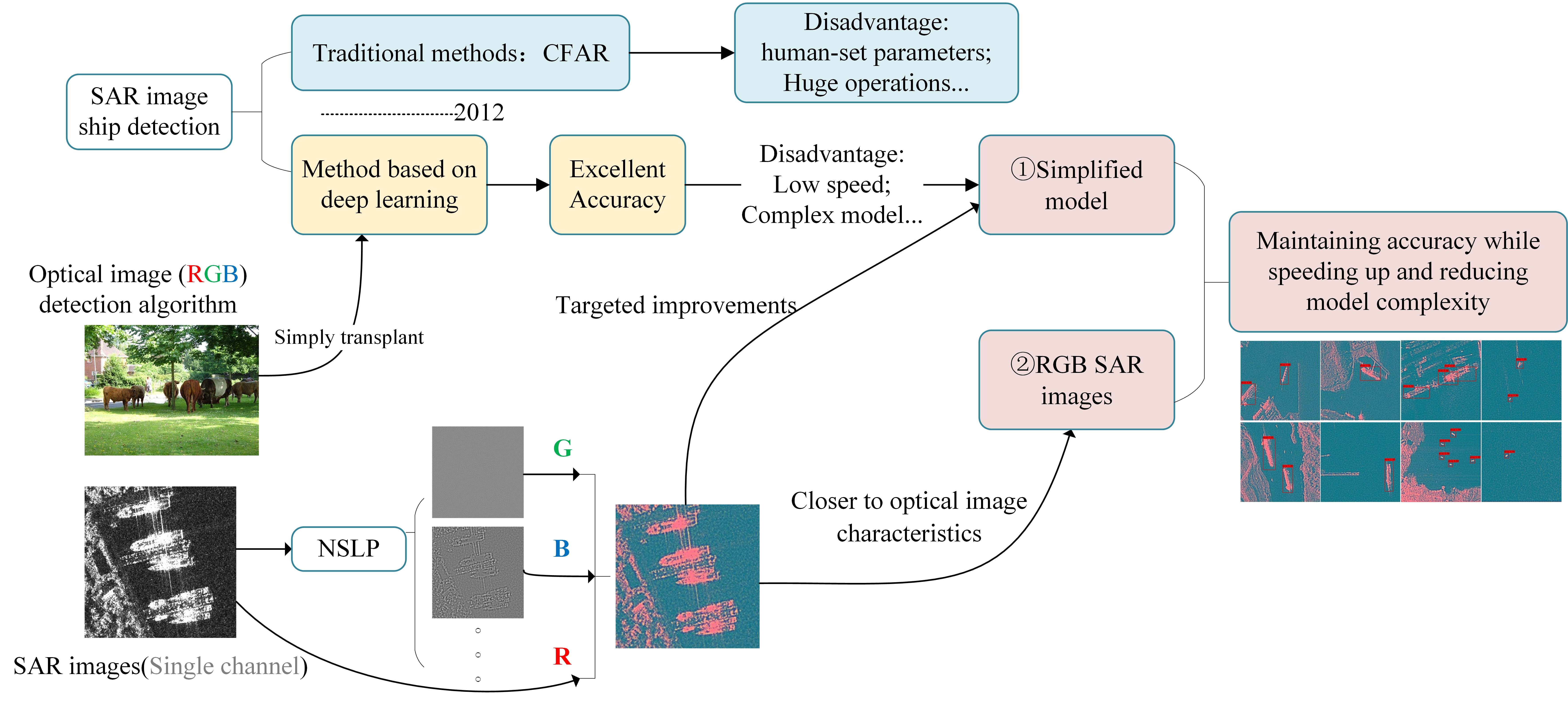
Moreover, SAR image ship detection is transposed from optical image detection, but this still has significant differences which are previously ignored by researchers. Optical images usually consist of image data acquired by visible and partial infrared band sensors, while SAR sensors operate in the microwave band. SAR images have a relatively low resolution and low signal-to-noise ratio, so the amplitude information contained in SAR images is far from the same level of imaging as optical images; Visible optical images often contain multiple bands of grey-scale information, represented by a combination of three color channels, RGB or HSV, to facilitate target recognition and classification extraction, while SAR images, on the other hand, only record the echo information of one band. Existing image detection research is more focused on RGB three-channel optical image detection and recognition, and has not been optimized for the single-channel, low resolution, and low signal-to-noise ratio characteristics of SAR images. In particular, the single-channel characteristics of SAR images make most of the current migration applications simply fill the single-channel replication with three channels, which greatly wastes the multi-channel feature extraction potential of neural networks, and how to better use the remaining two channels for SAR image processing to improve algorithm performance is also the direction of next research. On the other hand, the proportion of ships in the near-shore dock and the wide sea context is different and mostly does not exceed 10% of the whole image, so we can extract features from different perceptual fields while reducing the number of network layers to simplify the model and improve accuracy.
In this paper, we use the state-of-the-art YOLO-V4 [13], the latest version of the widely recognized YOLO algorithm, the well-known sliding window-based bounding box deep learning model in computer vision, as the basis for fast, accurate, and low-equipment-required real-time ship detection. Additionally, we introduce a new non-subsampling laplacian pyramid decomposition (NSLP) image pre-processing method for extracting contour information and denoising, expanding the single-channel SAR image information to three channels. Finally, we propose a new lightweight network YOLO-V4-light for the NSLP-processed SAR images, which significantly increases the speed of detection and significantly reduces model complexity with guaranteed accuracy. We evaluated the performance of Faster R-CNN, YOLOv4, and YOLO-V4-light was evaluated on the SSDD using a mobile RTX2060 GPU. The proposed algorithm model has lower complexity, shorter training time and detection time, and higher AP.
The main contributions of our work are as follows.
- The proposed image preprocessing method expands the single-channel SAR image originally sent to the network for learning to three channels, with ship target contour information while reducing the impact of speckle noise, making full use of network extraction capabilities, and increasing network interpretability.
- Aiming at the existing advanced and complex detection algorithms, combined with the above-mentioned preprocessing methods, a lighter network model is proposed. Compared with the existing methods, the training time is shorter, the detection speed is fast, the accuracy is high, and the hardware requirements are low.
2. Methods
2.1. YOLO-V4 Algorithm Description
In this paper, we construct an end-to-end convolutional neural network based on YOLO-V4 for ship detection. YOLO-V4 is another optimization after YOLO-V3 [14]. Based on the original YOLO target detection architecture, it adopts the best optimization strategies in the field of CNN in recent years, with different degrees of optimization in various aspects from data processing, backbone network, network training, activation function, loss function, etc.
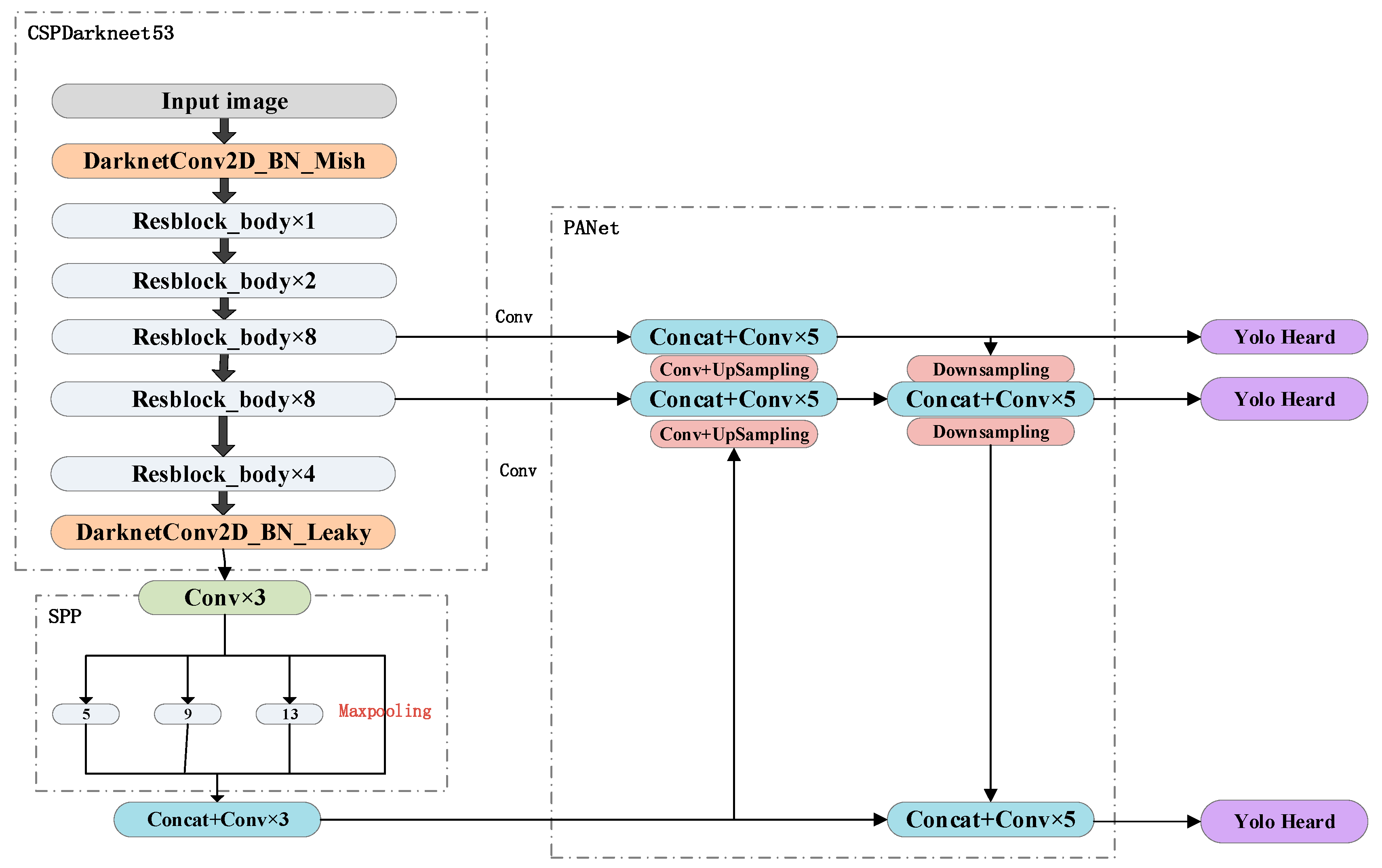
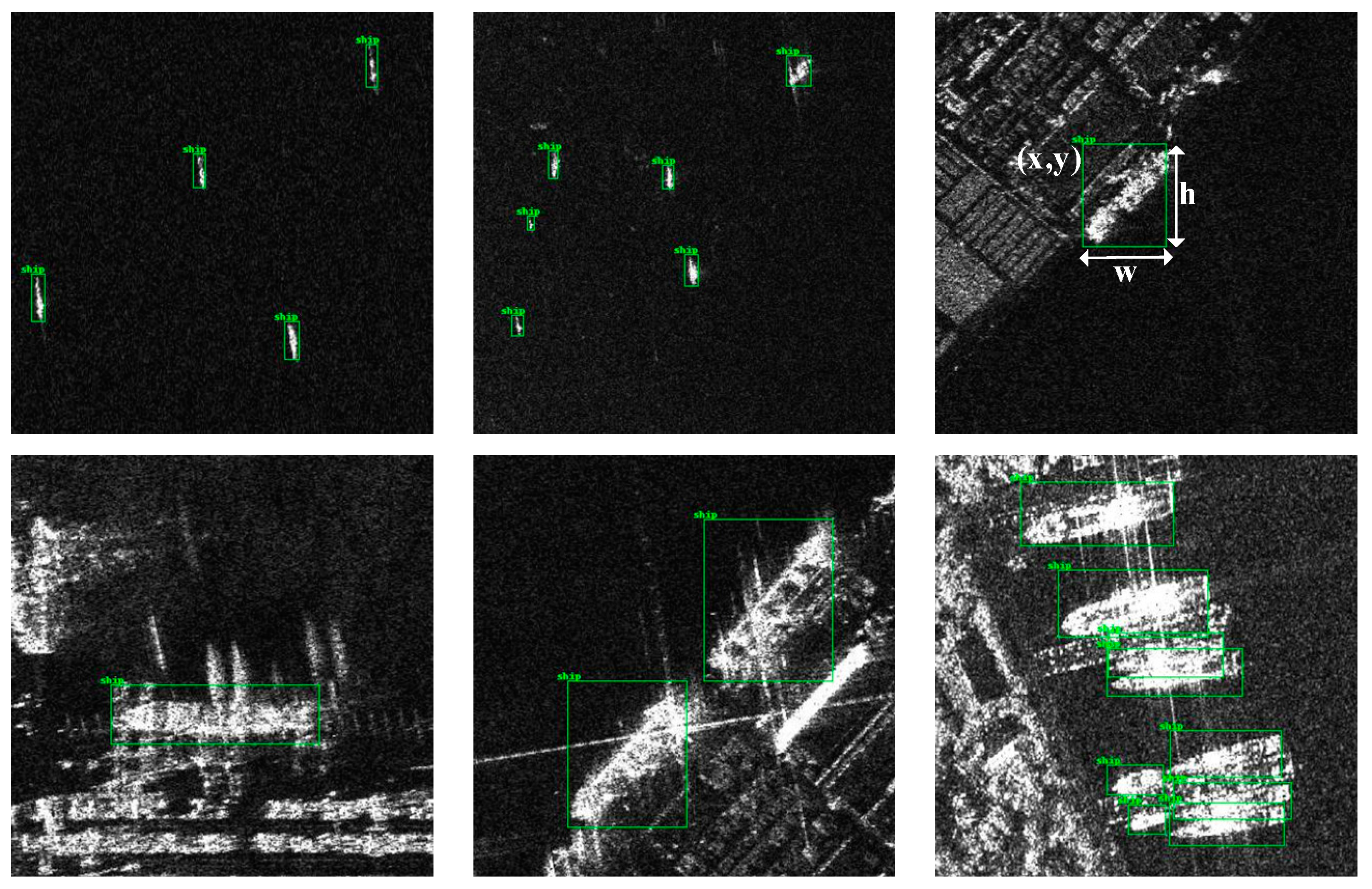
YOLO solves object detection as a regression problem, dividing the entire image into a grid, each grid being responsible for detecting objects that “fall” into that grid. If a grid happens to contain the center of an object, then this grid is responsible for detecting the object that has fallen into it. Each Bounding box contains five components:(x, y, w, h, c), the (x, y) represent the normalized center coordinates of the predicted object for that grid; (w, h) represent the normalized width and height of the Bounding box; c reflects whether the current bounding box contains an object and the accuracy of the object position, determined mainly by whether it contains a target and the IoU (Intersection over Union) of the predicted box and the ground truth. Each grid is pre-defined with three different sizes (corresponding to different perceptual fields) of a priori frames, generating a total of S × S × ((N + 5) × 3) dimensions of feature data for the final prediction, where N represents the type of object detected (1 for the SSDD, 20 for the PASCAL VOC 2007 dataset [15] and 80 for the COCO dataset [16]), and then the prediction frames are continuously scaled according to the real frames. The input image size is resized to either 416 × 416 or 608 × 608 and fed into the network for training, with the network structure shown under Figure 1 as follows.
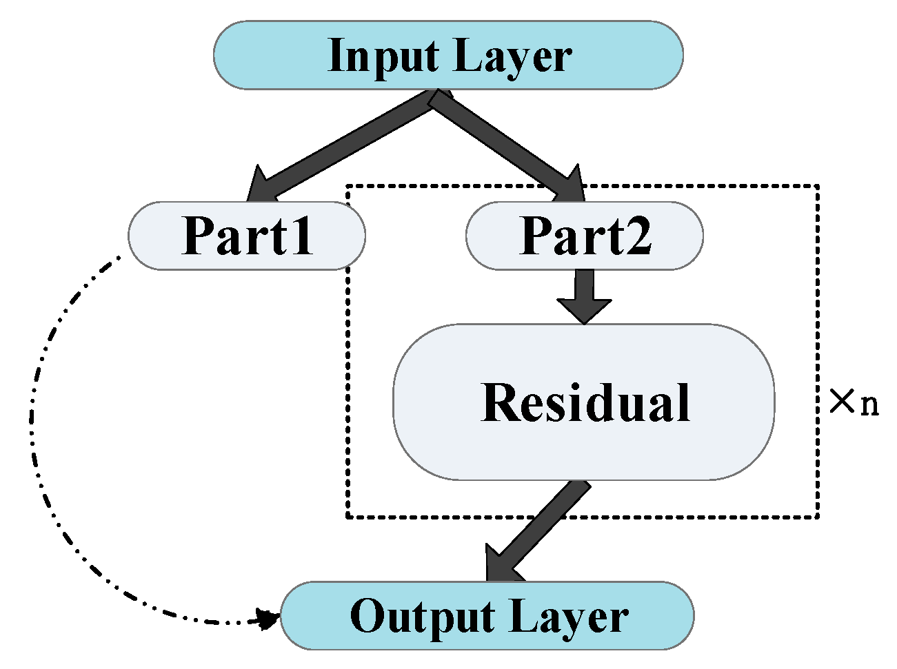
Firstly, compared to YOLO-V3, the backbone extraction network was replaced by DarkeNet-19 with CSPDarkeNet53, while retaining important features of the Residual in DarkeNet53. Residual is essentially performing a 3 × 3 convolution with a step size of 2, then saving that convolution layer, performing another 1 × 1 convolution and a 3 × 3 convolution, and adding this result to the layer as the final result. Its internal residual block uses jump connections to alleviate the problem of gradient disappearance caused by increasing depth in deep neural networks, and applies a Cross Stage Partial Network (CSP-Net) structure, Figure 2 shows its structure schematically, splitting the original stack of residual blocks into two parts: the backbone part continues the original stack of residual blocks; the other part like a residual edge, is directly connected to the end after a small amount of processing, so it can be considered that there is a large residual edge in the CSP, which is beneficial for enhancing the learning ability of CNN, eliminating computational bottlenecks and reducing memory costs [17].
Secondly, the Spatial Pyramid Pooling (SPP) structure was introduced to participate in the convolution of the last feature layer of CSPdarknet53, and then after three DarknetConv2D_BN_Leaky convolutions of the last feature layer of CSPdarknet53, finally four different scales were used for maximum pooling, with pooling kernel sizes of 13 × 13, 9 × 9, 5 × 5, and 1 × 1 (no processing), which can greatly increase the perceptual field and separate the most significant contextual features.
After the backbone network extracts the three useful feature layers and inputs them into the feature pyramid, YOLO-V4 chooses the instance segmentation algorithm Path Aggregation Network (PANet) [18] as the network for enhanced feature extraction. The most important difference that distinguishes this feature extraction network from traditional feature extraction networks is that, after completing the feature pyramid from bottom to top, top-to-bottom feature extraction is also performed. the FPN is top-down, passing down the strong semantic features from the higher levels to augment the whole pyramid, although only the semantic information is augmented and no localization information is passed on. PANet, on the other hand, addresses this by adding a bottom-up pyramid, and such an operation complements FPN by passing up the strong localization features from the lower levels. The optimized fused features will be used for target detection. After the model has finished training, the feature layer predictions are decoded, i.e.: each grid point is added with its corresponding x and y, the result of this addition is the center of the prediction frame, and then the length and width of the prediction frame are calculated using the combination of the prior frame and h and w. The final filtering is done using score sorting and non-maximal suppression, which gives the position of the whole prediction frame.
Although YOLO-V4 has an excellent performance in the field of target detection, as mentioned earlier, it is also a computationally intensive algorithm. Current surface ship computers may not be able to complete migratory training learning to cope with real-time changing conditions when faced with this type of algorithm, with problems such as too long training times, slow detection speeds, and too large models limiting the practical application of the algorithm.
2.2. Algorithm Design and Improvement
2.2.1. Construction of Three-Channel RGB SAR Image
Due to the single-channel characteristics of SAR images, most of the datasets used for research and testing are simply copied from single-channel grayscale images and then expanded to three-channel images, that is, the color values of the three RGB color channels are identical. In this section, we seek additional information useful for detection from the original SAR image to replace the same two channels and construct a completely new RGB SAR image.
The unique contour features of a ship are characteristics that are difficult to be found in various man-made clutter on the coastline. Using the ship’s contour features as a criterion for target detection and identification can effectively improve the sensitivity and accuracy of detection even in complex background conditions, and is very suitable for target detection in complex backgrounds.
This paper introduces Non-Subsampling Laplacian Pyramid Decomposition (NSLP) to address the single-channel characteristics of SAR images by using the wavelet transform principle. NSLP can extract the ship morphological features from the original image by decomposing and transforming the SAR image and construct a new channel image to highlight the ship contour information while reducing the effect of speckle noise.
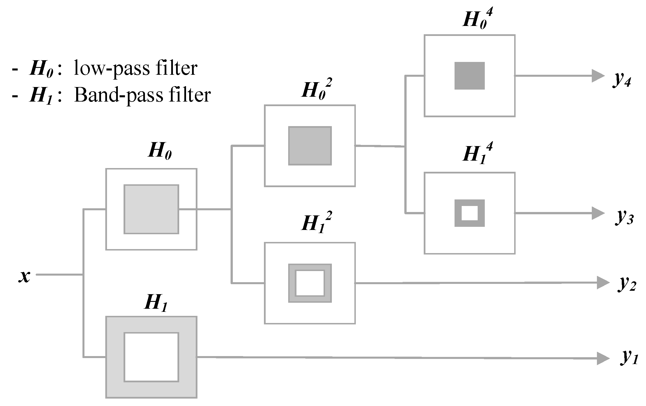
The basic principle of NSLP: NSLP is a decomposition algorithm based on the Laplacian pyramid (LP) Non-Subsampled Contourlet Transform (NSCT). Both are widely used in the field of image contour transformation [19,20]. We borrowed the idea from NSCT and added a Non-Subsampled Pyramid Filter Bank (NSPFB) to make the decomposed image translation invariant. At the same time, it has the same multi-scale feature as the LP algorithm, which can decompose images at different scales. Difference from LP decomposition, NSLP does not downsample the components after filtering but upsamples the filter accordingly. That is to say, the secondary filter of the NSLP can be obtained by upsampling the filter of the previous stage with a step size of 2. When an image undergoes the L-level NSLP decomposition, L + 1 subband images with the same size as the original image can be obtained.
Figure 3 shows the NSLP structure of a three-stage filter cascade, where, for example, the low-pass filter is represented H0; is the second-stage filter obtained by upsampling the previous filter in steps of two; the other filters in the figure follow the same pattern. Let the i-th image feature be mapped as and the L + 1 subbands will be obtained by L-layer NSLP decomposition as follows.
where L is the number of NSLP filter levels and (m, n) denotes the pixel position in the picture, the m-th row and nth column of the pixel matrix. The decomposed subbands are denoted as , where at the output of each filter level is the high-frequency component obtained from each level of decomposition, and at the output of the last filter level is the low-frequency component.
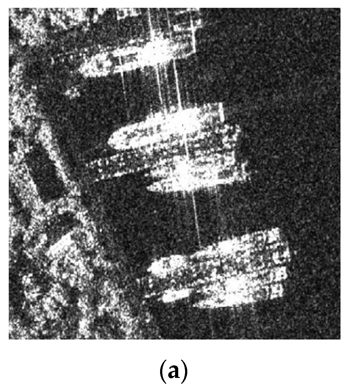
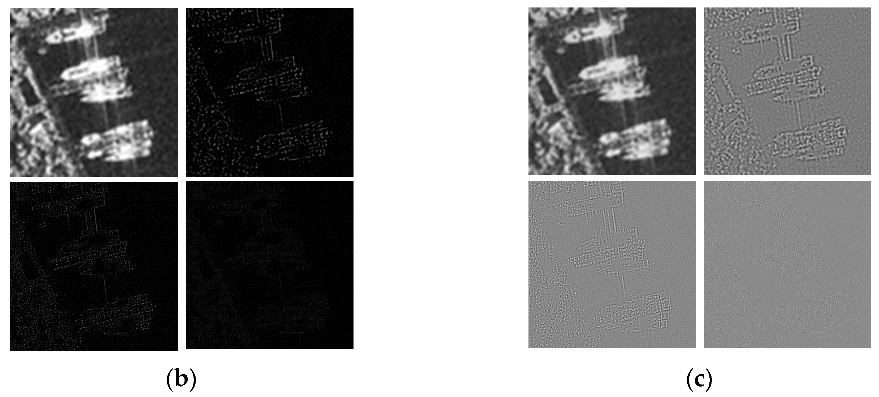
We take a SAR image in the SSDD as an example, and Figure 4a shows the original image, where the shoreline of the quay and the ships in the near harbor are linked together and are both highlighted. Figure 4b shows the four subbands after NSLP decomposition, corresponding to {y4 y3 y2 y1} in Figure 3, where the first subgraph corresponds to {y4}, which has undergone three decompositions in the NSLP structure, and the low-frequency subbands obtained from each layer of decomposition will continue to be decomposed in the next layer, and the scale of the filter is twice that of the previous layer of decomposition, and the final obtained also {y4} has the largest decomposition scale. It contains most of the information of the ship, the pier, and the coast in the original image, and the overall area information is relatively complete. The multiple low-frequency filtering makes the intensity of the scattering noise significantly reduced, but the absence of the high-frequency component makes the image clarity decrease significantly, and the boundaries of the targets in the image are more difficult to distinguish. The remaining three sub-maps correspond to {y3 y2 y1} which are high-frequency subbands obtained from different scale decompositions. Although they contain less visible information than the low-frequency self-bands, they extract the important contour information of the original image and evenly disperse the scattering noise into the three sub-bands. The high-frequency subbands can reflect the contour information of the ship SAR image well, and as the scattering noise is non-uniformly distributed in multiple subbands, the high-frequency subbands only contain part of the attenuated scattering noise, which effectively reduces the effect of scattering noise when composing the three-channel image. We then normalized the four subbands of the decomposed image to obtain the four normalized subbands shown in Figure 4c.
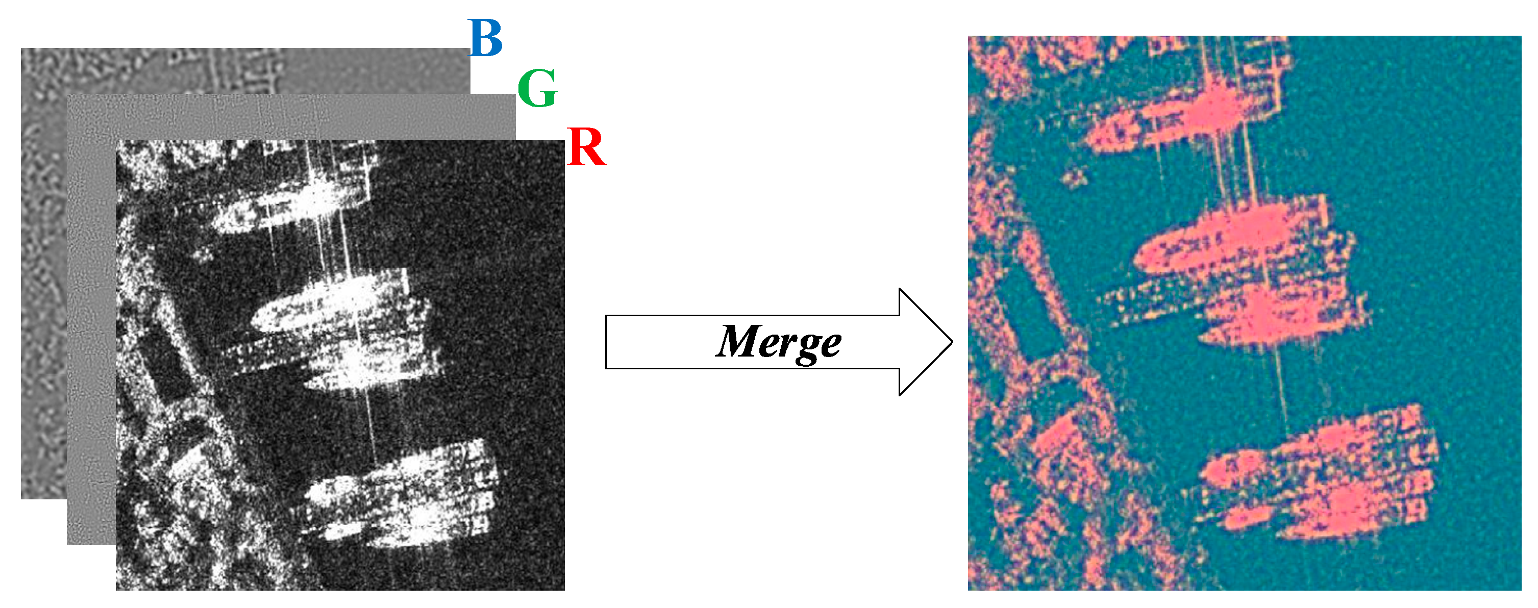
After the above operation, we transform the single-channel polarization feature decomposition into three contour subbands and one low-frequency subband., and then we select the original image and the two normalized high-frequency subbands that contain the ship’s contour information, respectively, as the combination of the three color channels of R, G, B of the new image to form a three-channel polarized SAR image. as shown in Figure 5. This method retains all the information in the original image and adds important contour information, while reducing the effect of scattering noise compared to the case where all three channels are original images, greatly enriching the information contained in the training data. The new images can guide the network in feature mining and selection in the low-frequency subbands and contour subbands, which can be mapped into the CNN to improve model training efficiency, balance the feature contribution of each subband, reduce noise interference and enhance the sensitivity and accuracy of model detection.
We performed the above operation on the SSDD to generate a completely new three-channel dataset, RGB-SSDD, with the same divisions.
2.2.2. Light-Weighting Model
When we consider the limitations of the application scenario, the goodness of the predictive model is not the only factor to consider, you also need to worry about:
- (1).
- the amount of space the model takes up in equipment—a single model of Faster R-CNN may add Hundreds of MBs to the download size of equipment
- (2).
- the amount of memory used at runtime—when the model runs out of free memory algorithm may be terminated by the system
- (3).
- how fast the model runs—especially in emergency situations where real-time is essential [21].
The vast majority of authors of academic papers never worry about these things, they train and run the designed models on huge desktop GPU computing clusters. However, the light-weighting of the model can reduce the need to communicate with the server; using fewer parameters is more suitable for deployment on embedded, mobile devices such as FPGA where memory is first available, and also for faster downloading and deployment from the cloud servers. The ship detection algorithm should be developed toward a better balance of accuracy, speed, and lightness to speed up the process of serving the safety of the territorial sea.
The field of deep learning typically measures the complexity of an algorithm model using floating-point operations (FLOPs) (s denotes plural numbers), which can be interpreted as computational effort. Assuming a sliding window implementation of convolution and ignoring the non-linear computational overhead, the FLOP of the convolution kernel is:
where , is the height, width, and the number of channels with the input element map (the input image). is the core width, is the number of output channels, and for fully connected layer networks is , where is the input size and is the output size. Similar to it is the MADD (Multiply-Add) [22].
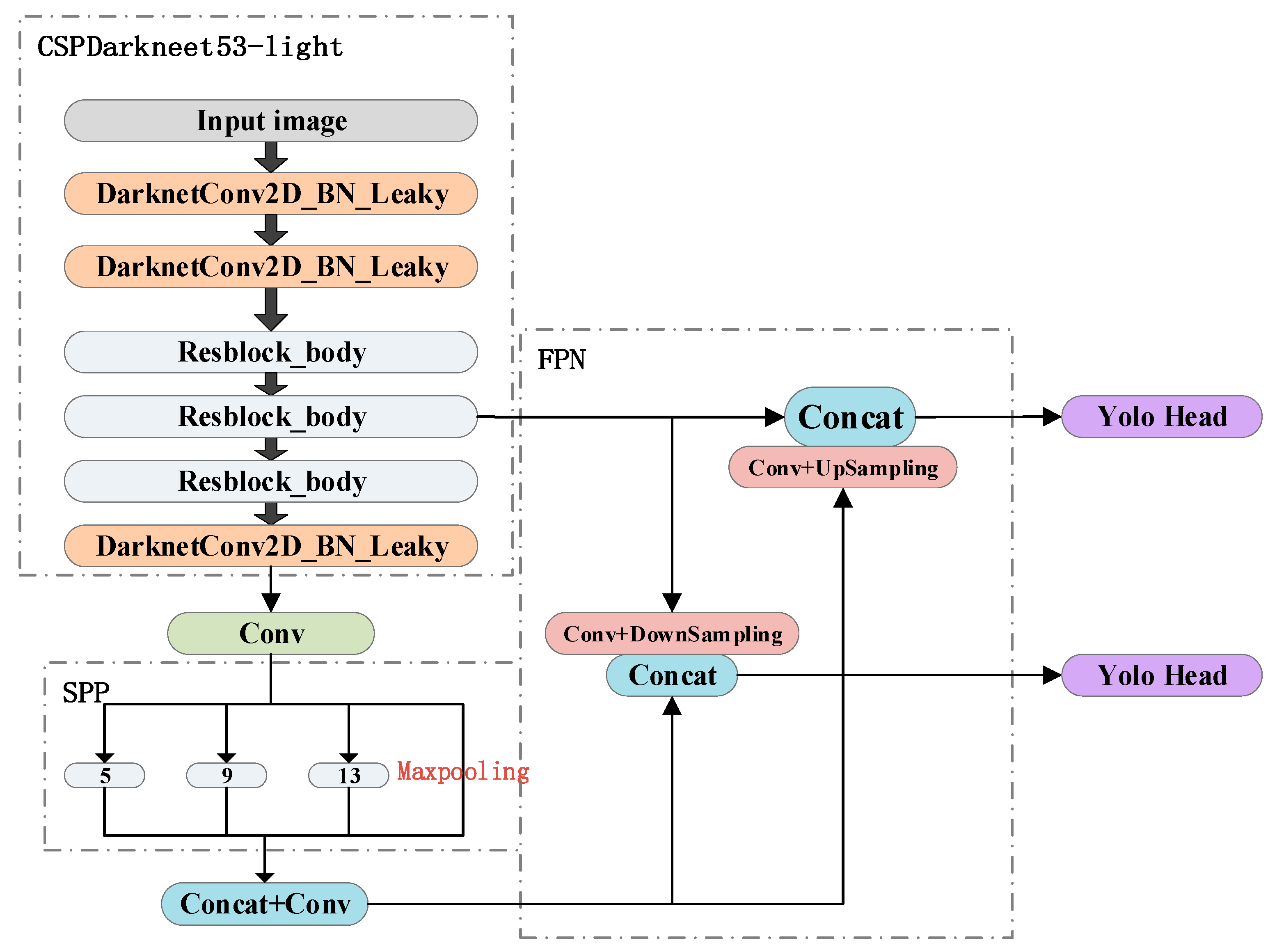
This paper borrows ideas from the GitHub open source project [23] and combines the new three-channel SAR dataset that contains denoising and contouring information to propose YOLO-V4-light, which decreases from 60 million parameters in YOLO-V4 to 6 million, resulting in a significant reduction in model size and hardware computing power requirements, and a significant increase in training speed and prediction speed. The network structure is shown in Figure 6. Comparing Figure 6 and Figure 1, the new light network has greatly reduced the number of convolutional layers in CSPDarkNet53, kept the SPP structure to facilitate the extraction of contour features of ships of different sizes. Drawing on PANet’s idea of iterative feature extraction, the new fused features are obtained by up-sampling the deep features and fusing them with the shallow features, and down-sampling the shallow features and fusing them with the deep features for the final discriminant detection. This bottom-up information fusion is more conducive to the precise positioning of ship detection. Iterative extraction and fusion of features facilitate the better use of the feature information contained in the new three-channel SAR image.
Table 1 shows a comparison of the parameter sizes of several algorithmic networks. The parameters of the Light algorithm model mentioned in this paper are only 1/20 of Faster R-CNN and 1/10 of YOLO-V4; the number of floating-point operations is only 3.2% and 11.8% of the two; the demand of read–write memory at runtime is only 0.05% and 15% of the two. Another [24] shows that the parameter scale of Faster-RCNN is already much smaller than YOLO V1-V3, RetinaNet, and comparable to SSD. In summary, the proposed new network has a definite advantage in terms of model parameter size and running memory.
3. Experimental and Results
3.1. Dataset
As the nature of deep learning dictates that only a dataset with a sufficiently large amount of data and significant accompanying target features can be selected to show a clear advantage over other traditional methods, we use the SSDD of ships in packet-swapped different environmental contexts [25], which was mainly acquired by RadarSat-2, TerraSAR-X and Sentinel-1 sensors in four polarizations, HH, HV, VV, and VH, in Yantai, China, and Visakhapatnam, India, with a resolution of 1–15 m, and ship target scenarios including open ocean and offshore ports. A total of 1160 images of size 416 × 416, containing a total of 2456 ships, with an average of 2.12 ships per image. We use LabelImg software to annotate all the images and convert the annotation information into a standard XML format, with each target’s box represented as (x, y, w, h), as shown in Figure 7. This dataset is a typical dataset used by researchers in the field of SAR image detection to evaluate the performance of their algorithms.
We generate a new three-channel dataset RGB-SDDD for the SSDD according to the method proposed in Section 2.2.1 and divide the two datasets into a train set, a test set, and a validation set in the same ratio of 7:2:1, each containing a wide sea area, an inshore dock and different ships of different sizes, as shown in Table 2.
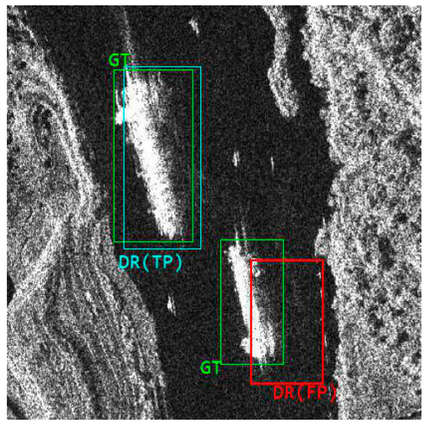
Average Precision (AP) is the most common metric used to evaluate all types of models and involves Precision, Recall, and Intersection over Union (IoU). True positive (TP) is an instance where the model classification considers a positive sample and is indeed a positive sample, false negative (FP) is an instance where the classifier considers a positive sample but is not a positive sample, and FN is an instance where the classifier considers a negative sample but is not a negative sample. instances. IoU is calculated as the ratio of the overlap between the prediction frame and the real frame:
where is the area of the intersection of the prediction frame and the ground truth, and is the area of the concurrent set of the two. When the IoU is greater than 0.5, which means that the prediction frame and the real frame have at least half overlap, then the ship detection is considered correct, i.e., TP, otherwise the ship detection is considered incorrect, i.e., FN, and the relationship is as in Figure 8.
The AP and F1metrics relate to Precision and Recall and are calculated as follows:
The AP value, on the other hand, is the area enclosed under the Precision and Recall curves, effectively avoiding the high level of false detections and missed detections that may occur with a single evaluation criterion, with higher AP indicating better detection performance of the model.
3.2. Experiment 1
We trained the YOLO-V4-based ship detection model on SSDD while introducing YOLO-V4-tiny [23], a simplified version of YOLO-V4, as a comparison. All experiments were performed on a portable computer with AMD Ryzen 7-4800H at 2.9 GHz, 8 cores and 16 threads, 8G × 2 RAM, NVIDIA GeForce RTX 2060, CUDA 10.0 cuDNN7.6.5, and Windows 10 as the operating system. Experiments were conducted to compare and evaluate various ship detection algorithms in terms of accuracy, speed, and low hardware requirements. The results validate the effectiveness and correctness of the image processing approach and the lightweight network modification.
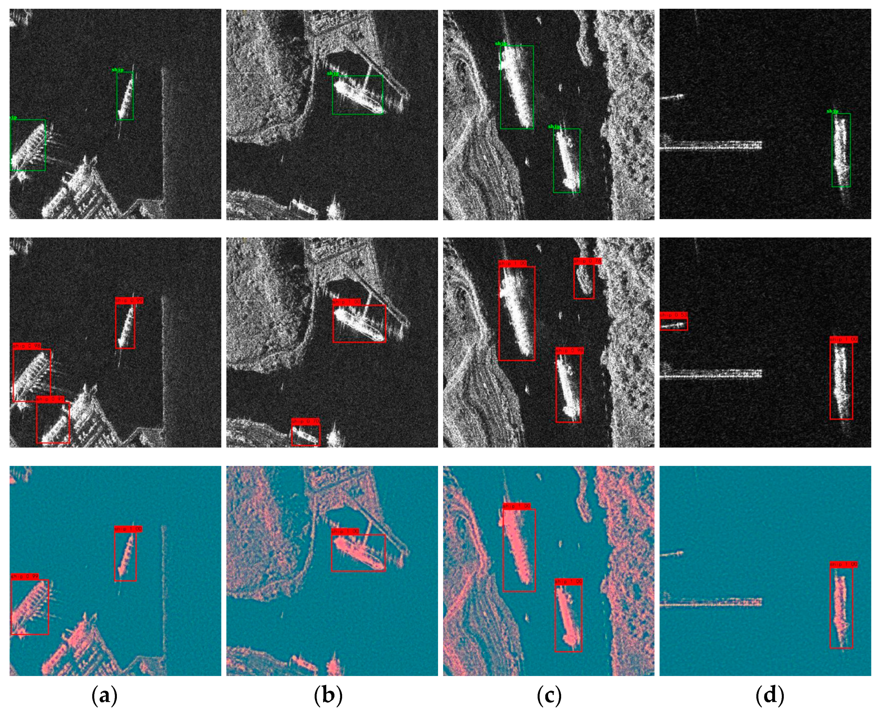
Figure 9 shows some of the results of the YOLO-V4 in the test set, with eight different scenarios, resolutions, and ship sizes selected to demonstrate its detection performance. We can see that YOLO-V4 shows good detection capability for images of ships docked at near-shore piers, ships sailing in wide-open waters and near-shore bays and rivers, as well as images of ships with degraded image quality due to noise.
All the above results are the average results of the parameter settings under the mobile hardware configuration, we can see that YOLO-V4 has a relatively large performance improvement in both accuracy and time compared to Faster-R-CNN. However, for the actual application environment of maritime ship detection, it still does not satisfy the lightweight of the algorithm model and the real-time speed of detection, especially in the process of algorithm training, the minimum GPU computing power requirement is NVIDIA GTX-1080ti or GTX-2080 GPU. This volume of GPU is an almost impossible hardware configuration for both the frontline battlefield and coastal policing.
Table 1, Table 3 and Table 4 show the evaluation indexes of YOLO-V4 under the SSDD, it can be seen that: compared with FasterR-CNN, YOLO-V4 has great advantages in all aspects except for the larger model file. Especially in terms of accuracy, Faster R-CNN sacrifices speed for accuracy advantage in SAR ship detection is not effective. Despite having an excellent recall rate, the excessive false detection rate creates an imbalance between accuracy and recall. This imbalance is highly undesirable in ship detection. The lightweight tiny network, although with a reduced AP due to the very reduced network depth, still balances accuracy and recall well and achieves good detection performance, still needs to be optimized to meet the hard AP requirements.
3.3. Experiment 2
Experiment 1 shows that YOLO-V4 is not well suited to the needs of high-speed lightweight. We continue to try to explore the performance of the new image processing method NSLP and the new high-speed lightweight model YOLO-V4-light for ship detection. Experiments were conducted using the new network architecture proposed in Section 2.2.2 in comparison with the tiny algorithm, loaded with pre-trained models pre-trained with the VOC dataset (experiments show that the VOC pre-trained model with 20 classes performs better than the COCO dataset with 80 classes for single-class ship detection). Since the pre-trained weight backbone network is backward compatible with the ship detection backbone network, we chose to freeze the training in the first 50 epochs and choose a higher initial learning rate of 0.001 to focus more resources on training the later part of the network parameters, which resulted in a significant improvement in both time and resource utilization. This results in a significant improvement in both time and resource utilization. The latter 150 epochs of unfrozen training, setting a lower initial learning rate of 0.0001 and fine-tuning the network using a simulated annealing strategy, were trained and tested under both SSDD and RGB-SSDD, and the results validated the effectiveness and correctness of the image processing approach and the lightweight network modification with metrics such as accuracy, speed, and small hardware requirements.
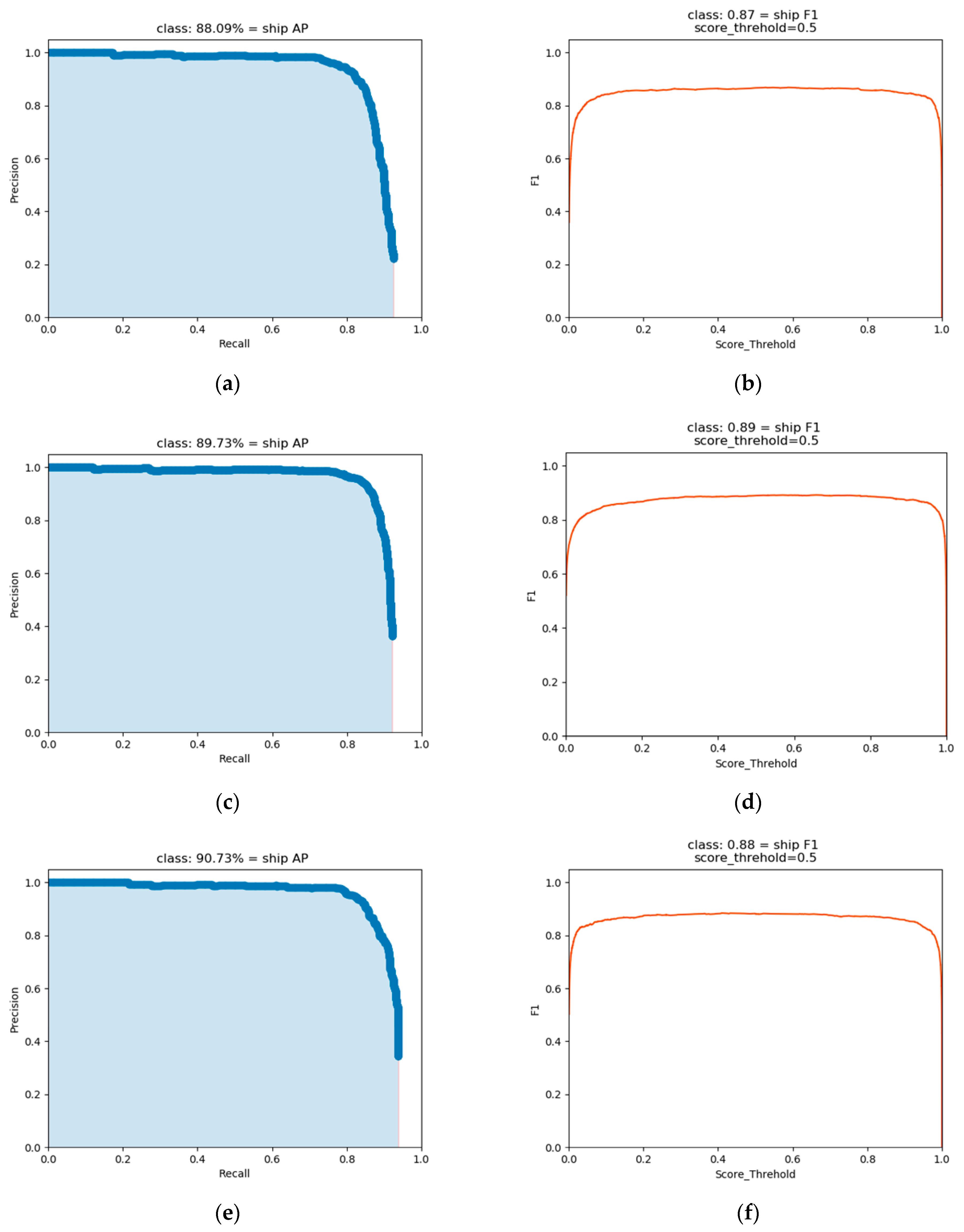
Table 1 shows the differences in the overall parameters, memory occupied, and the number of operations; Table 5 shows the performance of ship detection under various types of lightweight networks and different datasets, the results of the table are the average test results of multiple models. Figure 10 shows the performance metrics of AP, F1 for some experiments, where (a,b), (c,d), and (e,f) correspond to rows 1–3 of Table 5, respectively. The experimental results demonstrate that YOLO-V4-tiny guarantees accuracy while
- (1).
- Significant reduction in training time (12% for Faster R-CNN, 25% for YOLO-V4)
- (2).
- Significant reduction in model size (21% for Faster R-CNN, 9.2% for YOLO-V4)
- (3).
- Significant reduction in single-frame detection time (9.7% for Faster R-CNN, 27.7% for YOLO-V4)
The effectiveness of the three-channel contour image synthesis method proposed in Section 2.2 was also verified: 1.56% improvement in AP. The new model YOLO-V4-light, proposed for the three-channel data processing method, improves AP by 2.29%, reaches 90.37%, without much change in model size, training time, and detection time, and outperforms the AP of YOLO-V2-reduced and G-CNN in the literature [11,12] by 89.76% and 90.16%. subject to the lack of GPU the method cannot be fully reproduced and compared due to the lack of GPUs, but the GPU computing power required for YOLO-V4-light (mobile RTX 2060) is much less than the two experiments in the literature (GTX 1080 and TITAN X). The validity of the adaptation to the three-channel data network structure proposed in Section 2.2.2 is verified.
4. Result
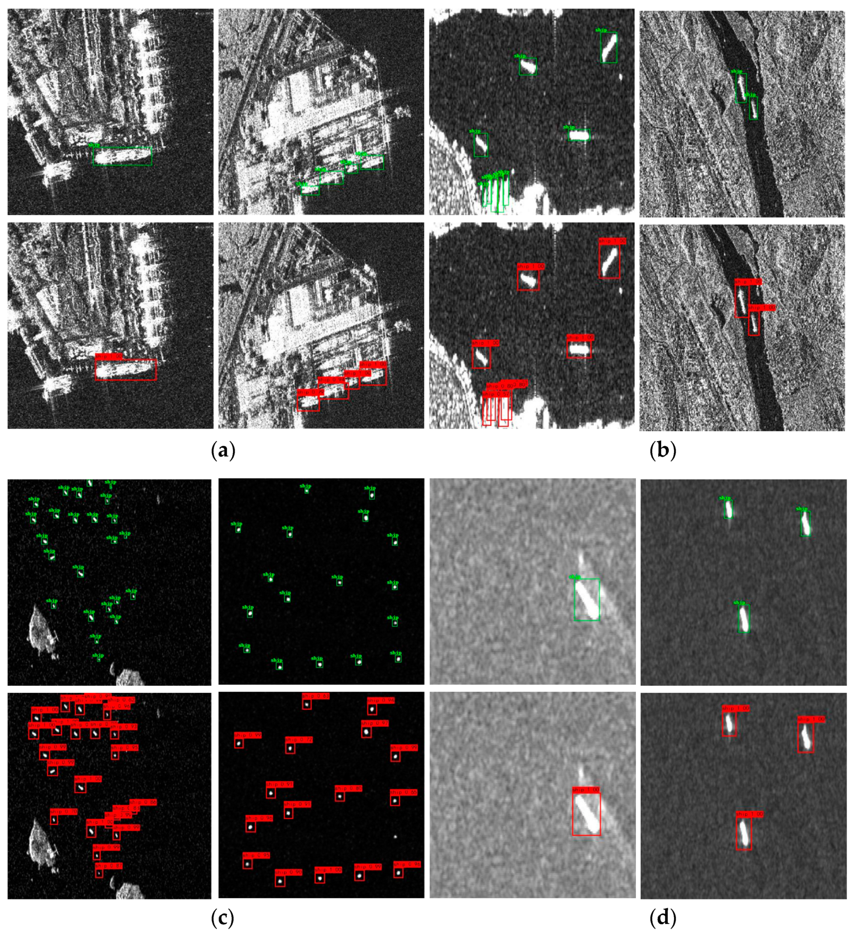
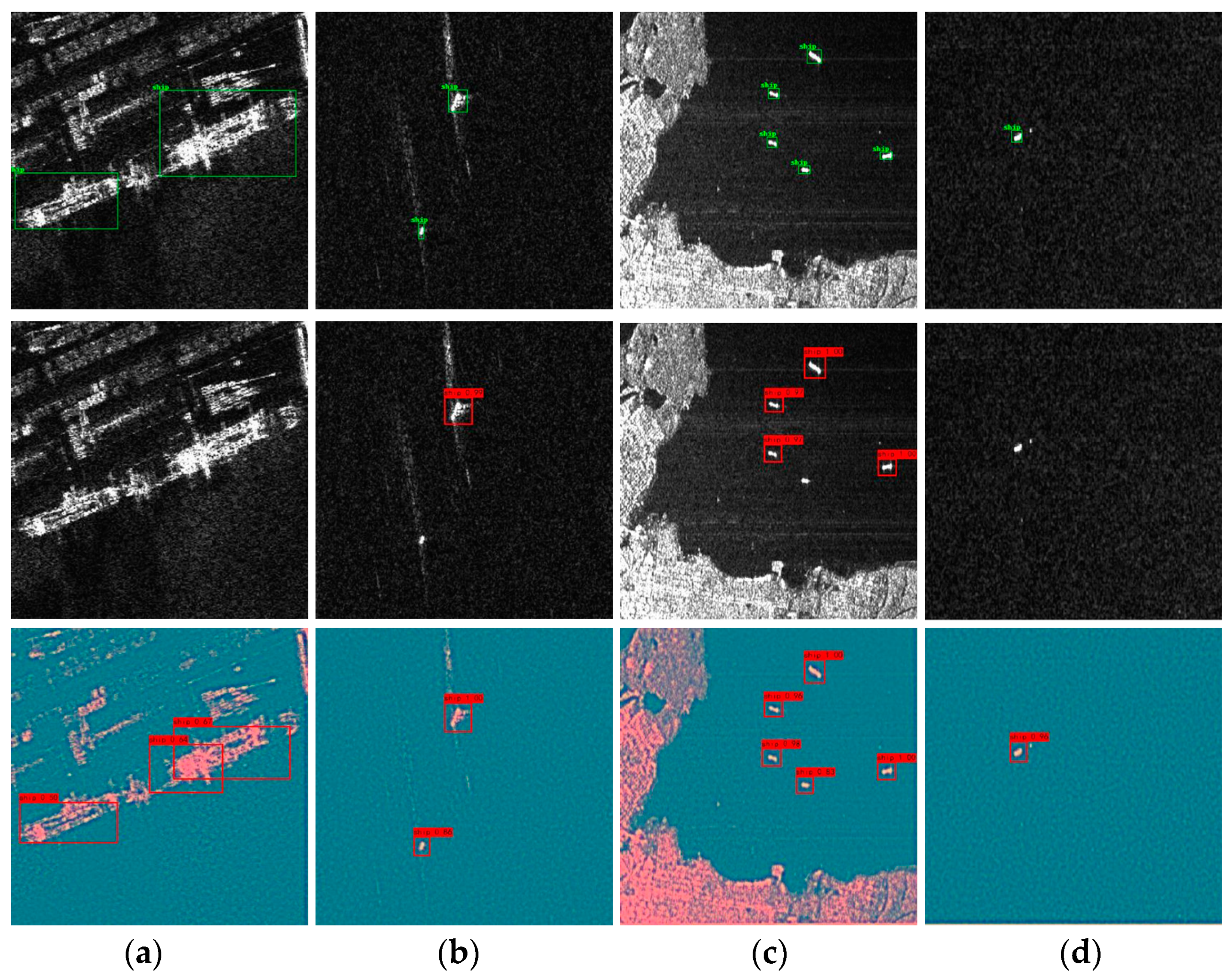
For the same lightweight algorithm, on the one hand, the tiny algorithm without the three-channel dataset is weak in recognizing the ship’s contour, and in Figure 11a,b the shore jetty embankment is mistakenly detected as a ship, and (c) (d) the channel shoal and jetty trestle are mistakenly detected as a ship. The light algorithm with the new three-channel dataset can avoid the occurrence of false identification and accurately distinguish ships from similar embankments and shoals. On the other hand, the new proposed light algorithm in this paper, with the addition of SPP structure and multiple fused feature pyramid network, can also detect large ships near shore in Figure 12a and small target ships in (b–d) over a wide sea surface more accurately. The false detection rate is effectively reduced, which also confirms the improvement of AP indicators in Figure 10a,c,e. The above analysis verifies the correctness and feasibility of the proposed ship detection algorithm in terms of both experimental performance metrics and actual detection results.
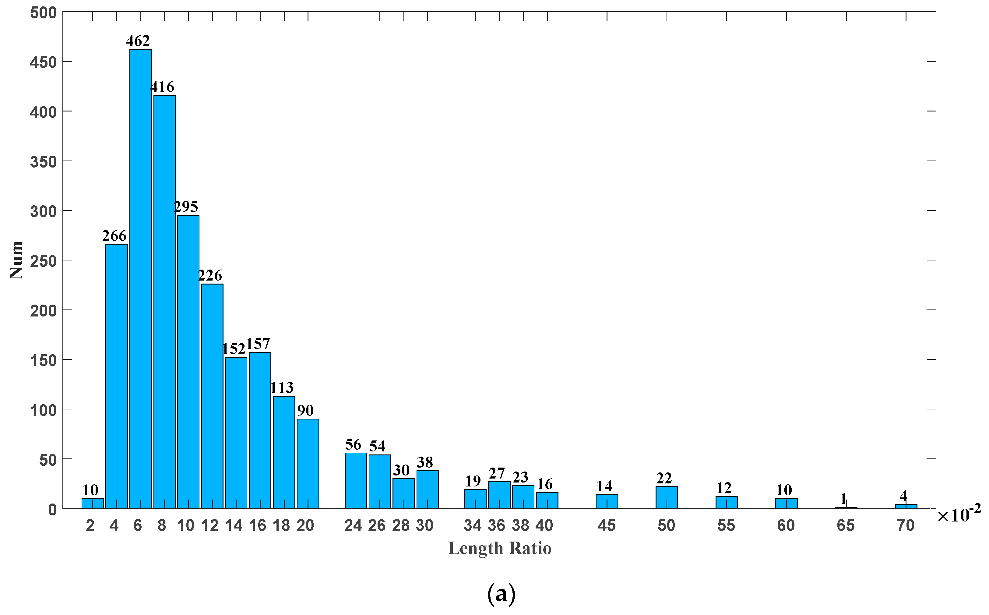
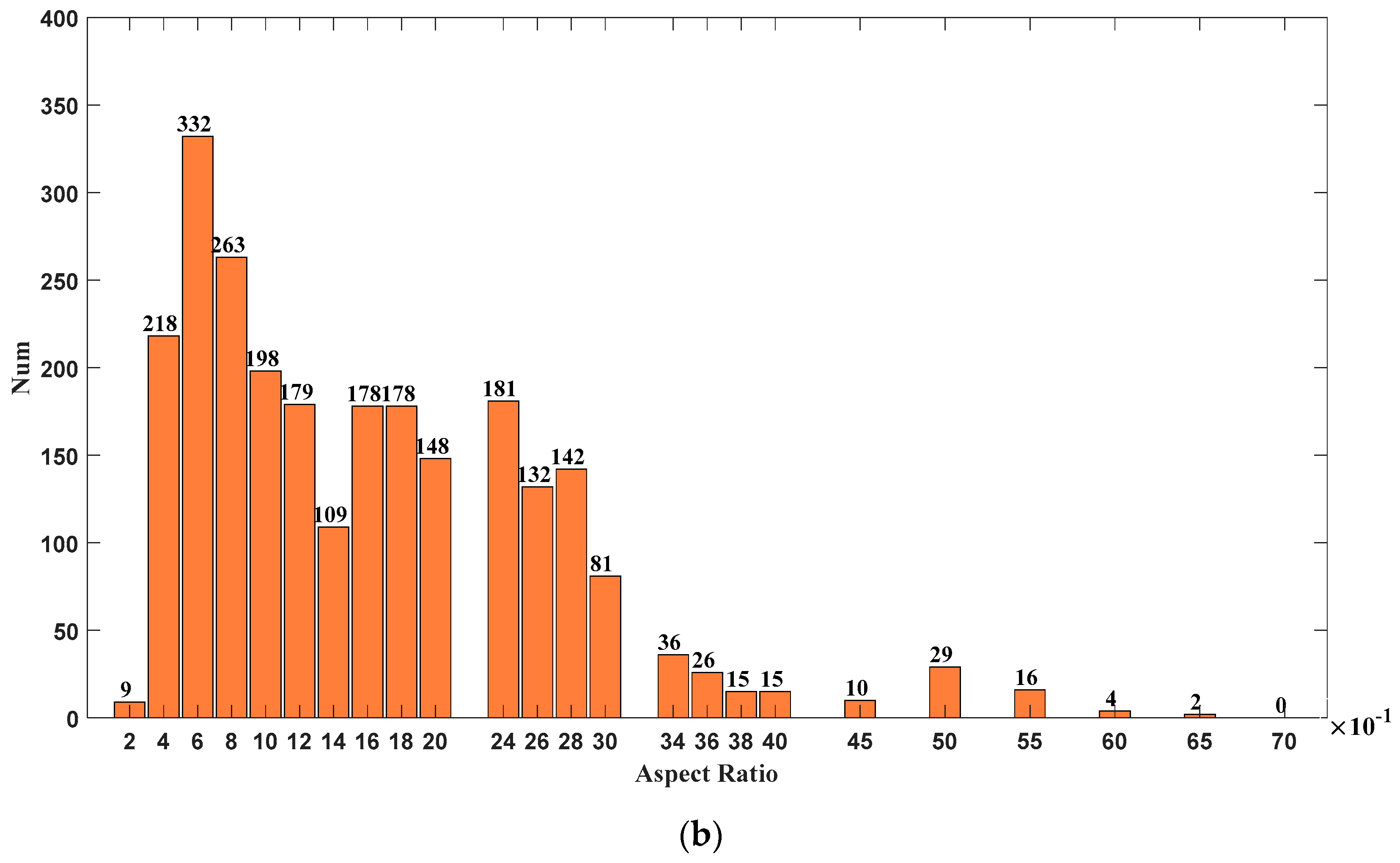
From the perspective of the application target, the deep learning target detection algorithm mainly targets the images of life scenes contained in the VOC and COCO datasets, which are quite different from the SSDD. The aspect ratio of VOC is mostly 1, with a small number of 2 and 3, while ship targets are larger in length and width. It can be seen from Figure 13a that the ratio of the ship target’s length to the image size is in the range of 0.04 to 0.24, which is much smaller than the VOC’s 0.2 to 0.9. Figure 13b shows the statistical results of the aspect ratio of the ship bounding box in the SSDD. The NSLP three-channel synthesis method focuses more on the extraction of horizontal and vertical contour features and discards the bandpass directional subband feature, which is of little use for small targets. The wider distribution of aspect ratios and the more regular ship targets also contribute to the improved performance with the addition of contour information and feature pyramids.
5. Conclusions
In this paper, we first evaluate the performance of the latest YOLO-V4 deep neural network architecture for ship detection in several different scenarios. Experiments were conducted on a widely recognized dataset, and its accuracy and speed for both small vessel targets in vast seas and complex vessel targets in near-shore ports outperformed existing algorithms, and was particularly accurate in complex scenarios to a much higher degree than Faster R-CNN, although we still believe that the detection speed, model size, training time and hardware requirements of YOLO-V4 are not sufficient for current frontline safety precautions at sea. Therefore, we propose a three-channel image construction scheme based on NSLP contour extraction, which enriches the contour information of the dataset while reducing the impact of noise, and better transposes the algorithms in the field of optical image detection. At last, we combined the three-channel images with the proposed lightweight network, using only 10.3% of the YOLO-V4 algorithm’s parameters and 15.8% of the memory requirement to achieve 93.8% of its AP performance, reaches 90.37%, while increasing the speed to its 3.3 times. Compared with lightweight algorithms shown in existing research, it also has an advantage in accuracy. The proposed three-channel construction method and lightweight model were verified in experiments to better meet the requirements of the actual real-time maritime ship inspection system.
Future work should aim to find more useful information about ships to enrich the redundant color channels of SAR images, and further optimize the network structure, especially for the detection performance of small and dense ships.
Author Contributions
Conceptualization, X.F.; Investigation, X.W. and Z.M.; Methodology, J.J. and R.Q.; Resources, X.F.; Validation, J.J.; Writing—original draft, J.J.; Writing—review & editing, J.J. All authors have read and agreed to the published version of the manuscript.
Funding
This research received no external funding.
Conflicts of Interest
The authors declare no conflict of interest.
References
- Leng, X.; Ji, K.; Yang, K.; Zou, H. A Bilateral CFAR Algorithm for Ship Detection in SAR Images. IEEE Geosci. Remote Sens. Lett. 2015, 12, 1536–1540. [Google Scholar] [CrossRef]
- Liao, M.; Wang, C.; Wang, Y.; Jiang, L. Using SAR Images to Detect Ships from Sea Clutter. IEEE Geosci. Remote Sens. Lett. 2008, 5, 194–198. [Google Scholar] [CrossRef]
- Krizhevsky, A.; Sutskever, I.; Hinton, G. Imagenet classification with deep convolutional neural networks. In Advances in Neural Information Processing Systems; ACM: New York, NY, USA, 2012; pp. 1097–1105. [Google Scholar]
- Girshick, R.; Donahue, J.; Darrell, T.; Malik, J. Rich Feature Hierarchies for Accurate Object Detection and Semantic Segmentation. In Proceedings of the 2014 IEEE Conference on Computer Vision and Pattern Recognition (CVPR), Columbus, OH, USA, 23–28 June 2014; pp. 580–587. [Google Scholar]
- Girshick, R. Fast R-CNN. In Proceedings of the 2015 IEEE International Conference on Computer Vision (ICCV), Santiago, Chile, 13–16 December 2015; pp. 1440–1448. [Google Scholar]
- Ren, S.; He, K.; Girshick, R.; Sun, J. Faster R-CNN: Towards Real-Time Object Detection with Region Proposal Networks. In Advances in Neural Information Processing Systems; IEEE: New York, NY, USA, 2015; pp. 91–99. [Google Scholar]
- Redmon, J.; Divvala, S.; Girshick, R.; Farhadi, A. You Only Look Once: Unified, Real-Time Object Detection. In Proceedings of the 2016 IEEE Conference on Computer Vision and Pattern Recognition (CVPR), Las Vegas, NV, USA, 27–30 June 2016; pp. 779–788. [Google Scholar]
- Liu, W.; Anguelov, D.; Erhan, D.; Szegedy, C.; Reed, S.E.; Fu, C.-Y.; Berg, A.C. SSD: Single Shot MultiBox Detector. In Proceedings of the European Conference on Computer Vision (ECCV), Amsterdam, The Netherlands, 8–16 October 2016; pp. 21–37. [Google Scholar]
- Chen, Z.; Gao, X. An Improved Algorithm for Ship Target Detection in SAR Images Based on Faster R-CNN. In Proceedings of the 2018 Ninth International Conference on Intelligent Control and Information Processing (ICICIP), Wanzhou, China, 9–11 November 2018; pp. 39–43. [Google Scholar] [CrossRef]
- Wang, R.; Xu, F.; Pei, J.; Wang, C.; Huang, Y.; Yang, J.; Wu, J. An Improved Faster R-CNN Based on MSER Decision Criterion for SAR Image Ship Detection in Harbor. In Proceedings of the IGARSS 2019—2019 IEEE International Geoscience and Remote Sensing Symposium, Yokohama, Japan, 28 July–2 August 2019; pp. 1322–1325. [Google Scholar] [CrossRef]
- Zhang, T.; Zhang, X. High-Speed Ship Detection in SAR Images Based on a Grid Convolutional Neural Network. Remote Sens. 2019, 11, 1206. [Google Scholar] [CrossRef] [Green Version]
- Chang, Y.-L.; Anagaw, A.; Chang, L.; Wang, Y.C.; Hsiao, C.-Y.; Lee, W.-H. Ship Detection Based on YOLOv2 for SAR Imagery. Remote Sens. 2019, 11, 786. [Google Scholar] [CrossRef] [Green Version]
- Bochkovskiy, A.; Wang, C.; Liao, H.M. YOLOv4: Optimal Speed and Accuracy of Object Detection. arXiv 2020, arXiv:2004.10934. Available online: https://arxiv.org/abs/2004.10934 (accessed on 12 May 2021).
- Redmon, J.; Farhadi, A. YOLOv3: An incremental improvement. arXiv 2018, arXiv:1804.02767. Available online: https://arxiv.org/abs/1804.02767 (accessed on 12 May 2021).
- Everingham, M.; van Gool, L.; Williams, C.K.; Winn, J.; Zisserman, A. The Pascal Visual Object Classes (VOC) Challenge. Int. J. Comput. Vis. 2010, 88, 303–338. [Google Scholar] [CrossRef] [Green Version]
- Lin, T.Y.; Maire, M.; Belongie, S.; Bourdev, L.; Girshick, R.; Hays, J.; Petrona, P.; Ramanan, D.; Zitnick, C.L.; Dollar, P. Microsoft COCO: Common Objects in Context. In Computer Vision ECCV 2014. ECCV 2014; Lecture Notes in Computer Science; Fleet, D., Pajdla, T., Schiele, B., Tuytelaars, T., Eds.; Springer: Cham, Switzerland, 2014; Volume 8693. [Google Scholar]
- Wang, C.-Y.; Liao, H.-Y.M.; Wu, Y.-H.; Chen, P.-Y.; Hsieh, Y.-W.; Yeh, I.-H. CSPNet: A New Backbone that can Enhance Learning Capability of CNN. In Proceedings of the IEEE/CVF Conference on Computer Vision and Pattern Recognition (CVPR) Workshops, Seattle, WA, USA, 14–19 June 2020; pp. 390–391. [Google Scholar]
- Liu, S.; Qi, L.; Qin, H.; Shi, J.; Jia, J. Path Aggregation Network for Instance Segmentation. In Proceedings of the IEEE Conference on Computer Vision and Pattern Recognition (CVPR), Salt Lake City, UT, USA, 18–23 June 2018; pp. 8759–8768. [Google Scholar]
- Qin, R.; Fu, X.; Lang, P. PolSAR Image Classification Based on Low-Frequency and Contour Subbands-Driven Polarimetric SENet. IEEE J. Stars 2020, 13, 4760–4773. [Google Scholar] [CrossRef]
- Da Cunha, A.L.; Zhou, J.; Do, M.N. The Nonsubsampled Contourlet Transform: Theory, Design, and Applications. IEEE Trans. Image Process. 2006, 15, 3089–3101. [Google Scholar] [CrossRef] [PubMed] [Green Version]
- How Fast Is My Model? Available online: https://machinethink.net/blog/how-fast-is-my-model/ (accessed on 28 March 2021).
- Molchanov, P.; Tyree, S.; Karras, T.; Aila, T.; Kautz, J. Pruning Convolutional Neural Networks for Resource Efficient Inference 14. arXiv 2016, arXiv:1611.06440. Available online: https://arxiv.org/abs/1611.06440 (accessed on 12 May 2021).
- Darknet. Available online: https://github.com/AlexeyAB/darknet (accessed on 28 March 2021).
- Zhang, T.; Zhang, X.; Shi, J.; Wei, S. Depthwise Separable Convolution Neural Network for High-Speed SAR Ship Detection. Remote Sens. 2019, 11, 2483. [Google Scholar] [CrossRef] [Green Version]
- Li, J.; Qu, C.; Shao, J. Ship detection in SAR images based on an improved faster R-CNN. In Proceedings of the 2017 SAR in Big Data Era: Models, Methods and Applications (BIGSARDATA), Beijing, China, 13–14 November 2017; pp. 1–6. [Google Scholar]
Figure 1.
You Only Look Once version 4 (YOLO-V4) network architecture.

Figure 2.
CSPNet structure for Resblock_body.

Figure 3.
Non-subsampling laplacian pyramid decomposition (NSLP) structure with a three-stage filter cascade.
Figure 3.
Non-subsampling laplacian pyramid decomposition (NSLP) structure with a three-stage filter cascade.

Figure 4.
Example of Synthetic Aperture Radar Ship Detection Dataset (SSDD) Synthetic Aperture Radar (SAR) images (a) Original image (b) and subbands after NSLP (c) Normalized subbands after NSLP.
Figure 4.
Example of Synthetic Aperture Radar Ship Detection Dataset (SSDD) Synthetic Aperture Radar (SAR) images (a) Original image (b) and subbands after NSLP (c) Normalized subbands after NSLP.


Figure 5.
Merge to Three-channel images.

Figure 6.
Yolo-V4Light network architecture.

Figure 7.
Sample images and labels from SSDD.

Figure 8.
Intersection over Union (IoU) Judgment Criteria.

Figure 9.
Target detection results of YOLO-V4 in different scenarios (ground truth is marked in green predict result is marked in red): (a) shows ship detection docked at an inshore pier, (b) shows ship detection in an inshore bay and river, (c) shows ship detection of small targets in wide-open water far out at sea, and (d) shows ship detection under the influence of low resolution and scattered noise.

Figure 10.
Graphs of performance indicator results of some experiments. (a,b) YOLO-V4-tiny on SSDD (c,d) YOLO-V4-tiny on RGB-SSDD (e,f) YOLO-V4-light on RGB-SSDD.
Figure 10.
Graphs of performance indicator results of some experiments. (a,b) YOLO-V4-tiny on SSDD (c,d) YOLO-V4-tiny on RGB-SSDD (e,f) YOLO-V4-light on RGB-SSDD.

Figure 11.
Ship detection ground truth and different precision results for YOLO-V4-tiny and YOLO-V4-light. (a–d) Comparison of the detection results of different algorithms in different scenarios.
Figure 11.
Ship detection ground truth and different precision results for YOLO-V4-tiny and YOLO-V4-light. (a–d) Comparison of the detection results of different algorithms in different scenarios.

Figure 12.
Ship detection ground truth and different recall result for YOLO-V4-tiny and YOLO-V4-light. (a–d) Comparison of the detection results of different algorithms in different scenarios.
Figure 12.
Ship detection ground truth and different recall result for YOLO-V4-tiny and YOLO-V4-light. (a–d) Comparison of the detection results of different algorithms in different scenarios.

Figure 13.
Statistical results of ship target bounding box in the SSDD: (a) Statistical results for the length of the ship target bounding box in the SSDD; (b) Statistical results for the aspect ratio of the ship target bounding box in the SSDD.
Figure 13.
Statistical results of ship target bounding box in the SSDD: (a) Statistical results for the length of the ship target bounding box in the SSDD; (b) Statistical results for the aspect ratio of the ship target bounding box in the SSDD.


Table 1.
Algorithm network size comparison.
| Networks | Params | Memory (MB) | MemR+W (GB) | G-MAdd | GFLOPs |
|---|---|---|---|---|---|
| Faster R-CNN | 136,689,024 | 377.91 | 361.4 | 109.39 | 109.39 |
| V4 | 64,002,306 | 606.26 | 1.12 | 59.8 | 29.92 |
| V4-light | 6,563,542 | 74.53 | 0.177 | 7.06 | 3.53 |
The optimal index has been bolded.
Table 2.
SSDD distribution.
| Datasets | Number of Samples |
|---|---|
| Training Set | 812 |
| Validation Set | 116 |
| Testing set | 232 |
| Total | 1160 |
Table 3.
Comparison of ship testing indicators on SSDD.
| Networks | AP | Train Time (min) | Model File Size (MB) | Time (ms) |
|---|---|---|---|---|
| Faster R-CNN | 87.13% | 812 | 108 | 126 |
| YOLO-V4 | 96.32% | 380 | 244.3 | 44.21 |
| V4-tiny | 88.08% | 98 | 22.5 | 12.25 |
The optimal index has been bolded.
Table 4.
Comparison of ship testing indicators on SSDD.
| Networks | AP | Precision | Recall | F1 |
|---|---|---|---|---|
| Faster R-CNN | 87.13% | 52.85% | 92.42% | 0.67 |
| YOLO-V4 | 96.32% | 96.98% | 95.96% | 0.96 |
| V4-tiny | 88.08% | 92.00% | 81.99% | 0.87 |
The optimal index has been bolded.
Table 5.
Ship detection performance with different datasets and network architectures.
| Networks | Dataset | AP | Train Time (min) | Model Size (MB) | Time (ms) |
|---|---|---|---|---|---|
| V4-tiny | SSDD | 88.08% | 98 | 22.5 | 12.25 |
| V4-tiny | RGB-SSDD | 89.64% | 99 | 22.5 | 12.15 |
| V4-light | RGB-SSDD | 90.37% | 110 | 30 | 13.42 |
The optimal index has been bolded.
Publisher’s Note: MDPI stays neutral with regard to jurisdictional claims in published maps and institutional affiliations. |
© 2021 by the authors. Licensee MDPI, Basel, Switzerland. This article is an open access article distributed under the terms and conditions of the Creative Commons Attribution (CC BY) license (https://creativecommons.org/licenses/by/4.0/).
Share and Cite
MDPI and ACS Style
Jiang, J.; Fu, X.; Qin, R.; Wang, X.; Ma, Z. High-Speed Lightweight Ship Detection Algorithm Based on YOLO-V4 for Three-Channels RGB SAR Image. Remote Sens. 2021, 13, 1909. https://0-doi-org.brum.beds.ac.uk/10.3390/rs13101909
AMA Style
Jiang J, Fu X, Qin R, Wang X, Ma Z. High-Speed Lightweight Ship Detection Algorithm Based on YOLO-V4 for Three-Channels RGB SAR Image. Remote Sensing. 2021; 13(10):1909. https://0-doi-org.brum.beds.ac.uk/10.3390/rs13101909
Chicago/Turabian StyleJiang, Jiahuan, Xiongjun Fu, Rui Qin, Xiaoyan Wang, and Zhifeng Ma. 2021. "High-Speed Lightweight Ship Detection Algorithm Based on YOLO-V4 for Three-Channels RGB SAR Image" Remote Sensing 13, no. 10: 1909. https://0-doi-org.brum.beds.ac.uk/10.3390/rs13101909
Note that from the first issue of 2016, this journal uses article numbers instead of page numbers. See further details here.