
Compressive Underwater Sonar Imaging with Synthetic Aperture Processing


1
Department of Naval Architecture and Ocean Engineering, Seoul National University, Seoul 08826, Korea
2
Research Institute of Marine Systems Engineering, Seoul National University, Seoul 08826, Korea
*
Author to whom correspondence should be addressed.
Remote Sens. 2021, 13(10), 1924; https://0-doi-org.brum.beds.ac.uk/10.3390/rs13101924
Submission received: 31 March 2021
/
Revised: 10 May 2021
/
Accepted: 12 May 2021
/
Published: 14 May 2021
(This article belongs to the Special Issue Remote Sensing Data Compression)
Abstract
:Synthetic aperture sonar (SAS) is a technique that acquires an underwater image by synthesizing the signal received by the sonar as it moves. By forming a synthetic aperture, the sonar overcomes physical limitations and shows superior resolution when compared with use of a side-scan sonar, which is another technique for obtaining underwater images. Conventional SAS algorithms require a high concentration of sampling in the time and space domains according to Nyquist theory. Because conventional SAS algorithms go through matched filtering, side lobes are generated, resulting in deterioration of imaging performance. To overcome the shortcomings of conventional SAS algorithms, such as the low imaging performance and the requirement for high-level sampling, this paper proposes SAS algorithms applying compressive sensing (CS). SAS imaging algorithms applying CS were formulated for a single sensor and uniform line array and were verified through simulation and experimental data. The simulation showed better resolution than the ω-k algorithms, one of the representative conventional SAS algorithms, with minimal performance degradation by side lobes. The experimental data confirmed that the proposed method is superior and robust with respect to sensor loss.
1. Introduction
Synthetic aperture sonar (SAS) is a technique that repeatedly transmits and receives pulses while the sonar is moving and coherently synthesizes the received signals to obtain a high-resolution image [1,2,3]. By synthesizing multiple pings, it is possible to achieve the effect of a sonar operating with an aperture larger than the actual sonar aperture, therefore called a “synthetic aperture” sonar. Compared to other techniques for obtaining underwater images, such as side-scan sonar, SAS obtains images with a high resolution [4] and is used in various fields such as crude oil exploration, geological exploration, and for military purposes such as in mine detection [5,6].
Conventional SAS methods reconstruct the image by performing Fourier transform and matched filtering in the slant-range or in the azimuth domain. Conventional SAS methods are classified into back-projection in the spatial–temporal domain [1], correlation in the spatial–temporal domain [7], range-Doppler in the range-Doppler domain [8], wavenumber in the wavenumber domain [9,10], and chirp-scaling in the wavenumber domain [11], contingent on whether Fourier transform is performed in the slant-range or in the azimuth domain. To form a synthetic aperture requires sampling following Nyquist theory in the time domain according to the traditional signal processing technique, and dense sampling in the spatial domain alongside the sonar movement is also required. Because conventional SAS signal processing techniques pass through a matched filter, side lobes are generated, resulting in the deterioration of image reconstruction performance [12,13].
This paper proposes SAS imaging algorithms that apply the compressive sensing (CS) framework to compensate for disadvantages associated with conventional SAS signal processing techniques. CS is a technique used to restore a sparse signal from a small number of measurements [14]. Under suitable conditions, CS obtains a better resolution than conventional signal processing and suppresses side lobes. In addition, admittedly under suitable conditions, CS obtains exact solutions even at a low sampling level, which violates Nyquist theory. In recent years, studies related to the CS framework have been conducted in various fields, such as medical imaging fields—including MRI and ultrasound imaging—and sensor networks [15,16,17,18,19,20]. In the estimation of the direction-of-arrival (DOA), which is a classical source-localizing method, CS is applied to increase the number of employed sensors or observations, thereby enhancing localization performance [21,22]. Additionally, studies have been conducted on the application of sparse reconstruction to synthetic aperture radar (SAR) [23,24,25,26,27,28] and SAS [29,30]. Many studies have applied CS to SAR, but as far as could be determined, few studies have been conducted on SAS, especially underwater.
In [29], a method that applies CS to SAS imaging is presented, which estimates the reflectivity function in the area of interest using all the given data. When some of the data were excluded, results were good, showing that large data reduction is possible. However, this study does not show results for actual underwater acoustic conditions; it only shows results for the ultrasonic synthetic aperture laboratory system using assumed point targets. The fact that the laboratory results have not been verified against actual underwater experimental data has significant consequences. Targets in real underwater environments are generally not point targets but targets with continuous characteristics. Therefore, if the reflectivity function is estimated instantly, as in the method proposed in [29], the shape of the target will not be properly revealed and only segments with high reflectivity will be obtained. In [30], CS was applied to SAS to obtain a parsimonious representation to utilize aspect- or frequency-specific information. By way of simulation and employing real underwater experimental data, it was verified that the strategy using aspect- or frequency-specific information was effective. However, the method proposed in [30], which uses an iterative method called the alternating direction method of multipliers (ADMM), has a limitation in that it is unstable because convergence is highly dependent on the regularization parameter. Therefore, we propose a stable method that does not use an iterative method and that expresses the characteristics of a real underwater target by dividing data and repeatedly estimating the reflectivity function of the area of interest.
This study offers three main contributions: First, the proposed method (called the CS-SAS algorithm for simplicity) that shows better reconstruction performance compared to a conventional SAS algorithm. The proposed algorithms are SAS algorithms formulated from the perspective of the CS framework and in accordance with the CS characteristics. Less aliasing occurs and high-resolution results are obtained. Section 3 explains that the proposed method outperforms one of the conventional SAS algorithms, the ω-k algorithm. Second, the proposed algorithms are more robust in the absence of sensor data. Because conventional SAS algorithms require sampling frequency according to Nyquist theory in the time and spatial domains, conventional SAS algorithms are not resistant to sensor failure or data loss in the sonar system. Conversely, the proposed algorithms are robust, as indicated later on in this paper. Third, few studies apply CS to SAS underwater and, therefore, this study is meaningful in that it applies simulation data and actual underwater experimental data.
The remainder of this paper is organized into four sections. In Section 2, the geometry of the SAS system and the ω-k algorithm—which is a representative conventional SAS algorithm—are described. In Section 3, the basic theory of CS is described, and SAS algorithms using CS are proposed. In Section 4, the performance of the proposed method is verified by comparing the results of applying the CS-SAS and the ω-k algorithms to the simulation and experimental data. Finally, conclusions are presented in Section 5.
In the following, vectors are represented by bold lowercase letters, and matrices are represented by bold capital letters. The lp-norm of a vector is defined as . The imaginary unit is denoted as j. The operators denote the transpose and conjugate operators, respectively.
2. Basic SAS Imaging
2.1. SAS Geometry
The general geometry of SAS is depicted in Figure 1. The direction of y along which the sonar moves is defined as azimuth or the cross-range axis, the direction x perpendicular to y is the slant-range, the size of the sonar is D, and the synthetic aperture and the distance the sonar travels is 2L. The basic concept of SAS is that the sonar moves from −L to L along the cross-range axis, and then transmits and receives signals to synthesize the received signals scattered back from the targets to obtain underwater images.
One of the standards for evaluating the level of performance of an SAS system is the resolution of the reconstructed images. The slant-range resolution Δx of the SAS was determined by the matched filtering process as follows:
where ωbd is the bandwidth of the transmitted signal, and c is the sound speed.
The cross-range resolution Δy can be derived simply through the following development. Consider a single frequency signal as the simplest signal model. Then, the −3 dB main lobe width of an l-length uniform line array is λ/l, the main lobe width θSAS of the synthetic aperture is λ/2L. For the slant-range of the target R, and θ = λ/D. Therefore, the cross-range resolution Δy can be expressed as
For convenience, a single frequency signal was assumed, but it is known that cross-range resolution Δy = D/2 even if a signal with bandwidth like LFM signal is used [28,31]. From Equation (2), it is clear that the cross-range resolution of the synthetic aperture sonar is independent of range and frequency. This independence makes it possible to reconstruct high-resolution images over a long range [32,33].
2.2. Wavenumber Domain Algorithm (ω-k Algorithm)
The wavenumber domain algorithm, a representative conventional SAS algorithm, was used as a baseline method. The wavenumber domain algorithm is a method that obtains an image using 2-D Fourier transform of recorded signals and is also called the ω-k algorithm because signal processing is performed in the frequency domain [1,8]. The signal of duration Tp transmitted from the sonar, is denoted by p(t), and the signal received by the sonar at position u is denoted by s(t,u). The signal s(t,u) can be expressed as the sum of the signals scattered by the N-targets as follows:
where σn is the target strength of the n-th target, and xn and yn are the slant-range and cross-range of the n-th target, respectively. The 2-D Fourier transform of Equation (3) using the stationary-phase principle [34] gives
where ω is the angular frequency, k is the wavenumber, and ku is the azimuth wavenumber. By changing the coordinates as shown in Equation (5), it can be arranged as in Equation (6).
The function of the distribution of the targets is expressed in Equation (7), and its Fourier transform is expressed as Equation (8).
Equation (9) can be obtained by combining Equations (6) and (8).
Therefore, the distribution of the targets can be estimated through the following relationship:
The mapping—Equation (5) from to , called Stolt mapping [35]—involves interpolation from the data. The interpolation process can be made more rational through the following spatial shift formulation:
where subscript b indicates baseband conversion, and Xc,Yc are the centers of the area of interest in the slant-range and cross-range, respectively. In Equation (11), the exponential term performs a spatial shift function, which performs a function similar to the carrier removal process in spectrum demodulation. It enables interpolation in a slowly varying region while moving the entire swath down to the origin of the spatial coordinates.
Because the received signal is scattered by a target with a target strength of 1 in the center of the area of interest, its Fourier transform can be expressed as Equations (12) and (13), respectively, and Equation (11) can be summarized as follows:
3. SAS Algorithm with CS Framework (CS-SAS)
3.1. Compressive Sensing
Compressive sensing is a method or framework for solving linear problems, such as for sparse signal [36]. is an unknown signal vector that we want to reconstruct. The unknown signal vector is a k-sparse vector, where is k-sparse, meaning that , that is, has only k non-zero elements. is a measurement vector consisting of measured values. In many realistic problems, —called a sensing matrix—is introduced to represent the problem as a linear relationship, such as . When the dimension of the measurement vector is smaller than the dimension of , that is, , the problem becomes an underdetermined problem and has numerous solutions, making it impossible to specify . Using the sparse property of , it is possible to specify a unique and exact solution among countless feasible solutions of the underdetermined problem. The sparsity is imposed by the sparsity constraint l0-norm. The l0-norm minimization problem is formulated as follows:
However, the l0-norm minimization problem, Equation (15), is an NP-hard problem that is computationally intractable. To deal with the NP-hard problem, various methods have been developed such as l1-norm relaxation or greedy algorithms represented by orthogonal match-pursuit.
One of the most representative methods for solving the compressive sensing problem is l1-norm relaxation, which solves the problem by replacing l0-norm with l1-norm. The l0-norm minimization problem, Equation (15), can be relaxed by reformulating as
In the presence of noise, a sparse solution can be obtained by the following equation:
Equations (16) and (17) are called basis pursuit (BP) and basis pursuit denoising (BPDN) problems, respectively. The larger the hyperparameter , the sparser the optimized solution . Oppositely, the smaller the , the more optimized solution fits the data. Therefore, it is important to assume a suitable hyperparameter. However, finding a suitable hyperparameter is complex and deemed to be outside the scope of this study.
In this study, the SAS image was obtained by solving the BPDN problem using the tool provided by CVX [37].
3.2. CS-SAS Algorithm for Single Sensor
To handle SAS imaging problems from the perspective of compressive sensing, the problem must first be well defined as the problem. To formulate a compressive algorithm in which a single sensor is in linear motion, the signal reflected by the targets and returned to the single sensor needs to be considered first. When a signal p(t) is transmitted from a single sensor located in and reflected by N-targets, the received signal can be written as
where is the target strength of the k-th target, is a function representing travel time, xk is the slant-range of the k-th target, and yk is the cross-range of the k-th target. When p(t) is a continuous wave (CW) signal with a pulse duration of Tp and carrier frequency of fc, Equation (19) can be rewritten as Equation (21).
The above is a formulation of the signal received at one location, . This can be expanded to the expression for a single sensor.
The operation of a single sensor sonar can be expressed as shown in Figure 3. The total number of pings is Np, the single sensor—transmitter and receiver—corresponding to the m-th ping, is um, and the position of um is , m = 1, ..., Np. The center point of the area of interest is , the half-size of the area of interest in the range is X0, and the half-size of the area of interest in the cross-range is Y0. By dividing the area of interest into grids, assuming that there is a virtual target σk at each grid point, the signal received at the m-th ping can be written as follows:
The signal vector , which consists of signals received at a specific time ti at each position of the sonar, can be written as
Combining Equations (22) and (23), can be expressed as the product of the target strength vector of the virtual targets and the sensing matrix :
where denotes an element corresponding to the m-th row and k-th column of . In the CS system, where the length of is M and the length of is N and k-sparse, is successfully recovered when measurements are used [36,38]. In the proposed algorithm, if the length Np of the received signal is too small compared to the length of , an accurate solution cannot be obtained. Therefore, in the case where the length of the signal is too small, signals for a total of Nt times are collected to form a long signal vector and, similarly, corresponding matrices are collected to form a long sensing matrix :
where , , and . is estimated by solving the following BP or BPDN problems:
The value, determined by applying Equation (30) or (31), is a target strength vector obtained from using only the signals received in consecutive Nt time snapshots from ti. Therefore, to obtain the target strength vector for all the area of interest, the l1-norm minimization process must be repeated for all time snapshots corresponding to the area of interest. The final image was compiled by adding all the values obtained in each process.
When obtaining solutions for BP or BPDN, the elements of with a large l1-norm of the corresponding sensing matrix column vector tend to have a non-zero value. To eliminate this bias, each column vector of the sensing matrix and the received signal is normalized by their l2-norms [14].
Therefore, Equations (30) and (31) are modified, and the final solution is obtained by compensating the l2-norms to the estimated from Equation (34) or Equation (35) as follows:
3.3. CS-SAS Algorithm for Uniform Line Array
The algorithm proposed in Section 3.2 is a method used for a single sensor. However, in many cases, a uniform array sonar consisting of one transmitter and multiple receivers is used, and it needs to be extended to the algorithm for a uniform line array. The algorithm for the uniform linear array introduced in this section is the same as the algorithm for a single sensor, except for the travel time function. The transmitter in the m-th ping is utm, m = 1, …, Np, and its position vector is . The number of receivers in the physical array is Nu, and the n-th receiver in the physical array is un, n = 1, …, Nu. Therefore, Equations (22) and (23) can be reformulated as follows:
The signal vector composed of measurements received at a specific time ti of each receiver in the j-th ping is denoted as . Therefore, the signal vectors can be arranged as
Similar to the previous section, the following formulas are obtained:
The CS framework can be applied by formulation as above.
4. Results
In this section, the performance of the proposed algorithms is demonstrated by comparing the results of applying the ω-k algorithm and the CS-SAS algorithms to both the simulation and experimental data. In the simulation and in the experiment, the carrier frequencies of the CW signal were 400 and 455 kHz, respectively, whereas the sampling frequencies were 25 or 50 kHz and, therefore, the ω-k algorithm included the baseband process.
The following shows that the CS-SAS algorithms exhibit superior performance in terms of resolution and noise robustness and indicates how to become robust when combating conditions where sensors are not working or data are lost.
4.1. Simulation Results
4.1.1. Simulation Results for Single Sensor
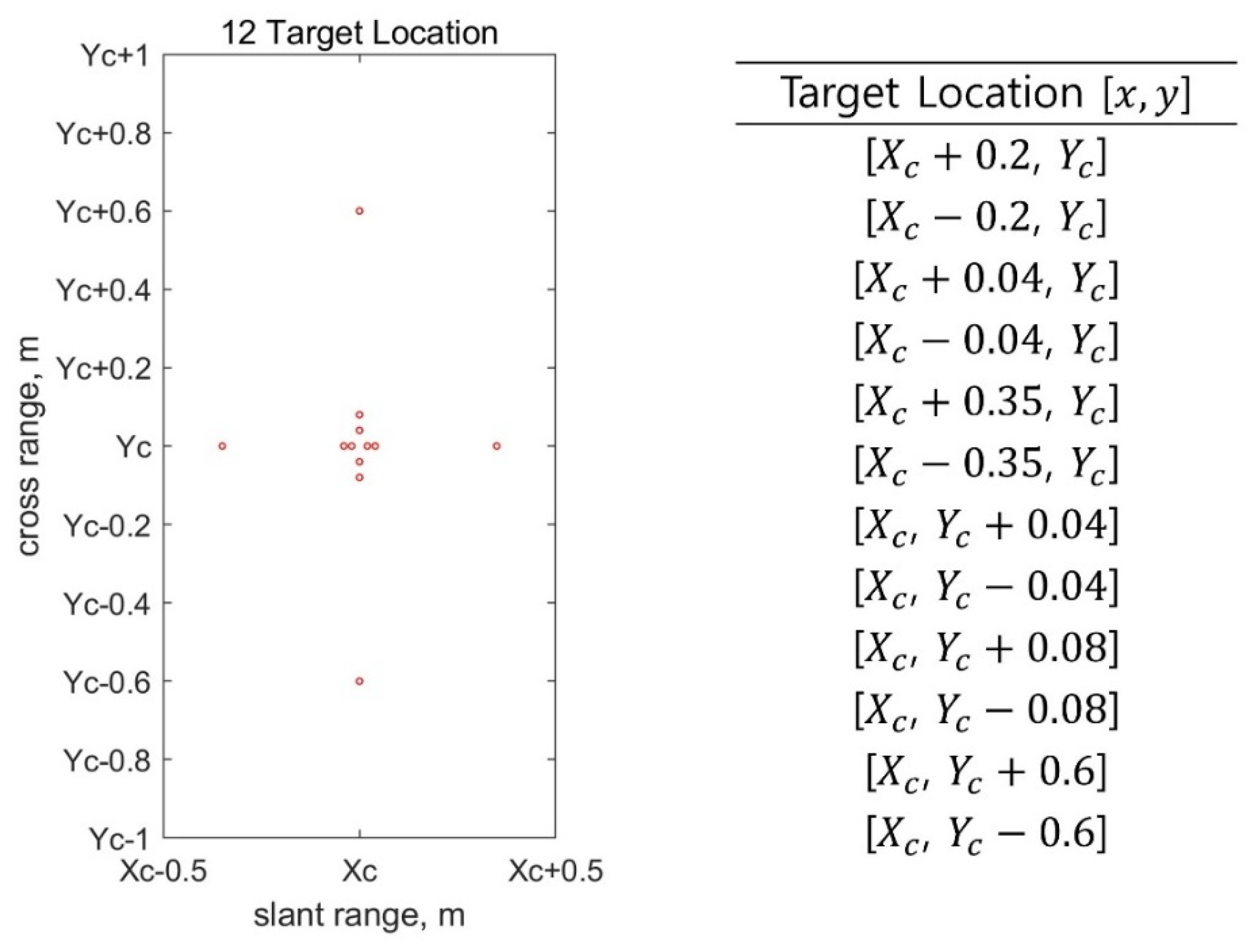
The ω-k and CS-SAS algorithms were compared for various cases. For the single-sensor SAS, five cases were simulated. The basic simulation environment was a single-sensor sonar operated at 0.02 m intervals from −5 to 5 in the cross-range axis, that is, Np = 501. The signal p(t) was a CW signal with carrier frequency fc = 400 kHz and pulse duration Tp = 0.1 ms. The center point of the area of interest was [Xc,Yc] = [250, 0], the half-size of the area of interest in slant-range was X0 = 0.5 m, the half-size of the area of interest in cross-range was Y0 = 1 m, the sampling frequency was fs = 50 kHz, and the area of interest consisted of NX = 101 and NY = 101 uniform grid points. The sound speed was c = 1500 m/s. Twelve-point targets were placed, as described in Figure 4.
All simulation environments for single-sensor sonar were fundamentally the same as the basic simulation environment described above and were performed by changing the noise level, Xc, fs, and sonar interval, as shown in Table 1.
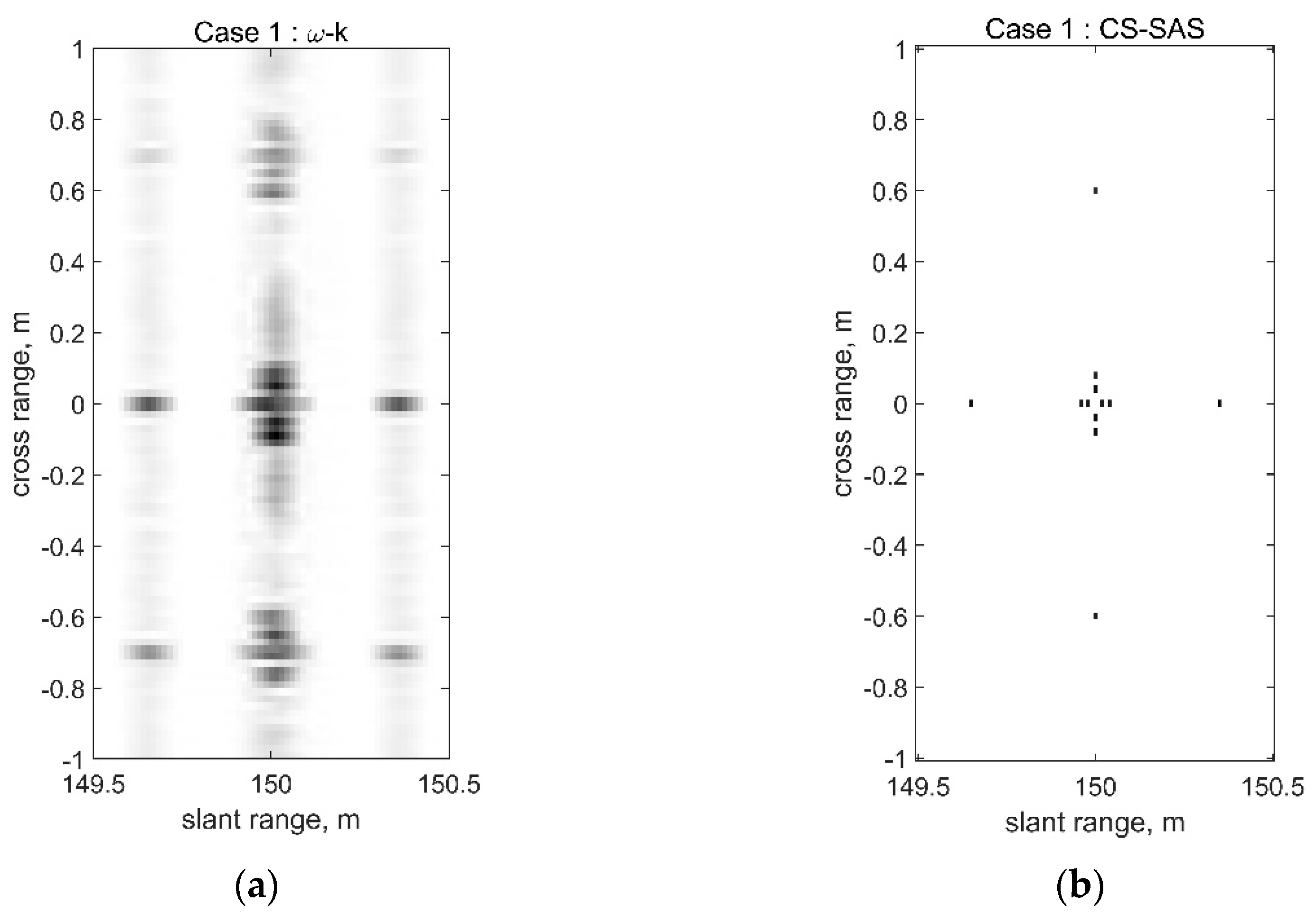
- Case 1
As shown in Figure 5, it was confirmed that the images obtained through the CS-SAS algorithm accurately distinguished 12 targets and had a good azimuth resolution. In addition, it was confirmed that there was no performance degradation caused by the side lobes. However, the result for the ω-k algorithm is unable to distinguish between targets adjacent to each other in the center of the area of interest. In addition, much aliasing occurs, especially in the azimuth direction. On account of the influence of matched filtering and Fourier transform, the exact position of the point targets cannot be obtained, resulting in a blurred result.
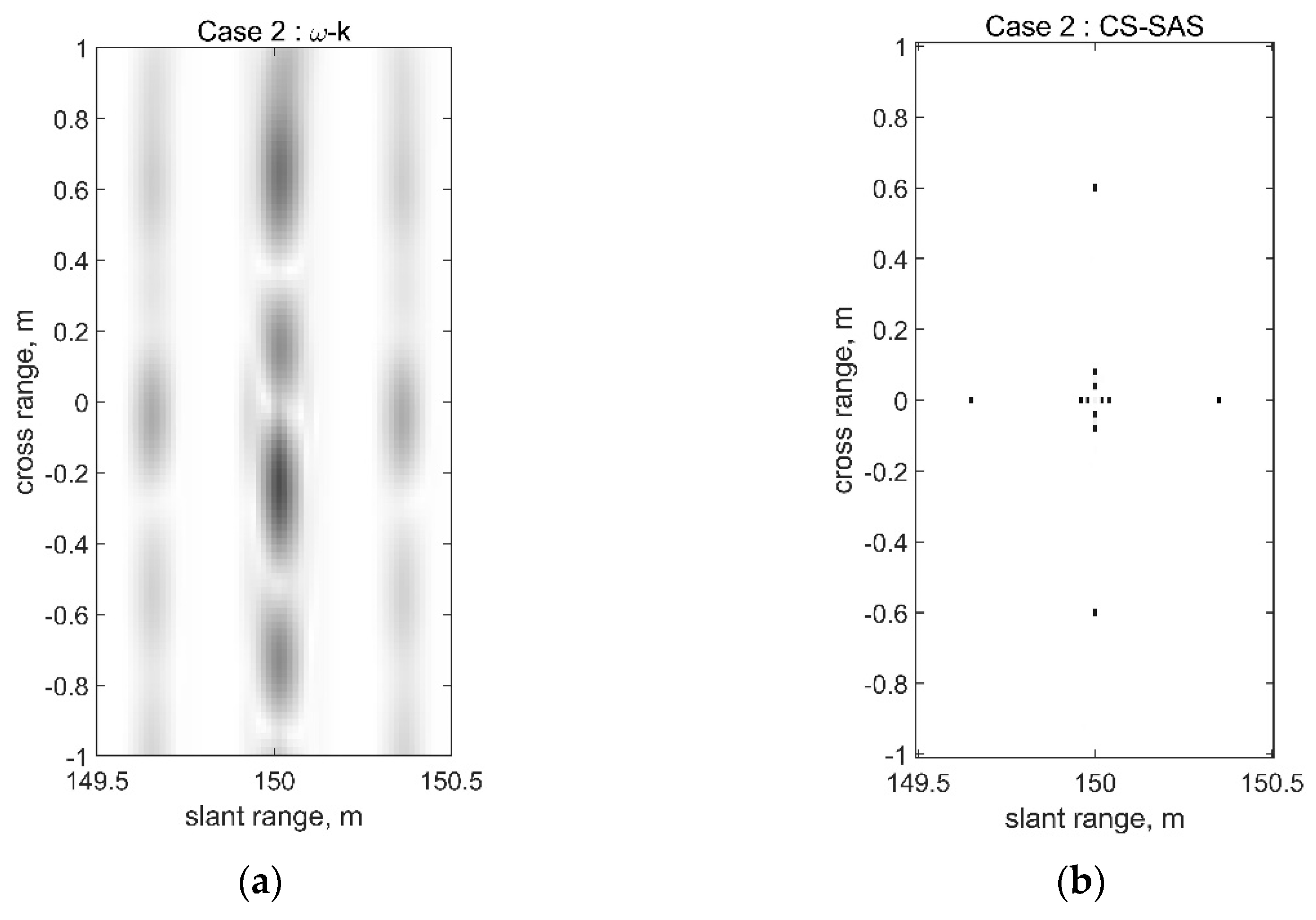
- Case 2
The results of the simulation are shown in Figure 6. In the case of the ω-k algorithm, because the sampling frequency is reduced by half compared to Case 1, the resolution in the slant-range direction is reduced. The aliasing at the center of the area of interest has a larger value than the values at the four target locations, [250 ± 0.02, 0] and [250 ± 0.04, 0]. Nonetheless, the image obtained using the CS-SAS algorithm yielded an accurate target image.
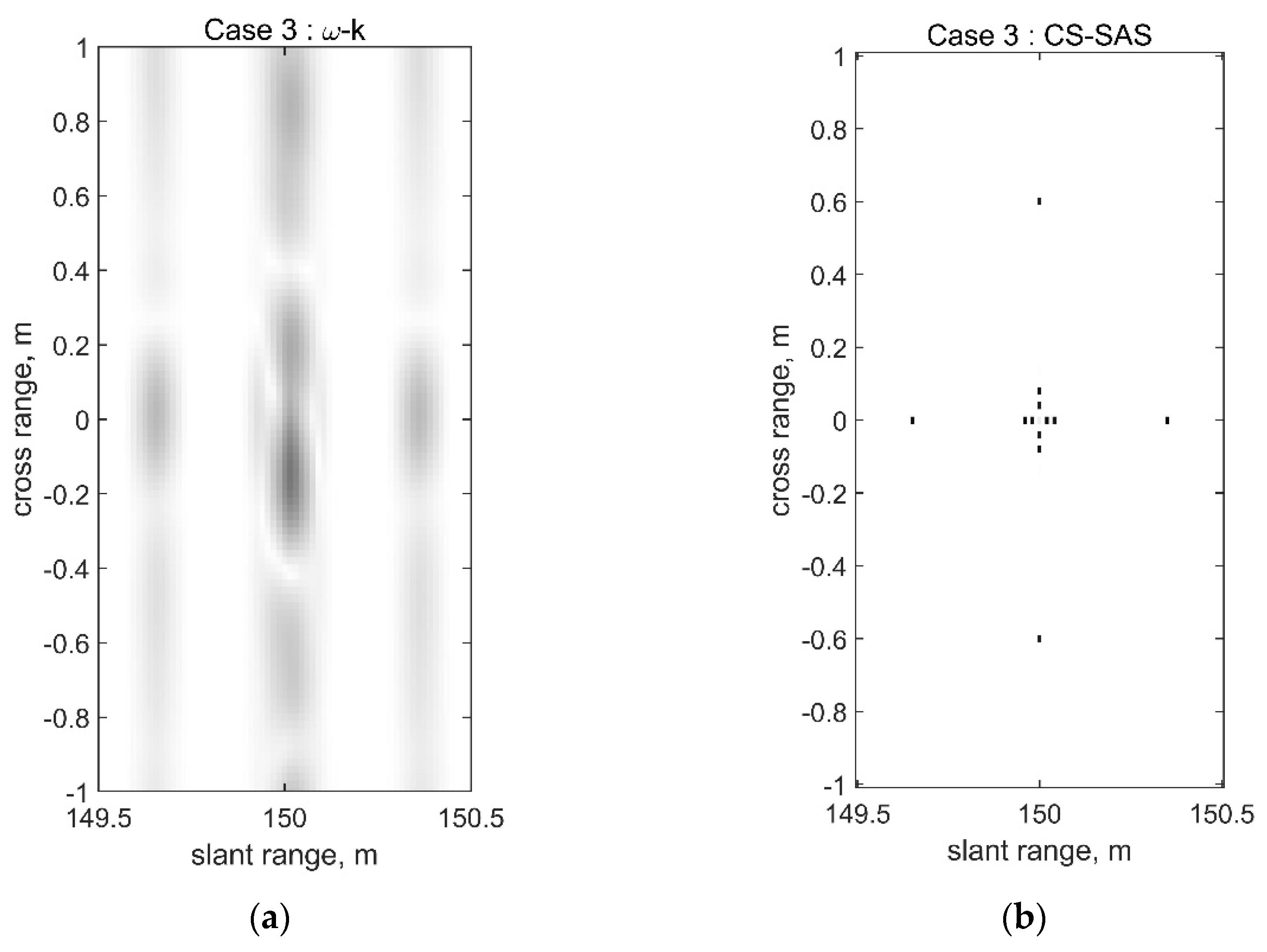
- Case 3
The results are shown in Figure 7. The CS-SAS algorithm accurately fetches the images of 12 targets. However, the ω-k algorithm requires a Fourier transform in the space domain, which violates Nyquist theory because the sampling level in the space domain is reduced to 1/10. Therefore, aliasing occurred, and the image of the target could not be properly obtained. The eight target points in the center were not distinguishable, and the remaining four points were difficult to determine.
- Case 4
The results are depicted in Figure 8. Even when the spatial sampling is reduced to a level of 1/20 and when some side lobes occur, the CS-SAS algorithm still fetches the image of 12 targets, whereas the ω-k algorithm fails to depict the proper image of the targets.
- Case 5
Noisy conditions with signal-to-noise ratios (SNRs) of 20, 10, and 5 dB were simulated. The results in Figure 9 indicate that the CS-SAS algorithm applied to an environment with SNRs of 20 dB and 10 dB, obtained an almost accurate image of the targets. However, when the SNR was 5 dB, the values at the grid point between [250, ±0.04] and [250, ±0.08] were greater than the values at [250, ±0.04] and [250, ±0.08], and an accurate image could not be obtained. As the noise became louder, a degree of degradation occurred. Nevertheless, the CS-SAS algorithm was still superior to the ω-k algorithm in terms of resolution and sidelobe suppression.
4.1.2. Simulation Results for Uniform Line Array
The CS-SAS and ω-k algorithms for a uniform line array were simulated in two cases. The first simulation case is as follows: The simulation environments of sampling frequency fs and sound velocity c, excluding sonar configuration and Xc, are the same as those of simulation Case 1 for a single sensor. The array has 20 receivers, with a 0.04 m spacing between receivers, as shown in Figure 10a. By moving 0.4 m between pings, a total of 25 pings were shot. The source position of the uniform line array is 0.1 m away from the first sensor in the cross-range direction. Conditions for other simulations are the same as for Case 1, except that the sensor spacing of the array is different. The array has two receivers, with 0.4 m spacing between receivers, as shown in Figure 10b. By moving 0.4 m between pings, a total of 25 pings were shot. The source position of the uniform line array is 0.1 m away from the first sensor in the cross-range direction.
- Case 1
The results for Case 1 are shown in Figure 11. The CS-SAS algorithm accurately fetched images of the 12 targets. Contrarily, the result for the ω-k algorithm showed aliasing. In particular, the total number of sensors used were 500 = 20 × 25, which compares favorably to the simulation environment of a single sensor; however, the interval between the sensors doubled to 0.04, and the spatial sampling interval also doubled, resulting in aliasing near [250, ±0.07].
- Case 2
The results for Case 2 are shown in Figure 12. The synthetic aperture is the same as in Case 1, but the sensor spacing is increased 10 times. Severe aliasing occurred in the ω-k results as well as the inability to properly identify the targets. However, the CS-SAS algorithm was significantly better distinguished.
The performances of the CS-SAS and ω-k algorithms were compared using simulation results for a single sensor and uniform line array. In the case of the ω-k algorithm, even under the most naïve simulation conditions, adjacent targets could not be distinguished and aliasing occurred, whereas in the case of the proposed algorithm, because CS was applied and sidelobes were rather suppressed, high-resolution results were obtained. In effect, CS-SAS has clearly distinguished targets under harsher conditions by increasing spatial sampling or reducing fs, and has obtained accurate locations and shown robustness in noisy situations. This is possible because the measured signal can be expressed in a sparse representation for a certain domain, and CS can significantly lower the sampling rate and has robust resistance to noise [36,39].
4.2. Experimental Data Results
This was a water tank experiment conducted by SonaTech Inc. (Santa Barbara, CA, USA). As shown in Figure 13a, an experiment was performed to obtain images of two rings in a water tank. As shown in Figure 13b, the sonar has one transmitter and 32 receivers. After transmitting and receiving the signal once, the transmitter moves 616.5 mm and then sends and receives the next signal. This process was repeated seven times to receive signals from 224 locations. The ping signal p(t) is a CW signal with carrier frequency fc = 455 kHz and pulse duration Tp = 0.3 ms, the sampling frequency is fs = 50 kHz, and the sound speed c = 1480 m/s. There are two ring-shaped targets of approximate length of major axis 1.5 m each in the slant-range of 7 to 10 m and a cross-range of −2.4385 to 2.4385 m.
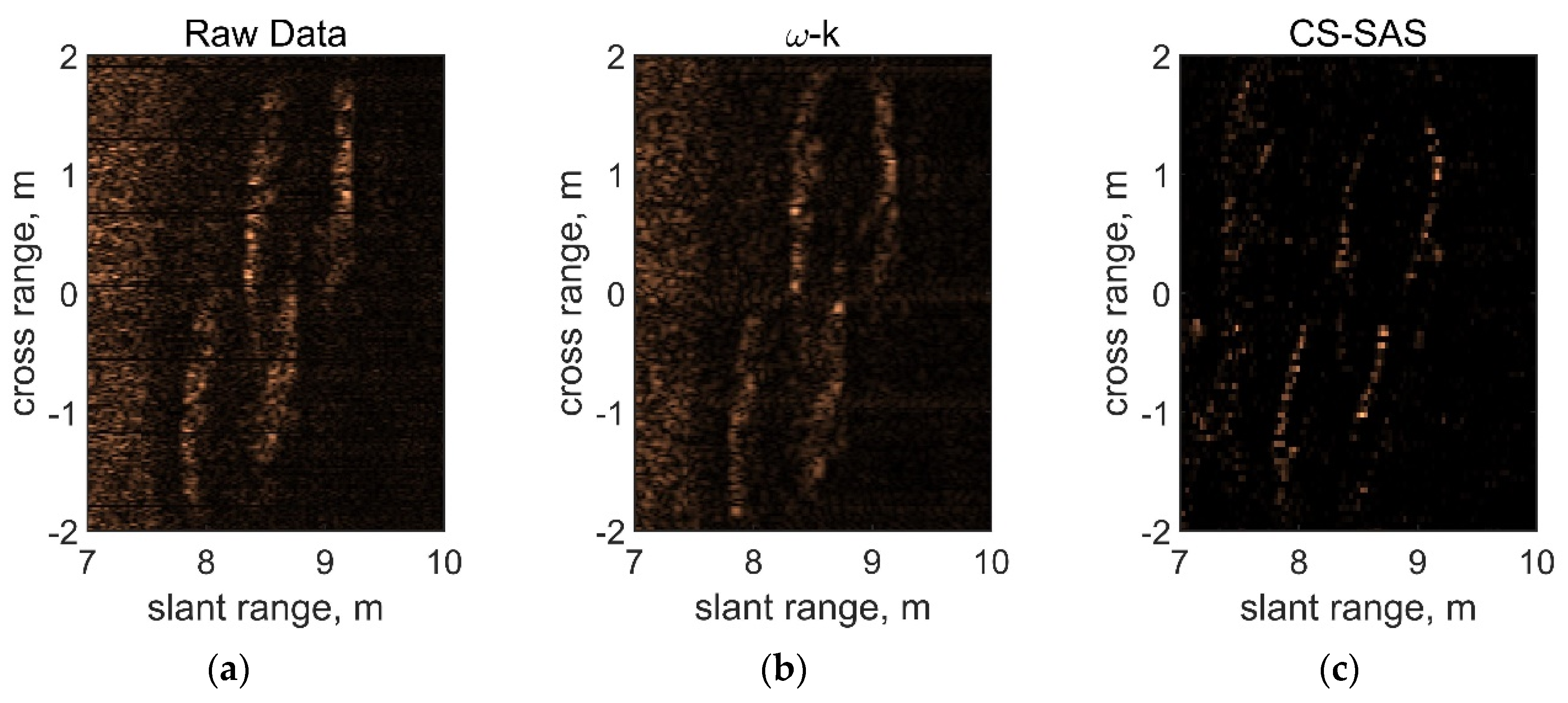
The raw data recorded in the slant-range are shown in Figure 14a. The CS-SAS result was derived by dividing the area of interest into a uniform grid of NX = 101 and NY = 101. The results of the ω-k and CS-SAS algorithms are shown in Figure 14b,c, respectively.
From the raw data, the targets can be seen in the form of rings, but the shape appears thick, and it is difficult to accurately determine the location of the targets. In the results of the ω-k algorithm, the shapes are slightly thinner, but aliasing is severe in the azimuth direction, and it appears that there are several rings. The results of the CS-SAS algorithm construct tworing-shaped targets. Because the CS-SAS algorithm attempts to bring an image with as little target distribution as possible, the side lobes are suppressed to obtain thin ring-shaped targets.
To examine whether the CS-SAS algorithm is robust under conditions where some of the sensors are broken, the result was derived by assuming a situation in which data from some sensors were lost. The experiment was divided into two cases: one case where the sensor failed uniformly (Sensor Loss: Uniform, SLU) and another case where the sensor failed randomly (Sensor Loss: Random, SLR). The percentages of sensors that did not malfunction and operated normally are also indicated in the results. The results are displayed in Figure 15.
In addition, peak signal-to-noise ratio (PSNR) and structural similarity index measure (SSIM), which are representative image quality measurement indicators [40,41], were calculated for quantitative comparison. PSNR is an index that evaluates loss information for the quality of the generated or compressed images and is expressed by the peak signal/mean square error (MSE) term. It has a unit of dB, and a higher value indicates less loss, i.e., higher image quality. SSIM is an index designed to evaluate differences in human visual quality rather than numerical errors. SSIM quality is evaluated in three aspects: luminance, contrast, and structural. However, since the correct answer image is not known, PSNR and SSIM were calculated for all sensor loss situations using Figure 14c as a reference image. The calculation results are shown in Table 2.
In the case of some conventional methods such as ω-k, a Fourier transform in space is performed. Therefore, it is difficult to obtain results freely in the form of an array because linear sampling is not possible in space when some sensors in the array fail. However, the CS-SAS algorithm does not perform Fourier transform in space and has a formulation that is free in the form of an array and, therefore, it is easy to obtain a result in a sensor loss situation. In addition, it is difficult to detect significant performance degradation of up to 75% for both SLU and SLR, and 50% of the SLR show particularly good results; note that CS has the best performance for random array or random down sampling [42,43]. Table 2 also shows that the random array results are generally better. In Table 2, it can be seen that the image quality of SLR is high for both 50% and 25%. At 75%, the indicators of SLR are worse than at 75% of SLU. Because there is little deterioration in image quality in 75% of cases, it can be seen that the PSNR and SSIM simply show how similar the reconstruction results are to Figure 14c, rather than showing the results of image quality deterioration. When it reaches approximately 25%, both SLU and SLR seem to blur to some extent, but in terms of side lobe suppression, it still shows no inferiority over the ω-k algorithm.
Using the CS-SAS algorithm in this study made it possible to obtain a higher resolution image than when using the conventional synthetic aperture sonar algorithm—the ω-k algorithm—and made it possible to reduce the problem of aliasing which also occurs in the conventional method. In addition, even with less spatial sampling, better results were obtained than compared to the conventional algorithm, and it was confirmed to be robust even when some sensors failed. Good results can be expected even if the number of sensors are reduced during actual sonar operation, and as a consequence, cost reduction is possible. Moreover, it is durable because it presents robust characteristics in failure situations. Results of actual experimental data were also observed, and it is expected that satisfying results will be obtained in the event that the CS-SAS algorithm is applied to a natural underwater environment.
5. Conclusions
In this paper, we proposed an algorithm that applies compressive sensing (CS) to a synthetic aperture sonar (SAS) under the assumption that the target distribution in water is sparse. Through simulation, it was confirmed that the proposed algorithm produces images with better resolution than the conventional SAS algorithm, the ω-k algorithm. In addition, because images obtained by the proposed method present very few and small side lobes, no deterioration of imaging performance occurs. Furthermore, even in the case of sampling at a low level that violates Nyquist theory in the time and space domain, a higher quality target image was obtained than with the ω-k algorithm.
Real environment applicability was revealed for the proposed method when comparing the results with actual experimental data. The results confirm that aliasing is reduced and side lobes are suppressed when applying the compressive sensing method. Contrarily, the ω-k algorithm does not obtain accurate target images due to aliasing. Importantly, it was confirmed that the proposed method is robust in the event of some sensors of the sonar system failing or when some data are lost.
Author Contributions
Conceptualization, H.-m.C. and H.-s.Y.; methodology, H.-m.C.; software, H.-m.C.; validation, H.-s.Y. and W.-j.S.; formal analysis, H.-m.C.; investigation, H.-m.C.; resources, H.-s.Y. and W.-j.S.; data curation, H.-m.C.; writing—original draft preparation, H.-m.C.; writing—review and editing, H.-s.Y. and W.-j.S.; visualization, H.-m.C.; supervision, W.-j.S.; project administration, H.-s.Y.; funding acquisition, W.-j.S. All authors have read and agreed to the published version of the manuscript.
Funding
This research received no external funding.
Data Availability Statement
The data presented in this study are not publicly available because these data belong to SonaTech Inc.
Acknowledgments
This research was supported by the Agency for Defense Development in Korea under Contract No. UD190005DD and the SonaTech Inc under Contract No. C180005.
Conflicts of Interest
The authors declare no conflict of interest.
References
- Soumekh, M. Synthetic Aperture Radar Signal. Processing with MATLAB Algorithms, 1st ed.; Wiley-Interscience: New York, NY, USA, 1999. [Google Scholar]
- Michael, P.H.; Peter, T.G. Synthetic Aperture Sonar: A Review of Current Status. IEEE J. Ocean. Eng. 2009, 34, 207–224. [Google Scholar]
- Hyun, A. A Study on Robust Synthetic Aperture Sonar Signal Processing for Multipath Environment using SAGE Algorithm. Ph.D. Thesis, Seoul National University, Seoul, Korea, 2016. [Google Scholar]
- Gustafson, E.; Jalving, B. HUGIN 1000 Arctic Class AUV. In Proceedings of the OTC Arctic Technology Conference, Houston, TX, USA, 7–9 February 2011. [Google Scholar]
- Hansen, R.E. Introduction to Synthetic Aperture Sonar. In Sonar Systems; Kolev, N.Z., Ed.; IntechOpen: Rijeka, Croatia, 2011; Chapter 1; pp. 3–28. [Google Scholar]
- Gough, P.T.; Hawkins, D.W. Unified Framework for Modern Synthetic Aperture Imaging Algorithms. Int. J. Imaging Syst. Technol. 1997, 8, 343–358. [Google Scholar] [CrossRef]
- Barber, B.C. Theory of Digital Imaging from Orbital Synthetic-Aperture Radar. Int. J. Remote Sens. 1985, 6, 1009–1057. [Google Scholar] [CrossRef]
- Bamler, R. A Comparison of Range-Doppler and Wavenumber Domain SAR Focusing Algorithms. IEEE Trans. Geosci. Remote Sens. 1992, 30, 706–713. [Google Scholar] [CrossRef]
- Cafforio, C.; Prati, C.; Rocca, F. SAR Data Focusing using Seismic Migration Techniques. IEEE Trans. Aerosp. Electron. Syst. 1991, 27, 194–207. [Google Scholar] [CrossRef]
- Stolt, R.H. Migration by Fourier Transform. Geophysics 1978, 43, 23–48. [Google Scholar] [CrossRef]
- Cumming, I.; Wong, F.; Raney, K. A SAR Processing Algorithm with No Interpolation. In Proceedings of the Geoscience and Remote Sensing Symposium, Houston, TX, USA, 26–29 May 1992; pp. 376–379. [Google Scholar]
- Marston, T.M.; Marston, P.L.; Williams, K.L. Scattering Resonances, Filtering with Reversible SAS Processing, and Applications of Quantitative Ray Theory. In Proceedings of the OCEANS MTS/IEEE, Seattle, WA, USA, 20–23 September 2010; pp. 1–9. [Google Scholar]
- Synnes, S.; Hunter, A.J.; Hansen, R.E.; Sæbø, T.O.; Callow, H.J.; Vossen, R.V.; Austeng, A. Wideband Synthetic Aperture Sonar Backprojection with Maximization of Wavenumber Domain Support. IEEE J. Oceanic Eng. 2017, 42, 880–891. [Google Scholar] [CrossRef] [Green Version]
- Elad, M. Sparse and Redundant Representations: From Theory to Applications in Signal. and Image Processing, 2nd ed.; Springer: New York, NY, USA, 2010; pp. 1–359. [Google Scholar]
- Krueger, K.R.; McClellanm, J.H.; Scott, W.R. Efficient Algorithm Design for GPR Imaging of Landmines. IEEE Trans. Geosci. Remote Sens. 2015, 53, 4010–4021. [Google Scholar] [CrossRef]
- Aberman, K.; Eldar, Y.C. Sub-Nyquist SAR via Fourier Domain Range Doppler Processing. IEEE Trans. Geosci. Remote Sens. 2017, 55, 6228–6244. [Google Scholar] [CrossRef] [Green Version]
- Lustig, M.; Donoho, D.L.; Pauly, J.M. Sparse MRI: The Application of Compressed Sensing for Rapid MR Imaging. Magn. Reson. Med. 2007, 58, 1182–1195. [Google Scholar] [CrossRef]
- Lustig, M.; Donoho, D.L.; Santos, J.M.; Pauly, J.M. Compressed Sensing MRI. IEEE Signal. Process. Mag. 2008, 25, 72–82. [Google Scholar] [CrossRef]
- Haupt, J.; Bajwa, W.U.; Raz, G.; Nowak, R. Toeplitz Compressed Sensing Matrices with Applications to Sparse Channel Estimation. IEEE Trans. Inf. Theory 2010, 56, 5862–5875. [Google Scholar] [CrossRef]
- Tur, R.; Eldar, Y.C.; Friedman, Z. Innovation Rate Sampling of Pulse Streams with Application to Ultrasound Imaging. IEEE Trans. Signal. Process. 2011, 59, 1827–1842. [Google Scholar] [CrossRef] [Green Version]
- Xenaki, A.; Gerstoft, P. Compressive Beamforming. J. Acoust. Soc. Am. 2014, 136, 260–271. [Google Scholar] [CrossRef] [Green Version]
- Gerstoft, P.; Xenaki, A.; Mecklenbräuker, C.F. Multiple and Single Snapshot Compressive Beamforming. J. Acoust. Soc. Am. 2015, 138, 2003–2014. [Google Scholar] [CrossRef] [Green Version]
- Güven, H.E.; Güngör, A.; Ҫetin, M. An Augmented Lagrangian Method for Complex-Valued Compressed SAR Imaging. IEEE Trans. Comput. Imag. 2016, 2, 235–250. [Google Scholar] [CrossRef]
- Güngör, A.; Ҫetin, M.; Güven, H.E. Autofocused Compressive SAR Imaging based on the Alternating Direction Method of Multipliers. In Proceedings of the 2017 IEEE Radar Conference, Seattle, WA, USA, 8–12 May 2017; pp. 1573–1576. [Google Scholar]
- Zhao, B.; Huang, L.; Zhang, J. Single Channel SAR Deception Jamming Suppression via Dynamic Aperture Processing. IEEE Sens. J. 2017, 17, 4225–4230. [Google Scholar] [CrossRef]
- Ҫetin, M.; Stojanović, I.; Önhon, Ö.; Varshney, K.; Samadi, S.; Karl, W.C.; Willsky, A.S. Sparsity-Driven Synthetic Aperture Radar Imaging: Reconstruction, Autofocusing, Moving targets, and Compressed Sensing. IEEE Signal. Process. Mag. 2014, 31, 27–40. [Google Scholar] [CrossRef]
- Amin, M. Compressive Sensing for Urban. Radar, 1st ed.; CRC Press: Boca Raton, FL, USA, 2014. [Google Scholar]
- Wei, S.J.; Zhang, X.L.; Shi, J.; Xiang, G. Sparse Reconstruction for SAR Imaging Based on Compressed Sensing. Prog. Electromagn. Res. 2010, 109, 63–81. [Google Scholar] [CrossRef] [Green Version]
- Leier, S.; Zoubir, A.M. Aperture Undersampling using Compressive Sensing for Synthetic Aperture Stripmap Imaging. EURASIP J. Adv. Signal. Process. 2014, 156. [Google Scholar] [CrossRef] [Green Version]
- Xenaki, A.; Pailhas, Y. Compressive Synthetic Aperture Sonar Imaging with Distributed Optimization. J. Acoust. Soc. Am. 2019, 146, 1839–1850. [Google Scholar] [CrossRef] [PubMed] [Green Version]
- Ji, X.; Zhou, L.; Cong, W. Effect of Incorrect Sound Velocity on Synthetic Aperture Sonar Resolution. In Proceedings of the 2019 MATEC Web Conf. 2019, Sibiu, Romania, 5–7 June 2019. [Google Scholar] [CrossRef]
- Cutrona, L.J. Comparison of Sonar System Performance Achievable using Synthetic-Aperture Techniques with the Performance Achievable by More Conventional Means. J. Acoust. Soc. Am. 1975, 58, 336–348. [Google Scholar] [CrossRef]
- Cutrona, L.J. Additional Characteristics of Synthetic-Aperture Sonar Systems and a Further Comparison with Nonsynthetic-Aperture Sonar Systems. J. Acoust. Soc. Am. 1977, 61, 1213–1217. [Google Scholar] [CrossRef]
- Soumekh, M. Fourier Array Imaging; Prentice-Hall: Hoboken, NJ, USA, 1994. [Google Scholar]
- Gough, P.T.; Hawkins, D.W. Imaging Algorithms for a Strip-Map Synthetic Aperture Sonar: Minimizing the Effects of Aperture Errors and Aperture Undersampling. IEEE J. Ocean. Eng. 1997, 22, 27–39. [Google Scholar] [CrossRef]
- Donoho, D.L. Compressed Sensing. IEEE Trans. Inf. Theory. 2006, 52, 1289–1306. [Google Scholar] [CrossRef]
- Grant, M.; Boyd, S.; Ye, Y. CVX: Matlab Software for Disciplined Convex Programming. Available online: http://cvxr.com/cvx (accessed on 1 December 2020).
- Baraniuk, R.G.; Cevher, V.; Duarte, M.; Hegde, C. Model-Based Compressive Sensing. IEEE Trans. Inf. Theory 2010, 56, 1982–2001. [Google Scholar] [CrossRef] [Green Version]
- Candes, E.J.; Romberg, J.; Tao, T. Robust Uncertainty Principles: Exact Signal Reconstruction from Highly Incomplete Frequency Information. IEEE Trans. Inf. Theory 2006, 52, 489–509. [Google Scholar] [CrossRef] [Green Version]
- Horè, A.; Ziou, D. Image Quality Metrics: PSNR vs. SSIM. In Proceedings of the 2010 20th International Conference on Pattern Recognition, Istanbul, Turkey, 23–26 August 2010; pp. 2366–2369. [Google Scholar]
- Rehman, A.; Wang, Z. Reduced–Reference SSIM Estimation. In Proceedings of the 2010 IEEE 17th International Conference on Image Processing, Hong Kong, China, 26–29 September 2010; pp. 289–292. [Google Scholar]
- Baraniuk, R.G. Compressive Sensing [Lecture Notes]. IEEE Signal. Process. Mag. 2007, 24, 118–121. [Google Scholar] [CrossRef]
- Baraniuk, R.; Davenport, M.; DeVore, R.; Wakin, M. A Simple Proof of the Restricted Isometry Property for Random Matrices. Constr. Approx. 2008, 28, 253–263. [Google Scholar] [CrossRef] [Green Version]
Figure 1.
SAS geometry.

Figure 2.
Flow chart of the ω-k algorithm.

Figure 3.
Description for a single sensor sonar operation: um is the single sensor corresponding to the m-th ping, Np is the total number of pings, σk is a virtual target, Nx is the number of the grid in the x direction, Ny is the number of the grid in the y direction, (Xc,Yc) is the center point of the area of interest, X0 is the half-size of the area of interest in the x direction, Y0 is the half-size of the area of interest in the y direction.

Figure 4.
Locations of the 12 targets.

Figure 5.
Simulation results for Case 1 for single sensor: (a) result for the ω-k algorithm; (b) result for the CS-SAS algorithm for single sensor.
Figure 5.
Simulation results for Case 1 for single sensor: (a) result for the ω-k algorithm; (b) result for the CS-SAS algorithm for single sensor.

Figure 6.
Simulation results for Case 2 for single sensor: (a) result for the ω-k algorithm; (b) result for the CS-SAS algorithm for single sensor.
Figure 6.
Simulation results for Case 2 for single sensor: (a) result for the ω-k algorithm; (b) result for the CS-SAS algorithm for single sensor.

Figure 7.
Simulation results for Case 3 for single sensor: (a) result for the ω-k algorithm; (b) result for the CS-SAS algorithm for single sensor.
Figure 7.
Simulation results for Case 3 for single sensor: (a) result for the ω-k algorithm; (b) result for the CS-SAS algorithm for single sensor.

Figure 8.
Simulation results for Case 4 for single sensor: (a) result for the ω-k algorithm; (b) result for the CS-SAS algorithm for single sensor.
Figure 8.
Simulation results for Case 4 for single sensor: (a) result for the ω-k algorithm; (b) result for the CS-SAS algorithm for single sensor.

Figure 9.
Simulation results of CS-SAS algorithm for Case 5 for single sensor: (a) SNR = 20 dB; (b) SNR = 10 dB; (c) SNR = 5 dB.
Figure 9.
Simulation results of CS-SAS algorithm for Case 5 for single sensor: (a) SNR = 20 dB; (b) SNR = 10 dB; (c) SNR = 5 dB.

Figure 10.
Description of line array in: (a) the first case of simulation; (b) the second case of simulation; the red box is a transmitter, and the black boxes are receivers. The black-dash boxes in (b) are actually empty but marked for comparison with (a).
Figure 10.
Description of line array in: (a) the first case of simulation; (b) the second case of simulation; the red box is a transmitter, and the black boxes are receivers. The black-dash boxes in (b) are actually empty but marked for comparison with (a).

Figure 11.
Simulation results for Case 1 for uniform line array: (a) result for the ω-k algorithm; (b) result for the CS-SAS algorithm for uniform line array.
Figure 11.
Simulation results for Case 1 for uniform line array: (a) result for the ω-k algorithm; (b) result for the CS-SAS algorithm for uniform line array.

Figure 12.
Simulation results for Case 2 for uniform line array: (a) result for the ω-k algorithm; (b) result for the CS-SAS algorithm for a uniform line array.
Figure 12.
Simulation results for Case 2 for uniform line array: (a) result for the ω-k algorithm; (b) result for the CS-SAS algorithm for a uniform line array.

Figure 13.
Water tank experiment overview: (a) water tank structure; (b) synthetic aperture line-array sonar.
Figure 13.
Water tank experiment overview: (a) water tank structure; (b) synthetic aperture line-array sonar.

Figure 14.
(a) Raw data; (b) result for the ω-k algorithm; (c) result for the CS-SAS algorithm.

Figure 15.
Results for some sensor loss conditions. Uniformly broken case (SLU) where the percentage of the remaining sensors are: (a) 75%; (b) 50%; (c) 25%. Randomly broken case (SRU) where the percentage of the remaining sensors are (d) 75%; (e) 50%; (f) 25%.
Figure 15.
Results for some sensor loss conditions. Uniformly broken case (SLU) where the percentage of the remaining sensors are: (a) 75%; (b) 50%; (c) 25%. Randomly broken case (SRU) where the percentage of the remaining sensors are (d) 75%; (e) 50%; (f) 25%.


Table 1.
Simulation Case for Single Sensor.
| Case | Noise Existence | Xc (m) | fs (kHz) | Sonar Interval (m) |
|---|---|---|---|---|
| 1 | X | 250 | 50 | 0.02 |
| 2 | X | 250 | 25 | 0.02 |
| 3 | X | 150 | 50 | 0.2 |
| 4 | X | 150 | 50 | 0.4 |
| 5 | O | 250 | 50 | 0.02 |
Table 2.
PSNR and SSIM.
| SLU 75% | SLU 50% | SLU 25% | |
| PSNR (dB) | 33.7691 | 29.2229 | 28.1871 |
| SSIM | 0.8850 | 0.6947 | 0.6029 |
| SLR 75% | SLR 50% | SLR 25% | |
| PSNR (dB) | 32.9409 | 30.6011 | 28.4189 |
| SSIM | 0.8609 | 0.7324 | 0.6178 |
Publisher’s Note: MDPI stays neutral with regard to jurisdictional claims in published maps and institutional affiliations. |
© 2021 by the authors. Licensee MDPI, Basel, Switzerland. This article is an open access article distributed under the terms and conditions of the Creative Commons Attribution (CC BY) license (https://creativecommons.org/licenses/by/4.0/).
Share and Cite
MDPI and ACS Style
Choi, H.-m.; Yang, H.-s.; Seong, W.-j. Compressive Underwater Sonar Imaging with Synthetic Aperture Processing. Remote Sens. 2021, 13, 1924. https://0-doi-org.brum.beds.ac.uk/10.3390/rs13101924
AMA Style
Choi H-m, Yang H-s, Seong W-j. Compressive Underwater Sonar Imaging with Synthetic Aperture Processing. Remote Sensing. 2021; 13(10):1924. https://0-doi-org.brum.beds.ac.uk/10.3390/rs13101924
Chicago/Turabian StyleChoi, Ha-min, Hae-sang Yang, and Woo-jae Seong. 2021. "Compressive Underwater Sonar Imaging with Synthetic Aperture Processing" Remote Sensing 13, no. 10: 1924. https://0-doi-org.brum.beds.ac.uk/10.3390/rs13101924
Note that from the first issue of 2016, this journal uses article numbers instead of page numbers. See further details here.