Communication

Centroid Error Analysis of Beacon Tracking under Atmospheric Turbulence for Optical Communication Links

Korea Astronomy and Space Science Institute, Space Science Division, Daejeon 34055, Korea
*
Author to whom correspondence should be addressed.
Remote Sens. 2021, 13(10), 1931; https://0-doi-org.brum.beds.ac.uk/10.3390/rs13101931
Submission received: 23 March 2021 / Revised: 7 May 2021 / Accepted: 13 May 2021 / Published: 15 May 2021
(This article belongs to the Special Issue Space LiDAR Technologies and Applications)

Abstract

:
Optical satellite communication has received considerable attention as a promising alternative to radio frequency communication because of its potential advantages including higher data rates and license free spectrum. Many studies have conducted performance analyses of optical communication channels, but few have investigated beacon tracking channels under atmospheric turbulence. The centroid accuracy of beacon tracking channels is limited by not only noise sources, but also a finite delay time, which also fluctuates due to atmospheric turbulence. Consequently, the centroid error is an important figure of merit when evaluating the performance of a beacon tracking system. In this study, the closed-form expressions were derived for average centroid error and fade probability, based on received photoelectron counts depending on exposure time, taking into account the log-normal tracking channels. We analyzed the angular positioning performance of beacon tracking detectors onboard small satellites in the presence of atmospheric turbulence, in terms of centroid error and fade probability. We found that an optimal exposure time exists, which minimizes the centroid error, and that fade probability is inversely proportional to the exposure time. These are significant properties to consider in the design of beacon tracking systems.

Graphical Abstract

1. Introduction

Optical satellite communication has received significant attention as a promising advance in satellite communication, with the potential advantages of higher data rate, license free spectrum, better security, smaller size, lower mass, and lower power consumption [1,2,3,4,5]. Because of the extremely narrow optical beamwidth, a very precise beam steering system is required to ensure a reliable and stable optical communication link, since this is usually beyond the satellite’s body pointing capability. For this purpose, pointing, acquisition, and tracking (PAT) technology, considered one of the key technologies in optical satellite communication, must be employed to maintain an optical line-of-sight (LOS) between the transmitter and receiver, even in the face of pointing jitter caused by satellite platform vibrations and atmospheric turbulence. The PAT system is normally composed of three components that deal with different requirements: a coarse pointing assembly (CPA), a fine pointing assembly (FPA), and a point-ahead assembly (PAA).
The CPA provides wide angle steering, but is a low bandwidth mechanism for initial pointing and spatial acquisition. It employs wide dynamic range gimbals and wide field-of-view (FoV) image sensors, based on charge coupled device (CCD) or complementary metal–oxide–semiconductor (CMOS). The CCD and CMOS sensors allow a low frame rate, on the order of a dozen frames per second, even though they are capable of covering the uncertainty region of the receiver. With the use of a windowed readout mode for the array containing the beacon laser spots, the image sensors can also provide a sufficiently high frame rate and good positioning accuracy required for fine tracking [6,7,8].
The FPA detector provides not only more precise and faster LOS alignment, but also a narrower steering angle. To accomplish this, it employs a fast steering mirror and a position-sensitive detector such as quadrant PIN photodiode (QPD) or quadrant avalanche photodiode (QAPD). The position-sensitive detectors have several advantages over classical image sensors including better positioning accuracy, a faster response time, and very simple signal conditioning circuits [9]. The CPA have to be able to control several-centimeter-class telescopes within a pointing accuracy of sub-micro radians for planetary missions, or several micro radians for Earth orbiting missions, and its bandwidth should also be larger than 1 kHz to accommodate the pointing jitters caused by the satellite platform vibration and atmospheric turbulence [4,8,10,11,12].
Because of the relative velocity of the two terminals and the finite speed of light, an angular offset exists between the transmitting and received beams, the so-called point-ahead angle. The magnitude of angular offset is achievable with the help of known ephemeris data, up to 70 micro radians for inter-satellite links and as much as 500 micro radians for interplanetary links [13,14,15]. The PAA compensates the point-ahead angle by controlling the fast steering mirror if the angle is comparable to or larger than the transmitting beamwidth. Figure 1 shows the block diagram of the optical communication terminal including the PAT system with two types of actuators: gimbal and fast steering mirror (FSM).
When a beacon beam propagates through the atmosphere, it can be adversely affected by atmospheric turbulence including atmospheric scintillation such as intensity and phase fluctuations, angle of arrival fluctuations, beam spot wandering, and spatial beam spreading [16,17,18]. The beacon image follows the point spread function of the imaging optics since the uplink beacon can be regarded as a point source rather than an extended object [19], which can be distorted and blurred by atmospheric turbulence. Therefore, the centroid error of beacon images on a beacon detector depends on atmospheric turbulence as well as the exposure time, which plays a great role in the signal-to-noise ratio (SNR).
The limited accuracy of beacon detectors has been analyzed in terms of the noise equivalent angle, known as the random centroid error [20,21,22], particularly in the field of adaptive optics to evaluate the Shack–Hartmann wavefront sensors [23,24,25,26,27]. However, the intensity fluctuations resulting from atmospheric turbulence were not taken into consideration in these reports to precisely assess the centroid error. Over the years, many mathematical models have been proposed to describe the turbulence-induced scintillation in terms of probability density functions including the log-normal, K-channel, negative exponential, and gamma–gamma models [28,29,30,31,32]. Specifically, the log-normal and gamma–gamma models are widely used due to their simplicity and good agreement between the theoretical and experimental data. Consequently, they have been found to be suitable for weak-to-moderate and moderate-to-strong turbulence conditions, respectively [33].
An accurate centroid estimation is critical to the beacon tracking system to point the optical beam toward the partner terminal, so that sufficient optical power is received to meet the data rate and bit error rate performance requirements. This makes it essential, when evaluating the pointing capability of a PAT system, to analyze the centroid error intrinsic to noise sources and the finite delay time under atmospheric turbulence.
Korea has a plan to conduct an optical downlink experiment employing a CubeSat that requires not only the use available commercial off-the-shelf (COTS) components for a reduction in development costs, but also accurate pointing and tracking capabilities under the size, weight, and power constraints for a reliable communication link. Thus, the beacon tracking system onboard a CubeSat should be designed through a trade-off between two requirements for COTS components as well as pointing and tracking capabilities over fade channels.
In this study, the SNR formula of position-sensitive detectors was given in terms of the received photoelectron count depending heavily on the exposure time, which also includes shot noise, background noise, dark current, and thermal noise. Taking into account the log-normal tracking channels, the closed-form models were derived for two metrics, average centroid error and fade probability in the function of the received photoelectron count. For practical applications, the received photon count was estimated by considering turbulence-induced beam spreading and atmospheric attenuation due to atmospheric constituents and cirrus clouds.
We analyzed the angular positioning performance of an uplink beacon system for two metrics in terms of exposure time and atmospheric turbulence strength using CMOS and QAPD detectors. We found from numerical simulations that an optimal exposure time exists, which minimizes the centroid error resulting from noise sources and the exposure time latency. However, fade probabilities decreased rapidly as the exposure time was extended and atmospheric turbulence became strong. These characteristics should be taken into account in a trade-off of the design of the beacon tracking system requiring high bandwidth and high positioning accuracy.

2. System and Channel Model

2.1. Link Equation

The link equation is widely used in communications to predict the power received at an optical detector, because it enables the analysis of the trade-offs between system parameters and channel performance. The intensity of a beacon beam is non-uniformly distributed in the spatial domain along the direction of beam propagation. Taking into account the non-uniform irradiance distribution and beam spreading due to atmospheric turbulence, the link equation is given by [18,34]
P R = 2 P T π W e f f 2 ( z ) η T η R A R T A T C exp [ 2 d 2 W e f f 2 ( z ) ] ,
where P T and P R are the transmitting and received optical powers, respectively; W e f f is the effective spot size including the beam divergence and spreading; z is the axial distance from the beam waist; η T is the transmitter optical efficiency; η R is the receiver optical efficiency including the optical filter transmittance; A R is the receiving area; d is the radial distance from the axis of beam propagation (i.e., d = z θ e for a small pointing error of θ e ); and T A and T C are the atmospheric attenuations produced by atmospheric constituents and cirrus clouds, respectively. The last term indicates the pointing loss due to LOS misalignment between the transmitter and the receiver.
The beacon beam suffers from power losses resulting from absorption and scattering by molecules and aerosols suspended in the atmosphere as well as cirrus clouds. The atmospheric attenuations resulting from the constituents and cirrus clouds are expressed as [35]
T A ( λ , V , h s ) = exp [ σ ( λ , V , 0 ) h S H sec ( θ Z ) exp ( h s h S H ) ] ,
T C = exp [ 0.14 ( C T sec θ Z ) 2 ] ,
where σ ( λ , V , 0 ) and V are the atmospheric attenuation coefficient and visibility at sea level, respectively, and λ is the beacon wavelength. h S H = 1.2 km is the scale height; θ Z is the zenith angle of the satellite; h s is the height of the optical ground station; and C T is the cirrus cloud thickness. It is worth noting that in the low elevation angle regimes, atmospheric attenuation by cirrus clouds is dominant compared to attenuation by atmospheric constituents.

2.2. Turbulence-Induced Beam Spreading

When the beacon beam propagates through the atmosphere, it undergoes beam spreading due to small-scale turbulent eddies, in addition to the far-field angular spreading coming from the divergence angle. This beam spreading makes the spot size larger, resulting in a reduction in beam irradiance at the detector. Assuming a Gaussian beam, the effective spot size is approximated in the uplink as follows [32]:
W e f f 2 ( z ) = W 2 ( z ) ( 1 + T ) ,
where
W ( z ) = W 0 1 + ( 2 z k W 0 2 ) 2 2 z k W 0 = z θ D ,
T = 4.35 k 7 / 6 ( Λ H ) 5 / 6 sec 11 / 6 ( θ z ) h s h s + H C n 2 ( h ) ( 1 h h s H ) 5 / 3 d h .
Here, T is the additional spreading caused by atmospheric turbulence; k is the optical wavenumber; W0 is the beam waist (i.e., beam size at z = 0 ); θ D is the far-field divergence half-angle of the beacon beam; Λ is the Fresnel ratio defined as Λ = 2 z / k W 2 ( z ) ; H is the difference in altitude between the receiver and the optical ground station at h s ; and C n 2 ( h ) is the refractive-index structure parameter, which characterizes the strength of atmospheric turbulence.
Many models have been proposed to predict the behavior of the refractive-index structure parameter, which is a quantitative measure of atmospheric turbulence. The Hufnagel–Valley model is widely used since it not only allows for easy variation of the day-time and night-time profile by adjusting various site parameters including wind speed, isoplanatic angle, and altitude, but is also best suited for ground-to-satellite uplink [4]. The model is given as
C n 2 ( h ) = 0.00594 ( v 27 ) 2 ( 10 5 h ) 10 exp ( h 1000 ) + 2.7 × 10 16 exp ( h 1500 ) + A 0 exp ( h 100 ) ,
where v is the mean square value of the wind speed in m / s , and A 0 is the nominal value of the refractive-index structure parameter at the ground in m 2 / 3 . It is noteworthy that the turbulence strength is dominated by A 0 near the ground, but by v at high altitude (i.e., h > 5 km ) [36]. The value of A 0 is typically in the range from 10 17 m 2 / 3 for weak turbulence to 10 12 m 2 / 3 for strong turbulence, with a typical average value being 10 15 m 2 / 3 [37].

2.3. Log-Normal Tracking Channel

The centroid accuracy of detectors including image sensors or position-sensitive detectors can be significantly degraded by beacon intensity fluctuations due to atmospheric turbulence over the tracking channel. Over the years, a number of statistical models have been introduced to describe intensity fluctuations of a propagated beam in terms of probability density function. The log-normal model is restricted to weak turbulence conditions with scintillation indexes of less than 1.0. Taking into account the exposure time, the average number of received beacon photoelectrons can be calculated as
K s = η Q λ P R c T s ,
where η Q is the quantum efficiency of the detector; T s is the exposure time in seconds; and and c are the Plank’s constant and light speed, respectively. Without loss of generality, K s can also be considered a log-normal distributed random variable instead of the received intensity. Therefore, the probability density function of the log-normal model is defined as [31]
f ( K s ) = 1 2 π σ k 2 K s exp ( ( ln K s m k ) 2 2 σ k 2 ) ,
where
m k = ln ( E [ K s ] ) σ k 2 2 ,
σ k 2 = ln ( σ s i 2 + 1 ) .
Here, m k and σ k 2 denote the mean and variance of ln ( K s ) , respectively, and σ s i 2 is the scintillation index to describe the intensity fluctuation. The scintillation index is expressed by various formulas depending on turbulence strength, wave types, and wave propagation path such as uplink, downlink, and horizontal path. In the case of both weak turbulence condition and uplink, σ s i 2 can be written for a spherical wave as [12]:
σ s i 2 = 2.24 k 7 / 6 sec 11 / 6 ( θ z ) h s h s + H C n 2 ( h ) ( H + h 0 h ) 5 / 6 ( 1 H + h s h H ) 5 / 6 d h .

3. Centroid Error Analysis

3.1. Signal-to-Noise Ratio

The centroid error can be estimated based on the image size as well as SNR, which is defined as the ratio of the signal photoelectron counts to the noise fluctuation intensity during the integration time [27]. The centroid accuracy is proportional to SNR, but various noise sources during the integration time may lead to significant degradation of the centroid accuracy. In the quantitative signal analysis of beacon images on the beacon tracking detector, the centroid algorithm is used to compute the beacon location within the centroid window, which should be carefully selected so as not to deteriorate the centroid accuracy. Assuming the background noise is uniformly distributed over each pixel, the CMOS sensor’s SNR corresponding to the exposure time is given by
γ C M O S ( K s ) = K s K s + N p ( N b T s + N d T s + N r 2 ) ,
where N p is the number of pixels involved in the centroid window; N d is the dark current in electrons per second per pixel; N r is the read noise in root-mean-square electrons per pixel; and N b is the background noise in photoelectrons per second per pixel and can be calculated from η Q λ P b / c N F o V , where N F o V is the number of pixels corresponding to the FPA detector’s FoV, and P b is the received power from background radiance. Note that the SNR equation for the CCD detector is exactly the same as for the CMOS detector. The background power is given by [4]
P b = L λ Ω F o V η R A R Δ λ f i l t e r ,
where L λ is the background spectral radiance; Ω F o V is the detector FoV in steradians; and Δ λ f i l t e r is the optical bandwidth.
A quadrant position-sensitive detector consists of four individual yet identical photodiodes, and each quadrant generates an output photocurrent that is proportional to the amount of incident optical power, depending on the beam spot position and shape on the photodiode surface. Because of these properties, it provides continuous positioning data, higher positioning accuracy, and high-speed response. Unlike QPD detectors, QAPD detectors are used to detect the position of a faint beacon spot due to its high sensitivity. Assuming the responsivity and dark current are the same in each quadrant, the QAPD detector’s SNR corresponding to the exposure time is derived as
γ Q A P D ( K s ) = K s F K s + 4 ( F G 2 N b T s + N d T s + σ n 2 T s / q 2 ) / G 2 ,
where F is the excess noise factor, and G is the gain. N d is the APD dark current consisting of two components (i.e., surface dark current I d s and bulk dark current I d b ), which can be calculated from the equation ( F G 2 I d b + I d s ) / q , because the surface dark current does not trigger an avalanche process within the substrate but the bulk dark current does [38]. σ n 2 is the thermal noise, defined as 2 k B T / R L , where k B is the Boltzmann constant; T is the absolute temperature; and R L is the load resistance of the detector circuit. Note that we can also get the SNR equation of the QPD detector from Equation (15) by taking F = 1 and G = 1 .

3.2. Centroid Error under Atmospheric Turbulence

Regardless of sensor type (i.e., image sensors or position-sensitive detectors), the centroid error is dominated by not only the angular size of the beacon image, but also SNR. Assuming there is no intensity fluctuation due to atmospheric turbulence, the instantaneous centroid error of a CMOS detector is expressed as [21,22]
σ i C M O S n o i s e = 1 γ i C M O S N ( N + 1 ) 3 i F o V = K s + K n C K s N ( N + 1 ) 3 i F o V ,
where i F o V is the FoV of a single pixel; N is the truncated half width of a centroid window with the relation N p = ( 2 N + 1 ) 2 ; and K n C is defined as N p ( N b T s + N d T s + N r 2 ) .
Assuming diffraction-limited optics, the instantaneous centroid error of a QAPD detector is, in the absence of intensity fluctuation, given by [20,39]
σ i Q A P D n o i s e = 3 π 16 1 γ i Q A P D λ D = 3 π 16 λ D F K s + K n Q K s ,
where D is the diameter of the receiving aperture, and K n Q is defined as 4 ( F G 2 N b T s + N d T s + σ n 2 T s / q 2 ) / G 2 . If the optics is not diffraction-limited, Equation (17) should be modified by replacing the factor ( 2.44 λ / D ) with the actual spot size in angular diameter [40].
However, the beacon beam does experience intensity fluctuation during atmospheric propagation, so the centroid error also fluctuates due to the varying SNR. Thus, the probability density function should take into account the intensity fluctuation. With some mathematical effort, the average centroid error of the CMOS detector can be written as
σ C M O S n o i s e = 0 σ i C M O S f ( K s ) d K s = N ( N + 1 ) 3 i F o V 2 π σ k 2 0 F K s + K n C K s 2 exp ( ( ln K s m k ) 2 2 σ k 2 ) d K s , N ( N + 1 ) 3 i F o V π i = 1 n w i e 2 σ k x i + m k + K n C e 2 σ k x i + m k
where w i and x i denote the weight factors and the zero points of the nth-order Hermite polynomial, respectively, whose values are well tabulated in [37]. The order of Hermite polynomial should be chosen depending on the desired accuracy, which was taken as 20 in the numerical simulation.
Following a procedure similar to Equation (18), the average centroid error of the QAPD detector can also be written as
σ Q A P D n o i s e 3 λ π 16 D i = 1 n w i F e 2 σ k x i + m k + K n Q e 2 σ k x i + m k .
There is a finite delay time between the beacon sensing and the pointing of the optical beam toward the partner terminal. Due to the temporal evolution of atmospheric turbulence, the finite delay time also produces a centroid error, which involves the detector exposure time, the detector readout time, and the control-loop response time [41]. Taking only the exposure time latency into consideration in this study, the centroid error is given by [23,24]
σ t i m e = 0.177 T s t 0 ( r 0 D ) 1 / 6 λ D ,
where r 0 and t 0 are the atmospheric coherence length called the Fried parameter, and the coherence time, respectively. The coherence time is reported to be on the order of milliseconds. For a spherical wave, they are written by [12,42]
r 0 = [ 0.423 k 2 sec θ z h s h s + H C h 2 ( h ) ( H + h s h H ) 5 / 3 d h ] 3 / 5 ,
t 0 = 0.314 r 0 v ¯ ,
where v ¯ is the average wind speed over different atmospheric layers.
So, the total centroid error, due to noise sources and exposure time latency, is written as
σ C M O S / Q A P D t o t a l = ( σ C M O S / Q A P D n o i s e ) 2 + ( σ t i m e ) 2 .

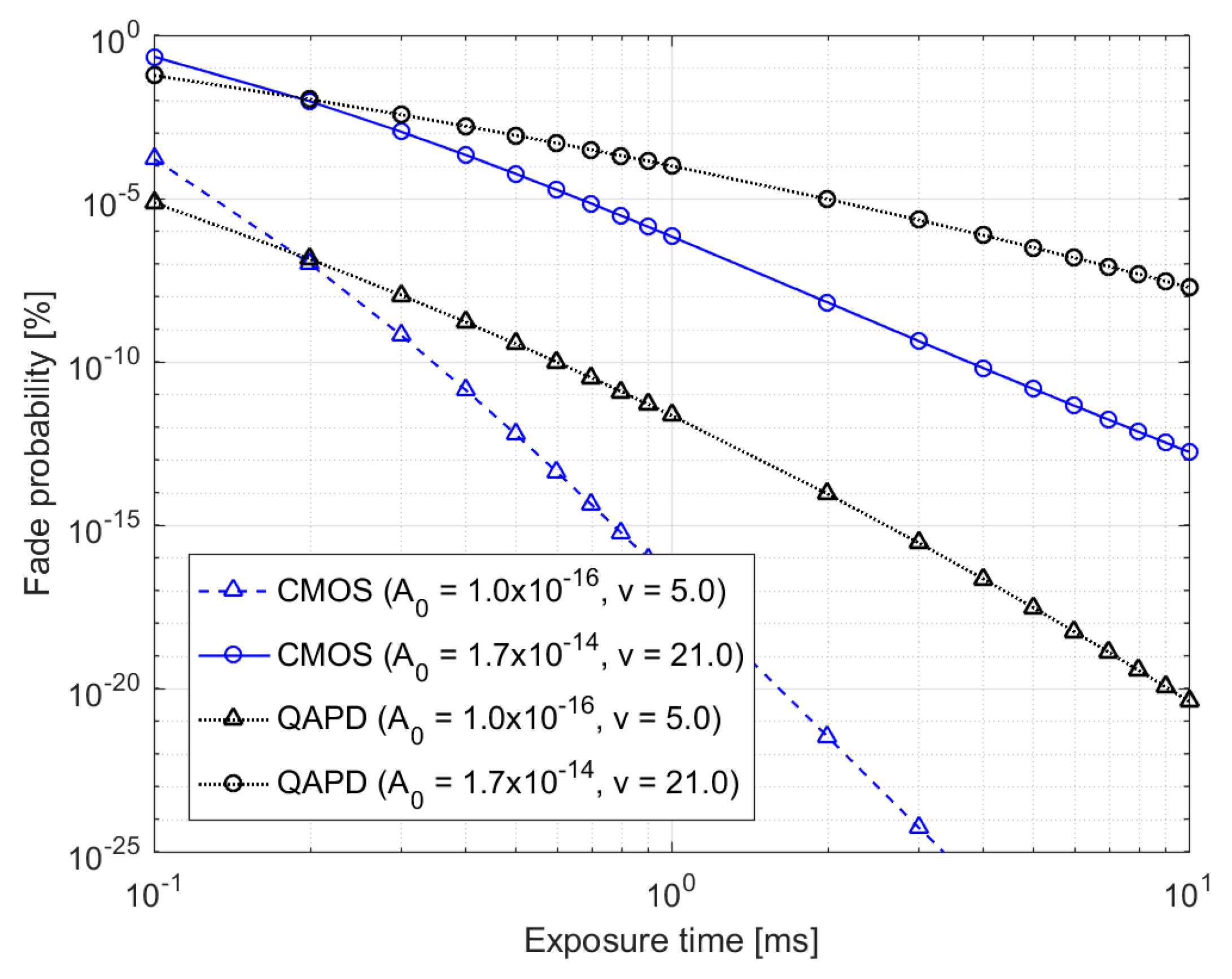
3.3. Fade Probability

Fade probability is a significant metric when evaluating the reliability of a tracking channel. It is defined as the probability when the SNR falls below a certain threshold over the tracking channels. It is related to the detector’s sensitivity limit, and can also be described in terms of received photon counts. Thus, the fade probability of a CMOS detector, over the log-normal tracking channels, is expressed as
P f C M O S = P ( γ C M O S γ t h C M O S ) = P ( K s K t h C M O S ) = 0 K t h C M O S f ( K s ) d K s = 1 2 e r f c ( ( ln K t h C M O S m k ) 2 σ k )
where γ t h C M O S and K t h C M O S are the thresholds in terms of SNR and received photoelectron counts, respectively, and e r f c ( ) is the complementary error function.
Applying the same conditions as Equation (24), the fade probability of a QAPD detector is also expressed as
P f Q A P D = 0 K t h Q A P D f ( K s ) d K s = 1 2 e r f c ( ( ln K t h Q A P D m k ) 2 σ k ) ,
where K t h Q A P D is the threshold of received photoelectron counts. Given that the SNR threshold is 1 (i.e., γ t h C M O S = 1 and γ t h Q A P D = 1 ), we can compute two thresholds for the CMOS and QAPD detectors from Equations (13) and (15): K t h C M O S = ( 1 + 1 + 4 K n C ) / 2 and K t h Q A P D = ( F + F 2 + 4 K n Q ) / 2 .

4. Numerical Results

In this section, we present the numerical results of an analysis of the angular positioning performance of two beacon detectors (CMOS and QAPD) over log-normal tracking channels in terms of centroid error and fade probability. The numerical simulation was performed by considering two detectors onboard a small satellite placed at an altitude ( H + h s ) of 500 km and a zenith angle θ z of 70°, leading to a distance z of 1193 km from an optical ground station located at a height h s of 100 m. The station transmits a beacon laser to the satellite with a wavelength λ of 850 nm, the transmitting power P T of 10 W [19,43], the transmitting optical efficiency η T of 0.95, the divergence θ D of 2.5 mrad in half-angle, and the pointing error θ e of 1.5 mrad, leading to a received power loss of 3 dB. Taking a clear sky into account, the atmospheric attenuation coefficient and cirrus cloud thickness were σ ( λ , V , 0 ) = 0.25 and C T = 1100 m , respectively. The spectral radiance of the background is assumed to be L λ = 71 W / m 2 ster μ m at 850 nm.
To compare the angular positioning performance of the two detectors in the presence of atmospheric turbulence, the two detectors were considered to have the same optical configurations including receiving aperture and optical efficiency, so that the number of received photons on the detectors were of the same order. We selected the MT9P031 model as the CMOS detector [43], and the S4402-SPL model as the QAPD detector [44]. Considering the optical communication terminal onboard a CubeSat, the common parameters related to the receiver are summarized in Table 1.
Taking the beam spreading due to atmospheric turbulence into account, the average count of received photoelectrons can be calculated from the link equation, which is dominated by the detector exposure time. It is remarkable that the turbulence-induced beam spreading angle is so small (i.e., on the order of micro radians) that it is negligible compared to the beam divergence of 5 mrad in this simulation, but it has a great effect on the link equation for beam divergence with the order of micro radians.
Figure 2 shows the received photoelectron counts and SNRs under atmospheric turbulence with A 0 = 1.7 × 10 14 m 2 / 3 and v = 21 m / s in terms of the exposure time. The pixel number N p used for the centroid window was assumed to be 9. As expected from Equation (8), K s is proportional to the exposure time, and the K s of the QAPD detector is larger than that of the CMOS detector due to the high quantum efficiency. However, the SNR of the QAPD detector was higher than that of the CMOS detector in the short exposure time regime, and vice versa in the long exposure time regime. The results come from the fact that the noise counts (i.e., background, dark current, and thermal noises) are significantly dominated by the exposure time for the QAPD detector, while the readout noise is independent of the exposure time for the CMOS detector excluding background and dark current noises.
Given the optical configuration, the centroid error is influenced by not only noise sources, but also the finite delay time causing the temporal evolution of atmospheric turbulence. Note that the exposure time latency that causes the finite delay time is taken into consideration in this simulation. Figure 3 shows the average centroid errors due to noise sources over log-normal tracking channels, and Figure 4 shows the centroid errors due to the exposure time latency, for two atmospheric turbulence conditions (i.e., A 0 = 1.0 × 10 16 m 2 / 3 and v = 5 m / s for the weak turbulence condition, A 0 = 1.7 × 10 14 m 2 / 3 and v = 21 m / s for the moderate turbulence condition). Applying the average wind speed v ¯ of 15 m / s , these two turbulence conditions provide values of the scintillation index, coherence length, and time (i.e., σ s i 2 = 0.28 , r 0 = 14.1 cm and t 0 = 2.9 ms for the weak turbulence condition, and σ s i 2 = 0.79 , r 0 = 7.4 cm and t 0 = 1.6 ms for the moderate turbulence condition).
The average centroid error over log-normal tracking channels was obviously smaller under the weak turbulence condition than the moderate condition. Compared to the CMOS detector, in terms of the average centroid error, the QAPD detector showed better performance regardless of the exposure time, even though its SNR was lower than the CMOS detector in the long exposure time regime, as shown in Figure 2.
As shown in Equation (20), the centroid error resulting from the exposure time latency is totally unrelated to the detector types, but depends on exposure time, coherence length, and diffraction-limited optics ( λ / D ). The centroid error resulting from the exposure time latency increases significantly as the exposure time is extended, and atmospheric turbulence becomes stronger because the coherence length is inversely proportional to the strength of atmospheric turbulence.
The total centroid errors are shown in Figure 5 and Figure 6 for weak and moderate atmospheric turbulence conditions, respectively. The average centroid error due to noise sources was inversely proportional to exposure time, but the centroid error resulting from exposure time latency increased exponentially in accordance with exposure time. Consequently, an optimal exposure time exists, which produces the total smallest centroid error under the designed optical configuration and atmospheric turbulence. This optimal exposure time is one of the critical design factors considered to meet the pointing requirements of the beacon tracking system.
Under weak turbulence conditions, the total centroid accuracy was 1.8 μrad at an exposure time of 0.5 ms for the CMOS detector, and 1.2 μrad at the exposure time of 0.3 ms for the QAPD detector. In moderate turbulence conditions, the total centroid accuracy was 2.7 μrad at the exposure time of 0.4 ms for the CMOS detector, and 1.8 μrad at the exposure time of 0.2 ms for the QAPD detector. The QAPD detector provided better performance than the CMOS detector under atmospheric turbulence in terms of the total centroid accuracy, especially in the short exposure time domain. This means that the QAPD detector is more suitable for the PAT system, which requires accurate pointing capabilities and higher bandwidth for closed-loop beacon tracking.
The fade probabilities for the two turbulence conditions are shown in Figure 7, defined as the probability when the SNR falls below 1 over log-normal tracking channels due to the intensity fluctuations produced by atmospheric scintillation. In other words, they mean probabilities when the received photoelectron counts are less than the threshold values of K t h C M O S and K t h Q A P D for the CMOS and QAPD detectors, respectively. These threshold values increase as the exposure time becomes longer, since noise count is proportional to exposure time. The threshold values for fade probabilities were K t h C M O S = 65.6 and K t h Q A P D = 226.4 at the exposure time of 0.1 ms, and K t h C M O S = 141.8 and K t h Q A P D = 2262.2 at the exposure time of 10 ms, respectively. The big difference between the threshold values of two detectors at the exposure time of 10 ms occurred because the noise sources of the QAPD detector were dominated more by the exposure time than the CMOS detector. This means that the CMOS detector will provide a better performance than the QAPD detector at long exposure times, in terms of fade probability. As the exposure time increases, the fade probability decreases, since the increase in received photoelectron counts is higher than the threshold value increment, which has to be taken into consideration in the design of the beacon tracking system.

5. Conclusions

An accurate centroid estimation of beacon images is required to ensure a beacon tracking system will precisely point an optical beam toward a partner terminal, and provide a reliable optical communication link even in the presence of atmospheric turbulence. However, centroid accuracy is limited by finite delay time as well as noise sources including detector and background noises. Centroid error is also influenced by intensity fluctuations resulting from atmospheric turbulence, which can terminate the beacon tracking link.
In this study, we analyzed the performance of two beacon tracking detectors onboard small satellites under atmospheric turbulence in terms of two metrics: centroid error and fade probability. Taking into account the log-normal tracking channels, the closed-form expressions were derived for not only the average centroid error, but also fade probability. We investigated two metrics for CMOS and QAPD detectors through numerical simulations by considering the windowed readout mode of the CMOS detector for high bandwidth, and confining finite delay time to the exposure time latency. As the exposure time became longer, the average centroid error due to noise sources decreased, but the centroid error caused by exposure time latency increased exponentially.
Atmospheric turbulence degrades the performance of the beacon tracking system, which is a crucial factor in causing the large centroid error in the regimes of long exposure time rather than a short one (i.e., >1 ms) due to the angle of arrival fluctuations. In addition, it makes a big difference in fade probabilities between weak and moderate turbulence conditions, on 3 or 4 orders at the exposure time of 0.1 ms, and the longer the exposure time, the greater the difference.
An optimal exposure time exists that produces the smallest total centroid error in the presence of atmospheric turbulence. It ranges from 0.2 ms to 0.5 ms, depending on the detector type and the strength of atmospheric turbulence, and where the total centroid error is to the order of micro radians. The QAPD detector showed better performance for total centroid error than the CMOS detector, while the CMOS detector provided superior performance in terms of the fade probability. Thus, two metrics have to be taken into account in the PAT system design to improve beacon tracking accuracy and to ensure reliable beacon tracking link.

Author Contributions

Conceptualization, H.-C.L.; Formal analysis, H.-C.L. and C.-S.C.; Software, K.-P.S.; Writing—Original draft, H.-C.L.; Writing—Review & editing, C.-S.C. and J.-U.P.; Project administration, M.C. All authors have read and agreed to the published version of the manuscript.

Funding

This research received no external funding.

Institutional Review Board Statement

Not applicable.

Informed Consent Statement

Not applicable.

Data Availability Statement

All data generated or analyzed during this study are included in this article.

Acknowledgments

This work was supported by the Korea Astronomy and Space Science Institute through the project “Operation of Observation Facilities for Space Object Surveillance” funded by the Ministry of Science and ICT (MSIT) of the Korean government.

Conflicts of Interest

The authors declare no conflict of interest.

References

  1. Toyoshima, M.; Leeb, W.R.; Kunimori, H. Comparison of microwave and light wave communication systems in space application. Opt. Eng. 2005, 46, 1–12. [Google Scholar]
  2. Li, X.; Yu, S.; Ma, J. Analytical expression and optimization of spatial acquisition for intersatellite optical communications. Opt. Exp. 2011, 19, 2381–2390. [Google Scholar] [CrossRef]
  3. Ma, J.; Li, K.; Tan, L.; Yu, S.; Cao, Y. Performance analysis of satellite-to-ground downlink coherent optical communications with spatial diversity over Gamma- Gamma atmospheric turbulence. Appl. Opt. 2015, 54, 7575–7585. [Google Scholar] [CrossRef]
  4. Kaushal, H.; Kaddoum, G. Optical communication in space: Challenges and mitigation techniques. IEEE Commun. Surv. Tutor. 2016, 19, 57–96. [Google Scholar] [CrossRef] [Green Version]
  5. Lim, H.-C.; Park, J.U.; Choi, M.; Choi, C.-S.; Choi, J.-D.; Kim, J. Performance analysis of DPSK optical communication for LEO-to-Ground Relay link via a GEO Satellite. J. Astron. Space Sci. 2020, 37, 11–18. [Google Scholar]
  6. Meynants, G.; Lepage, G.; Bogaerts, J.; Vanhorebeek, G.; Wang, X. Limitations to the frame rate of high speed image sensors. In Proceedings of the 2009 International Image Sensor Workshop, Bergen, Norway, 22–28 June 2009. [Google Scholar]
  7. Cierny, O. Precision Closed-Loop Laser Pointing System for the Nanosatellite Optical Downlink Experiment. Master’s Thesis, Lulea University of Technology, Lulea, Sweden, 2017. [Google Scholar]
  8. Anugu, N.; Amorim, A.; Gordo, P.; Eisenhauer, F.; Pfuhl, O.; Haug, M.; Wieprecht, E.; Wiezorrek, E.; Lima, J.; Perrin, G.; et al. Methods for multiple-telescope beam imaging and guiding in the near-infrared. MNRAS 2018, 476, 459–468. [Google Scholar] [CrossRef] [Green Version]
  9. Ivan, I.A.; Ardeleanu, M.; Laurent, G.J. High dynamics and precision optical measurement using a position sensitive Detector (PSD) in reflection-mode: Application to 2D object tracking over a smart surface. Sensors 2012, 12, 16771–16784. [Google Scholar] [CrossRef] [PubMed]
  10. Toyoshima, M. Trends in satellite communications and the role of optical free-space communications. J. Opt. Netw. 2005, 4, 300–311. [Google Scholar] [CrossRef]
  11. Buske, I.; Riede, W. Sub-μrad laser beam tracking. In Technologies for Optical Countermeasures III, Proceedings of the Optics/Photonics in Security and Defence, Stockholm, Sweden, 11–14 September 2016; SPIE: Cardiff, Wales, UK, 2006. [Google Scholar]
  12. Hemmati, H. Near-Earth Laser Communications; CRC Press: Boca Raton, FL, USA, 2009. [Google Scholar]
  13. Leeb, W. Space laser communications: Systems, technologies, and applications. Rev. Laser Eng. 2000, 28, 804–808. [Google Scholar] [CrossRef] [Green Version]
  14. Kaminow, I.P.; Li, T.; Willner, A.E. Optical Fiber Telecommunications VIB; Elsevier Inc.: Waltham, MA, USA, 2013. [Google Scholar]
  15. Carrasco-Casado, A.; Biswas, A.; Fields, R.; Grefenstette, B.; Harrison, F.; Sburlan, S.; Toyoshima, M. Optical communication on CubeSats—Enabling the next era in space science. In Proceedings of the 2017 IEEE International Conference on Space Optical Systems and Applications (ICSOS), Okinawa, Japan, 14–16 November 2017. [Google Scholar]
  16. Dios, F.; Rubio, J.A.; Rodriguez, A.; Comeron, A. Scintillation and beam-wander analysis in an optical ground station-satellite uplink. Appl. Opt. 2004, 43, 3866–3873. [Google Scholar] [CrossRef] [PubMed] [Green Version]
  17. Cui, A. Analysis of angle of arrival fluctuations for optical wave’s propagation through weak anisotropic non-Kolmogorov turbulence. Opt. Exp. 2015, 23, 6313–6325. [Google Scholar] [CrossRef] [PubMed]
  18. Lim, H.-C.; Zhang, Z.-P.; Sung, K.-P.; Park, J.U.; Kim, S.; Choi, C.-S.; Choi, M. Modeling and analysis of an echo laser pulse waveform for the orientation determination of space debris. Remote Sens. 2020, 12, 1659. [Google Scholar] [CrossRef]
  19. Nguyen, T.N. Laser Beacon Tracking for Free-space Optical Communication on Small-Satellite Platforms in Low-Earth Orbit. Master’s Thesis, Massachusetts Institute of Technology, Cambridge, MA, USA, 2013. [Google Scholar]
  20. Tyler, G.A.; Fried, D.L. Image-position error associated with a quadrant detector. J. Opt. Soc. Am. 1982, 72, 804–808. [Google Scholar] [CrossRef]
  21. Lee, S. Pointing accuracy improvement using model-based noise reduction method. In Free-Space Laser Communication Technologies XIV, Proceedings of the High-Power Lasers and Applications, San Jose, CA, USA, 20–25 January 2002; SPIE: Cardiff, Wales, UK, 2002. [Google Scholar]
  22. Hemmati, H. Deep Space Optical Communications; Jet Propulsion Laboratory: Pasadena, CA, USA, 2005. [Google Scholar]
  23. Sandler, D.G.; Stahl, S.; Angel, J.R.P.; Lloyd-Hart, M.; McCarthy, D. Adaptive optics for diffraction-limited infrared imaging with 8-m telescopes. J. Opt. Soc. Am. A 1994, 11, 925–945. [Google Scholar] [CrossRef]
  24. Colucci, D.; Lloyd-Hart, M.; Wittman, D.; Angel, R.; Ghez, A.; Mcleod, B. A reflective shack-hartmann wave-front sensor for adaptive optics. Publ. Astron. Soc. Pac. 1994, 106, 1104–1110. [Google Scholar] [CrossRef]
  25. Thomas, S.; Fusco, T.; Tokovinin, A.; Nicolle, M.; Michau, V.; Rousset, G. Comparison of centroid computation algorithms in a Shack-Hartmann sensor. Mon. Not. R. Astron. Soc. 2006, 371, 323–336. [Google Scholar] [CrossRef] [Green Version]
  26. Nightingale, A.M.; Gordeyev, S. Shack-Hartmann wavefront sensor image analysis: A comparison of centroiding methods and image-processing techniques. Opt. Eng. 2013, 52, 071413. [Google Scholar] [CrossRef]
  27. Li, C.; Xian, H.; Rao, C.; Jiang, W. Measuring statistical error of Shack–Hartmann wavefront sensor with discrete detector arrays. J. Mod. Opt. 2008, 55, 2243–2255. [Google Scholar] [CrossRef]
  28. Tsiftsis, T.A.; Sandalidis, H.G.; Karagiannidis, G.K.; Uysal, M. Optical wireless links with spatial diversity over strong atmospheric turbulence channels. IEEE Trans. Wirel. Commun. 2009, 8, 951–957. [Google Scholar] [CrossRef] [Green Version]
  29. Mishra, N.; Kumar, D.S. Outage analysis of relay assisted FSO systems over K-distribution turbulence channel. In Proceedings of the 2016 International Conference on Electrical, Electronics, and Optimization Techniques (ICEEOT), Chennei, India, 3–5 March 2016; pp. 2965–2967. [Google Scholar]
  30. Al-Habash, M.A.; Andrews, L.C.; Phillips, R.L. Mathematical model for the irradiance probability density function of a laser beam propagating through turbulent media. Opt. Eng. 2001, 40, 1554–1562. [Google Scholar] [CrossRef]
  31. Kiasaleh, K. Performance of APD-based, PPM free-space optical communication systems in atmospheric turbulence. IEEE Trans. Commun. 2005, 53, 1455–1461. [Google Scholar] [CrossRef]
  32. Andrews, L.C.; Phillips, R.L. Laser Beam Propagation through Random Media; SPIE Press: Bellingham, WA, USA, 2005. [Google Scholar]
  33. Nistazakis, H.E.; Tsiftsis, T.A.; Tombras, G.S. Performance analysis of free-space optical communication systems over atmospheric turbulence channels. IET Commun. 2009, 3, 1402–1409. [Google Scholar] [CrossRef]
  34. Johnson, S.E. Effect of target surface orientation on the range precision of laser detection and ranging systems. J. Appl. Remote Sens. 2009, 3, 033564. [Google Scholar] [CrossRef]
  35. Degnan, J.J. Milimeter accuracy satellite laser ranging: A review. Geodyn. Ser. 1993, 25, 133–162. [Google Scholar]
  36. Shen, H.; Yu, L.; Fan, C. Temporal spectrum of atmospheric scintillation and the effects of aperture averaging and time averaging. Opt. Commun. 2014, 330, 160–164. [Google Scholar] [CrossRef]
  37. Ghassemlooy, Z.; Popoola, W.; Rajbhandari, S. Optical Wireless Communications: System and Channel Modelling with MATLAB.; CRC Press: Boca Raton, FL, USA, 2018. [Google Scholar]
  38. Gunderson, K.; Thomas, N.; Rohner, M. A Laser altimeter performance model and its application to BELA. IEEE Trans. Geosci. Remote Sens. 2006, 44, 3308–3319. [Google Scholar] [CrossRef]
  39. Ma, X.; Rao, C.; Zheng, H. Error analysis of CCD-based point source centroid computation under the background light. Opt. Exp. 2009, 17, 8525–8541. [Google Scholar] [CrossRef]
  40. Barry, J.D.; Mecherle, G.S. Beam pointing error as a significant design parameter for satellite-borne, free-space optical communication systems. Opt. Eng. 1985, 24, 1049–1054. [Google Scholar] [CrossRef]
  41. Tyler, G.A. Bandwidth considerations for tracking through turbulence. J. Opt. Soc. Am. A 1994, 11, 358–367. [Google Scholar] [CrossRef]
  42. Roddier, R. The effects of atmospheric turbulence in optical astronomy. Prog. Opt. 1981, 19, 281–376. [Google Scholar]
  43. Riesing, K.M. Development of a Pointing, Acquisition, and Tracking System for a Nanosatellite Laser Communication Module. Master’s Thesis, Massachusetts Institute of Technology, Cambridge, MA, USA, 2013. [Google Scholar]
  44. Toyoda, M.; Araki, K.; Suzuki, Y. Measurement of the characteristics of a quadrant avalanche photodiode and its application to a laser tracking system. Opt. Eng. 2002, 41, 145–149. [Google Scholar] [CrossRef]
Figure 1. Block diagram of the optical communication terminal with monostatic architecture.
Remotesensing 13 01931 g001
Figure 2. Received photoelectron counts and SNRs versus the exposure time under atmospheric turbulence with A 0 = 1.7 × 10 14 m 2 / 3 and v = 21 m / s .
Remotesensing 13 01931 g002
Figure 3. Average centroid error due to noise sources versus exposure time under two atmospheric turbulence conditions.
Remotesensing 13 01931 g003
Figure 4. Centroid error due to delay time (i.e., exposure time in the simulation) versus exposure time under two atmospheric turbulence conditions.
Remotesensing 13 01931 g004
Figure 5. Total centroid error under weak atmospheric turbulence conditions.
Remotesensing 13 01931 g005
Figure 6. Total centroid error under moderate atmospheric turbulence conditions.
Remotesensing 13 01931 g006
Figure 7. Fade probability versus exposure time under two atmospheric turbulence conditions.
Remotesensing 13 01931 g007
Table 1. Receiver parameters used in the numerical simulation.
ParameterSymbolCMOSQAPD
Rx aperture D 2.5 cm
Rx optical efficiency η R 0.68
Optical filter bandwidth Δ λ f i l t e r 4 nm
Quantum efficiency η Q 0.150.7
Focal length 4.1 cm7.9 cm
Active pixels 2592 × 19444
Active area 5.7 × 4.28 mm21.77 mm2
Pixel size 2.2 × 2.2 μm20.44 mm2
Publisher’s Note: MDPI stays neutral with regard to jurisdictional claims in published maps and institutional affiliations.

