The Application of an Unmanned Aerial System and Machine Learning Techniques for Red Clover-Grass Mixture Yield Estimation under Variety Performance Trials

Abstract

A significant trend has developed with the recent growing interest in the estimation of aboveground biomass of vegetation in legume-supported systems in perennial or semi-natural grasslands to meet the demands of sustainable and precise agriculture. Unmanned aerial systems (UAS) are a powerful tool when it comes to supporting farm-scale phenotyping trials. In this study, we explored the variation of the red clover-grass mixture dry matter (DM) yields between temporal periods (one- and two-year cultivated), farming operations [soil tillage methods (STM), cultivation methods (CM), manure application (MA)] using three machine learning (ML) techniques [random forest regression (RFR), support vector regression (SVR), and artificial neural network (ANN)] and six multispectral vegetation indices (VIs) to predict DM yields. The ML evaluation results showed the best performance for ANN in the 11-day before harvest category (R² = 0.90, NRMSE = 0.12), followed by RFR (R² = 0.90 NRMSE = 0.15), and SVR (R² = 0.86, NRMSE = 0.16), which was furthermore supported by the leave-one-out cross-validation pre-analysis. In terms of VI performance, green normalized difference vegetation index (GNDVI), green difference vegetation index (GDVI), as well as modified simple ratio (MSR) performed better as predictors in ANN and RFR. However, the prediction ability of models was being influenced by farming operations. The stratified sampling, based on STM, had a better model performance than CM and MA. It is proposed that drone data collection was suggested to be optimum in this study, closer to the harvest date, but not later than the ageing stage.

1. Introduction

Red clover (Trifolium pratense L.) is the principal perennial forage crop legume species in most countries of northern Europe, including Estonia [1,2]. Legumes have the ability to increase the productivity of grass pastures by fixing atmospheric nitrogen into the soil; via the symbiotic rhizobia in their root nodules [3]. This fixation of atmospheric nitrogen makes red clover an ideal rotational crop; particularly in organic agricultural systems where no synthetic nitrogen fertilizers are used [4]. A range of studies have observed that the establishment of red clover was more successful when sown in mixtures with grass species rather than in pure, monocultural stands [5,6]. In Estonia, the application of red clover in trials results in a mixed-species approach with other grass species blended to increase its commercial application value, where the complexity of estimation might be higher than monocropping systems. Legume-based systems, and in particular red clover practices, are economically attractive to dairy farmers in northern Europe and are essential for ensuring that organic systems can compete in terms of profitability with more conventional or artificially improved systems [7]. The success of red clover in pasture farming systems makes it a vital economical crop regardless of whether it is integrated into conventional or organic farming operations. Besides their positive effects on farming productivity, legumes can also play a part in lowering greenhouse gas emissions by reducing the use of inorganic nitrogen fertilizers and replacing them with symbiotically fixed nitrogen, and the use of perennial grass species, a common practice, to reduce carbon loss in cultivated soil [8]. This approach improves the sustainability of the agricultural ecosystem compared to monocropping systems, as well as contributes to the conservation value for threatened bumblebee species [9]. In Estonia, the cultivation of clover-grass mixtures had played significant agronomic purposes in co-cultivation and increased the feed value of the mixture, sequestering nitrogen and thereby reducing the amount of fertilizer [10], and achieving C-balance and carbon sequestration [11] in crop rotation through perennial grassland.

However, it is important to note that with the present trend towards global trade, the increased importation of grain legumes into Europe has led to lower local production in many countries [12]. This trend has raised questions regarding the sustainability and security of protein supplies [13]. Perhaps in opposition to this, the main direction of red clover cultivation goals has focused on forage yields and persistence [14], which may directly improve business competitiveness and increase agricultural versatility. This also highlights the importance of the estimation and quantification of high-yield clover and grass mixtures, and in particular extending from the laboratory to field-based performance trials and studies. Traditional on-site destructive silage and forage biomass sampling and measurements provide accurate reference data for building and assessing yield models. However, it is time-consuming, highly labor-intensive, and limited by large-scale spatial quantity parameter collection [15]. Also, trials and phenotyping techniques have become increasingly criticized in recent years. One of the objectives of this study is to explore and expand the monitoring range from controlled environments, such as laboratories and greenhouses, to bare soil-based situations [16,17]. Variety performance trials (VPT), as an alternative, is a randomized controlled field-based experimental design to improve environment × management scenario recommendations for variety comparison and breeding selection [18,19]. A typical approach of VPT is recognizing multiple crop phenotypes and their response to management practices. With the current raised awareness of environmental protection and the concept of sustainable agriculture, the adaptability of eco-friendly cultivation techniques, such as reduced tillage and the application of various minerals and organic fertilizers are emerging [20]. However, the description of these managements in current VPT systems is indispensable for vigorous simulation and rigorously assessed for their ability to reproduce measured crop yields that established near-optimal management practices [21].

These limitations and challenges associated with silage and forage legumes have, to some degree, promoted and encouraged the development of remote sensing (RS) solutions for legume biomass estimation tasks [22]. The use of RS offers cost-efficient, non-destructive, and spatially extensive approaches for crop monitoring and trait decision-making. Equally, RS approaches can support yield prediction and help to determine and assess a multifaceted range of plant traits when combined with modeling of phenotypic features [23]. Its application in agriculture is also a vital tool in further understanding plant-environment interactions within the management of crops [24]. Therefore, it is necessary to broaden the horizon of rapid and accurate RS approaches in the analyses of red clover-grass mixture trials in response to multiple farming techniques and operations.

More recently, Unmanned Aerial Systems (UAS) offer significant potential to support and develop current and future red clover trial studies. It has arisen as a cost-efficient remote-sensing platform for capturing high-resolution imagery [25]. The recent expansion of sensors and cameras that can be integrated with, and mounted on, these systems offers the capability to distinguish and compare plant changes both spatially and temporally for the detection and differentiation of local agricultural practices [26]. For example, the reflectance of vegetation information captured by UAS-borne sensors is verified by biological and morphological features of the surface of tissues or leaves [27]. Depending upon the sensor types (e.g., visible spectrum or multispectral), the vegetation light spectra that can be captured can range from the ultraviolet region (UV), the visible region (RGB), through to near-infrared region (NIR). Furthermore, when captured across a series of these ranges, this information can be used to calculate several vegetation indices (VIs). VIs are widely utilized in the assessment of crop characteristics with the ability to reduce soil or environmental noise and enhance their sensitivity for a target characteristics [15]. One of the most applied multispectral VI is the Normalized Difference Vegetation Index (NDVI) with its ratio between the red and near-infrared bands [28]. However, NDVI is not only sensitive to soil and atmospheric effects, but also certain spectrum ranges were found to have an asymptotic relation, as applicability is limited for higher biomass levels [29,30]. Also, the ability of the reflectance sensor in biomass prediction could be limited by aging crop materials and diverse canopy structures caused by mixed species [15]. Therefore, an alternative for increasing the accuracy of various crop modeling tasks is by increasing the varieties and combinations of adjusted and optimized VIs [31].

Several UAS-based forage clover studies have been conducted in recent years. UAS-RGB-based vegetation indexes and linear regression models were utilized in estimating the red clover dry matter (DM) yield with the best performance R² values 0.62 [32]. UAS-RGB-based point cloud data generated into photogrammetric canopy height models (CHM) can also be utilized in forage legumes DM prediction; clover-grass canopies showed better performance than lucerne-grass mixtures for DM prediction [33]. Concerning another study combining CHM, RGB, and VIs with machine learning (ML) techniques for grass swards silage prediction, the Pearson correlation coefficients reached 0.98 [34]. Equally, clover-related phenotypic research has also received much attention in recent years: it included clover-grass pasture coverage and spatial dynamics monitoring [35,36], and quality parameters, such as the digestibility of organic matter, water-soluble carbohydrates, the nitrogen concentration, and uptake [37]. These studies largely used UAS-derived images combined with state-of-the-art ML technologies for qualitative or quantitative analysis. However, red clover silage and forage biomass studies require the establishment and characterization of multiple management options, such as fertilizers, tillage methods, and farming systems, in order to meet the actual planting condition and provide valuable feedback to local farmers and policymakers. There is little scrutiny on the application of DM modeling in the response to the above-mentioned factors.

A gap, therefore, currently exists in the knowledge base for legume biomass analysis and the further understanding of the potential for remotely-sensed solutions to field-based and multifunctional platforms for the demands of precision agriculture. To address this knowledge gap, this study presents a rapid, non-destructive, low-cost framework for field-based red-clover DM yield modeling. The outputs could potentially assist agronomists and farmers in developing precise farming systems and increase the effective monitoring of environmental conditions. More specifically, the objectives of this study are the comparison of two temporal pre-harvest (11 days and 38 days) DM prediction capabilities under one- and two-year clover-grass cultivation fields with three different treatments; and the comparison of the performance of three machine learning algorithms and their corresponding variable importance rankings in estimating clover-grass mixture DM. To address these aims, UAS-multispectral data and six VIs were extracted and used for training and evaluation models.

2. Materials and Methods

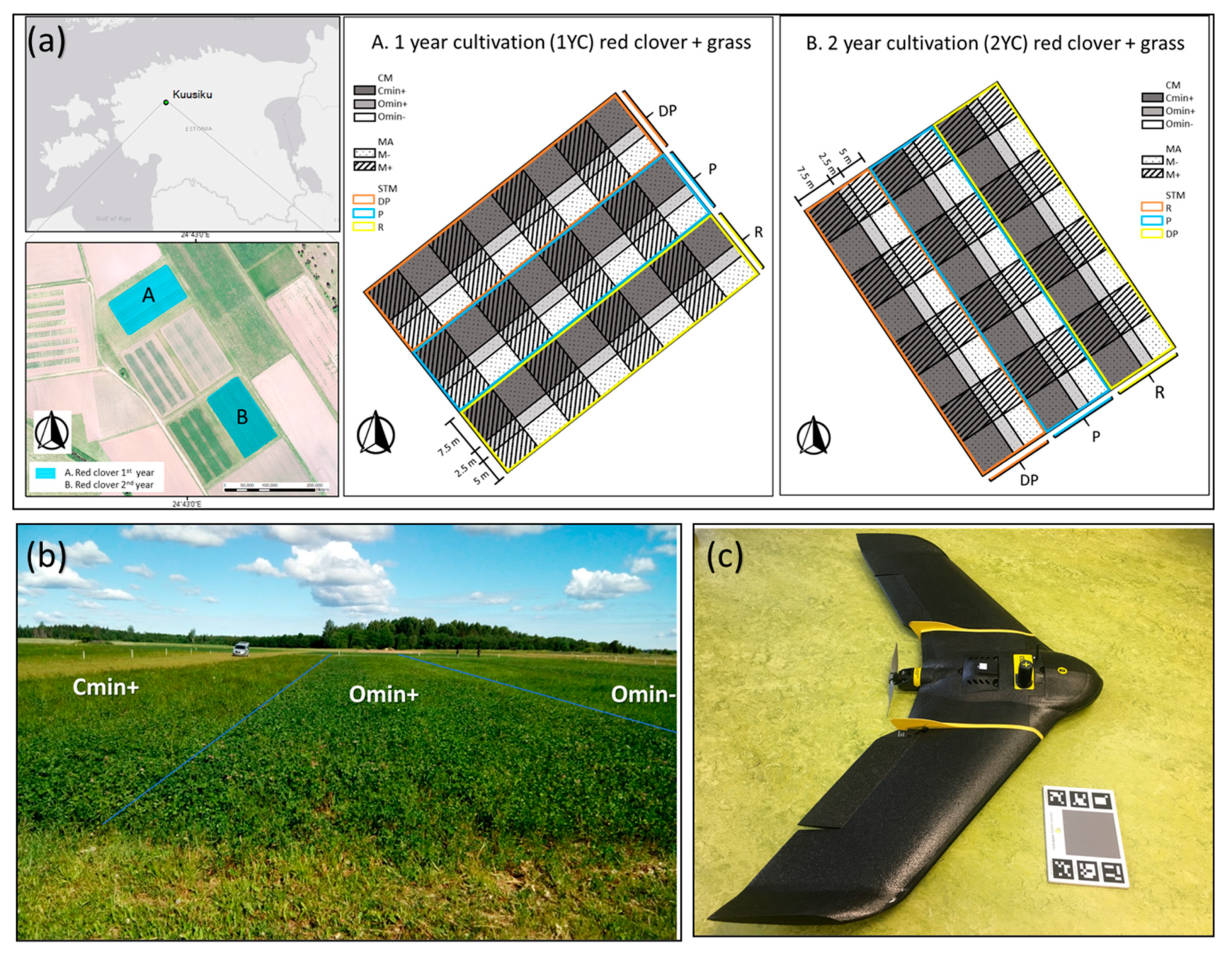
2.1. Study Area and Experiment Layout

This study was undertaken at the Agricultural Research Centre (ARC) in Kuusiku (58°58′52.7″N 24°42′59.1″E), Estonia (Figure 1a). The ARC was established in 1924 by an official institution under the governance of the Ministry of Agriculture and consists of consolidated laboratories and field testing centers. The experimental area covers 226 hectares, of which the variety performance trial area we selected to consist of two soil types: Calcaric Cambisol and Calcari-Leptic Regosol [38].

In this study, red clover was used in grass-mixture for the representation in practical farming purposes. More specifically, approximately 75% of the mixture consisted of red clover (Trifolium pratense L.) tetraploids variety ‘Varte’, an early variety normally cropped in Estonia, and the remaining 25% of the mix comprised of meadow fescue (Festuca pratensis)—variety ‘Jõgeva 47’. To assess the potential of UAS-based DM prediction capacity in the agricultural application of the clover-grass mixture field, the experiment was designed with three principal experimental factors (see

Table 1. The farming operation and treatment of the red clover experiment fields.

Farming Operation	Treatment	Description
Soil tillage methods (STM)	Reduced tillage (R)	R (8–10 cm)
	Ploughing (p)	P (18–20 cm)
	Disking and ploughing (DP)	D (8–10 cm) & P (18–20 cm)
Cultivation methods (CM)	Conventional framing with fertilizer (Cmin+)	NPK 5-10-25 1
	Organic farming with mineral fertilizer (Omin+)	Patentkali 2
	Organic farming without mineral fertilizer (Omin−)	N/A
Manure application (MA)	With manure application (M+)	M (30,000 kg ha−1) 3
	Without manure application (M−)	N/A

¹ NPK 5-10-25 (chemical fertilizer) 291 kg ha⁻¹ (N-14 kg ha⁻¹, P-13 kg ha⁻¹, and K-60 kg ha⁻¹); ² Patentkali (mineral fertilizer) 240 kg ha⁻¹ (K-60 kg ha⁻¹, S- 41 kg ha⁻¹, M-14 kg ha⁻¹); ³ Manure 30,000 kg ha-1 (N-234 kg ha⁻¹, P-20 kg ha⁻¹, and K-216 kg ha⁻¹).

). More specifically, these included: (1) soil tillage methods (STM), considering reduced tillage (R) (8–10 cm), ploughing (P) at a depth traditionally used in conventional tillage (18–20 cm), and disking (DP) (8–10 cm) as treatments; (2) cultivation methods (CM) (as shown in Figure 1b), considering conventional farming with mineral fertilizer application (CMin+), organic farming with mineral fertilizer application (OMin+), and organic farming without mineral fertilizer (OMin-); and (3) manure applications (MA). Considering the convenience of ploughing and fertilizer applications, we present the design of the field and location as shown in Figure 1a, and the treatment details in Table 1. The mixture’s fresh aboveground biomass was cut twice in two fields (1YC and 2YC). Each field contains 72 plots, which means a total of 144 plots were sampled; the first cut took place on 10/06/2019, and the second took place on 16/08/2019. The fresh biomass was weighed by plot and dried to verify its DM yield measured in kilograms per hectare.

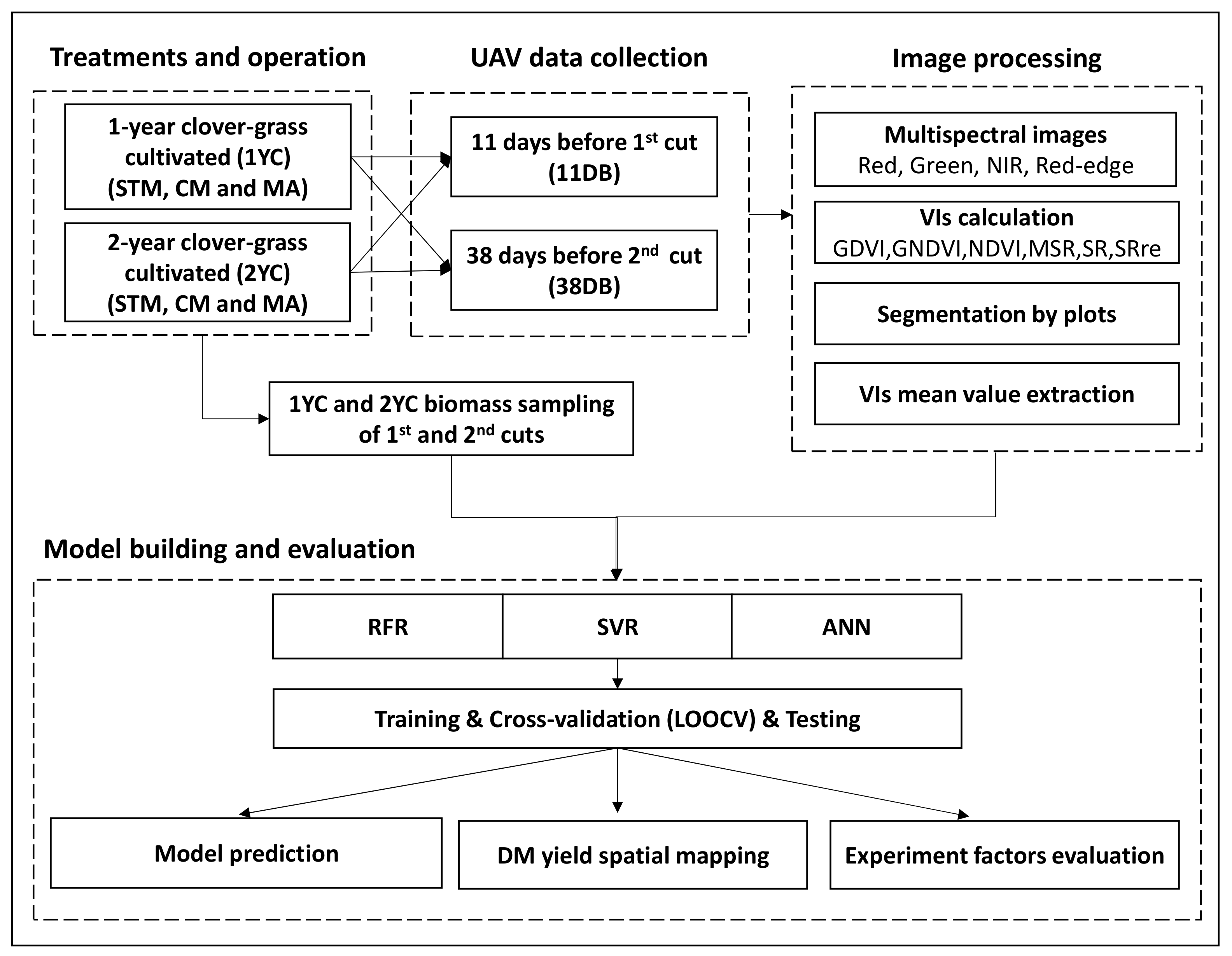
2.2. Image Acquisition

Figure 2 presents a workflow of the methodology used to combine the UAS-based image collection, processing, biomass sampling, as well as modeling and evaluation within ML algorithms. To capture data for both image processing and biomass evaluations, the UAS imaging was conducted twice [i.e., 11 days before 1st cut (11DB) and 38 days before 2nd cut (38DB) harvesting] in the summer of 2019. Due to the needs of the other experimental areas, the data of 80 hectares were collected, of which 2.4 hectares were used in this study. An eBee Plus device (Figure 1c), with onboard GNSS post-processed kinematic (PPK) capabilities, was deployed and equipped with a Parrot Sequoia multispectral sensor. The Parrot Sequoia sensor captured imagery across four spectral bands: near-infrared (770–810 nm); red-edge (730–740 nm); red (640–680 nm); and green (530–570 nm). The flight lines overlap was set with a frontal image overlap of 80% and lateral image overlap of 75%. All the operations took place between 10 a.m. to 2 p.m. to ensure consistency with the sun’s angle, and to reduce lateral shading within the experimental fields. The images were captured from a height of 120 meters, and the resulting images had ground sampling distance (GSD) of 10 cm per pixel. Prior to each flight mission, an Airinov radiometric calibration target and one-point calibration method [39] was used to facilitate post-flight radiometric correction of the multispectral imagery.

Table 2. Specification of the weather condition and the corresponding time before harvest.

Date of Flight	Weather	Wind Speed (km/h)	Wind Direction	Temperature (min-max°C)	Humidity	Operation
30 May 2019	Sunny	11	S	15–16	35%	11 days before 1st cut (11DB)
1 July 2019	Overcast	12	WSW	19–20	64%	38 days before 2nd cut (38DB)

provides a summary of environmental conditions for the two flights conducted prior to clover-grass biomass harvesting.

2.3. Image Processing and Analysis

The UAS data was post-processed in SenseFly eMotion 3 [40] using receiver independent exchange (RINEX) format data provided by the GNSS CORS (Continuously Operating Reference Station) of Estonia [41] for post-processing kinematics (PPK) corrections. This post-process provided an increase in the geotagging accuracy [42] of the UAS images from 5 m error to under 0.06 m, where the method and accuracy obtained is similar to [43]; and thus less than the one-pixel size in our study. Pix4D v.4.3.31^® (Pix4D SA, 1015 Lausanne, Switzerland) software was utilized to process and radiometrically correct (default in Pix4D) the imagery and generate the multispectral orthomosaics. These images were subsequently clipped to represent only the extent of the experimental area.

2.4. Vegetation Indices Calculation and Extraction

In this study, six VIs were calculated using R version 4.0.2 [44] (

Table 3. Descriptions and formulas of NIR-related VIs used in this study.

Vegetation Index	Description	Equation	Reference
NDVI	Normalized Difference Vegetation Index	(ρ NIR − ρ R 1)/(ρ NIR + ρ R)	[28]
GNDVI	Green Normalized Difference Vegetation Index	(ρ NIR − ρ G 2)/(ρ NIR + ρ G)	[52]
GDVI	Green Difference Vegetation Index	ρ NIR 3 − ρ G	[53]
SR	Simple Ratio	ρ NIR/ρ R	[54]
SRre	Red-edge simple ratio	ρ NIR/ρ REG 4	[55]
MSR	Modified simple ratio	((ρ NIR − ρ R) − 1)/(((ρ NIR + ρ R) ∗ (0.5)) + 1)	[51]

¹ ρ R refers to red band, ² ρ G refers to green band, ³ ρ NIR refers to near-infrared, and ⁴ ρ REG refers to the red edge.

). The normalized difference vegetation index (NDVI) utilizes the reflectance (ρ) in the NIR and Red wavelengths, and the outputs range from −1.0 to 1.0. This index was selected for this study as it has a sensitive response to track physiological dynamics and biomass [45]. However, NDVI reaches saturation when leaf area index (LAI) values are about 2.5–3 or in dense crop canopies [46,47]. The green normalized difference vegetation index (GNDVI) was also calculated and outputs values range from 0 to 1. Previous studies have shown GNDVI to be linearly correlated with LAI and biomass, with the ability to reduce the effects of soil reflectance and estimate nitrogen conditions [48]. Similarly, the Simple Ratio (SR), a normalization of ρ NIR against ρ Red, was calculated as it has been previously shown that this index can better indicate the strength of canopy photosynthetic material and yield prediction better than NDVI under different nitrogen supplies [49]. The Red-Edge Simple Ratio (SRre) formula was calculated by replacing the ρ Red band with the ρ Red-edge. Its inclusion in the assessment was due to previous studies indicating a higher correlation with plant nitrogen concentration compared to ρ Red based VIs. This can lessen the soil background influence on crop reflectance [50]. Finally, the Modified Simple Ratio (MSR), as a potentially improved version of the Renormalized Difference Vegetation Index (RDVI), was calculated to linearize the relationship between biophysical parameters [51] and enhance the sensitivity of vegetation occurrences, which can be observed in other VIs.

The two experimental fields [i.e., 1YC (n = 72) and 2YC (n = 72)], with a total of 144 plots were digitized in ArcGIS Pro 2.6.3 [56]. The average VIs within each plot were extracted and calculated as the VIs of each plot at the experiment site. To avoid potential edge effects in the fertilizer treatment, a one-meter buffer zone was extended inwards from each plot boundary, and data sampled within this target region (Figure 3). These extracted values were further used in this study when building ML algorithms for clover-grass mixture DM yield estimation and evaluation.

2.5. Machine Learning Techniques

Parametric regression models may lead to multicollinearity between covariates and overfitting, which renders them impractical when dealing with highly dimensional remotely sensed data [57]. Conversely, machine learning algorithms can handle high volumes of predictor variables that are interrelated and have a non-linear relationship with response variables [58]. A recent remote sensing-based ML study collected data from 220 related articles and found that random forest (RF), support vector machine (SVM), and artificial neural network (ANN) algorithms were amongst the most used ML techniques [59]. Therefore, these derived ML regressions [random forest regression (RFR), support vector regression (SVR), and artificial neural network (ANN)] were chosen for modeling DM in this study. These algorithms were programmed in Python [60] (version 3.8). The VI values presented in Table 3 were used as continuous predictor variables of the DM regression models, which were divided into training sites and prediction sites, and the parameters of each algorithm were adapted to ensure the performance as effectively as possible for our training and testing dataset.

First, to reduce the potential over-fitting problem of the model, a leave-one-out cross-validation (LOOCV) procedure [61] was conducted to validate the three ML techniques. The LOOCV procedure involves creating a model by separating one sample for testing and the rest (n = 36) for validation in every iteration. (Figure 4a). Second, all training sites were used to model and predict the three ML methods (Figure 4b). As the training and testing dataset comprised two repetitions of results from each treatment, a comprehensive range of crop conditions were covered by the modeling. The variable importance of the VIs was calculated for each ML technique differently and was listed per each model’s VIs importance scores, and the suitable models for different periods for DM yield spatial mapping were demonstrated. Finally, experimental treatments (i.e., STM, CM, and MA) were used to explore the relationship between different experiment factors and models (Figure 4d). The testing sites were sampled following a stratified approach based on the three different farming operations, 3 strata with 12 samples in each one in STM (DP, P, and R) and CM (Cmin, Omin+, and Omin−) groups, and 2 strata with 18 samples in MA (M+, and M−). The ML methods, selected parameters, model evaluation techniques, and variable importance calculations are described below.

2.5.1. Random Forest Regression

An adaptation of the Random Forest (RF) algorithm [62] was conducted for DM regression models (i.e., RFR). The RFR algorithm fits an ensemble of decision tree models to a set of data. The regression tree algorithm creates individual decision trees automatically based on randomly chosen samples and subsets of the training data. For random forest construction, the best split is selected among a random subset of the predictors at each node. Calculations were conducted with 100 trees, the minimum number of samples required to split an internal node was set to 2, and the minimum number of samples required to be at a leaf node was set to 1. Tests were run to confirm regression accuracy by using different amounts of trees ranging from 100 to 500, and it was noted that accuracy did not vary substantially with this parameter. Similar results have also been observed in other RF studies [63]. In terms of variable importance, the feature importance values were extracted using the feature_importances object located in the sklearn.ensemble. RandomForestRegressor class. The algorithm calculates these percentage values based on how every feature decreases the impurity of the split (mean decrease impurity) in each decision tree. The average across all trees in the forest represents the feature importance.

2.5.2. Support Vector Regression

Support vector regression (SVR), which is a Kernel-based machine learning method, was used for its low dimensional and quadratic programming (QP) problem converted ability with usually only a scarce training data set needed [64]. For this study, a linear kernel was used. Three extra parameters were set for the algorithm. The first included the regularization parameter (C, cost) set at 500. This parameter controls the trade-off between achieving a low error on the training data and minimizing the norm of the weights. The second parameter, gamma, was set at 0.5. It defines how far the influence of a single training example reaches. The third parameter, epsilon, gives a margin of tolerance and was set at 0.01. In terms of variable importance, the coefficients of all six predictors estimated by the inner sklearn algorithm were extracted from the created SVR model using the coef_ value located in the sklearn.svm.SVC class, and then rescaled to be in terms of percentage.

2.5.3. Artificial Neural Network Regression

The gradient-based artificial neural network (ANN), which is also called multi-layer perceptron, is a supervised algorithm that can learn nonparametric and nonlinear features that simulate human brain neural network spreading between layers and receivers and information processing [65] for classification or regression tasks. Execution of the ANN algorithm required fine-tuning of certain parameters. In this study, lbfgs, which stands for Limited-memory Broyden–Fletcher–Goldfarb–Shanno, was used as the solver since it was most optimal in saving memory. The MLPRegressor algorithm was executed using one layer with fifteen hidden units, with the regularization parameter (alpha) set at 0.00005. The maximum number of iterations allowed for this algorithm was set to 100,000. In terms of variable importance, the weights of all six predictors assigned by the inner MLPRegressor algorithm were extracted from the created model using the coefs_ object located in the sklearn.linear_module.Perceptron class, and then rescaled to be in terms of percentage. The SVR and ANN importance scores were similarly extracted but were rescaled to also be in terms of percentage.

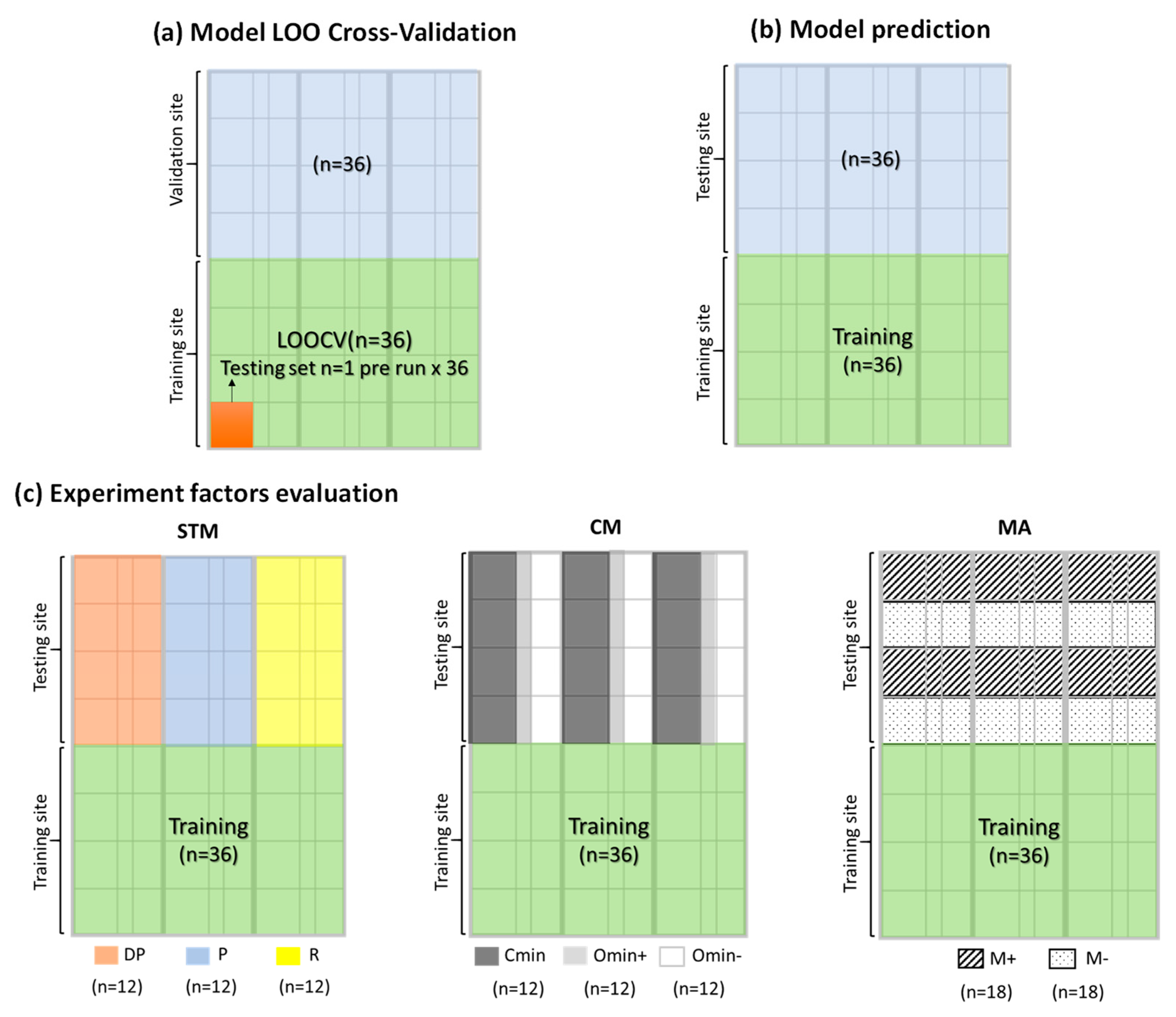
2.5.4. Model Evaluation

The evaluation was performed for LOO cross-validation, model prediction and experimental factor assessment (Figure 4). For the evaluation of each model, the accuracy evaluation method described by [66] was used. The models’ accuracies were measured by the coefficient of determination (R²) (Equation (1)) and normalized root means square error (NRMSE) (Equation (2)). The equations used are as follows:

$$R^2=1-\frac{\sum {\left({\widehat{y}}_i-y_i\right)}^2}{\sum {\left(y_i-\overline{y}\right)}^2}$$

(1)

$$NRMSE=\frac{\sqrt{\sum ({\left({\widehat{y}}_i-y_i\right)}^2)/n}}{\mathsf{\Delta }y}$$

(2)

where: $y_i$ represents the ith observation value of the training dataset; $\overline{y}$ represents mean value of the training dataset, ${\widehat{y}}_i$ is the model predictions, n is the number of observations, and $\mathsf{\Delta }y$ represents the difference between the maximum and minimum values of the training dataset.

3. Results

3.1. The Field Observation DM Data Analysis

The violin plot (Figure 5) displays the average true ground DM data collected from 144 plots taken during two harvest periods (1st cut and 2nd cut) of two experimental areas. Since the treatments were mixed with each plot, we only displayed the range of DM yield data, and grouped them by three farming operations, namely STM, CM, and MA. The potential interaction effects between treatments were not addressed during the analyses. The results of 1YC (Figure 5a) for STM showed that treatment P had a relatively lower DM than the R and DP treatments with a mean DM of 5195 kg ha-1. However, the effect of STM was noticeable in the two-year cultivation (2YC), in which the DM yield of R and P decreased in the 2YC field (Figure 5b). In terms of CM, DM from organically cultivated crops without mineral fertilizer (Omin-) can be expected to show lower yields in both fields. The DM yield of 2YC was slightly less than that of 1YC.

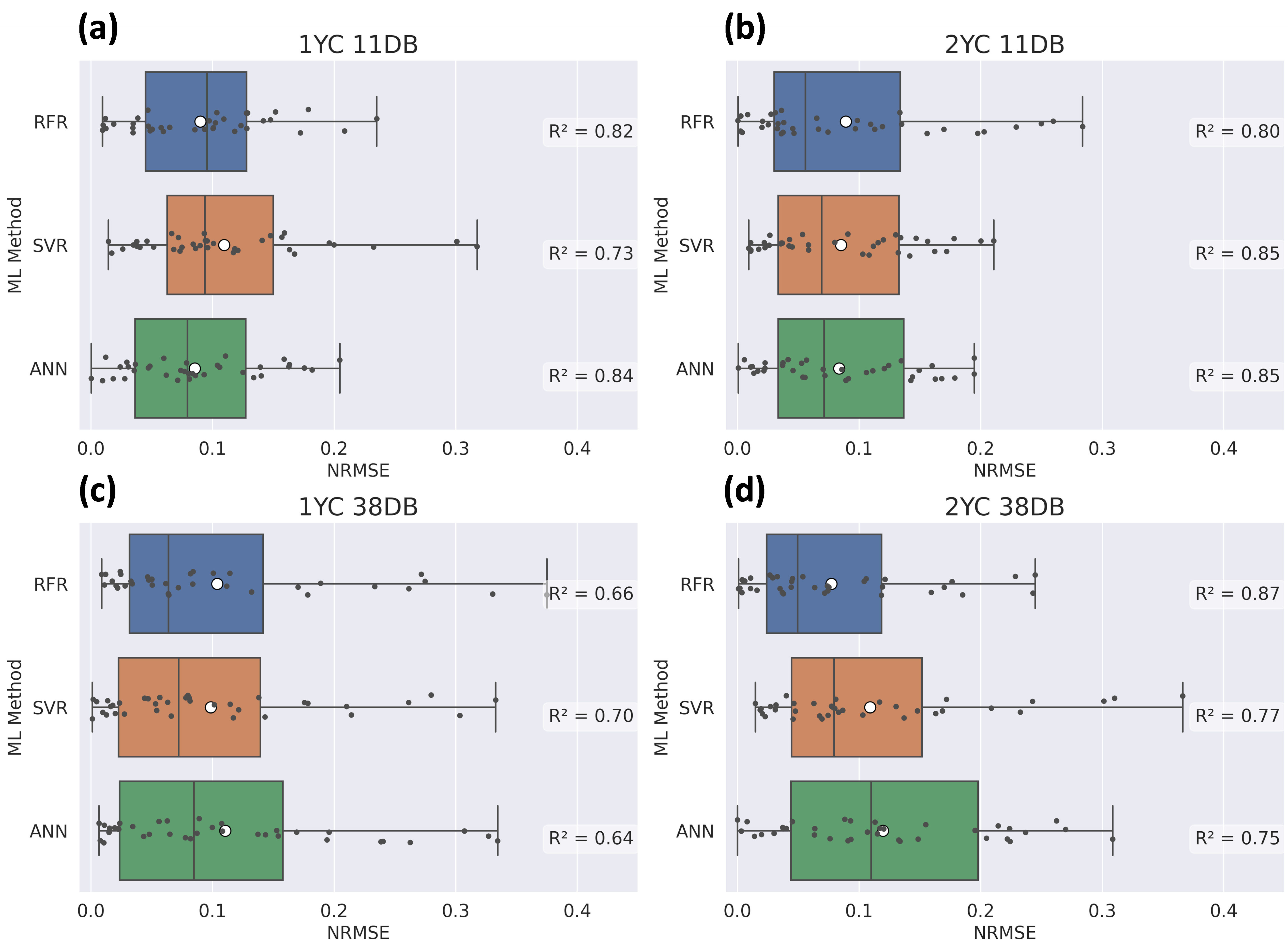
3.2. The Red Clover-Grass Mixture DM Modeling and LOOCV

For better evaluation evaluating of the model performance, LOOCV was firstly conducted in this research to assess three machine learning methods’ (RFR, SVR, and ANN) abilities to predict DM yield using six VIs. (Figure 4a) The distributions of R² and NRMSE values under thirty-six LOOCV iterations of the three models are shown in box plots (Figure 6). The results showed that in terms of flight dates, 11DB generally performed better than 38DB. In terms of model performance, ANN had the best performance in 11DB, with the highest R² values (1YC = 0.84, 2YC = 0.85), and the lowest median NRMSE with a stable distribution of outliers. RFR’s accuracy was slightly smaller than for ANN. In terms of regional prediction, 2YC was on average better than 1YC. Overall, the results of LOOCV showed that the three models have moderate to high accuracies in two locations and different flight dates, and the best R² values were observed in 2YC11D (0.80 to 0.85), while the worst were observed in 1YC38DB (0.64 to 0.70).

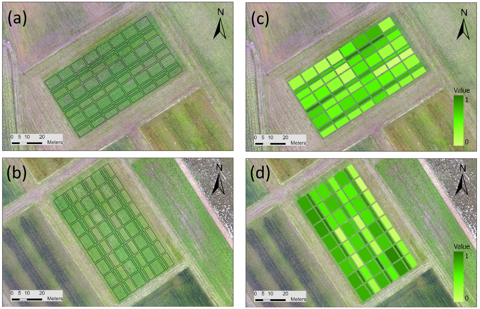
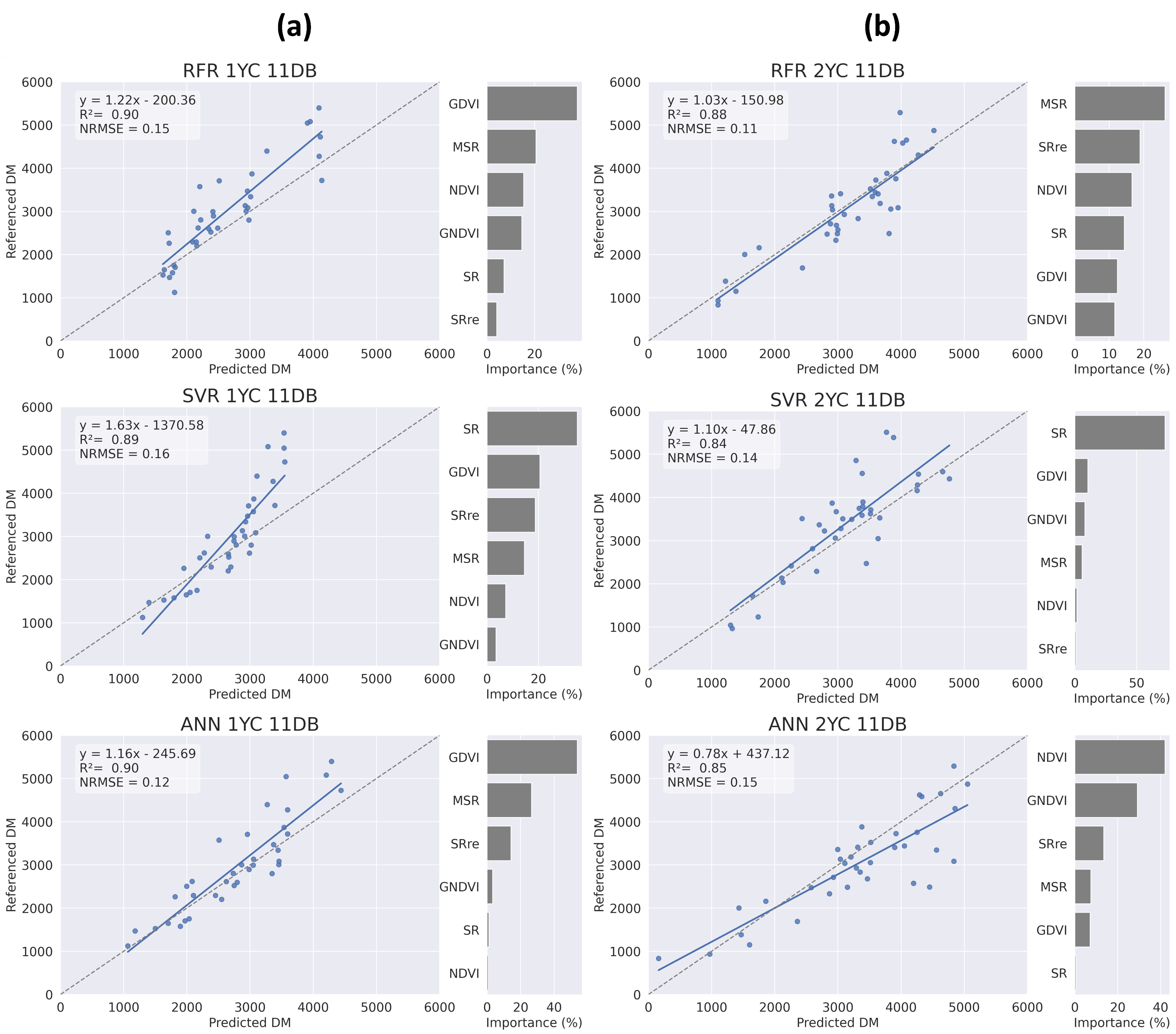
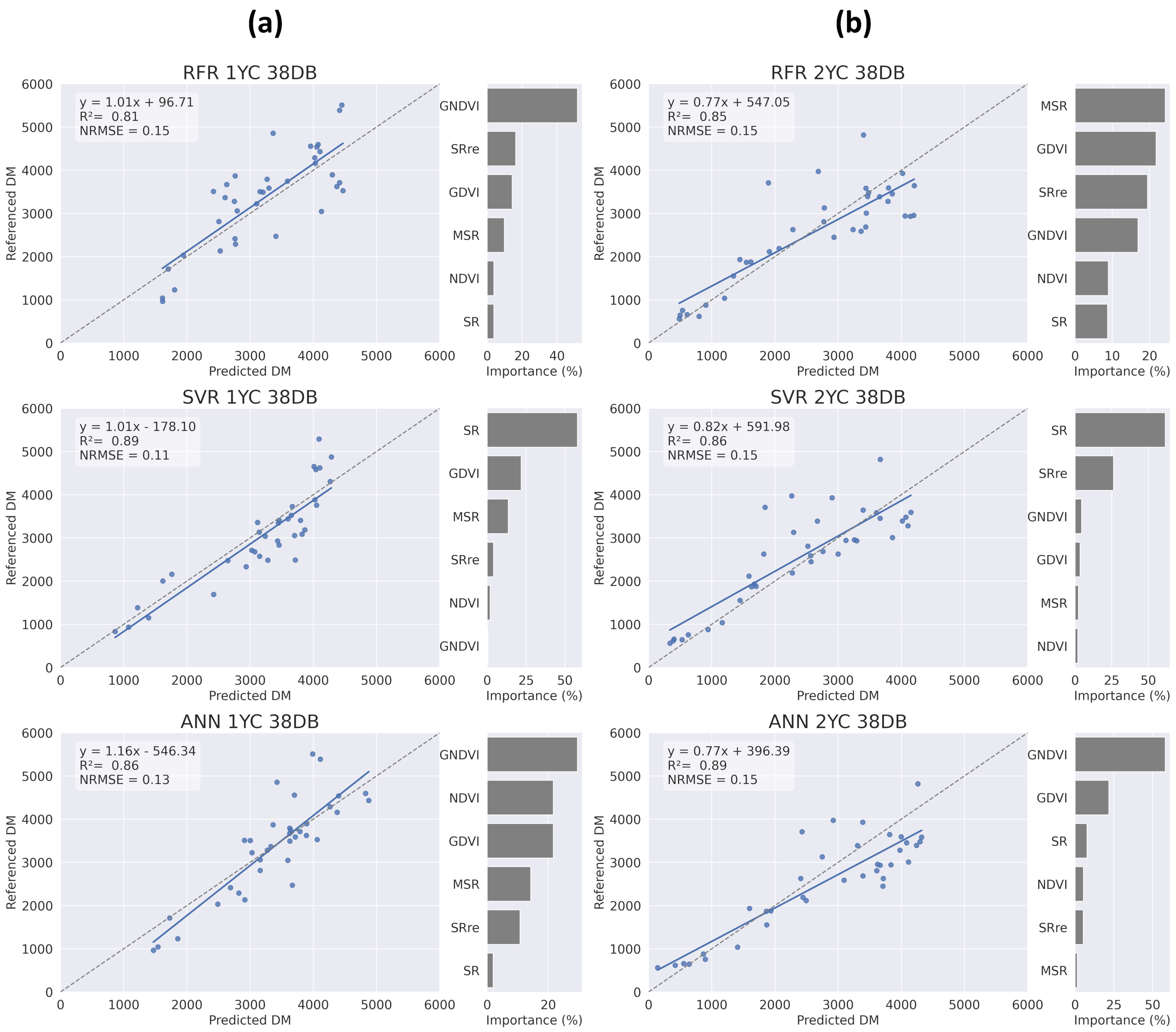
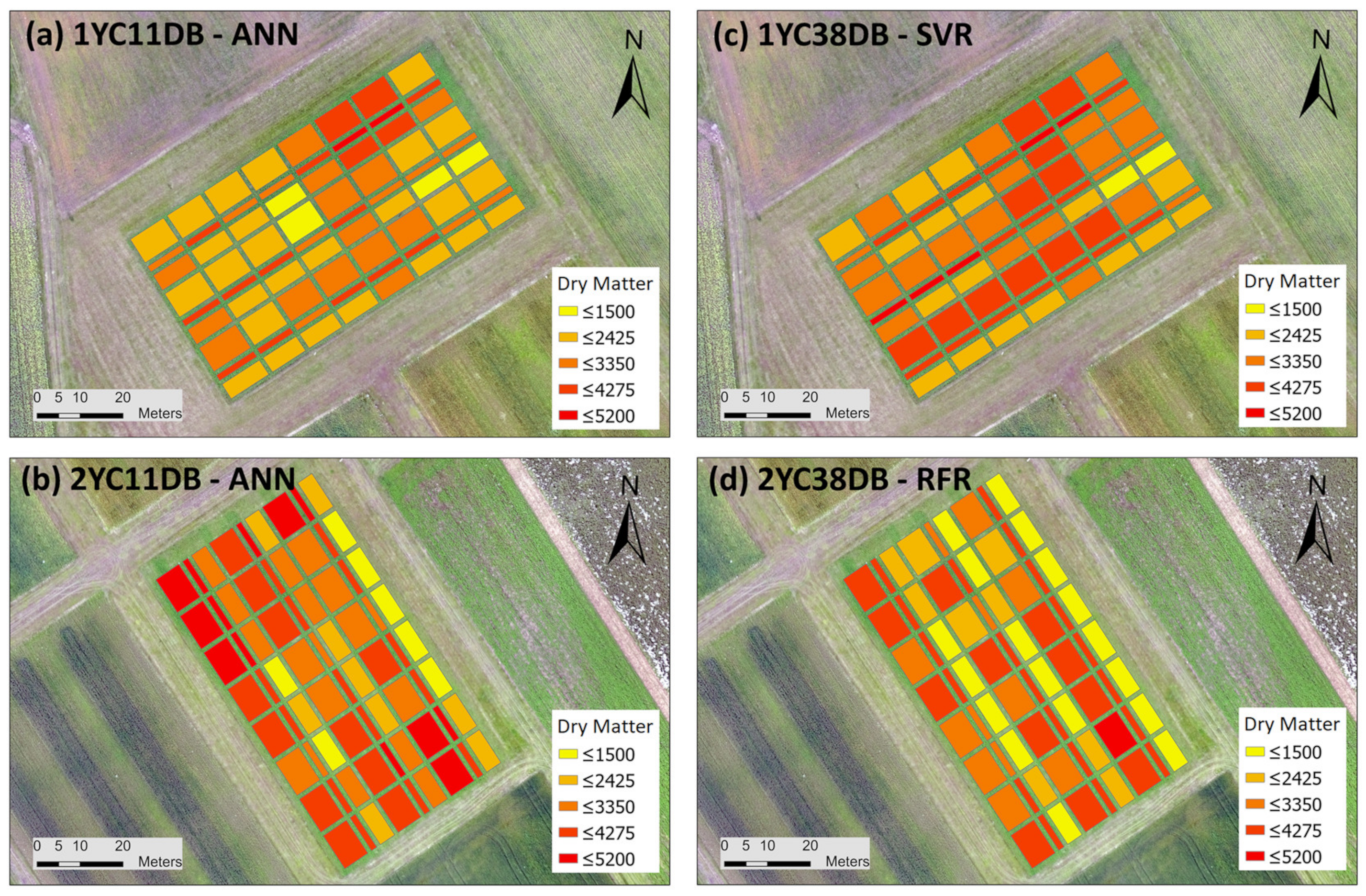
3.3. The Red Clover-Grass Mixture Model Prediction and Variable Importance

After the cross-validation, the training dataset (n = 36) was used for the calculation of models separately (Figure 4b). During the modeling phase, the appropriate combinations of the parameters of the data set were tested. The scatter plots with model predictions and observed DM values were compared to the 1:1 line, and their corresponding variable importance values are shown in Figure 7 and Figure 8.

Figure 7 shows three red clover-grass mixture DM models across the 1YC and 2YC fields where the images were captured eleven days before harvesting (11DB). The results indicate that, in 1YC11DB (Figure 7a), the ANN model had the lowest prediction errors (NRMSE = 0.12) and the highest R² value (0.90). RFR had a similar performance, but with higher NRMSE. Although the three models performed well, a slight uniform underestimation of DM yield appeared in both the RFR and ANN models. On the other hand, a non-uniform bias appeared in the SVR model, which overestimated small DM values and underestimated large DM values. According to the ranking of variable importance, GDVI and MSR provided higher contributions to the RFR and ANN models. Concerning the SVM model, larger contributions were found for SR and GDVI. The results of 1YC38DB (Figure 7b) show that the three models performed relatively well (R² from 0.84 to 0.88). The slope of RFR was closest to the 1:1 line, with the smallest NRMSE (0.11) and highest R² value (0.88); ANN and SVR had similar predictive capabilities. With regard to variable importance ranking, SVR showed similar results compared to 11DB with the highest contribution of SR, while in the results of RFR and ANN, the contribution of VIs did not show obvious similarity with the highest ranking in MSR and NDVI, respectively.

Figure 8 shows the behavior of predictive models using the thirty-eight days before harvest (38DB) datasets. The 1YC38DB results (Figure 8a) showed that SVR had the highest R² (0.89) and the smallest NRMSE (0.11), where the slope was close to the 1:1 line. In contrast, ANN and RFR relatively had weaker performances. However, the overall performance of the models for the 2YC dataset was slightly inferior to the result of 1YC, showing a higher bias of the slopes. In terms of 2YC38DB results (Figure 8b), ANN had the best performance among the three algorithms (R² = 0.89, NRMSE = 0.15). In the ranking of predictor variables in 1YC and 2YC, the GNDVI, MSR, NDVI, and SRre played crucial roles in both RFR and ANN models. Besides, the GNDVI was the most important variable in both 1YC and the model of ANN in the 2YC field. In contrast, SR stably ranked as the most important in the models of SVR, regardless of flight dates or regions.

Based on the evaluation of models (Figure 7 and Figure 8) and their suitability for different periods (Figure 6), we generated prediction maps (Figure 9) of DM yield for both experimental sites.

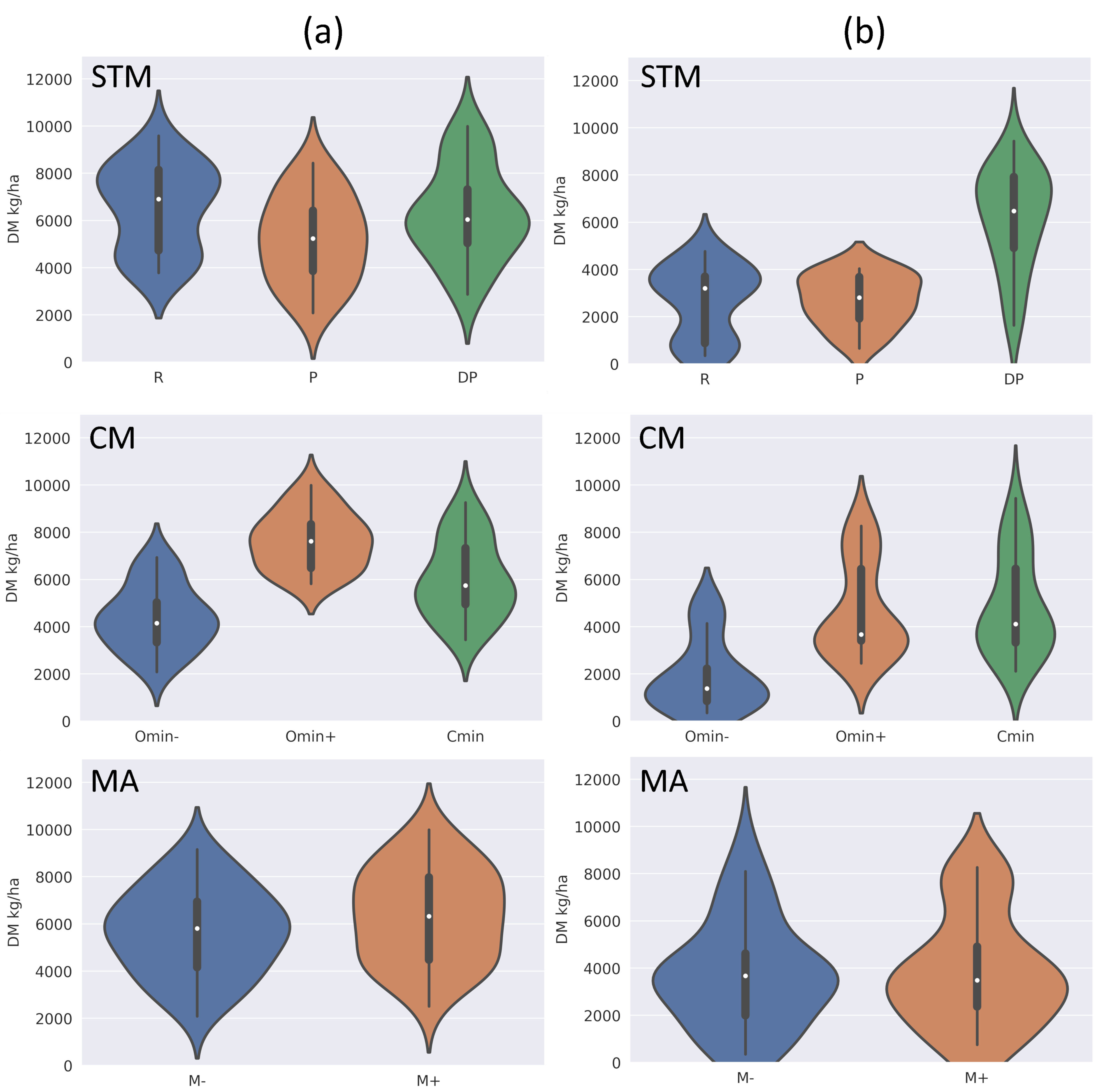
3.4. The Response of DM and VIs to Different Soil Tillage Methods (STM), Cultivation Method (CM), and Manure (MA) Treatments

To understand the detection capability of the relationship between VIs and DM yields under the influence of different soil tillage methods (STM), cultivation method (CM), and manure treatment (MA), three models were trained from previous 11DB datasets (Figure 4d). Testing sites were stratified sampling based on the three different farming operations to evaluate the predictive ability and sensitivity of detecting DM yields. The NRMSE and the R² values were performed for the goodness-of-fit measurement in 1YC (

Table 4. The evaluation of the models between observed and predicted DM yields under different experimental factors in 1YC11DB, the corresponding models for use was equivalent to Figure 7a. n = number of testing samples; R² = coefficient of determination; NRMSE = normalized root mean square error.

1YC11DB			RFR		SVR		ANN
Treatments		n	R2	NRMSE	R2	NRMSE	R2	NRMSE
STM	DP	12	0.85	0.26	0.81	0.34	0.92	0.29
	P	12	0.94	0.29	0.90	0.31	0.92	0.37
	R	12	0.90	0.20	0.85	0.23	0.90	0.19
CM	Cmin	12	0.75	0.31	0.62	0.48	0.80	0.31
	Omin+	12	0.69	0.31	0.74	0.26	0.60	0.47
	Omin−	12	0.89	0.18	0.85	0.27	0.82	0.20
MA	M+	18	0.88	0.19	0.82	0.21	0.86	0.23
	M−	18	0.91	0.21	0.84	0.22	0.88	0.24

) and 2YC(

Table 5. The evaluation of the models between observed and predicted DM yields under different experimental factors in 2YC11DB, the corresponding models for use was equivalent to Figure 8a. n = number of testing samples; R² = coefficient of determination; NRMSE = normalized root mean square error.

2YC11DB			RFR		SVR		ANN
Treatments		n	R2	NRMSE	R2	NRMSE	R2	NRMSE
STM	DP	12	0.93	0.14	0.92	0.13	0.96	0.08
	P	12	0.85	0.20	0.89	0.20	0.71	0.33
	R	12	0.91	0.16	0.94	0.16	0.87	0.24
CM	Cmin	12	0.92	0.19	0.96	0.19	0.76	0.25
	Omin+	12	0.70	0.24	0.81	0.25	0.49	0.35
	Omin−	12	0.90	0.14	0.93	0.12	0.91	0.15
MA	M+	18	0.79	0.17	0.81	0.16	0.69	0.24
	M−	18	0.95	0.10	0.95	0.11	0.96	0.11

) fields. Table 4 shows that, based on STM, the three models performed well in the DP, P, and R treatments, with the overall R² value ranging from 0.85 to 0.94, and NRMSE ranging from 0.19 to 0.37. In contrast, in CM, the performance of the three models showed lower accuracy in Cmin and Omin+. SVR had the worst performance with R² (0.62 and 0.74, respectively) and NRMSE (0.48 and 0.26). While in MA, the prediction ability of the three models was satisfactory. As Table 5 shows, the predictive ability of STM remained steady in the 2YC field. The R² ranges from 0.71 to 0.96, and NRMSE ranges from 0.08 to 0.33 in three models. In CM, Omin+ showed the worst R² and NRMSE values among other treatments with RFR (0.70 and 0.84, respectively) and, SVR (0.81 and 0.25) and ANN (0.49 and 0.35). In terms of the prediction ability of MA treatments, M- performed better than M+ with the R² values higher than 0.95, and the NRMSE values were less than or equal to 0.11 in all three models.

4. Discussion

This study has presented a rapid, non-destructive, low-cost framework for field-based red-clover DM yield modeling. The outputs have the potential to markedly assist agronomists and farmers in developing precise farming systems and increase the effective monitoring of environmental conditions.

4.1. Applicability of the Method

The prediction models covered three different agricultural operations (STM, CM, and MA) to represent the variable conditions in a practical farming system, which provided varied dry mass data to identify the robustness of the derived ML models. Acquisition of data conducted during two different periods offered a wider range of suitable monitoring capabilities. Three machine learning techniques (RFR, SVM, and ANN) were conducted to explore the DM yield prediction ability in legume pasture fields. All VI information was derived from four multispectral bands. Utilizing various Vis, which calculate the relative values or ratio among wavelengths can reduce the impact of radiance effects caused by individual reflectance spectra [67]. Besides, high-resolution multispectral imaging produces continuous and accurate indices in contrast to simple visual scores and rankings [68]. Consequently, no additional sensors were needed, which reduced measurement errors and increased cost-efficiency. It is important to consider that the eBee platform used in this study is potentially less practical for small farm area investigation (when compared to multi-rotor drones) [69]. The flexibility, however, in sensor systems, environmental capabilities, and increased flight durations could expand application to meet a diverse range of requirements [15] (e.g., larger-scale farmland or coverage area with shorter tasks duration); whilst still providing precise yield prediction accuracy required in our study.

4.2. The Impact of the Cultivated Period, Flight Times, and Farming Operations

The first specific objective was the development of red-clover biomass prediction models for one- and two-year cultivation periods, following common farming schedules in Northern Europe. Despite the results of the established models (Figure 7 and Figure 8), the prediction accuracy of 1YC (R² ranges from 0.81 to 0.90, NRMSE ranges from 0.11 to 0.15) and 2YC (R² ranges from 0.84 to 0.89, NRMSE ranges from 0.11 to 0.15) were both adequate. Nevertheless, the combination of clover-grass resulted in a heterogeneous canopy with the coverage of the two components. A previous mixed clover-grass study focused on canopy height (CH) modelling for DM yield prediction and showed the models performed better when established separately among the two species, and cannot be easily shifted to other grassland types owing to their structural characteristics [33]. Another study indicated that in terms of legume cover crops, the performance of NIR-based VIs did not perform much better than CH at the end of its crop cycle in terms of DM yield estimation [70]. This limitation of applying VIs in the mature growth stage of legumes does not necessarily impair the detection capacity, as forage biomass is usually harvested during the vegetative growth cycle [71]. A previous study found that although measurements performed at the ground-level were more accurate, the use of aerial systems was preferred since species identification was irrelevant when predicting the biomass of mixed-grass [72]. Therefore, these species-dependent VI phenomena seem to be a minor concern within the results presented in our study. We can infer that NIR-based VIs are suitable for the estimation of DM yields in one- and two-year cultivation periods in this study.

The second objective was to compare the impact of different pre-harvest flight dates on model estimation capabilities. The choice of flight timing was crucially matched with the spectral reflectance data during various growth periods. A previous study showed that the ideal period for forage crop assessment was one day before harvesting [32], whereas another study suggested that the targeted silage harvesting stage was favored [34]. Interestingly, studies focusing on other crop species have identified optimum monitoring periods in the case of maize yield prediction. The choice of performing a flight 100 days before harvest times had the best accuracy [73], whereas, for rice grain, it was optimal around the booting stage of growth [74]. In the case of our study on clover-grass mixes, the LOOCV and ML analysis demonstrate that the NRMSE average values from three models of 11DB were typically lower than those of 38DB (Figure 6). However, when compared to the bias of the slope of 11DB and 38DB from 1YC with the 1:1 line, 38DB provided a better model fit whilst at the same time being less prone to the under- or over-estimation of DM yield (Figure 7a and Figure 8a). Although the 11DB flight was in the red clover flowering stage, it seemed insignificantly influenced by the multispectral reflectance values since the flower size was small and normally less than 0.25 pixel in our study. Thus, the results indicate that in clover-grass mixture fields, the estimation ability is improved when UAS imagery is collected closer to the harvest period, but not later than the yellowing stage. Moreover, the results also indicate that the VIs derived from UAS images captured earlier than 38 days before harvest also have sufficient DM-yield estimation capacity and provide the potential to estimate DM earlier, while the accuracy might be partially lost.

The third objective was to explore, in detail, selected ML sensitivity regarding different farming operations. Relative research on the relationship between STM, CM, MA, and forage crop DM yields are still scarce in remote sensing studies. We redivided the testing site and stratified sampling the plots based on the differences in farming operations (Figure 4d), and the evaluation results of prediction ability based on STM was generally better in both 1YC and 2YC, followed by MA and CM treatments. Recently, remotely-sensed soil tillage quality evaluation on the bare soil level has contributed to compare several tillage techniques to increase the quality of farming work and energy conservation [75]. However, there are still few applications of the assessment of tillage methods and yield performance during the growth period of forage crops. The results of this study, which considered crop growth period when measuring DM yield, will assist farmers in making comparisons between several tillage methods for covering their basic agricultural needs.

On the other hand, a study confirmed that a biomass coverage index of 43.8% represents the best performance of disking operations [76]. Similarly in our study, a higher DM of 2YC red clover in DP treatment was observed (Figure 5b) and could be accurately predicted. However, the general predictive ability of CM was low, especially in the Omin+ treatment group, which may be attributed to the larger DM and spectral reflectance divergence of this area. In terms of tillage modeling results, previous studies have shown the non-tillage (NT) fields had more vigorous and abundant crops than conventional tillage (CT) methods, and the NIR-based VIs showed better discrimination performance than RGB-based VIs [26,77]. In our research, we have also found that the reduced tillage (R) areas yielded better accuracies, in comparative terms. A study of grassland DM yield estimation by a UAV-RGB camera showed different nitrogen fertilizer levels with its R² ranging from 0.57 to 0.70 [78]. Currently, adequate fertilizer estimation remains challenging in heterogeneous plant communities such as grasslands [32]. However, legume crops could provide more positive N balance input than mineral fertilization under various tillage conditions [79]. Although the input of N is not effectively quantified in this study, the DM yields of the various N input combinations could still be effectively predicted, which increases the viability of using non-destructive methods to quantify a range of, and distinct, N sources in future fertilizer management decisions.

4.3. The Machine Learning Methods

Machine learning techniques are still deemed to be novel in the realm of estimating grassland biomass [80]. The predictive ability of three broadly adopted and reliably implemented ML methods in clover-grass DM yield was promising in this study. ANN showed better predictive accuracy eleven days prior to harvest (11DB). This result is consistent with the LOO cross-validation results. The practicality and flexibility of ANN has previously been demonstrated in studies of grassland biomass estimation [81,82], and nitrogen and phosphorus concentration modeling in mixed-species environments [83,84]. Interestingly, within our study, RFR and SVR were shown to have increased predictive capability at 38DB; which is farther from the harvest period. Both RFR and SVR were also shown to have a promising potential in clover-grass biomass prediction applications, since they are fast and require fewer training samples, when compared to the ANN [80,85]. The overall accuracy of the three ML methods provided R² ranges from 0.81 to 0.90, and the NRMSE ranges from 0.11 to 0.15. These findings further support the asserted dominant ability of MLs as a perennial forage crop biomass estimator; demonstrated in this study for mixed-grass species.

4.4. Importance of Variable Rankings

Variable importance ranking is essential for predictor selection and model simplification normally. In our study, the results of ranking showed which VIs were able to capture most of the variability in vegetation characteristics from the grass fields. Different VI values at the level of leaf area indices were likely caused by the diverse canopy structures of clover (horizontal) and grass leaves (vertically orientated) [71]. A recent study confirmed that GNDVI is suitable as a biomass predictor for perennial forage crops, where R² = 0.80 for freshly-cut, and 0.66 for dry yields [86], as well as in the grain yield estimation in maize [87]. These results resemble the RFR and ANN modelling of this study, where the GNDVI, GDVI, and MSR had the highest average contributions. The weight of SR was generally low. A similar result was also found in a study of grass DM yield prediction by Partial Least Square (PLS) and RF techniques, where the above-mentioned VIs were relatively important variables, while SR yielded the worst prediction out of twelve VIs [22].

Other previous studies have indicated that NDVI is more commonly used for pasture biomass measurements [88,89], as well as in larger-scale grassland followed by seasonal monitoring [90]. However, the findings of this study indicate that NDVI may not be the most suitable VI, which was supported by a previous study [86]. This highlights the importance of considering the saturation, sensitivity, stages of crop development, canopy structure, and the type of environment when testing various vegetation indexes [15]. Our findings indicate that multispectral information based on NIR and the green band may be more suitable for DM yield prediction using RFR and ANN modelling. The exception, however, is the SR indices, which have the highest contribution consistently across all periods in the SVR modelling. This distinctive finding has yet to be found in similar crop studies in other literature. It is clear from our findings that more tests of VI should be conducted in studies to increase the collective understanding and improve the knowledge base.

4.5. The Limitations in This Study

In this study, the results may be limited by the red-clover and grass varieties present, and the study area investigated. This, however, can easily be addressed by including a wider range of species, and study regions, in future investigations. Further limitations may exist due to the inherent complexity and repeatability of field trial design, the small sample size, and the potential interaction effects between treatments; none of which are fully addressed through this study. Although RFR is known to be a suitable methodology for measuring smaller sample sizes [91], basic tree learners within the RFR algorithm benefited the performance of small datasets [62], whereas a higher number of sample points will typically lead to more accurate predictions. However, to address the potential for model over-fitting, we also implemented LOOCV in the training site. Here the results showed that the stability and divergence of variance were in an acceptable range. Nevertheless, increasing the number of samples will still be worth pursuing in future investigations, despite it creating an increased burden for onsite sampling and measurement.

5. Conclusions

Agriculture is experiencing a reimagined technological revolution supported by remote sensing technologies. In our study, UAS offers a significant sensor-based platform that supports VPT to develop current and future smart farming trends to achieve the assessment of eco-efficiency agriculture management practices and above-ground biomass estimation. It offers scientists and practitioners the capability to distinguish and compare trial changes, both spatially and temporally, for the monitoring and optimization of local agricultural practices. Our study has highlighted the potential for innovative machine learning methods to compensate for reduced sample sizes, reducing human efforts, and maximizing the utilization of available resources when implementing and simulating the actual activities in perennial clover-grass mixture trials.

We performed multispectral-UAS flights, under the one- and two-year cultivated red clover-grass mixture performance trials, within 38 to 11 days before the harvesting, with the GSD 10 cm and combined the resultant VI’s within multiple ML methods. Our findings present a robust DM yield prediction method, which can operate at the farm-scale; which is both non-destructive and cost-effective. The ML analysis results showed the best performance for ANN in the 11DB (R² = 0.90, NRMSE = 0.12), followed by RFR (R² = 0.90 NRMSE = 0.15), and SVM (R² = 0.86, NRMSE = 0.16). For VI performance, GNDVI and GDVI, and MSR performed well as predictors in ANN and RFR. While the prediction ability of models was being influenced by the farming operations, the stratified sampling based on STM provided a better model performance than CM and MA. The results indicate the potential of UAS to deal with complex experimental design development, such as tillage methods and varying fertilizer inputs.

However, the robustness and applicability of fertilizer quantification, and the mixed legume-grass species distribution detection, still remain to be addressed. Accurate and real-time phenotypic information of crops under diverse agri-environment schemes and their morphological and physiological states remains a further obstacle to be well-quantified by UAS, as well as providing theoretical and technical support for sustainable agricultural development in response to forage crop biomass/yield estimation in the future. The proposed methods in this study could also be improved further through the implementation of other practical techniques; such as texture analysis, which could offer the potential to measure spatial heterogeneity and improve accuracy [92]. In addition, further improvement could be developed by employing other ML network systems, like deep learning methods, to lower the misinterpretation rate [93]. However, this study does demonstrate the effectiveness, and potential of, short-term forage crop management monitoring by UAV to aid decision making, and presents a foundation on which to develop new possibilities for larger-scale UAV field-based phenotyping platforms to accelerate the crop breeding process.

References

1. Annicchiarico, P.; Barrett, B.; Brummer, E.C.; Julier, B.; Marshall, A.H. Achievements and Challenges in Improving Temperate Perennial Forage Legumes. Crit. Rev. Plant Sci. 2015, 34, 327–380. [Google Scholar] [CrossRef]
2. Bender, A.; Tamm, S. Seed yield of tetraploid red clover as influenced by cover crop management. Zemdirb. Agric. 2018, 105, 133–140. [Google Scholar] [CrossRef] [Green Version]
3. Thilakarathna, M.S.; McElroy, M.S.; Chapagain, T.; Papadopoulos, Y.A.; Raizada, M.N. Belowground nitrogen transfer from legumes to non-legumes under managed herbaceous cropping systems. A review. Agron. Sustain. Dev. 2016, 36, 58. [Google Scholar] [CrossRef] [Green Version]
4. Vleugels, T.; Amdahl, H.; Roldán-Ruiz, I.; Cnops, G. Factors Underlying Seed Yield in Red Clover: Review of Current Knowledge and Perspectives. Agronomy 2019, 9, 829. [Google Scholar] [CrossRef] [Green Version]
5. Arturi, M.J.; Aulicino, M.B.; Ansín, O.; Gallinger, G.; Signorio, R. Combining Ability in Mixtures of Prairie Grass and Clovers. Am. J. Plant Sci. 2012, 3, 1355–1360. [Google Scholar] [CrossRef] [Green Version]
6. Zarza, R.; Rebuffo, M.; La Manna, A.; Balzarini, M. Red clover (Trifolium pratense L.) seedling density in mixed pastures as predictor of annual yield. Field Crop. Res. 2020, 256, 107925. [Google Scholar] [CrossRef]
7. Doyle, C.; Topp, C. The economic opportunities for increasing the use of forage legumes in north European livestock systems under both conventional and organic management. Renew. Agric. Food Syst. 2004, 19, 15–22. [Google Scholar] [CrossRef]
8. Hanson, J.; Ellis, R.H. Progress and Challenges in Ex Situ Conservation of Forage Germplasm: Grasses, Herbaceous Legumes and Fodder Trees. Plants 2020, 9, 446. [Google Scholar] [CrossRef] [Green Version]
9. Carvell, C.; Roy, D.B.; Smart, S.M.; Pywell, R.F.; Preston, C.D.; Goulson, D. Declines in forage availability for bumblebees at a national scale. Biol. Conserv. 2006, 132, 481–489. [Google Scholar] [CrossRef]
10. Yang, X.; Drury, C.; Reynolds, W.; Reeb, M. Legume Cover Crops Provide Nitrogen to Corn During a Three-Year Transition to Organic Cropping. Agron. J. 2019, 111, 3253–3264. [Google Scholar] [CrossRef] [Green Version]
11. Yang, Y.; Reilly, E.C.; Jungers, J.M.; Chen, J.; Smith, T.M. Climate Benefits of Increasing Plant Diversity in Perennial Bioenergy Crops. One Earth 2019, 1, 434–445. [Google Scholar] [CrossRef]
12. Godfray, H.C.J.; Beddington, J.R.; Crute, I.R.; Haddad, L.; Lawrence, D.; Muir, J.F.; Pretty, J.; Robinson, S.; Thomas, S.M.; Toulmin, C. Food Security: The Challenge of Feeding 9 Billion People. Science 2010, 327, 812–818. [Google Scholar] [CrossRef] [PubMed] [Green Version]
13. Lüscher, A.; Mueller-Harvey, I.; Soussana, J.-F.; Rees, R.M.; Peyraud, J.-L. Potential of legume-based grassland–livestock systems in Europe: A review. Grass Forage Sci. 2014, 69, 206–228. [Google Scholar] [CrossRef] [PubMed]
14. Boelt, B.; Julier, B.; Karagić, Đ.; Hampton, J. Legume Seed Production Meeting Market Requirements and Economic Impacts. Crit. Rev. Plant Sci. 2014, 34, 412–427. [Google Scholar] [CrossRef]
15. Wachendorf, M.; Fricke, T.; Möckel, T. Remote sensing as a tool to assess botanical composition, structure, quantity and quality of temperate grasslands. Grass Forage Sci. 2018, 73, 1–14. [Google Scholar] [CrossRef]
16. Araus, J.L.; Cairns, J.E. Field high-throughput phenotyping: The new crop breeding frontier. Trends Plant Sci. 2014, 19, 52–61. [Google Scholar] [CrossRef]
17. Yang, G.; Liu, J.; Zhao, C.; Li, Z.; Huang, Y.; Yu, H.; Xu, B.; Yang, X.; Zhu, D.; Zhang, X.; et al. Unmanned Aerial Vehicle Remote Sensing for Field-Based Crop Phenotyping: Current Status and Perspectives. Front. Plant Sci. 2017, 8, 1111. [Google Scholar] [CrossRef]
18. Laidig, F.; Piepho, H.-P.; Drobek, T.; Meyer, U. Genetic and non-genetic long-term trends of 12 different crops in German official variety performance trials and on-farm yield trends. Theor. Appl. Genet. 2014, 127, 2599–2617. [Google Scholar] [CrossRef] [Green Version]
19. Lollato, R.P.; Roozeboom, K.; Lingenfelser, J.F.; Da Silva, C.L.; Sassenrath, G. Soft winter wheat outyields hard winter wheat in a subhumid environment: Weather drivers, yield plasticity, and rates of yield gain. Crop. Sci. 2020, 60, 1617–1633. [Google Scholar] [CrossRef]
20. Zhu-Barker, X.; Steenwerth, K.L. Nitrous Oxide Production from Soils in the Future. Chem. Bioavailab. Terr. Environ. 2018, 35, 131–183. [Google Scholar] [CrossRef]
21. Van Ittersum, M.K.; Cassman, K.G.; Grassini, P.; Wolf, J.; Tittonell, P.; Hochman, Z. Yield gap analysis with local to global relevance—A review. Field Crop. Res. 2013, 143, 4–17. [Google Scholar] [CrossRef] [Green Version]
22. Grüner, E.; Wachendorf, M.; Astor, T. The potential of UAV-borne spectral and textural information for predicting aboveground biomass and N fixation in legume-grass mixtures. PLoS ONE 2020, 15, e0234703. [Google Scholar] [CrossRef] [PubMed]
23. Costa, J.M.; Da Silva, J.M.; Pinheiro, C.; Barón, M.; Mylona, P.; Centritto, M.; Haworth, M.; Loreto, F.; Uzilday, B.; Turkan, I.; et al. Opportunities and Limitations of Crop Phenotyping in Southern European Countries. Front. Plant Sci. 2019, 10, 1125. [Google Scholar] [CrossRef] [PubMed] [Green Version]
24. Pieruschka, R.; Schurr, U. Plant Phenotyping: Past, Present, and Future. Plant Phenomics 2019, 2019, 1–6. [Google Scholar] [CrossRef]
25. Mozgeris, G.; Jonikavičius, D.; Jovarauskas, D.; Zinkevičius, R.; Petkevičius, S.; Steponavičius, D. Imaging from manned ultra-light and unmanned aerial vehicles for estimating properties of spring wheat. Precis. Agric. 2018, 19, 876–894. [Google Scholar] [CrossRef]
26. Yeom, J.; Jung, J.; Chang, A.; Ashapure, A.; Maeda, M.; Maeda, A.; Landivar, J. Comparison of Vegetation Indices Derived from UAV Data for Differentiation of Tillage Effects in Agriculture. Remote Sens. 2019, 11, 1548. [Google Scholar] [CrossRef] [Green Version]
27. Zhang, C.; Kovacs, J.M. The application of small unmanned aerial systems for precision agriculture: A review. Precis. Agric. 2012, 13, 693–712. [Google Scholar] [CrossRef]
28. Rouse, J.W.; Hass, R.H.; Schell, J.A.; Deering, D.W.; Harlan, J.C. Monitoring the Vernal Advancement and Retrogradation (Green Wave Effect) of Natural Vegetation; Final Report, RSC 1978-4; Texas A&M University: College Station, TX, USA, 1974. [Google Scholar]
29. Xue, J.; Su, B. Significant Remote Sensing Vegetation Indices: A Review of Developments and Applications. J. Sens. 2017, 2017, 1–17. [Google Scholar] [CrossRef] [Green Version]
30. Chao, Z.; Liu, N.; Zhang, P.; Ying, T.; Song, K. Estimation methods developing with remote sensing information for energy crop biomass: A comparative review. Biomass- Bioenergy 2019, 122, 414–425. [Google Scholar] [CrossRef]
31. Osco, L.P.; Ramos, A.P.M.; Pereira, D.R.; Moriya Érika, A.S.; Imai, N.N.; Matsubara, E.T.; Estrabis, N.; De Souza, M.; Junior, J.M.; Gonçalves, W.N.; et al. Predicting Canopy Nitrogen Content in Citrus-Trees Using Random Forest Algorithm Associated to Spectral Vegetation Indices from UAV-Imagery. Remote. Sens. 2019, 11, 2925. [Google Scholar] [CrossRef] [Green Version]
32. Lussem, U.; Bolten, A.; Gnyp, M.L.; Jasper, J.; Bareth, G. EVALUATION OF RGB-BASED VEGETATION INDICES FROM UAV IMAGERY TO ESTIMATE FORAGE YIELD IN GRASSLAND. ISPRS Int. Arch. Photogramm. Remote Sens. Spat. Inf. Sci. 2018, XLII-3, 1215–1219. [Google Scholar] [CrossRef] [Green Version]
33. Grüner, E.; Astor, T.; Wachendorf, M. Biomass Prediction of Heterogeneous Temperate Grasslands Using an SfM Approach Based on UAV Imaging. Agronomy 2019, 9, 54. [Google Scholar] [CrossRef] [Green Version]
34. Viljanen, N.; Honkavaara, E.; Näsi, R.; Hakala, T.; Niemeläinen, O.; Kaivosoja, J. A Novel Machine Learning Method for Estimating Biomass of Grass Swards Using a Photogrammetric Canopy Height Model, Images and Vegetation Indices Captured by a Drone. Agriculture 2018, 8, 70. [Google Scholar] [CrossRef] [Green Version]
35. Kaspersen, K.; Bakken, A.K. Evaluating an image analysis system for mapping white clover pastures. Acta Agric. Scand. Sect. B Plant Soil Sci. 2004, 54, 76–82. [Google Scholar] [CrossRef]
36. Abuleil, A.M.; Taylor, G.W.; Moussa, M. An Integrated System for Mapping Red Clover Ground Cover Using Unmanned Aerial Vehicles: A Case Study in Precision Agriculture. In Proceedings of the 2015 12th Conference on Computer and Robot Vision, Halifax, NS, Canada, 3–5 June 2015; pp. 277–284. [Google Scholar]
37. Oliveira, R.A.; Näsi, R.; Niemeläinen, O.; Nyholm, L.; Alhonoja, K.; Kaivosoja, J.; Jauhiainen, L.; Viljanen, N.; Nezami, S.; Markelin, L.; et al. Machine learning estimators for the quantity and quality of grass swards used for silage production using drone-based imaging spectrometry and photogrammetry. Remote Sens. Environ. 2020, 246, 111830. [Google Scholar] [CrossRef]
38. FAO. World Reference Base for Soil Resources. In World Soil Resources Report 103; FAO: Rome, Italy, 2006. [Google Scholar]
39. Poncet, A.M.; Knappenberger, T.; Brodbeck, C.; Fogle, J.M.; Shaw, J.N.; Ortiz, B.V. Multispectral UAS Data Accuracy for Different Radiometric Calibration Methods. Remote Sens. 2019, 11, 1917. [Google Scholar] [CrossRef] [Green Version]
40. senseFly. eBee: senseFly SA. Available online: https://www.sensefly.com/drones/ (accessed on 12 October 2019).
41. Metsar, J.; Kollo, K.; Ellmann, A. Modernization of the estonian national GNSS reference station network. Geod. Cartogr. 2018, 44, 55–62. [Google Scholar] [CrossRef] [Green Version]
42. Tomaštík, J.; Mokroš, M.; Surový, P.; Grznárová, A.; Merganič, J. UAV RTK/PPK Method—An Optimal Solution for Mapping Inaccessible Forested Areas? Remote Sens. 2019, 11, 721. [Google Scholar] [CrossRef] [Green Version]
43. Villoslada, M.; Bergamo, T.; Ward, R.; Burnside, N.; Joyce, C.; Bunce, R.; Sepp, K. Fine scale plant community assessment in coastal meadows using UAV based multispectral data. Ecol. Indic. 2020, 111, 105979. [Google Scholar] [CrossRef]
44. R Core Team. R: A Language and Environment for Statistical Computing; R Foundation for Statistical Computing: Vienna, Austria, 2020. [Google Scholar]
45. Hassan, M.A.; Yang, M.; Rasheed, A.; Yang, G.; Reynolds, M.; Xia, X.; Xiao, Y.; He, Z. A rapid monitoring of NDVI across the wheat growth cycle for grain yield prediction using a multi-spectral UAV platform. Plant Sci. 2019, 282, 95–103. [Google Scholar] [CrossRef]
46. Gitelson, A.A.; Kaufman, Y.J.; Stark, R.; Rundquist, D. Novel algorithms for remote estimation of vegetation fraction. Remote Sens. Environ. 2002, 80, 76–87. [Google Scholar] [CrossRef] [Green Version]
47. Tilly, N.; Hoffmeister, D.; Cao, Q.; Huang, S.; Lenz-Wiedemann, V.; Miao, Y.; Bareth, G. Multitemporal crop surface models: Accurate plant height measurement and biomass estimation with terrestrial laser scanning in paddy rice. J. Appl. Remote Sens. 2014, 8, 083671. [Google Scholar] [CrossRef]
48. Hunt, E.R.; Hively, W.D.; Daughtry, C.S.T.; Mccarty, G.W.; Fujikawa, S.J.; Ng, T.L.; Tranchitella, M.; Linden, D.S.; Yoel, D.W. Remote Sensing of Crop Leaf Area Index Using Unmanned Airborne Vehicles. In Proceedings of the Pecora 17 Symposium, Denver, CO, USA, 18 November 2008. [Google Scholar]
49. Serrano, L.; Filella, I.; Penuelas, J. Remote Sensing of Biomass and Yield of Winter Wheat under Different Nitrogen Supplies. Crop. Sci. 2000, 40, 723–731. [Google Scholar] [CrossRef] [Green Version]
50. Walsh, O.S.; Shafian, S.; Marshall, J.M.; Jackson, C.; McClintick-Chess, J.R.; Blanscet, S.M.; Swoboda, K.; Thompson, C.; Belmont, K.M.; Walsh, W.L. Assessment of UAV Based Vegetation Indices for Nitrogen Concentration Estimation in Spring Wheat. Adv. Remote Sens. 2018, 7, 71–90. [Google Scholar] [CrossRef] [Green Version]
51. Chen, J.M. Evaluation of Vegetation Indices and a Modified Simple Ratio for Boreal Applications. Can. J. Remote Sens. 1996, 22, 229–242. [Google Scholar] [CrossRef]
52. Gitelson, A.A.; Kaufman, Y.J.; Merzlyak, M.N. Use of a green channel in remote sensing of global vegetation from EOS-MODIS. Remote Sens. Environ. 1996, 58, 289–298. [Google Scholar] [CrossRef]
53. Sripada, R.P.; Heiniger, R.W.; White, J.G.; Meijer, A.D. Aerial Color Infrared Photography for Determining Early In-Season Nitrogen Requirements in Corn. Agron. J. 2006, 98, 968–977. [Google Scholar] [CrossRef]
54. Jordan, C.F. Derivation of Leaf-Area Index from Quality of Light on the Forest Floor. Ecology 1969, 50, 663–666. [Google Scholar] [CrossRef]
55. Gitelson, A.; Merzlyak, M.N. Spectral Reflectance Changes Associated with Autumn Senescence of Aesculus hippocastanum L. and Acer platanoides L. Leaves. Spectral Features and Relation to Chlorophyll Estimation. J. Plant Physiol. 1994, 143, 286–292. [Google Scholar] [CrossRef]
56. ESRI. ArcGIS PRO: Essential Workflows; ESRI: Redlands, CA, USA, 2016; Available online: https://community.esri.com/t5/esri-training-documents/arcgis-pro-essential-workflows-course-resources/ta-p/914710 (accessed on 1 June 2020).
57. Zheng, H.; Cheng, T.; Zhou, M.; Li, D.; Yao, X.; Tian, Y.; Cao, W.; Zhu, Y. Improved estimation of rice aboveground biomass combining textural and spectral analysis of UAV imagery. Precis. Agric. 2018, 20, 611–629. [Google Scholar] [CrossRef]
58. Poley, L.G.; McDermid, G.J. A Systematic Review of the Factors Influencing the Estimation of Vegetation Aboveground Biomass Using Unmanned Aerial Systems. Remote Sens. 2020, 12, 1052. [Google Scholar] [CrossRef] [Green Version]
59. Ma, L.; Li, M.; Ma, X.; Cheng, L.; Du, P.; Liu, Y. A review of supervised object-based land-cover image classification. ISPRS J. Photogramm. Remote Sens. 2017, 130, 277–293. [Google Scholar] [CrossRef]
60. Pilgrim, M. Dive into Python 3; Apress: New York, NY, USA, 2009. [Google Scholar]
61. Kearns, M.; Ron, D. Algorithmic Stability and Sanity-Check Bounds for Leave-One-Out Cross-Validation. Neural Comput. 1999, 11, 1427–1453. [Google Scholar] [CrossRef] [PubMed]
62. Breiman, L. Random Forests. Mach. Learn. 2001, 45, 5–32. [Google Scholar] [CrossRef] [Green Version]
63. Liu, T.; Abd-Elrahman, A.; Morton, J.; Wilhelm, V.L. Comparing fully convolutional networks, random forest, support vector machine, and patch-based deep convolutional neural networks for object-based wetland mapping using images from small unmanned aircraft system. GIScience Remote Sens. 2018, 55, 243–264. [Google Scholar] [CrossRef]
64. Shin, J.; Kim, H.J.; Park, S.; Kim, Y. Model predictive flight control using adaptive support vector regression. Neurocomputing 2010, 73, 1031–1037. [Google Scholar] [CrossRef]
65. He, Q. Neural Network and Its Application in IR; Graduate School of Library and Information Science, University of Illinois at Urbana-Champaign Spring: Champaign, IL, USA, 1999. [Google Scholar]
66. Yue, J.; Yang, G.; Li, C.; Li, Z.; Wang, Y.; Feng, H.; Xu, B. Estimation of Winter Wheat Above-Ground Biomass Using Unmanned Aerial Vehicle-Based Snapshot Hyperspectral Sensor and Crop Height Improved Models. Remote Sens. 2017, 9, 708. [Google Scholar] [CrossRef] [Green Version]
67. Li, B.; Xu, X.; Zhang, L.; Han, J.; Bian, C.; Li, G.; Liu, J.; Jin, L. Above-ground biomass estimation and yield prediction in potato by using UAV-based RGB and hyperspectral imaging. ISPRS J. Photogramm. Remote Sens. 2020, 162, 161–172. [Google Scholar] [CrossRef]
68. Wang, J.; Badenhorst, P.; Phelan, A.; Pembleton, L.; Shi, F.; Cogan, N.; Spangenberg, G.; Smith, K. Using Sensors and Unmanned Aircraft Systems for High-Throughput Phenotyping of Biomass in Perennial Ryegrass Breeding Trials. Front. Plant Sci. 2019, 10, 1381. [Google Scholar] [CrossRef] [PubMed]
69. Chaudhry, M.H.; Ahmad, A.; Gulzar, Q. A comparative study of modern UAV platform for topographic mapping. In Proceedings of the 10th IGRSM International Conference and Exhibition on Geospatial & Remote Sensing, Kuala Lumpur, Malaysia, 20–21 October 2020; Volume 540. [Google Scholar] [CrossRef]
70. Roth, L.; Streit, B. Predicting cover crop biomass by lightweight UAS-based RGB and NIR photography: An applied photogrammetric approach. Precis. Agric. 2017, 19, 93–114. [Google Scholar] [CrossRef] [Green Version]
71. Biewer, S.; Erasmi, S.; Fricke, T.; Wachendorf, M. Prediction of yield and the contribution of legumes in legume-grass mixtures using field spectrometry. Precis. Agric. 2009, 10, 128–144. [Google Scholar] [CrossRef]
72. Rueda-Ayala, V.P.; Peña, J.M.; Höglind, M.; Bengochea-Guevara, J.M.; Andújar, D. Comparing UAV-Based Technologies and RGB-D Reconstruction Methods for Plant Height and Biomass Monitoring on Grass Ley. Sensors 2019, 19, 535. [Google Scholar] [CrossRef] [Green Version]
73. Michez, A.; Bauwens, S.; Brostaux, Y.; Hiel, M.-P.; Garré, S.; Lejeune, P.; Dumont, B. How Far Can Consumer-Grade UAV RGB Imagery Describe Crop Production? A 3D and Multitemporal Modeling Approach Applied to Zea mays. Remote Sens. 2018, 10, 1798. [Google Scholar] [CrossRef] [Green Version]
74. Zhou, X.; Zheng, H.; Xu, X.; He, J.; Ge, X.; Yao, X.; Cheng, T.; Zhu, Y.; Cao, W.; Tian, Y. Predicting grain yield in rice using multi-temporal vegetation indices from UAV-based multispectral and digital imagery. ISPRS J. Photogramm. Remote Sens. 2017, 130, 246–255. [Google Scholar] [CrossRef]
75. Fanigliulo, R.; Antonucci, F.; Figorilli, S.; Pochi, D.; Pallottino, F.; Fornaciari, L.; Grilli, R.; Costa, C. Light Drone-Based Application to Assess Soil Tillage Quality Parameters. Sensors 2020, 20, 728. [Google Scholar] [CrossRef] [PubMed] [Green Version]
76. Fanigliulo, R.; Biocca, M.; Pochi, D. Effects of six primary tillage implements on energy inputs and residue cover in Central Italy. J. Agric. Eng. 2016, 47, 177–180. [Google Scholar] [CrossRef] [Green Version]
77. Ashapure, A.; Jung, J.; Yeom, J.; Chang, A.; Maeda, M.; Maeda, A.; Landivar, J. A novel framework to detect conventional tillage and no-tillage cropping system effect on cotton growth and development using multi-temporal UAS data. ISPRS J. Photogramm. Remote Sens. 2019, 152, 49–64. [Google Scholar] [CrossRef]
78. Lussem, U.; Bolten, A.; Menne, J.; Gnyp, M.L.; Bareth, G. Ultra-high spatial resolution uav-based imagery to predict biomass in temperate grasslands. ISPRS Int. Arch. Photogramm. Remote Sens. Spat. Inf. Sci. 2019, XLII-2/W13, 443–447. [Google Scholar] [CrossRef] [Green Version]
79. Wittwer, R.A.; van der Heijden, M.G. Cover crops as a tool to reduce reliance on intensive tillage and nitrogen fertilization in conventional arable cropping systems. Field Crop. Res. 2020, 249, 107736. [Google Scholar] [CrossRef]
80. Ali, I.; Greifeneder, F.; Stamenkovic, J.; Neumann, M.; Notarnicola, C. Review of Machine Learning Approaches for Biomass and Soil Moisture Retrievals from Remote Sensing Data. Remote Sens. 2015, 7, 16398–16421. [Google Scholar] [CrossRef] [Green Version]
81. Xie, Y.; Sha, Z.; Yu, M.; Bai, Y.; Zhang, L. A comparison of two models with Landsat data for estimating above ground grassland biomass in Inner Mongolia, China. Ecol. Model. 2009, 220, 1810–1818. [Google Scholar] [CrossRef]
82. Ali, I.; Cawkwell, F.; Dwyer, E.; Green, S. Modeling Managed Grassland Biomass Estimation by Using Multitemporal Remote Sensing Data—A Machine Learning Approach. IEEE J. Sel. Top. Appl. Earth Obs. Remote Sens. 2016, 10, 3254–3264. [Google Scholar] [CrossRef]
83. Mutanga, O.; Skidmore, A. Integrating imaging spectroscopy and neural networks to map grass quality in the Kruger National Park, South Africa. Remote Sens. Environ. 2004, 90, 104–115. [Google Scholar] [CrossRef]
84. Mutanga, O.; Kumar, L. Estimating and mapping grass phosphorus concentration in an African savanna using hyperspectral image data. Int. J. Remote Sens. 2007, 28, 4897–4911. [Google Scholar] [CrossRef]
85. Zhang, Z.; Masjedi, A.; Zhao, J.; Crawford, M.M. Prediction of sorghum biomass based on image based features derived from time series of UAV images. In Proceedings of the 2017 IEEE International Geoscience and Remote Sensing Symposium (IGARSS), Fort Worth, TX, USA, 23–28 July 2017; pp. 6154–6157. [Google Scholar] [CrossRef]
86. Théau, J.; Lauzier-Hudon, Étienne; Aubé, L.; Devillers, N. Estimation of forage biomass and vegetation cover in grasslands using UAV imagery. PLoS ONE 2021, 16, e0245784. [Google Scholar] [CrossRef]
87. Ramos, A.P.M.; Osco, L.P.; Furuya, D.E.G.; Gonçalves, W.N.; Santana, D.C.; Teodoro, L.P.R.; Junior, C.A.D.S.; Capristo-Silva, G.F.; Li, J.; Baio, F.H.R.; et al. A random forest ranking approach to predict yield in maize with uav-based vegetation spectral indices. Comput. Electron. Agric. 2020, 178, 105791. [Google Scholar] [CrossRef]
88. Insua, J.R.; Utsumi, S.A.; Basso, B. Estimation of spatial and temporal variability of pasture growth and digestibility in grazing rotations coupling unmanned aerial vehicle (UAV) with crop simulation models. PLoS ONE 2019, 14, e0212773. [Google Scholar] [CrossRef] [Green Version]
89. Lee, H.; Lee, H.-J.; Jung, J.-S.; Ko, H.-J. Mapping Herbage Biomass on a Hill Pasture using a Digital Camera with an Unmanned Aerial Vehicle System. J. Korean Soc. Grassl. Forage Sci. 2015, 35, 225–231. [Google Scholar] [CrossRef]
90. Ma, Q.; Chai, L.; Hou, F.; Chang, S.; Ma, Y.; Tsunekawa, A.; Cheng, Y. Quantifying Grazing Intensity Using Remote Sensing in Alpine Meadows on Qinghai-Tibetan Plateau. Sustainability 2019, 11, 417. [Google Scholar] [CrossRef] [Green Version]
91. Luan, J.; Zhang, C.; Xu, B.; Xue, Y.; Ren, Y. The predictive performances of random forest models with limited sample size and different species traits. Fish. Res. 2020, 227, 105534. [Google Scholar] [CrossRef]
92. Yang, M.-D.; Huang, K.-S.; Kuo, Y.-H.; Tsai, H.P.; Lin, L.-M. Spatial and Spectral Hybrid Image Classification for Rice Lodging Assessment through UAV Imagery. Remote Sens. 2017, 9, 583. [Google Scholar] [CrossRef] [Green Version]
93. Yang, M.-D.; Tseng, H.-H.; Hsu, Y.-C.; Tsai, H.P. Semantic Segmentation Using Deep Learning with Vegetation Indices for Rice Lodging Identification in Multi-date UAV Visible Images. Remote Sens. 2020, 12, 633. [Google Scholar] [CrossRef] [Green Version]
Figure 1. (a) The Agricultural Research Centre (ARC) is situated in Kuusiku, Estonia. A. The experiment layout containing three treatments: 1. soil tillage method (STM), 2. cultivation method (CM), and manure application (MA) for one-year cultivation (1YC) in Field A with a total of 72 observation plots, and two-year cultivation (2YC) in Field B equally with a total of 72 plots. For caption descriptions, see Table 1. (b) A visual demonstration of the different CM treatments within the 2YC DP area. (c) The eBee Plus device was used to capture the multispectral imaging data and the Airinov target was used for radiometric calibration in this study.
Remotesensing 13 01994 g001
Figure 2. The methodology flowchart of red clover-grass mixture DM modeling. The image processing rectangular dotted box contains all predictors extracted from the UAV images, and the modeling building, and evaluation rectangular dotted box contains all modeling methods and analysis procedure.
Remotesensing 13 01994 g002
Figure 3. A demonstration of VIs (GDVI as an example) zonal statistics in 1YC and 2YC fields. (a) RGB image with 1-meter buffer zone plot polygons from 1YC11DB, (b) RGB image with 1-meter buffer zone plot polygons from 2YC11DB, (c) GDVI zonal statistic with a region of interest (ROI) in 1YC11DB, and (d) GDVI zonal statistics with ROI from 2YC11DB.
Remotesensing 13 01994 g003
Figure 4. Examples of different sampling methods and regions in field 2YC, the training site (1/2, n = 36) contains two repeated trial plots. (a) The evaluation of RFR, SVR, and ANN using the cross-validation method LOOCV in the training site (1/2, n = 36) and validation site (1/2, n = 36). (b) Model construction including training site (1/2, n = 36) and testing site (1/2, n = 36). (c) Evaluation of the model efficiency across three different treatments: STM (n = 12 for each subset), CM (n = 12 for each subset), and MA (n = 18 for each subset).
Remotesensing 13 01994 g004
Figure 5. Violin plots of mean harvest results of clover-grass mixture dry matter (DM) yield in the (a) 1YC field and the (b) 2YC field, grouped by STM, CM, and MA farming operations. Biomass data were obtained during two separate harvests (1st cut and 2nd cut). The white dot indicates the median, while the thick black bars in the center show the interquartile range, the black line represents the rest of the distribution, and violins show point density and data distribution.
Remotesensing 13 01994 g005
Figure 6. Comparison of the NRMSE and R2 values resulting from 3 different ML methods (RFR, SVR, and ANN) of LOOCV in (a) 1YC11DB (b) 1YC38Db (c) 2YC11DB (d) 2YC38DB. Each model performed 36 times LOOCV calculations. The R2 for LOOCV was calculated using the average variance between the actual and prediction value for every iteration of the cross-validation. The black dots showed the NRMSE results of each cross-validation, and the white dots represent its average value. The median line in the box shows the middle value, and the interquartile range of the box (shown in blue, red, and green) represent the 25th to the 75th percentile.
Remotesensing 13 01994 g006
Figure 7. Regression plots of 1YC and 2YC fields based on RFR, SVR, and ANN methods in 11DB flight. The plots correspond to (a) 1YC11DB and (b) 2YC11DB. The horizontal bar plots on the right side of each graph shows the variable importance estimation based on the models. The horizontal axis in the scatter plots describes the predicted DM yield acquired from the model, and the vertical axis stands for the field-observed DM yield. The R2 = coefficient of determination, NRMSE = normalized root means squared error, and the black dotted line exemplifies the 1:1 slope.
Remotesensing 13 01994 g007
Figure 8. Regression plots of 1YC and 2YC fields based on RFR, SVR, and ANN methods in 38DB flight. The plots correspond to (a) 1YC38DB and (b) 2YC38DB. The horizontal bar plots on the right side of each graph shows the variable importance estimation based on the models. The horizontal axis in the scatter plots describes the predicted DM yield acquired from the model, and the vertical axis stands for the field observed DM yield. The R2 = coefficient of determination, NRMSE = normalized root means squared error, and the black dotted line exemplifies the 1:1 slope.
Remotesensing 13 01994 g008
Figure 9. The spatial testing (prediction) site mapping output of DM yields (kg ha−1) in 1YC and 2YC fields based on 11DB and 38DB flights by machine learning techniques at the plot level: (a) 1YC11DB, (b) 2YC11DB, (c) 1YC38DB, and (d) 2YC38DB. The best performing algorithm was chosen for each of the four categories, as shown in the previous results.
Remotesensing 13 01994 g009