Article

Constructing Adaptive Deformation Models for Estimating DEM Error in SBAS-InSAR Based on Hypothesis Testing

1
School of Geosciences and Info-Physics, Central South University, Changsha 410083, China
2
Spacety Co., Ltd., Changsha 410205, China
*
Author to whom correspondence should be addressed.
Remote Sens. 2021, 13(10), 2006; https://0-doi-org.brum.beds.ac.uk/10.3390/rs13102006
Submission received: 29 March 2021 / Revised: 14 May 2021 / Accepted: 17 May 2021 / Published: 20 May 2021

Abstract

:
The Interferometric Synthetic Aperture Radar (InSAR) technique has been widely used to obtain the ground surface deformation of geohazards (e.g., mining subsidence and landslides). As one of the inherent errors in the interferometric phase, the digital elevation model (DEM) error is usually estimated with the help of an a priori deformation model. However, it is difficult to determine an a priori deformation model that can fit the deformation time series well, leading to possible bias in the estimation of DEM error and the deformation time series. In this paper, we propose a method that can construct an adaptive deformation model, based on a set of predefined functions and the hypothesis testing theory in the framework of the small baseline subset InSAR (SBAS-InSAR) method. Since it is difficult to fit the deformation time series over a long time span by using only one function, the phase time series is first divided into several groups with overlapping regions. In each group, the hypothesis testing theory is employed to adaptively select the optimal deformation model from the predefined functions. The parameters of adaptive deformation models and the DEM error can be modeled with the phase time series and solved by a least square method. Simulations and real data experiments in the Pingchuan mining area, Gaunsu Province, China, demonstrate that, compared to the state-of-the-art deformation modeling strategy (e.g., the linear deformation model and the function group deformation model), the proposed method can significantly improve the accuracy of DEM error estimation and can benefit the estimation of deformation time series.

Graphical Abstract

1. Introduction

In recent decades, the interferometric synthetic aperture radar (SAR, InSAR) technique has been greatly developed and widely used to serve geohazard monitoring processes, such as those for mining subsidence [1,2,3], landslides [4,5,6], earthquakes [7,8,9], and volcano eruptions [10,11,12]. Especially when integrating multi-temporal SAR images with advanced time series InSAR (TS-InSAR) methods (e.g., persistent scatter (PS), small baseline subset (SBAS), and mixed PS/SBAS methods) [13,14,15,16,17], the inherent errors in a single interferogram (e.g., decorrelation noise and atmospheric delay) can be effectively mitigated, and simultaneously, the deformation time series of the study area can be obtained, which is of great significance for understanding the evolution process and mechanism of geohazards.
It is acknowledged that the interferometric phase includes not only the interested deformation component, but also undesirable noise components (e.g., decorrelation noise, atmospheric delay, and digital elevation model (DEM) error) [18]. Although the specific implementation process of different TS-InSAR methods is different, they should all first correct or weaken these noises before obtaining reliable deformation results. For example, decorrelation noise can be suppressed by multi-looking operation or the spatial filter [15]; stratified atmospheric delay can be mitigated by an elevation-dependent model [19,20] and turbulence atmospheric delay is generally reduced by a spatial-temporal filter or external meteorological datasets [14,21,22]; long-wavelength orbit error can be effectively alleviated by fitting second-order polynomials [23,24]. As for DEM error, it is an undesired component for deformation estimation. However, if the DEM error can be precisely estimated, it can be added back to the existing DEM data to generate a more accurate version of DEM data [25,26]. The DEM error-related interferometric phase is proportional to the spatial baseline of the interferogram [27,28,29,30]. In this case, the DEM error can be theoretically estimated by mathematical modeling. Generally, the deformation time series can be assumed to satisfy an a priori time-dependent deformation model, and the DEM error and model parameters can be simultaneously solved. In state-of-the-art deformation modeling strategies, a linear deformation model [13,31,32] is one of the most used a priori deformation models, which has been employed to obtain the deformation parameters associated with tectonic movement, ground subsidence, and so on. For specific deforming situations (e.g., permafrost and active caldera), we can employ the period model [33], cubic model [15], or even the function group deformation model [34]. Note that the accuracies of the DEM error and the final deformation time-series are both dependent on the reliability of the a priori deformation model. However, in reality it is impracticable to understand the real deformation evolution beforehand, and it is difficult to find a reliable model that can fit the long time-span deformations. Although the DEM error can also be estimated by a nonparametric estimator (e.g., independent component analysis [35]), the performance of this estimator may be degraded in some situations when only a small number of observations in space are available or high-level noise and outliers exist in observations [36].
To tackle the aforementioned problem, relative to the deformation model, we propose a method to construct adaptive deformation models for estimating DEM error based on hypothesis testing in the framework of the SBAS-InSAR method. The basis of this method is that the natural ground deformation is usually a time-dependent smooth process [37], and the increasing temporal sampling of SAR images (e.g., Sentinel-1 SAR images) will make the deformations at adjacent acquisitions more consistent with this smooth process. Under these circumstances, if the whole time span is divided into several small time spans, a set of time-dependent functions (e.g., cubic polynomials and periodic function) can be used to fit the deformation time series in each small time span. However, too many time-dependent functions easily induce the overfitting of deformation time series, resulting in possible biases in the estimation of parameters. Hypothesis testing is an inferential statistical process that uses sample data to assess the plausibility of established null hypotheses, which has been used to adaptively determine the influencing factors of the deformation model [38,39,40]. Therefore, we employed hypothesis testing here to statistically test the parameter significance of the predefined functions, and then those significant parameters were adaptively selected to construct the final deformation model used to assist the estimation of DEM error. This self-adaptive deformation model not only avoids the error induced by the simple model that cannot effectively fit the true deformation, but also reduces the possible overfitting error of the too complex function group.
To validate the superiority of the proposed method, both simulations and real data experiments over the Pingchuan mining area were conducted. The Pingchuan mining area belongs to the Jingyuan coal field, which is one of the most important coal bases in the Gansu Province, China. Coal mining began in this area in as early as the 1970s, and the ground deformations time series are significant and nonlinear, as a result of the continuous mining activities.
The rest of this paper is structured as follows: Section 2 presents the proposed method of constructing adaptive deformation models based on hypothesis testing; then, the validation of the proposed method with simulated experiments and real data experiments in the Pingchuan mining area, Gaunsu, China, is shown in Section 3. Finally, some discussions are given and conclusions drawn in Section 4 and Section 5, respectively.

2. Methodology

Since the proposed method is based on the framework of the SBAS-InSAR method, we first introduce the basic idea of the SBAS-InSAR method in Section 2.1; then, details about the proposed method for constructing adaptive deformation models, based on hypothesis testing, are subsequentially presented in Section 2.2, Section 2.3 and Section 2.4.

2.1. Basic Idea of the SBAS-InSAR Method

In the SBAS-InSAR method, multi-prime interferograms with short spatial–temporal baselines are used for the estimation of deformations, which can significantly suppress the decorrelation noise in the vegetation area, compared to single-prime interferograms. Generally, the interferometric phase between two SAR images for a pixel can be expressed as [18]:
δ φ = δ φ d e f + δ φ t o p o + δ φ o r b + δ φ a t m + δ φ n o i s e
where δ φ represents the observed interferometric phase, δ φ d e f represents the surface deformation phase along the line-of-sight (LOS) direction during two acquisitions, δ φ t o p o represents the topographic residuals phase due to the DEM error, δ φ o r b represents the orbit error-related phase and can be modeled by second-order polynomials, δ φ a t m represents the difference in atmospheric delay between two acquisitions, and δ φ n o i s e represents the random noise.
Assuming that the orbit error phase is mostly removed by existing methods and the atmospheric delay can be regarded as random noise in the temporal domain, the interferometric phase can be written as:
δ φ = δ φ d e f + δ φ t o p o + δ φ n o i s e
where the topographic residuals phase can be modeled as [27]:
δ φ t o p o = 4 π λ B r s i n θ d z
where B is the perpendicular spatial baseline between the two acquisitions, r is the slant range between the SAR antenna and ground surface, θ is the looking angle, and d z represents the DEM error. Since the observation system that includes both the deformation time series and the DEM error is underdetermined, an a priori deformation model is commonly employed in the SBAS-InSAR method before the estimation of the final deformation time series. In the SBAS-InSAR method, a linear model is generally employed to fit the deformation time series [15,41]:
δ φ d e f = 4 π Δ t λ v
where λ is the radar wavelength, Δ t is the temporal baseline of the interferogram, and v is the unknown deformation model parameter.
Given that there are M interferograms obtained from N SAR images based on the spatial–temporal baseline thresholds, the DEM error and the deformation model parameters can be solved with Equation (2) in a least-squares sense. Then, the DEM error phase components are removed from the M interferograms, after which the interferogram residuals are used to estimate the N deformation time series by taking the first acquisition as the reference.
In this paper, the innovation lies in the adaptive construction of the deformation model (i.e., Equation (4)). To this aim, phase time series were firstly estimated from the multi-prime unwrapped interferograms, which is more appropriate for the conduction of hypothesis testing compared to interferograms (Section 2.2). Secondly, hypothesis testing was employed to adaptively choose the deformation models from a set of time-dependent functions (Section 2.3). Finally, the adaptive deformation model parameters and the DEM error were simultaneously estimated based on a least-squares method (Section 2.4).

2.2. Derivation of Phase Time Series from Multi-Prime Interferograms

Before constructing the adaptive deformation model based on hypothesis testing, multi-prime unwrapped interferograms are used to obtain the phase time series, which can decrease the sensitivity of parameter estimation to the interferogram network [30]. The relationship between the M unwrapped phases δ φ = [ δ φ 1 , δ φ 2 , , δ φ M ] T and the N phase time series φ = [ φ 1 , φ 2 , , φ N ] T can be modeled as
δ φ = B φ
where B denotes the design matrix between the interferograms and the phase time series. If the M interferograms belong to a single baseline subset, Equation (5) can be directly solved by the least-squares method (i.e., Equation (6)).
φ = ( B T B ) 1 B T δ φ
However, if not, the singular value decomposition (SVD) or the iteratively reweighted least-squares (IRLS) methods can used to estimate the unknowns.
Since the characteristics of real ground deformation are complex and changeable, it is difficult to fit the deformations by only one model for long time series. To choose a model that is closer to the real deformation, the observations are divided into different groups according to a fixed time span. Moreover, the adjacent groups have 20% overlapping observations to allow different groups to constrain one another. Supposing there are J groups, the number of observations in each group is n j , and the number of overlapping observations is l . Generally, the time series in one year are taken as a group, and details about the determination of the time span for one group are presented in Section 4.1.

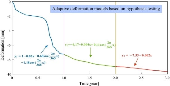
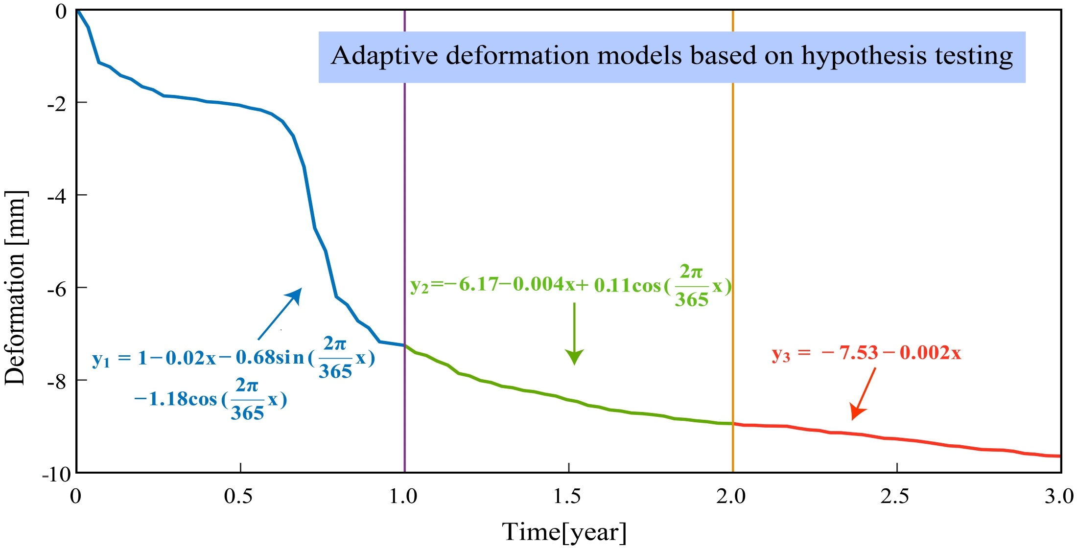
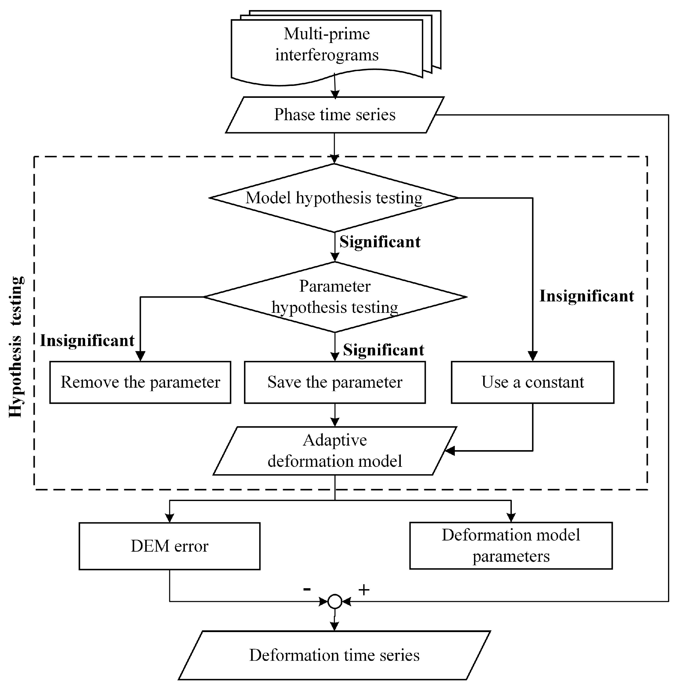
2.3. Construction of the Adaptive Deformation Model Based on Hypothesis Testing

In this paper, the functions in Equation (7) are used as the original deformation models:
φ j = k j + v j t j + a j t j 2 + Δ a j t j 3 + s j × s i n ( 2 π T × t j ) + c j × c o s ( 2 π T × t j )
where k j is the constant term, v j is the mean velocity, a j is the acceleration, Δ a j is the acceleration variation, s j and c j are the coefficients of the sine and cosine functions, T is defined as 365 days, φ j = [ φ 1 j , φ 2 j , , φ n j j ] T represents the phase values of the n j phase time series in the j th group, t j = [ t 1 j , t 2 j , , t n j j ] T represents the corresponding time of φ j , and j = 1 , 2 , , J . Let b 1 j = t j , b 2 j = t j 2 , b 3 j = t j 3 , b 4 j = s i n ( 2 π T × t j ) , b 5 j = c o s ( 2 π T × t j ) ; Equation (7) can be written as:
φ j = k j + v j × b 1 j + a j × b 2 j + Δ a j × b 3 j + s j × b 4 j + c j × b 5 j
where k j , v j , a j , Δ a j , s j , c j are the unknown deformation model parameters; b u j = [ b u 1 j , b u 2 j , , b u n j j ] T is the coefficient of the unknown parameter. To make it clear to the reader, the complete form of Equation (8) is:
[ φ 1 j φ 2 j φ n j j ] = [ 1 b 11 j b 21 j b 31 j b 41 j b 51 j 1 b 12 j b 22 j b 32 j b 42 j b 52 j           1 b 1 n j j b 2 n j j b 3 n j j b 4 n j j b 5 n j j ] [ k j v j a j Δ a j s j c j ]
Moreover, two variables are defined for better expression of the following process.
B 0 j = [ 1 b 11 j b 21 j b 31 j b 41 j b 51 j 1 b 12 j b 22 j b 32 j b 42 j b 52 j           1 b 1 n j j b 2 n j j b 3 n j j b 4 n j j b 5 n j j ] , X 0 j = [ x 0 j x 1 j x 2 j x 3 j x 4 j x 5 j ] = [ k j v j a j Δ a j s j c j ]
Then, hypothesis testing is conducted for each group to test the significance of the coefficient of time-dependent variables in Equation (8) [38,39]. For generality, the process of hypothesis testing for the j th group is illuminated as follows.
First, the significance of the original model (i.e., Equation (8)) should be tested. The null hypothesis is:
H 0 : [ x 1 j , x 2 j , , x p 0 j j ] T = [ 0 , 0 , 0 , 0 , 0 ] T
If H 0 can be accepted, the original deformation model is considered non-significant, and vice versa. To test the significance of the deformation model, the following statistical variable is established [38,39]:
F = S S R / p 0 j S S E / ( n j p 0 j 1 ) F ( p 0 j , n j p 0 j 1 )
where F ( n 1 , n 2 ) is the F distribution whose degree of freedom is n 1 and n 2 , S S R = i = 1 n j ( φ ^ i j φ ¯ j ) 2 ,   S S E = i = 1 n j ( φ i j φ ^ i j ) 2 , φ ¯ j is the mean value of φ j , and φ ^ i j is the re-estimated value of φ i j based on the unknown estimation. The deformation model is significant when F > F α ( p 0 j , n j p 0 j 1 ) , where α is the significance level, and can usually be set as 0.01.
However, it may happen that the model is insignificant due to the existence of severe noise (e.g., atmospheric delay). In this case, the following hypothesis testing process would not be conducted, and the null hypothesis H 0 would be adopted, which means that a constant model is used to fit the deformations.
Second, if the deformation model is significant, the significance of each deformation model parameter, except the constant term, will be tested. The null hypothesis is:
H 0 : x u j = 0 , u = 1 , 2 , , p 0 j
If H 0 is accepted, x u j is considered insignificant and the parameter x u j should be removed from the model, and vice versa. Similarly, the following statistical variable is established [38,39]:
T u = x ^ u j / q u u σ ^ t ( n j p 0 j 1 )
where x ^ u j is the estimation of x u j , q u u is the ( u + 1 ) th diagonal element of Q = ( ( B j ) T B j ) 1 ,   σ ^ = 1 n j p 0 j 1 i = 1 n j ( φ i j φ ^ i j ) 2 , and t ( n ) represents the t distribution whose degree of freedom is n . The corresponding parameter is significant when | T u | > t α 2 ( n j p j 1 ) , where α is the significance level, and can usually be set as 0.01.
After hypothesis testing of all model parameters, a new deformation model can be obtained by removing the insignificant parameters from Equation (8):
φ j = B j X j
where B j and X j can be obtained by removing the corresponding parts of the insignificant parameters from B 0 j and X 0 j , respectively.
The deformation model of each group of phase time series can be adaptively constructed based on the aforementioned process (i.e., Equations (8)–(14)), and are used in the following subsection to simultaneously estimate the deformation model parameters and the DEM error.

2.4. Estimation of the Deformation Model Parameters and DEM Error

The DEM error-related phase is usually small in phase time series compared to the deformation signal, and the natural ground deformation is usually a time-dependent smooth process. In this paper, the phase differences of the adjacent acquisitions are taken as the observations to increase the proportion of the DEM error-related phase among the observations. Since the phase time series are divided into several overlapping groups, there are two kinds of observation equations that can be established, including (1) the observation equations for each group related to the DEM error and their individual model parameters of each group, and (2) the observation equations in the overlapping time span between two adjacent groups. The deformation time series should be equal for the two sets of model parameters of the two adjacent groups, based on which the latter kind of observation equation can be established.
As for the first kind of observation equation, by referring to Equation (2), we can model the j th group of observations as:
Δ φ j = Δ φ d e f o j + Δ φ topo j
Based on the adaptive deformation model constructed in the last subsection and the relationship between the DEM error d z and the related phase Δ φ t o p o j , Equation (15) can be rewritten as:
Δ φ j ( n j 1 ) × 1 = [ Δ B j ( n j 1 ) × p j , c j ( n j 1 ) × 1 ] [ X j p j × 1 d z ]
where:
Δ φ j = [ φ 2 j φ 1 j φ 3 j φ 2 j φ n j j φ n j 1 j ] , Δ B j = [ b 12 j b 11 j b 22 j b 21 j b p j 2 j b p j 1 j b 13 j b 12 j b 23 j b 22 j b p j 3 j b p j 2 j       b 1 n j j b 1 ( n j 1 ) j b 2 n j j b 2 ( n j 1 ) j b p j n j j b p j ( n j 1 ) j ] c j = [ 4 π λ B ( t 2 j ) B ( t 1 j ) r sin θ 4 π λ B ( t 3 j ) B ( t 2 j ) r sin θ 4 π λ B ( t n j j ) B ( t n j 1 j ) r sin θ ] ,   X j = [ x 1 j x 2 j x p j j ]
and [ φ 1 j , φ 2 j , , φ n j j ] is the phase time series observations in the j th group, while [ b 1 i j , b 2 i j , , b p j i j ] is the time-dependent coefficient (see Equation (7)) representing the relationship between the deformation model parameters and the i th observation of the j th group, [ x 1 j , x 2 j , , x p j j ] T is the deformation model parameter, B ( t i j ) is the perpendicular baseline of the SAR image at the i th acquisition of the j th group t i j relative to the initial reference SAR image, with i = 1 , 2 , , n j , d z is the DEM error, λ is the wavelength of the SAR signal,   r is the slant distance between the sensor and the ground point, and θ is the incident angle. In summary, the number of this first observation equation is j = 1 J ( n j 1 ) .
In the overlapping region between two adjacent groups, the following pseudo-observation equations can be established based on the constraint that the deformation time series should be equal for the two sets of model parameters:
[ 0 ] ( l 1 ) × 1 = [ Δ B o v e r l a p j ,   Δ B o v e r l a p j + 1 ] ( l 1 ) × ( p j + p j + 1 ) [ X j X j + 1 ] ( p j + p j + 1 ) × 1
where:
Δ B o v e r l a p j = [ b 1 ( n j l + 1 ) j b 1 ( n j l ) j b 2 ( n j l + 1 ) j b 2 ( n j l ) j b p j ( n j l + 1 ) j b p j ( n j l ) j b 1 ( n j l + 2 ) j b 1 ( n j l + 1 ) j b 2 ( n j l + 2 ) j b 2 ( n j l + 1 ) j b p j ( n j l + 2 ) j b p j ( n j l + 1 ) j       b 1 n j j b 1 ( n j 1 ) j b 2 n j j b 2 ( n j 1 ) j b p j n j j b p j ( n j 1 ) j ] Δ B o v e r l a p j = [ b 12 j + 1 b 11 j + 1 b 22 j + 1 b 21 j + 1 b p j + 1 2 j + 1 b p j + 1 1 j + 1 b 13 j + 1 b 12 j + 1 b 23 j + 1 b 22 j + 1 b p j + 1 3 j + 1 b p j + 1 2 j + 1       b 1 l j + 1 b 1 ( l 1 ) j + 1 b 2 l j + 1 b 2 ( l 1 ) j + 1 b p j + 1 l j + 1 b p j + 1 ( l 1 ) j + 1 ]
and l is the number of overlapping observations between two adjacent groups. In summary, the number of this second observation equation is ( l 1 ) × ( J 1 ) .
Combining Equations (16) and (17) the following system can be obtained, from which the deformation model parameters and the DEM error can be simultaneously estimated based on the least-squares method.
[ Δ φ 1 Δ φ 2 Δ φ J 1 Δ φ J 0 0 ] = [ Δ B 1 0 0 0 c 1 0 Δ B 2 0 0 c 2           0 0 Δ B J 1 0 c J 1 0 Δ B o v e r l a p 1   0 0 Δ B o v e r l a p 2   0 0 0   Δ B o v e r l a p J 1 Δ B J 0   Δ B o v e r l a p J c J 0   0 ] [ X 1 X 2 X J 1 X J d z ]
After the correction of the DEM error from the phase time series, deformation time series can be obtained. In addition, if the deformation residuals are still severely affected by atmospheric delays, a step to mitigate the atmospheric delays is necessary [14,22]. The overall processing chain of the proposed method for constructing an adaptive deformation model based on hypothesis testing is shown in Figure 1.

3. Results

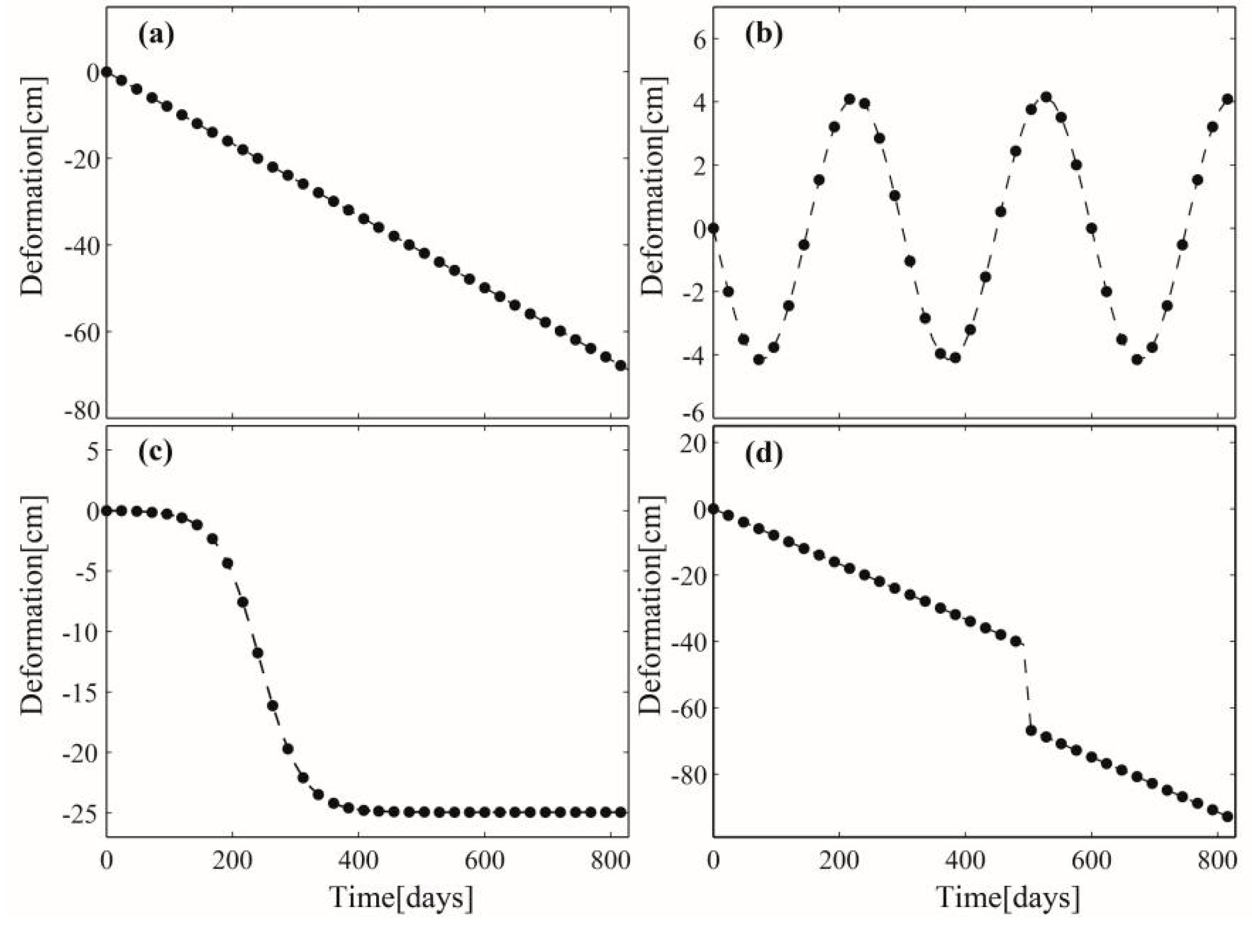
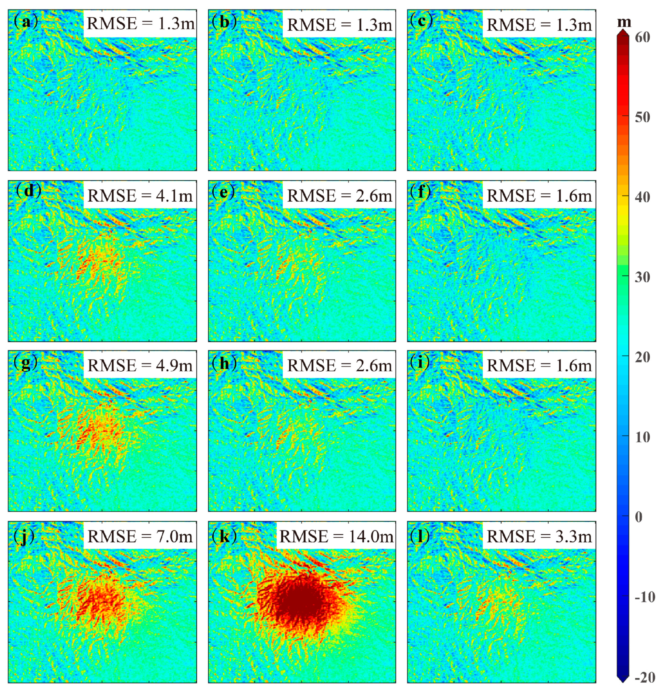
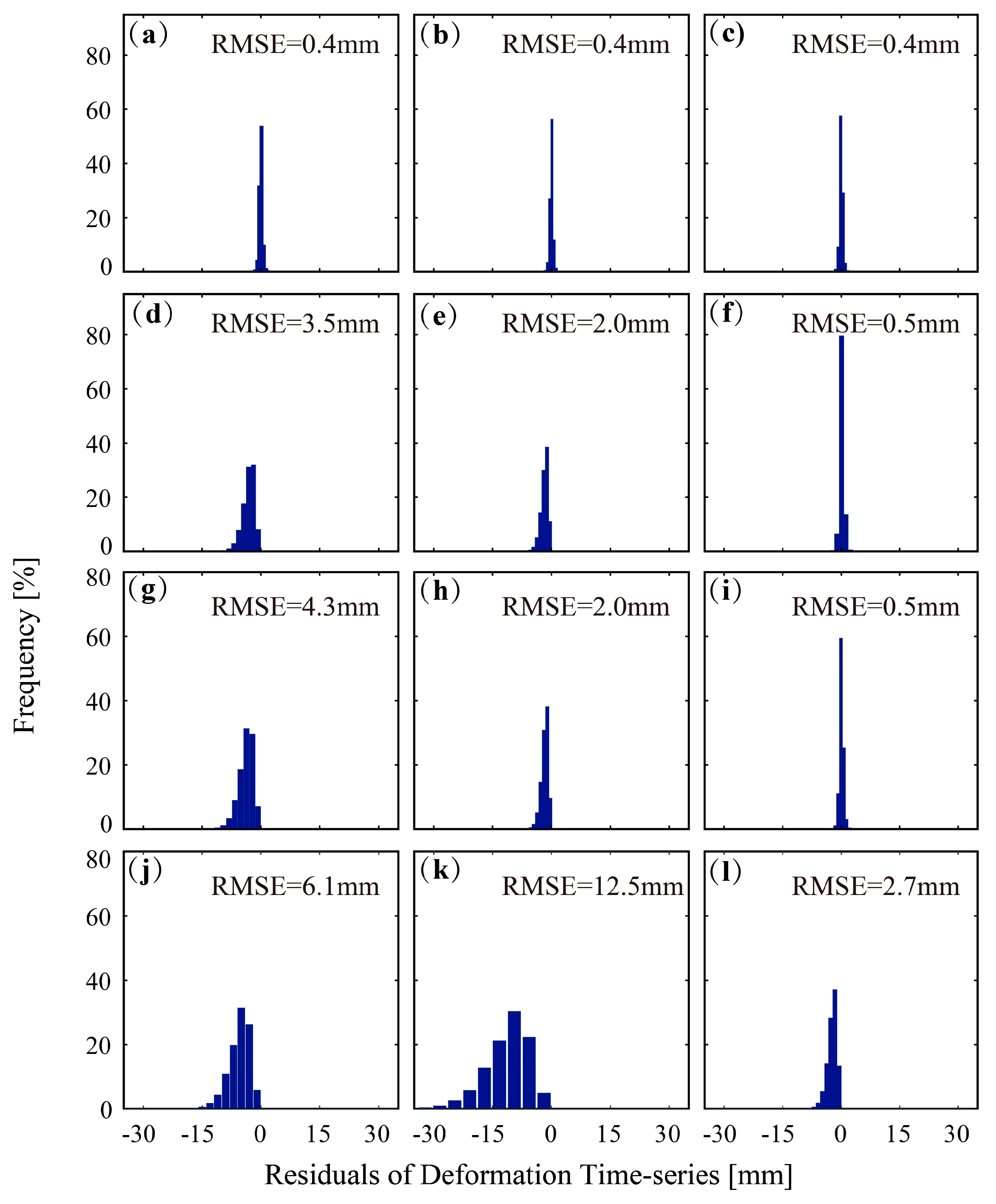
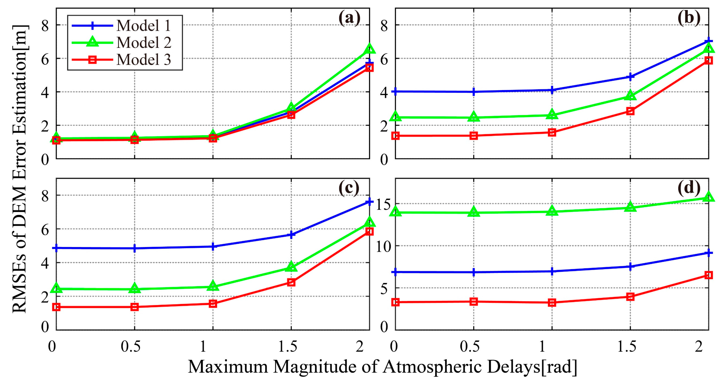
3.1. Simulated Experiments

In the simulation, 159 interferograms were generated from 52 SLCs according to the real spatial–temporal baselines of the Sentinel-1A SAR data acquired over the Pingchuan mining area, Gansu Province, China, which were used in the real data experiment. The spatial pattern of the deformation field (200 × 200 pixels) was simulated based on the fractional volumetric change of the subsurface fluid [42] (see Figure 2). The temporal deformation patterns were simulated by four kinds of functions, i.e., linear, periodic, logistic, and complex functions, and the simulated deformation time series at the central point of Figure 2 are shown in Figure 3. The simulated deformation time series at each point can be obtained by multiplying the pixel value (Figure 2) and the temporal deformation patterns (Figure 3). The DEM error is the difference between Shuttle Radar Topography Mission (SRTM) DEM and TanDEM-X DEM (see Figure 4). The atmospheric delays were simulated using a fractal surface with the fractal dimension being 2.2 and the maximum value being 1.0 rad for each SAR image [43]. The decorrelation noise was modeled as a zero-mean Gaussian random process with the standard deviation σ = ( 1 γ 2 ) / 2 / γ 2 , where γ = e x p ( Δ t / T ) is the coherence simulation based on the temporal baseline Δ t and a time constant T ( T = 60 days in this paper to let γ > 0.5 ) [37]. Figure 5 shows these simulated components of one interferogram.
For comparison, the traditional SBAS-InSAR method with the linear deformation model (Model 1), the traditional SBAS-InSAR method with function group (i.e., Equation (7)) (Model 2), and the proposed method (Model 3) were used to estimate the DEM error and the final deformation time series in the four temporal patterns of deformations. Note that the Model 1 and Model 2 are applied to the whole time series. The accuracy of the estimation is quantitatively described by the root-mean-square error (RMSE), which can be calculated by:
R M S E = i = 1 N U M ( e ^ i e i ) 2 N U M
where e ^ i and e i are the parameter estimation and simulated true value, respectively, and N U M is the number of samples. Note that NUM equals the number of pixels in the calculation of the RMSE of DEM error, and equals the production of the number of pixels and the number of SAR images in the calculation the RMSE of deformation.
As shown in Figure 6, the DEM errors estimated by Models 1 and 2 are seriously affected by deformation signals, which is expected, since the deformation model used by these two methods cannot well describe the deformation evolution. On the contrary, the proposed method can achieve a higher accuracy of DEM error estimation due to the adaptive deformation model and the grouping strategy. For linear deformations (Figure 6a–c), all three methods can obtain very similar DEM error results, since the linear deformation can be well fitted by the linear model, the function group model, and the proposed adaptive deformation model. For periodic (Figure 6d–f) and logistic deformations (Figure 6g–i), the proposed method can obtain more reasonable DEM error results compared to the other two methods. For complex deformations (Figure 6j–l), although it is difficult to fit the deformation evolution with these common functions, the proposed method still performs much better than the other two methods. It should be noted that, for the complex model, the location of the discontinuity concerns the accuracy of the results. If the discontinuity is located in the overlapping area of two adjacent groups, the fitting reliability of both of these groups would be influenced. Otherwise, only one group would be influenced. In real situations, the moment of deformation jump can usually be known before the data processing. In this case, the grouping strategy can be modified based on deformation jump moment to suppress this influence on the result.
Furthermore, the accuracy of the final deformation time series was also investigated, and the residual histograms of the deformation time series with respect to different methods are shown in Figure 7. As can be seen, the accuracy of the deformation time series is consistent with the accuracy of the DEM error estimation, i.e., the proposed method can achieve better deformation results than the other two methods. This indicates that the deformation model involved in the SBAS-InSAR process has a nonnegligible effect on final deformation time series.
For determining the adaptive deformation model, the phase time series without the correction of atmospheric delay were used as the observation. In this case, the existence of atmospheric delay was not conducive to the construction of adaptive deformation model. Therefore, we conducted a series of simulated experiments with the maximum atmospheric delay value ranging from 0.0 to 2.0 rad to investigate the effect of atmospheric delay on the estimation of DEM error. As shown in Figure 8, the RMSEs of the DEM error estimation increase with an increase in the atmospheric delay magnitude for all kinds of deformations and all three methods. Nevertheless, the proposed adaptive deformation model achieved higher accuracy for different magnitudes of atmospheric delay compared to the other two methods, demonstrating the superiority of the proposed adaptive deformation model.

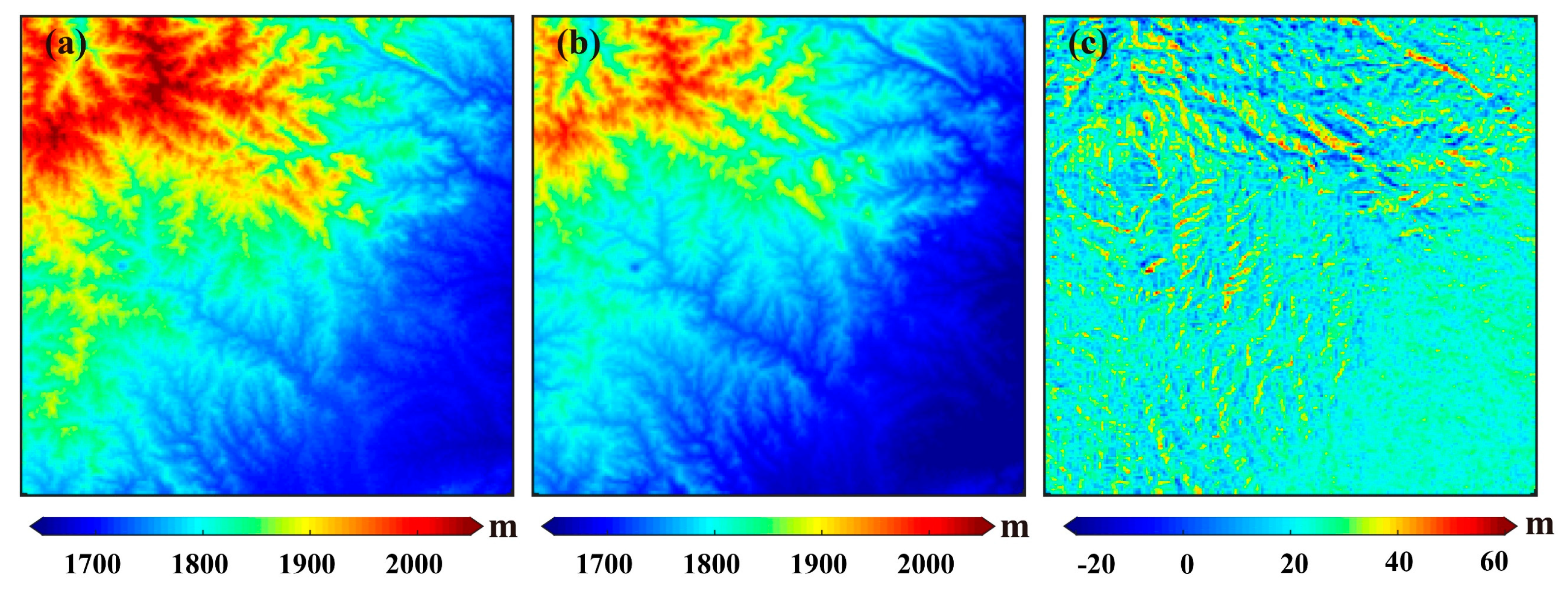
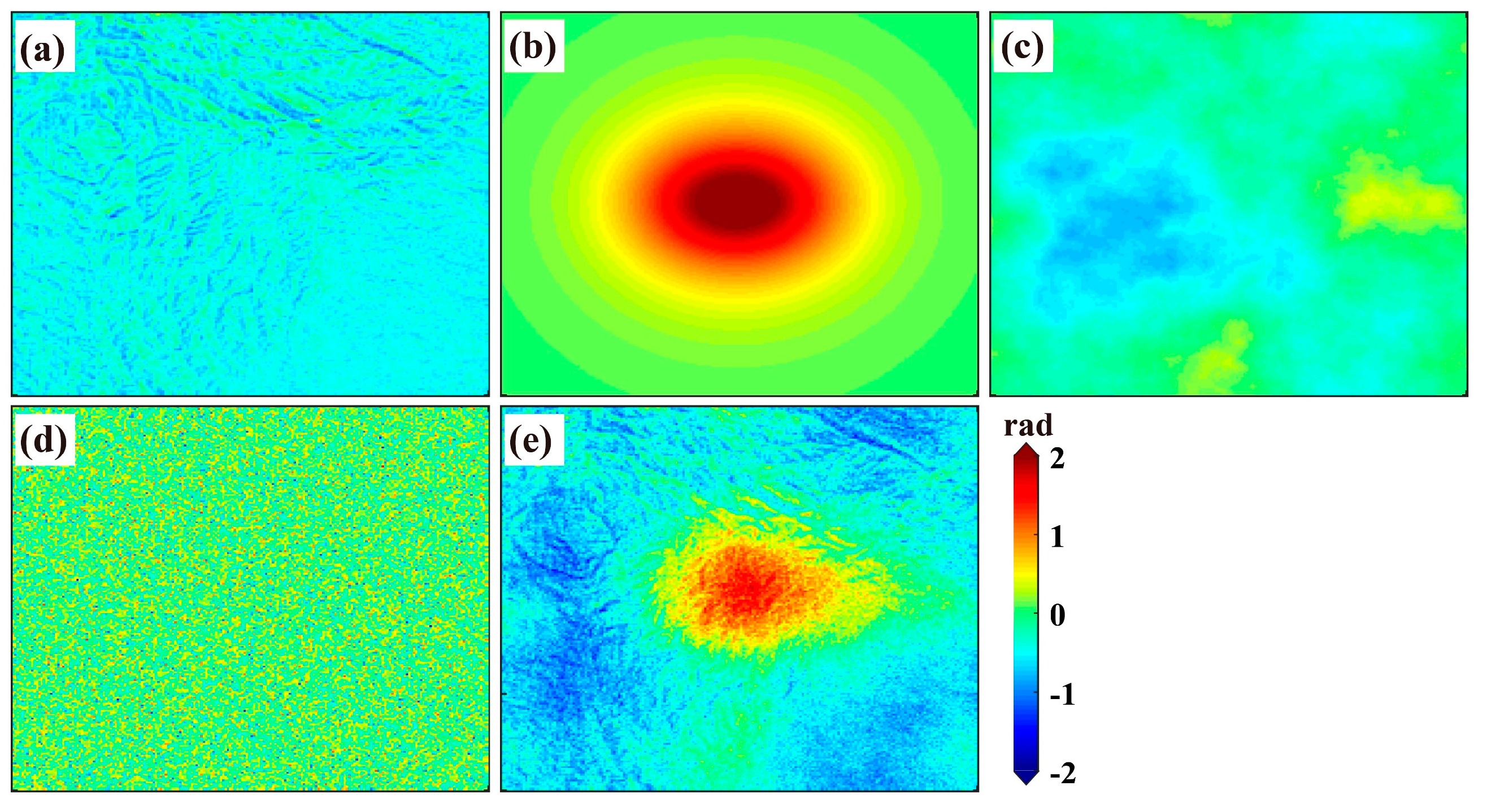
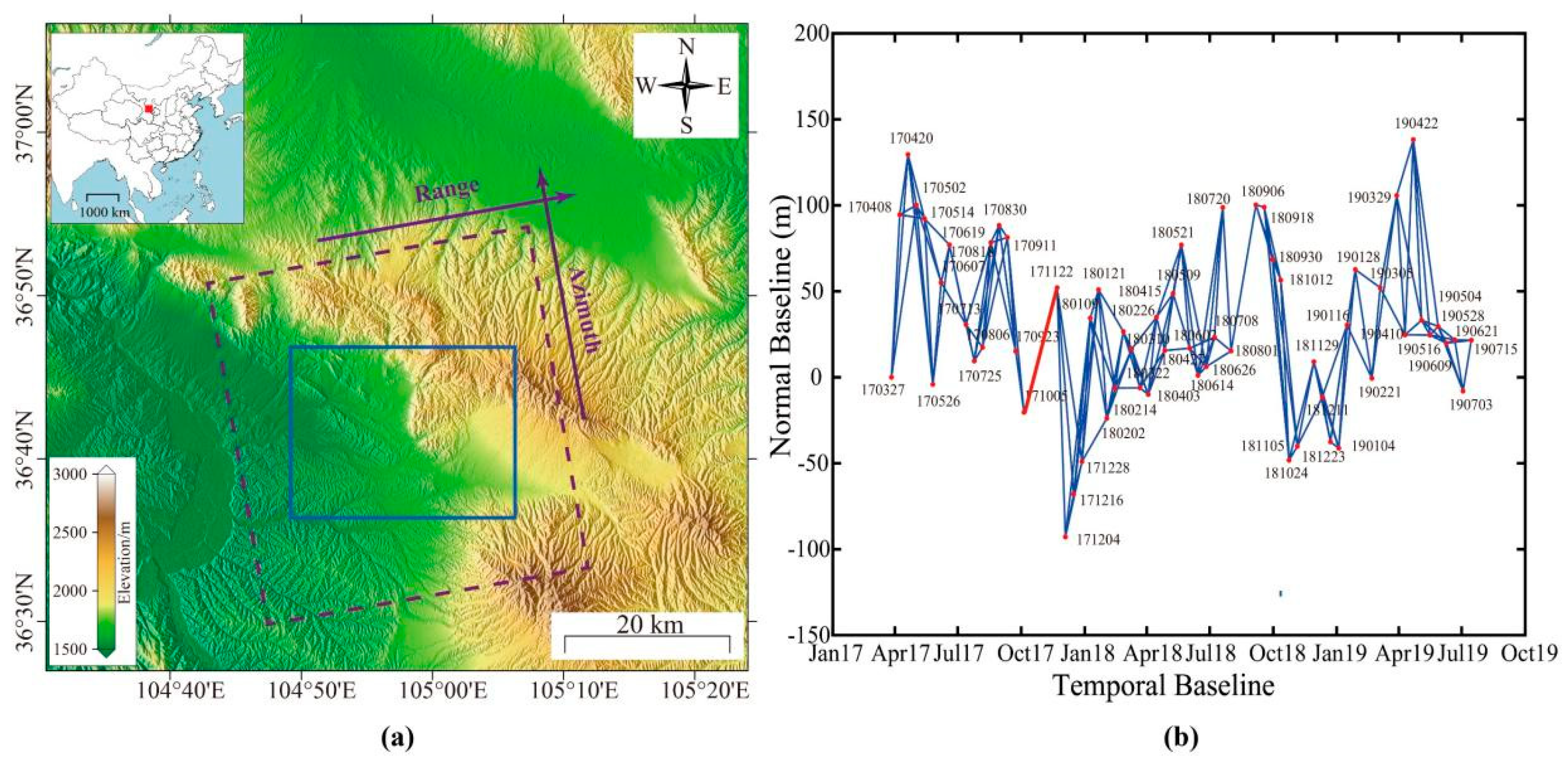
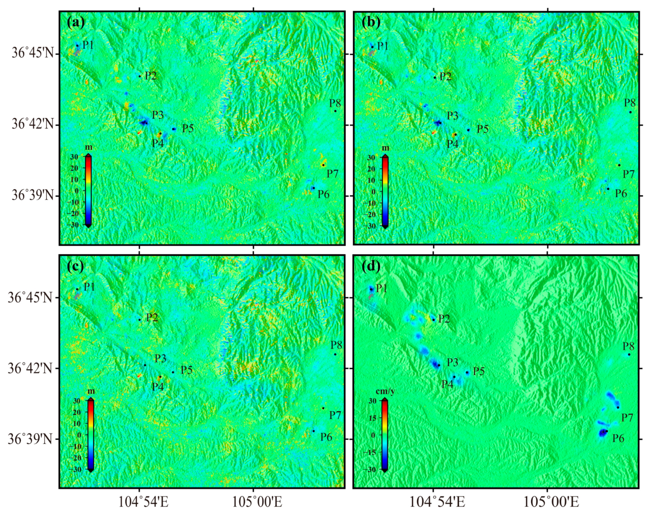
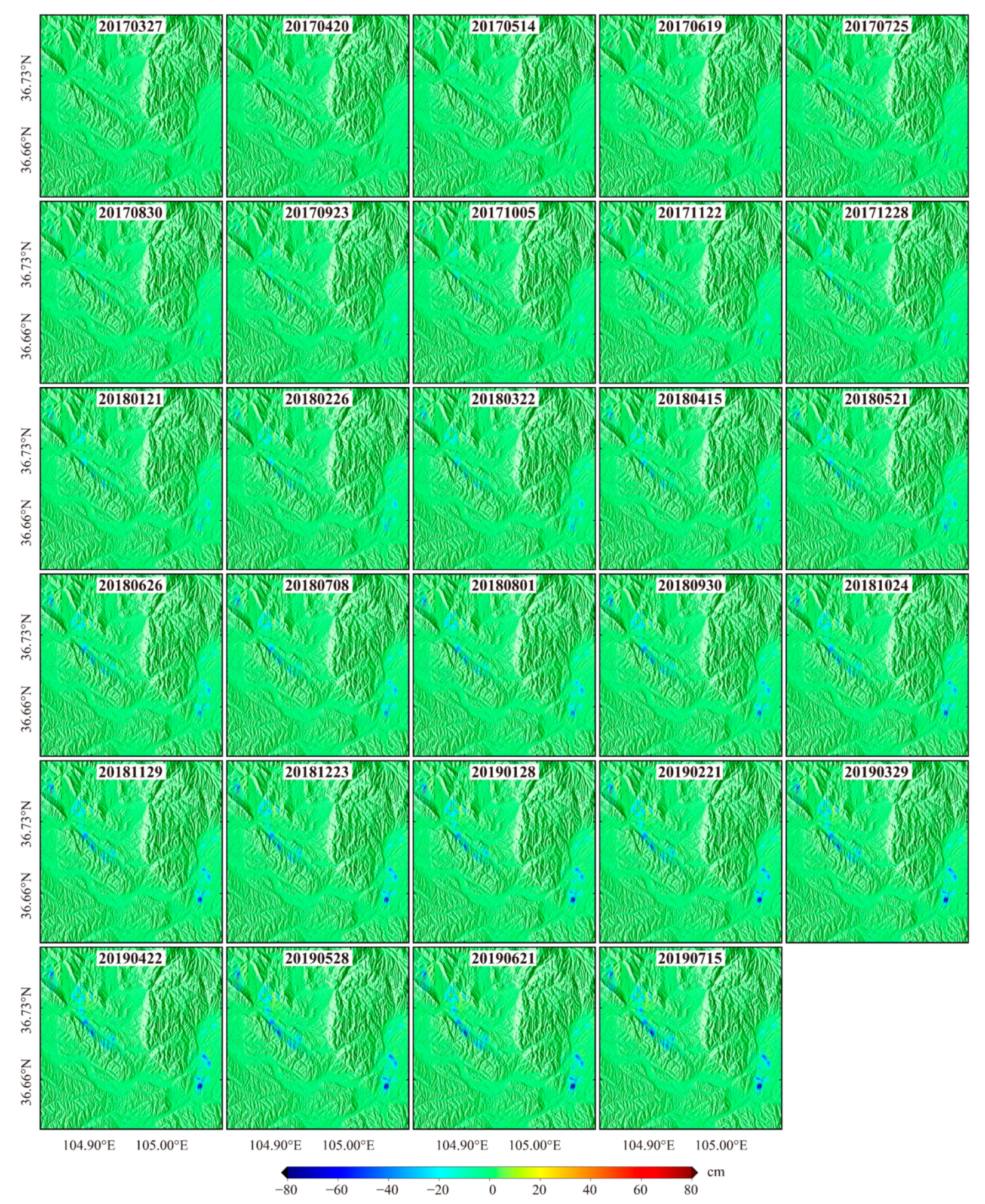
3.2. Real Data Experiments in the Pingchuan Mining Area

The Pingchuan mining area belongs to the Jingyuan coal field, which is one of the important coal bases in Gansu Province, China (see Figure 9). The Pingchuan mining area is rich in coal reserves, and coal mining began in this area as early as the 1970s [44]. With the continuous mining of underground coal, the ground surface suffers serious deformation, which has a negative impact on the safety of people’s lives and property. The SBAS-InSAR method can be used to monitor such deformation, therefore providing a reliable database for policy decisions. However, the classical SBAS-InSAR method is vulnerable to the unreliable a priori deformation model, which is especially important for the case of highly nonlinear deformation time series in the mining area. Therefore, in this paper, the proposed method was employed to obtain more reliable estimations of the DEM error and deformation for the Pingchuan mining area.
Fifty-two Sentinel-1A SAR images were acquired over the Pingchuan mining area from 27 March 2017 to 15 July 2019 (see Figure 9a), and 158 interferograms were generated with the maximum temporal and spatial baselines of 36 days and 200 m, respectively (Figure 9b). To ensure all interferograms belong to a single set, we manually connected the SAR images acquired on 5 October 2017 and 22 November 2017 to generate the 159th interferogram (see the red line in Figure 9b). During the InSAR processing, the topographic phase was removed based on the Shuttle Radar Topography Mission (SRTM) 1 arc-second DEM [45].
Figure 10a–c show the DEM error estimation by the traditional SBAS-InSAR method with the linear deformation model (Model 1), the traditional SBAS-InSAR method with the function group model (Model 2), and the proposed method (Model 3), respectively. Compared to the deformation rate map (Figure 10d), it is easy to see that the spatial pattern of the DEM error estimation by Models 1 and 2 is somewhat similar to the spatial pattern of the deformation rate, indicating that the deformation and the DEM error are not well distinguished in these two methods. On the contrary, the DEM error estimated by Model 3 seems more reasonable and shows less correlation with the deformation. Furthermore, the deformation time series of eight points (i.e., P1–P8 in Figure 10) are presented in Figure 11. The deformations at P1, P3, P5, P6, and P7 show an obvious nonlinear pattern. Compared to Figure 10a,b, it can be found that the DEM error signals at these points are all very large, indicating that these DEM error signals may be caused by the inaccurate deformation models used in Models 1 and 2. As for the points P2, P4, and P8, at which the deformation time series are not as nonlinear as the deformation at P1, P3, P5, P6, and P7, the magnitude of the DEM error estimation is not so correlated with the deformation rate.
The deformation time series at P3 were taken as an example to show the difference between the different methods (see Figure 11b). As can be seen, the differences in the deformation time series obtained by the different methods are much smaller compared to the long-term accumulated deformation. Nevertheless, the deformation varies as much as several millimeters in some moments between the different methods (Figure 11c). This magnitude of deformation cannot be negligible when millimeter-level precision is expected in the monitoring of ground deformation. Figure 12 shows the deformation time series retrieved from the proposed method, in which only one deformation map per month is illustrated. The maximum cumulate deformation along the LOS direction, which occurred around the vicinity of P6, was approximately −88.5 cm, where the negative value indicates the ground moving away from the satellite.

4. Discussion

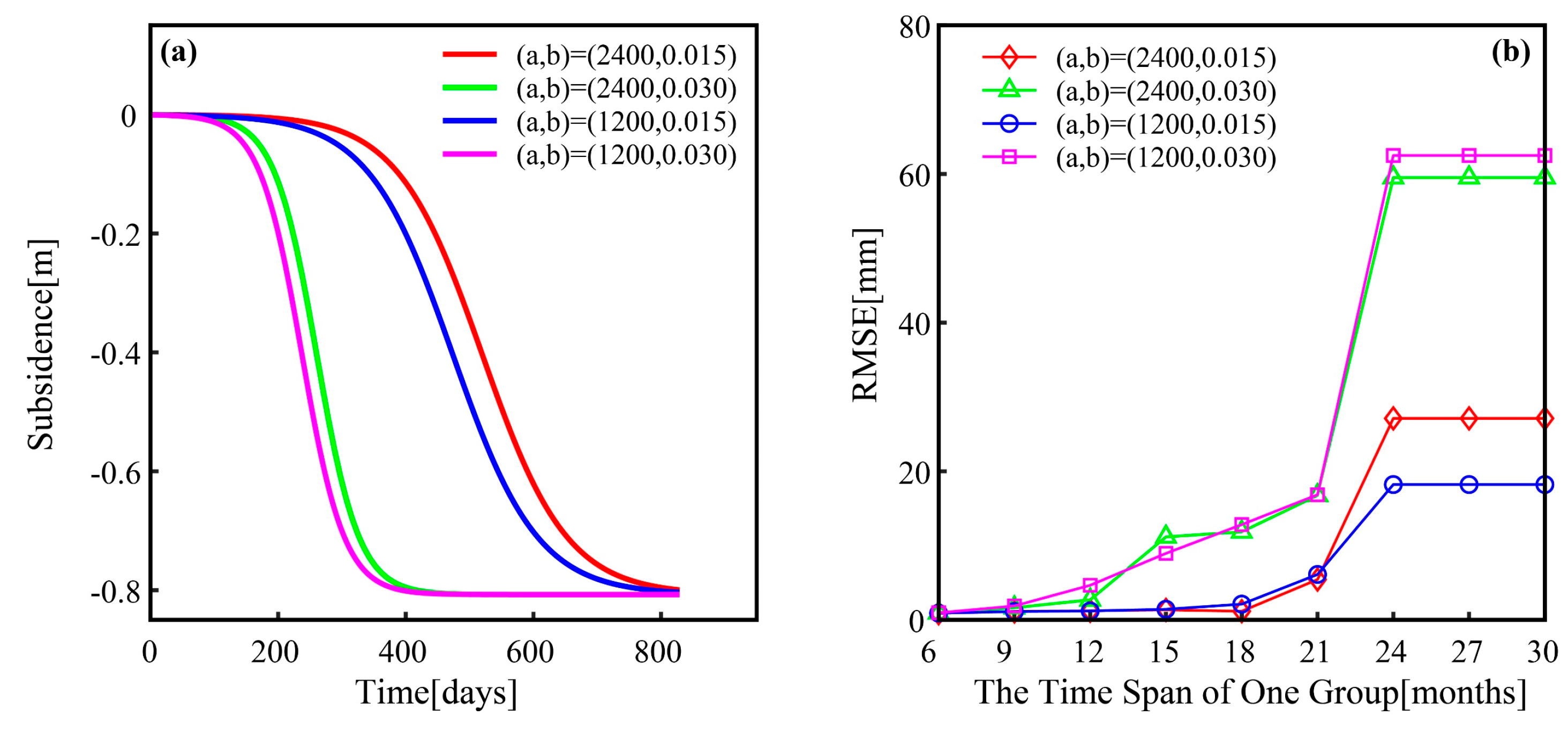
4.1. Determining the Time Span of Each Group in the Grouping Process

Since one of the key steps of the proposed method is to group observations, we verified the rationality of this grouping strategy based on the simulation of four kinds of mining subsidence deformations (see Figure 13a) and simultaneously determined the time span of each group in the grouping process. The mining subsidence was simulated based on the logistic function [46]:
d ( t ) = d 0 1 + a exp ( b t )
where d ( t ) denotes the cumulative subsidence at time t, d 0 represents the maximum subsidence value,   a and b are the shape parameters of the logistic function. Here, d 0 = 0.8   m , and the values of (a, b) are (2400, 0.015), (2400, 0.030), (1200, 0.015), and (1200, 0.030), respectively. Similar to the Sentinel-1 SAR satellite, we simulated 70 acquisitions with a 12-day sampling interval across two and half years, and the time span of the observations in each group varied from six months to two and a half years. As shown in Figure 13b, the RMSEs of the fitting deformations by grouping increase with the increase in the observation time span in a group for the four kinds of deformations, indicating that the shorter the time span in each group (i.e., the more groups), the higher the fitting accuracy of the deformation model. However, the short time span decreases the number of independent time series observations, and would increase the risk of model overfitting. Therefore, a one-year time span in a group was preferred in this paper to obtain a tradeoff between the accuracy of deformation and the possibility of overfitting, and this grouping strategy was adopted in both the simulated and the real data experiments.

4.2. Decreasing Correlation between the Deformation Rate and the DEM Error Estimation Based on the Proposed Method

In order to further demonstrate the superiority of the proposed method, we calculated the correlation coefficients between the deformation rate and the DEM error estimations of the different methods at the vicinity of P1–P8 (see Table 1).
As shown in Table 1, the DEM error estimations at the points whose deformation patterns are roughly linear (P2, P4, and P8) show low correlation with the deformation rate for all three deformation models. However, at those points, with obviously nonlinear deformations (P1, P3, P5, P6, and P7), the DEM error estimation shows a strong correlation with the deformation rate for Model 1, with correlation coefficients greater than 0.5; this correlation is decreased for Model 2 compared to Model 1, since the function group in Model 2 can better fit nonlinear deformation than the linear function in Model 1. For Model 3, the DEM error estimations show the slightest correlation with the deformation rate compared to the results of Models 1 and 2, indicating that the proposed method can construct a more reliable deformation model and then obtain more reasonable DEM error estimation.

5. Conclusions

DEM error is one of the components in the InSAR phase and is usually estimated with the help of an a priori deformation model. However, since the temporal deformation evolution is usually unknown, it is difficult to use a definite function to fit temporal deformation, which is not conducive to the estimation of DEM error and deformation time series. In this paper, we proposed a method to construct adaptive deformation models in the SBAS-InSAR framework based on the hypothesis testing theory. In particular, the phase time series were first divided into several groups with overlapping regions. In each group, we used a set of predefined functions to fit the deformation time series. In order to prevent the occurrence of overfitting, the hypothesis testing theory was introduced to adaptively select the optimal deformation model from the predefined functions, after which the parameters of the adaptive deformation models in each group and the DEM error were simultaneously solved by a least-squares method. Both simulated and real data experiments in the Pingchuan mining area were conducted. The results show that the proposed method can effectively improve the accuracy of DEM error estimation and can also benefit the accuracy of deformation time series.
It should be noted that the proposed method can also be embedded in other state-of-the-art TS-InSAR techniques to construct more suitable deformation models and to obtain more reliable DEM error, as well as deformation. Moreover, the proposed method can be further improved by adjusting the original deformation model functions (i.e., Equation (7)) based on a priori information about the deformation evolution process. For example, a time-related jump function (e.g., the Heaviside function [47]) can be used if there is an abrupt event.

Author Contributions

Conceptualization, J.H., Q.G., and J.L.; methodology, J.H. and J.L.; software, J.H.; validation, J.H., Q.G., and J.L.; formal analysis, Q.G. and J.H.; investigation, W.Y.; resources, Z.D. and L.H.; data curation, J.H. and Q.G.; writing—original draft preparation, J.H. and Q.G.; writing—review and editing, all authors.; supervision, J.H.; funding acquisition, J.H., Z.D., and L.H. All authors have read and agreed to the published version of the manuscript.

Funding

This research was funded by the National Natural Science Foundation of China (grant number 42030112), the National Key Basic Research and Development Program of China (grant number 2018YFC1505101), the Hunan Natural Science Foundation (grant number 2020JJ2043), the Special Fund for the Construction of Innovative Provinces in Hunan (grant number 2019GK5006), the Project of Innovation-Driven Plan of Central South University (grant number 2019CX007), and the Fundamental Research Funds for the Central Universities of Central South University (grant numbers 2019zzts640 and 2020zzts647).

Data Availability Statement

The data used to support the findings of this study are available from the corresponding author upon request.

Acknowledgments

The Sentinel-1 SAR datasets were freely obtained from the official website of European Space Agency. The SRTM and TanDEM-X DEM data were freely downloaded from USGS and DLR, respectively. The authors thank two anonymous reviewers for their helpful comments, which great improve the quality of the paper.

Conflicts of Interest

The authors declare no conflict of interest.

References

  1. Ng, A.H.-M.; Ge, L.L.; Zhang, K.; Chang, H.C.; Li, X.J.; Chris, R.; Omura, M. Deformation mapping in three dimensions for underground mining using InSAR–Southern highland coalfield in New South Wales, Australia. Int. J. Remote Sens. 2011, 32, 7227–7256. [Google Scholar] [CrossRef]
  2. Yang, Z.F.; Li, Z.W.; Zhu, J.J.; Wang, Y.D.; Wu, L.X. Use of SAR/InSAR in Mining Deformation Monitoring, Parameter Inversion, and Forward Predictions: A Review. IEEE Geosci. Remote Sens. Mag. 2020, 8, 71–90. [Google Scholar] [CrossRef]
  3. Ng, A.H.-M.; Ge, L.L.; Du, Z.Y.; Wang, S.R.; Ma, C. Satellite radar interferometry for monitoring subsidence induced by longwall mining activity using Radarsat-2, Sentinel-1 and ALOS-2 data. Int. J. Appl. Earth Obs. Geoinf. 2017, 61, 92–103. [Google Scholar] [CrossRef]
  4. Singleton, A.; Li, Z.; Hoey, T.; Muller, J.P. Evaluating sub-pixel offset techniques as an alternative to D-InSAR for monitoring episodic landslide movements in vegetated terrain. Remote Sens. Environ. 2014, 147, 133–144. [Google Scholar] [CrossRef] [Green Version]
  5. Sun, Q.; Zhang, L.; Ding, X.L.; Hu, J.; Li, Z.W.; Zhu, J.J. Slope deformation prior to Zhouqu, China landslide from InSAR time series analysis. Remote Sens. Environ. 2015, 156, 45–57. [Google Scholar] [CrossRef]
  6. Cigna, F.; Tapete, D. Sentinel-1 BigData Processing with P-SBAS InSAR in the Geohazards Exploitation Platform: An Experiment on Coastal Land Subsidence and Landslides in Italy. Remote Sens. 2021, 13, 885. [Google Scholar] [CrossRef]
  7. Hu, J.; Li, Z.W.; Ding, X.L.; Zhu, J.J.; Sun, Q. Derivation of 3-D coseismic surface displacement fields for the 2011 Mw 9.0 Tohoku-Oki earthquake from InSAR and GPS measurements. Geophys. J. Int. 2012, 192, 573–585. [Google Scholar] [CrossRef] [Green Version]
  8. Liu, J.H.; Hu, J.; Xu, W.B.; Li, Z.W.; Zhu, J.J.; Ding, X.L.; Zhang, L. Complete Three-Dimensional Coseismic Deformation Field of the 2016 Central Tottori Earthquake by Integrating Left- and Right- Looking InSAR Observations With the Improved SM-VCE Method. J. Geophys. Res. Solid Earth 2019, 124, 12099–12115. [Google Scholar] [CrossRef] [Green Version]
  9. Hu, J.; Wang, Q.J.; Li, Z.W.; Xie, R.A.; Zhang, X.Q.; Sun, Q. Retrieving three-dimensional coseismic displacements of the 2008 Gaize, Tibet earthquake from multi-path interferometric phase analysis. Nat. Hazards 2014, 73, 1311–1322. [Google Scholar] [CrossRef]
  10. Liu, J.H.; Hu, J.; Li, Z.W.; Zhu, J.J.; Sun, Q.; Gan, J. A Method for Measuring 3-D Surface Deformations With InSAR Based on Strain Model and Variance Component Estimation. IEEE Trans. Geosci. Remote Sens. 2018, 56, 239–250. [Google Scholar] [CrossRef]
  11. Solaro, G.; Acocella, V.; Pepe, S.; Ruch, J.; Neri, M.; Sansosti, E. Anatomy of an unstable volcano from InSAR: Multiple processes affecting flank instability at Mt. Etna, 1994–2008. J. Geophys. Res. Solid Earth 2010. [Google Scholar] [CrossRef]
  12. Richter, N.; Froger, J.L. The role of Interferometric Synthetic Aperture Radar in Detecting, Mapping, Monitoring, and Modelling the Volcanic Activity of Piton de la Fournaise, La Réunion: A Review. Remote Sens. 2020, 12, 1019. [Google Scholar] [CrossRef] [Green Version]
  13. Ferretti, A.; Prati, C. Nonlinear subsidence rate estimation using permanent scatterers in differential SAR interferometry. IEEE Trans. Geosci. Remote Sens. 2000, 38, 2202–2212. [Google Scholar] [CrossRef] [Green Version]
  14. Ferretti, A.; Prati, C.; Rocca, F. Permanent scatterers in SAR interferometry. IEEE Trans. Geosci. Remote Sens. 2001, 39, 8–20. [Google Scholar] [CrossRef]
  15. Berardino, P.; Fornaro, G.; Lanari, R.; Sansosti, E. A new algorithm for surface deformation monitoring based on small baseline differential SAR interferograms. IEEE Trans. Geosci. Remote Sens. 2002, 40, 2375–2383. [Google Scholar] [CrossRef] [Green Version]
  16. Ferretti, A.; Fumagalli, A.; Novali, F.; Prati, C.; Rocca, F.; Rucci, A. A New Algorithm for Processing Interferometric Data-Stacks: SqueeSAR. IEEE Trans. Geosci. Remote Sens. 2011, 49, 3460–3470. [Google Scholar] [CrossRef]
  17. Xue, F.Y.; Lv, X.L.; Dou, F.J.; Ye, Y. A Review of Time-Series Interferometric SAR Techniques: A Tutorial for Surface Deformation Analysis. IEEE Geosci. Remote Sens. Mag. 2020, 8, 22–42. [Google Scholar] [CrossRef]
  18. Hanssen, R.F. Radar Interferometry Data Interpretation and Error Analysis; Springer Science & Business Media: Berlin, Germany, 2001. [Google Scholar]
  19. Zebker, H.A.; Rosen, P.A.; Hensley, S. Atmospheric effects in interferometric synthetic aperture radar surface deformation and topographic maps. J. Geophys. Res. Solid Earth 1997, 102, 7547–7563. [Google Scholar] [CrossRef]
  20. Li, Z.W.; Xu, W.B.; Feng, G.C.; Hu, J.; Wang, C.C.; Ding, X.L.; Zhu, J.J. Correcting atmospheric effects on InSAR with MERIS water vapour data and elevation-dependent interpolation model. Geophys. J. Int. 2012, 189, 898–910. [Google Scholar] [CrossRef] [Green Version]
  21. Mateus, P.; Nico, G.; Catalao, J. Uncertainty Assessment of the Estimated Atmospheric Delay Obtained by a Numerical Weather Model (NMW). IEEE Trans. Geosci. Remote Sens. 2015, 53, 6710–6717. [Google Scholar] [CrossRef]
  22. Li, Z.H.; Fielding, E.J.; Cross, P.; Preusker, R. Advanced InSAR atmospheric correction: MERIS/MODIS combination and stacked water vapour models. Int. J. Remote Sens. 2009, 30, 3343–3363. [Google Scholar] [CrossRef]
  23. Xu, B.; Li, Z.W.; Wang, Q.J.; Jiang, M. A Refined Strategy for Removing Composite Errors of SAR Interferogram. IEEE Geosci. Remote Sens. Lett. 2013, 11, 143–147. [Google Scholar] [CrossRef]
  24. Hu, J.; Liu, J.H.; Li, Z.W.; Zhu, J.J.; Wu, L.X.; Sun, Q.; Wu, W.Q. Estimating three-dimensional coseismic deformations with the SM-VCE method based on heterogeneous SAR observations: Selection of homogeneous points and analysis of observation combinations. Remote Sens. Environ. 2021, 255. [Google Scholar] [CrossRef]
  25. Du, Y.N.; Zhang, L.; Feng, G.C.; Lu, Z.; Sun, Q. On the Accuracy of Topographic Residuals Retrieved by MTInSAR. IEEE Trans. Geosci. Remote Sens. 2017, 55, 1053–1065. [Google Scholar] [CrossRef]
  26. Zheng, W.J.; Hu, J.; Liu, J.H.; Sun, Q.; Li, Z.W.; Zhu, J.J.; Wu, L.X. Mapping Complete Three-Dimensional Ice Velocities by Integrating Multi-Baseline and Multi-Aperture InSAR Measurements: A Case Study of the Grove Mountains Area, East Antarctic. Remote Sens. 2021, 13, 643. [Google Scholar] [CrossRef]
  27. Agram, P.S.; Simons, M. A noise model for InSAR time series. J. Geophys. Res. Solid Earth 2015. [Google Scholar] [CrossRef]
  28. Sun, Q.; Zhang, L.; Hu, J.; Ding, X.L.; Li, Z.W.; Zhu, J.J. Characterizing sudden geo-hazards in mountainous areas by D-InSAR with an enhancement of topographic error correction. Nat. Hazards 2014, 75, 2343–2356. [Google Scholar] [CrossRef]
  29. Samsonov, S. Topographic Correction for ALOS PALSAR Interferometry. IEEE Trans. Geosci. Remote Sens. 2010, 48, 3020–3027. [Google Scholar] [CrossRef]
  30. Fattahi, H.; Amelung, F. DEM Error Correction in InSAR Time Series. IEEE Trans. Geosci. Remote Sens. 2013, 51, 4249–4259. [Google Scholar] [CrossRef]
  31. Shanker, P.; Zebker, H. Persistent scatterer selection using maximum likelihood estimation. Geophys. Res. Lett. 2007, 34, 315–324. [Google Scholar] [CrossRef]
  32. Zhang, L.; Lu, Z.; Ding, X.L.; Jung, H.S.; Feng, G.C.; Lee, C.W. Mapping ground surface deformation using temporarily coherent point SAR interferometry: Application to Los Angeles Basin. Remote Sens. Environ. 2012, 117, 429–439. [Google Scholar] [CrossRef]
  33. Li, S.S.; Li, Z.W.; Hu, J.; Sun, Q.; Yu, X.Y. Investigation of the seasonal oscillation of the permafrost over Qinghai-Tibet Plateau with SBAS-InSAR algorithm. Chin. J. Geophys. 2013, 56, 1476–1486. [Google Scholar] [CrossRef]
  34. Hetland, E.A.; Musé, P.; Simons, M.; Lin, Y.N.; Agram, P.S.; Dicaprio, C.J. Multiscale InSAR Time Series (MInTS) analysis of surface deformation. J. Geophys. Res. Solid Earth 2012, 117. [Google Scholar] [CrossRef] [Green Version]
  35. Liang, H.Y.; Zhang, L.; Lu, Z.; Li, X. Nonparametric Estimation of DEM Error in Multitemporal InSAR. IEEE Trans. Geosci. Remote Sens. 2019, 57, 10004–10014. [Google Scholar] [CrossRef]
  36. Hyvarinen, A.; Oja, E. Independent Component Analysis: Algorithms and Applications. Neural Netw. 2000, 13, 411–430. [Google Scholar] [CrossRef] [Green Version]
  37. Wang, J.L.; Deng, Y.K.; Wang, R.; Ma, P.F.; Lin, H. A Small-Baseline InSAR Inversion Algorithm Combining a Smoothing Constraint and L1-Norm Minimization. IEEE Geosci. Remote Sens. Lett. 2019, 1–5. [Google Scholar] [CrossRef]
  38. Tao, B.Z. Non-linear Adjustment of Deformation Inversion Model. Geomat. Inf. Sci. Wuhan Univ. 2001, 26, 504–508. [Google Scholar] [CrossRef]
  39. Olive, D.J. Multiple Linear Regression. In Linear Regression; Springer International Publishing: Cham, Switzerland, 2017; pp. 17–83. [Google Scholar]
  40. Van Leijen, F.J.; Hanssen, R.F. Persistent scatterer density improvement using adaptive deformation models. In Proceedings of the IEEE International Geoscience and Remote Sensing Symposium, Barcelona, Spain, 23–27 July 2007; pp. 2102–2105. [Google Scholar]
  41. Lanari, R.; Mora, O.; Manunta, M.; Mallorquí, J.; Sansosti, E. A small-baseline approach for investigating deformations on full-resolution differential SAR interferograms. IEEE Trans. Geosci. Remote Sens. 2004, 42, 1377–1386. [Google Scholar] [CrossRef]
  42. Hu, J.; Ding, X.L.; Zhang, L.; Sun, Q.; Li, Z.W.; Zhu, J.J.; Lu, Z. Estimation of 3-D Surface Displacement Based on InSAR and Deformation Modeling. IEEE Trans. Geosci. Remote Sens. 2017, 55, 2007–2016. [Google Scholar] [CrossRef]
  43. Kampes, B. Radar Interferometry: Persistent Scatterer Technique; Springer Netherlands: Amsterdam, The Netherlands, 2006. [Google Scholar]
  44. Li, J.H.; Tan, Z.W.; Guan, B.G. A Study on Coal Hosting Features and Prospecting Orientation in Peripheral Baojishan and Honghui Mine Areas, Jingyuan Coalfield. Coal Geol. China 2012, 24, 7–10. [Google Scholar] [CrossRef]
  45. Werner, M. Shuttle Radar Topography Mission (SRTM) Mission Overview. Frequenz 2001, 55, 75–79. [Google Scholar] [CrossRef]
  46. Yang, Z.F.; Yi, H.W.; Zhu, J.J.; Li, Z.W.; Liu, Q. Spatio-temporal evolution law analysis of whole mining subsidence basin based on InSAR-derived time-series deformation. Chin. J. Nonferrous Met. 2016, 26, 1515–1522. [Google Scholar]
  47. Dalaison, M.; Jolivet, R. A Kalman Filter Time Series Analysis method for InSAR. J. Geophys. Res. Solid Earth 2020, 125. [Google Scholar] [CrossRef]
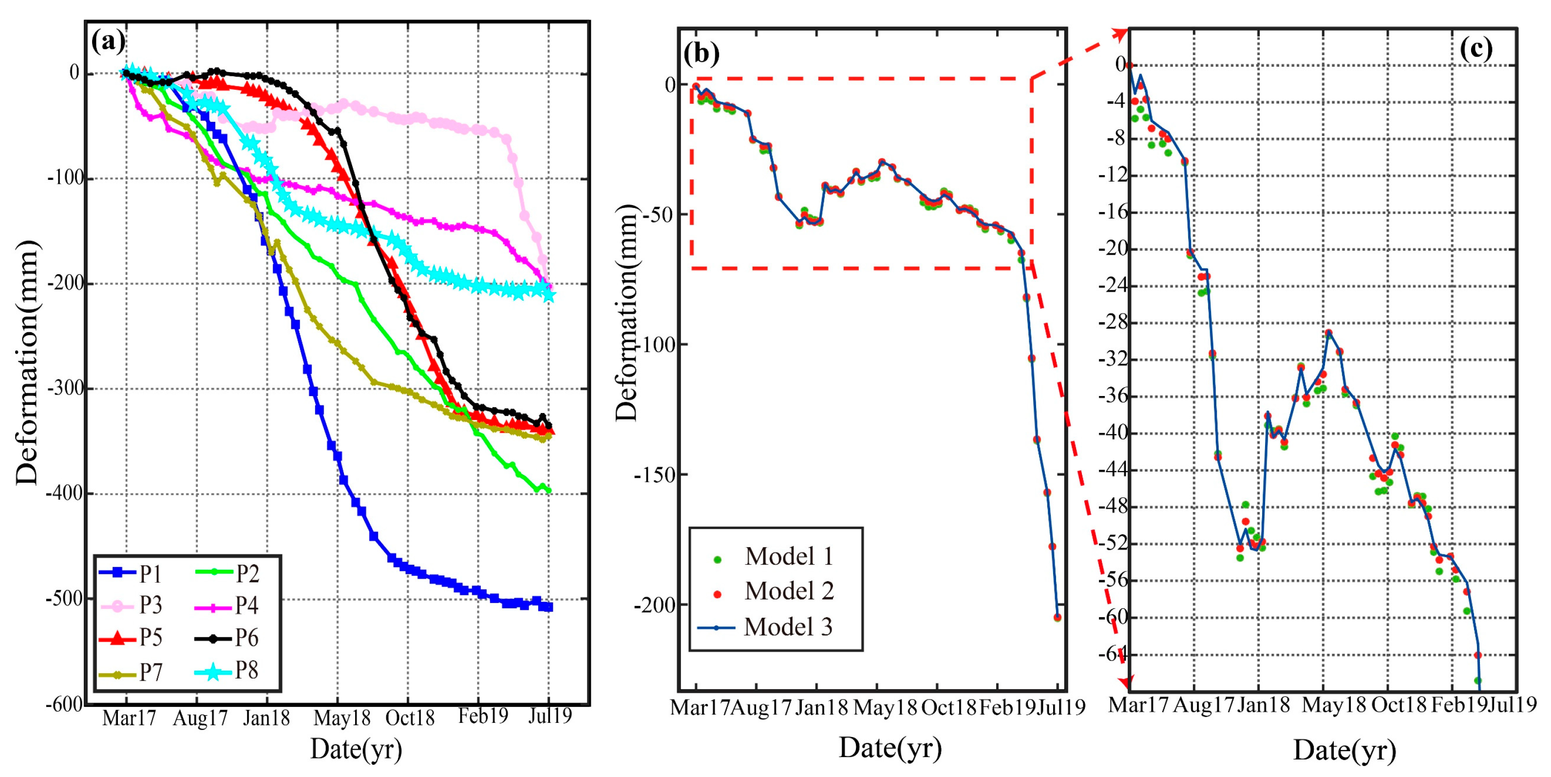
Figure 1. Flow chart of the proposed method.
Remotesensing 13 02006 g001
Figure 2. The spatial deformation pattern.
Remotesensing 13 02006 g002
Figure 3. The temporal deformation patterns: (a) linear; (b) periodic; (c) logistic; (d) complex.
Remotesensing 13 02006 g003
Figure 4. (a) Shuttle Radar Topography Mission (SRTM) DEM; (b) TanDEM-X DEM; (c) the difference between (a,b).
Remotesensing 13 02006 g004
Figure 5. (a) The DEM error-related phase, (b) deformation, (c) atmospheric delay, (d) decorrelation noise, and (e) final interferogram of one simulated interferogram with a perpendicular baseline of 128 m and a temporal baseline of 36 days.
Remotesensing 13 02006 g005
Figure 6. Estimation of the DEM error by (left) the traditional SBAS with the linear deformation model (Model 1), (center) the traditional SBAS with a function group (Model 2), and (right) the proposed method (Model 3). (ac) Linear deformation; (eh) periodic deformation; (gi) logistic deformation; (jl) complex deformation.
Remotesensing 13 02006 g006
Figure 7. Residual histograms between the simulation and estimation of deformation time series by (left) the traditional SBAS-InSAR method with the linear deformation model, (center) the traditional SBAS-InSAR method with a function group, and (right) the proposed method. (ac) Linear deformation; (eh) periodic deformation; (gi) logistic deformation; (jl) complex deformation.
Remotesensing 13 02006 g007
Figure 8. RMSEs of the DEM error estimation for different kinds of temporal deformations and different methods under various magnitudes of maximum atmospheric delay. (a) Linear deformation; (b) periodic deformation; (c) logistic deformation; (d) complex deformation.
Remotesensing 13 02006 g008
Figure 9. (a) Shaded relief map of the study area. The purple dashed rectangle is the area covered by the ascending Sentinel-1A images (Track 55, Frame 117). The blue solid box is the scope of Figure 10. The insert map shows the location of the study area in China. (b) Distribution of spatial–temporal baselines for the selected interferograms. The dots and lines represent the SAR acquisitons and interferometric pairs, respectively. The red line is the manually selected interferogram whose baseline excedes the predifined threshold.
Remotesensing 13 02006 g009
Figure 10. DEM error estimation by (a) the traditional SBAS-InSAR method with the linear deformation model, (b) the traditional SBAS-InSAR method with a function group, and (c) the proposed method. (d) Deformation rate along the line-of-sight (LOS) direction estimated by the proposed method. The negative value in (d) indicates the ground moving away from the satellite. P1–P8 are the selected points.
Remotesensing 13 02006 g010
Figure 11. (a) Deformation time series along the LOS direction at the selected points P1–P8. The negative value indicates the ground moving away from the satellite. (b) Deformation time series at P3 derived by different methods, and the details in the dashed red rectangle are shown in (c).
Remotesensing 13 02006 g011
Figure 12. Time series deformation over the study area.
Remotesensing 13 02006 g012
Figure 13. (a) Four kinds of mining subsidence deformation. (b) The fitting deformation accuracy for the different time spans of one group under the four kinds of deformation.
Remotesensing 13 02006 g013
Table 1. The correlation coefficients between the deformation rate and the DEM error estimations of the different methods at the vicinity of P1–P8.
PointsModel 1Model 2Model 3
P10.660.620.13
P20.150.140.14
P30.730.600.24
P4−0.01−0.02−0.01
P50.690.650.23
P60.540.350.14
P7−0.510.390.18
P80.150.150.13
Publisher’s Note: MDPI stays neutral with regard to jurisdictional claims in published maps and institutional affiliations.

