1. Introduction
In recent years, many emerging applications including, but not limited to, autonomous vehicles, unmanned delivery, and urban surveying have been applied in large-scale outdoor environments and rely on robust and high-precision positioning techniques. Compared with traditional applications, these innovative outdoor applications raise the bar for the performance of positioning concomitantly, which can be concluded as follows [
1]: (1) more diversified working environments, not only in open areas, but also in GNSS-challenged areas such as urban canyons; (2) higher demand in positioning precision, normally at a decimeter or even centimeter level; (3) higher demand in continuity and stability.
So far, several types of sensors have been employed for positioning and navigation purposes, but when used in a stand-alone mode, none can be regarded as omnipotent when facing the above-mentioned requirements. As the most used outdoor positioning technique means, the Global Navigation Satellite System (GNSS) can provide absolute positioning results in the global frame. Based on GNSS, a technology named Real-Time Kinematic (RTK) can further obtain centimeter-level positioning accuracy by using double-differenced carrier phase measurements and performs well in open areas. However, GNSS cannot be used for indoor environments, and even in outdoor GNSS-challenged environments like urban areas, due to partial blockages, the challenges of low satellite availability, the poor geometric distribution, and the strong multipath effect arising, this lead to the deterioration of RTK performance, or specifically, RTK fixing. By contrast, environment-feature-based sensors represented by a Visual System (VS) and Light Detection and Ranging (LiDAR) can achieve a better performance in complicated environments with abundant features, but become worse in open areas. As a kind of dead-reckoning sensor, the Inertial Navigation System (INS) is popular for its short-term high precision and applicability in any environment, but on-going calibration is requisite or else errors will accumulate over time, causing a rapid drift. The characteristics of the aforementioned sensors can complement each other in terms of their working modes and applicable environments. Therefore, as a matter of course, the fusion of combining these sensors has become the only acceptable solution to the problem of robust high-precision positioning in diversified environments.
As a typical application of this type, state-of-the-art autonomous driving systems are generally equipped with a variety of sensors, including GNSS, INS, VS, multiple LiDARs, etc., and a prebuilt LiDAR global map is also used for providing global positions in place of RTK in tough environments, which comes at the cost of cumbersome preparatory work and large storage [
2,
3,
4,
5,
6]. However, this solution is not suitable for all applications. For applications like unmanned delivery, urban surveying, emergency rescue, and unmanned ports, owing to factors such as mapping preliminary burdens and unexplored or changing environments, such prior-map-based schemes may not be that welcome or even totally inapplicable. For these applications, prebuilt-map-free algorithms are desired.
As for the prebuilt-map-free algorithms, since GNSS RTK performs poorly in GNSS-challenged environments, one intuitive idea is to apply GNSS-denied methods, among which the current favorites are the odometry-based methods. As a typical example, LiDAR Odometry and Mapping (LOAM) [
7] becomes ahead of other algorithms when tested on the KITTI dataset website [
8], whose key idea is to adopt high-frequency odometry and low-frequency point cloud registration to separate localization from mapping. Other algorithms, such as V-LOAM [
9] and LiDAR-Monocular Visual Odometry (LIMO) [
10], realize odometry by fusing LiDAR data with VS to further enhance motion estimation. These odometry-based algorithms mainly focus on the low drift of the accumulative errors and the balance between the performance and efficiency of point cloud matching and registration and achieve some degree of success, but still drift slowly over time when applied in large-scale environments, thus requiring loop closure for global calibration. Another prebuilt-map-free method is to continue using GNSS RTK in the system [
11,
12]. To remedy the low coverage of the RTK fix results in GNSS-challenged environments, Tohoku University allowed float RTK results within a decimeter or even meter level to be integrated in the loosely coupled RTK/LiDAR/INS Simultaneous Localization And Mapping (SLAM) system [
11], which as a result, leads to a decline in precision.
The cause of this decline in precision stems from the fact that, as the only sensor in charge of global precision, RTK provides positioning results unilaterally for sensor calibration and LiDAR mapping in loosely coupled mode, but with no gain in self-performance improvement. Only by involving other sensors in RTK calculation can we improve the performance of RTK, or in other words, with a tightly coupled framework. The main advantage of tight coupling is that it allows fewer visible satellites to be used than with stand-alone mode [
13] and, thus, weakens the effect of low satellite availability in GNSS-challenged environments. However, most tightly coupled systems have been designed for single-point positioning with code pseudorange [
14,
15,
16], not for high-precision use. For high-precision applications, RTK is still a necessity, and so far, most are only tightly coupled with INS [
17,
18]. Nevertheless, the biases of INS are time-varying values, which are addicted to continual calibration; thus, if there is a long period of low GNSS availability and poor measurements, the RTK fix rate is unlikely to increase, and as the worst possible consequence, the positioning results may diverge from the true trajectory due to erroneous calibration.
For the cases without pre-built high-precision LiDAR maps, if positioning results that do not suffer from the cumulative error problem are desired, RTK is still the best method for maintaining the global positioning precision of the integrated system. However, the performance of RTK degrades greatly in GNSS-challenged environments, and most of the existing RTK/LiDAR/INS integrated systems adopt loose coupling mode, which, after all, does nothing to improve the RTK self-performance, which therefore limits the further improvement of the integrated system. Therefore, in this paper, aiming at improving the RTK fix rate and stability in the integrated system in GNSS-challenged environments, we proposed a new RTK/LiDAR/INS fusion positioning method. The main target of the method is to weaken the negative effects such as low satellite availability, cycle slips, and poor GNSS measurement qualities on RTK with the aid of sensor fusion.
The RTK/LiDAR/INS fusion positioning method proposed in this paper is an upgraded version of our previous work [
19,
20], whereby we proposed a LiDAR-feature-aided RTK in the ambiguity domain. In our previous work, we followed the idea of tight coupling, adopted pre-registered LiDAR features as pseudo satellites, integrated LiDAR feature measurements with RTK ones, and employed the Extended Kalman Filter (EKF) to obtain a more accurate ambiguity search center for Ambiguity Resolution (AR). By doing this, we could improve the RTK fix rate in situations with low satellite availability and deteriorative GNSS measurement quality. The advantages of LiDAR-aided RTK are as follows:
absolutely complementary work environment;
Unlike INS, LiDAR does not need to calibrate biases in the second derivative, namely accelerometer biases, and, thus, has a relatively low divergence speed;
Features are more likely to be extracted from the LiDAR point cloud at the viewpoints where some satellites are unobservable, which plays a critical role in compensating satellite geometry distribution and, thus, enhances the geometric constraint of the positioning problem.
The method was demonstrated to achieve improvement in both theoretical analysis and simulation experiments. However, when applied to the real urban scenario, it presented several deficiencies as follows:
The plane features were denoted with the form of a normal vector and distance, which posed difficulties and hazards in establishing error models and filtering due to the unit vector constraint;
As the positioning region expanded, the number of the features in LiDAR map also increased, which acted as a burden on the EKF process, and the error models of both the LiDAR feature global parameters and observations were not well considered;
Cycle slips and changes in the number of visible satellites occurred more frequently, and multipath effect errors of code pseudoranges were greater than expected, which kept ambiguities away from rapid convergency.
Therefore, to overcome the above deficiencies and further improve the stability of RTK in GNSS-challenged environments, we further explored the idea of LiDAR-feature-aided RTK and addressed an improved algorithm with the following modifications:
To bypass the constraint of the unit vector, we adopted a foothold coordinate from the origin to the plane to denote a plane that can also represent a plane feature in a certain frame without any constraint;
The LiDAR feature global parameters were removed from the EKF estimator and, instead, were updated after each RTK calculation based on the current RTK positioning result, and the error models of both LiDAR feature global parameters and observations were derived based on RTK results and LiDAR measurements as well;
To solve the third deficiency, we designed a parallel-filter scheme for RTK ambiguity resolution. In the scheme, in addition to the legacy EKF in the ambiguity domain, we added a parallel Particle Filter (PF) with an AR method in the position domain, namely the Mean-Squared Residual (MSR) [
21], to strengthen the algorithm’s resistance to cycle slips and the multipath effect.
The significant modifications in this upgraded method lie in the employment of the particle filter with the MSR-based AR method in the position domain and the parallel-filter scheme. The advantages, motivations, and basic idea of these two modifications are as follows:
The MSR-based AR method was first proposed in [
21] as an instantaneous AR method, which solves the RTK AR problem in the position domain with carrier phases only and is insensitive to cycle slips and code multipath noises. In this paper, we adopted the particle filter to manage the candidate points of MSR-based RTK in the position domain, which can expand the instantaneous method to a multi-epoch one and further improve the resistance to the multipath effect;
The parallel-filter scheme was designed to take the advantages while remedying the disadvantages of both AR methods in the ambiguity and position domains and further improve the output stability of the LiDAR-feature-aided RTK method. In other words, in order to reduce the computational burden, the state space of the PF only consists of the position domain, and we allocated the INS biases’ calibration tasks and the PF search space initialization to the legacy EKF algorithm. Meanwhile, we counted on the PF with the MSR method to weaken the negative effects caused by cycle slips and multipath effects in urban environments. In detail, after initialization based on the EKF-based algorithm, the PF will output a Minimum-Mean-Squared-Error (MMSE)-based positioning result and return a float ambiguity reference each epoch to help the EKF algorithm search the integer ambiguities and obtain a higher precision positioning output. In addition, to improve the output stability, a result assessment and selection submodule were employed to decide the PF MMSE result or the fix result with the higher precision of the EKF algorithm to be output and used for LiDAR feature registration.
The remainder of the paper is organized as follows. Firstly, the general framework of the proposed RTK/LiDAR/INS integrated system is introduced. Then, the measurement models and the detailed procedure including two parallel filters in the ambiguity and position domains, LiDAR feature registration, and the result selection are addressed in sequence. Next, several theoretical analyses are presented to illustrate the feasibility and improvement of the method. Finally, the results of the simulation platform experiments and a road test are given to demonstrate the performance of the proposed system.
2. System General Framework
The target of the proposed algorithm was to improve the RTK fix rate in GNSS-challenged environments to maintain the global accuracy without a prebuilt map. To realize the target, in our system, RTK was not only used for sensor calibration and LiDAR mapping, but also, innovatively, accepted the assistance from LiDAR by tightly integrating LiDAR feature observation with RTK calculation. Besides, to weaken the effects of cycle slips and multipath in urban environments, a parallel-filter scheme in the ambiguity-position-joint domain was adopted.
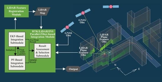
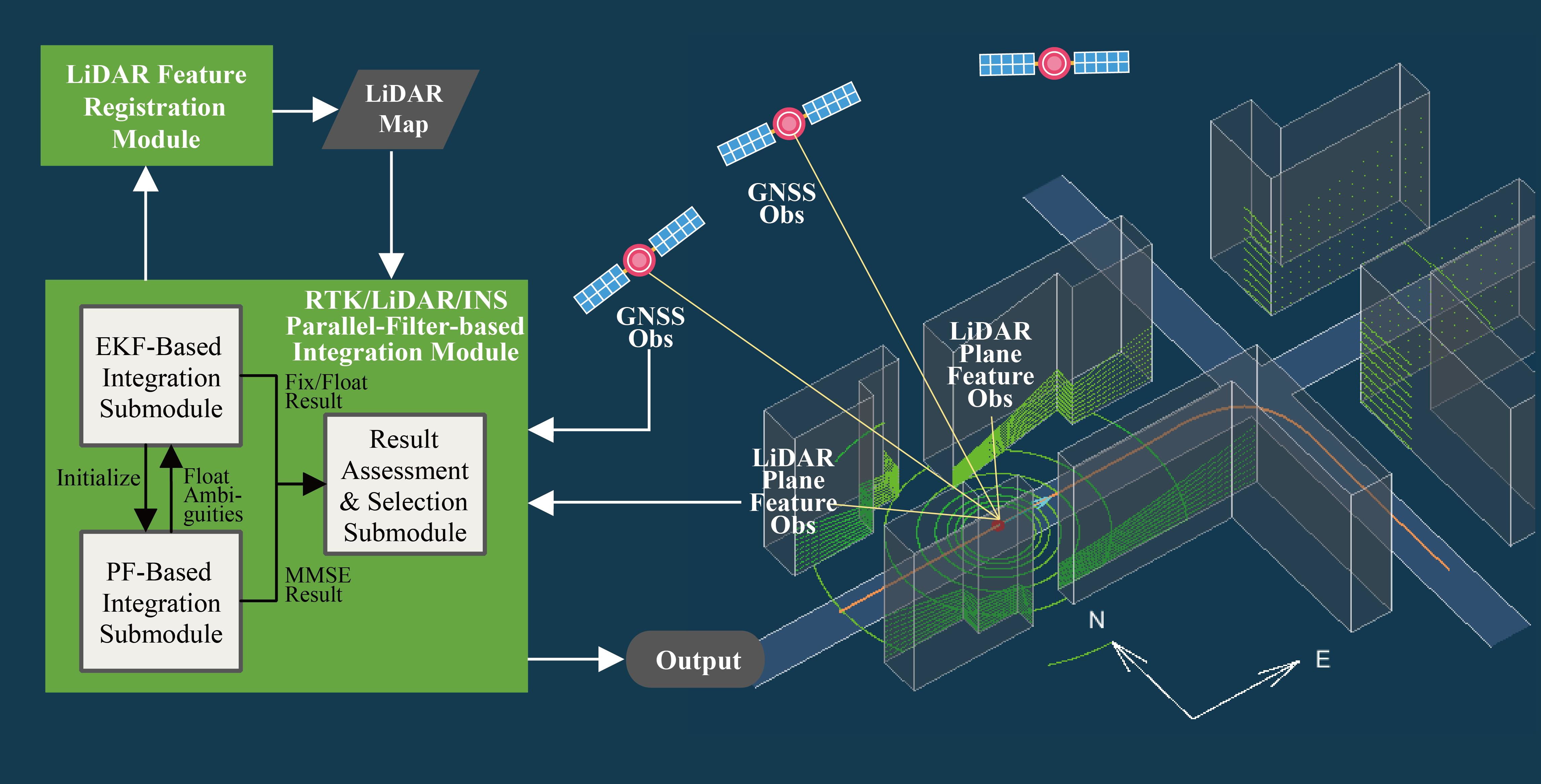
Figure 1 shows the general framework of our RTK/LiDAR/INS integrated system that consisted of four main modules, namely INS dead-reckoning module, LiDAR process module, RTK/LiDAR/INS parallel-filter-based integration module, and LiDAR feature registration module, respectively.
The core of the system was the RTK/LiDAR/INS parallel-filter-based integration module where an EKF-based algorithm in the ambiguity domain and a PF-based algorithm in the position domain were operated simultaneously. Both submodules integrated LiDAR features to RTK calculation and output positioning results, but aimed at different purposes. The main purpose of the PF-based integration submodule was to maintain the stability of the system. In this submodule, the PF with the MSR objective function was applied, which was insensitive to cycle slip and multipath effects on code pseudoranges, and the MMSE results were output to avoid instantaneous outliers. Since the PF has the problem of large samples, to lighten the burden of filtering, the PF state space lied in the positioning domain only, and thus, the task of estimating INS biases fell onto the EKF-based integration submodule. Moreover, the PF initial sample set was derived on the results of the EKF submodule. Meanwhile, the PF submodule returned the EKF module with more accurate MMSE float ambiguities after initialization. By doing so, the EKF-based algorithm can achieve a higher AR success rate and output higher precision positioning results with fixed integer ambiguities. Then, the MMSE positioning results and the fix/float positioning results of the two submodules were assessed and elected before the final output in the result assessment and selection submodule. The detailed procedure of this core module will be further addressed in
Section 4.
In the proposed system, the data output rate, sampling instant, and process complexity were different from sensor to sensor. Normally, the output rate of a multi-frequency GNSS receiver ranges from 1 to 10 Hz, while the ones of INS and LiDAR can reach up to 100 Hz and 10~20 Hz, respectively. The main task of the INS dead-reckoning module was to derive the state change between two GNSS epochs or within a LiDAR frame by means of accumulation and interpolation. Based on INS interpolation results, we can calibrate the distortion of the LiDAR point cloud that is caused by the scanning delay [
22]. For the calibrated point cloud, the Random Sample Consensus (RANSAC)-based plane extraction process [
23] was conducted, and the extracted plane feature measurements were then matched with the features pre-registered in the map.
Each GNSS epoch, we can utilize the current RTK result to update the global parameters of the LiDAR features in the LiDAR feature registration module, by which we realized a system of positioning while mapping.
3. Mathematical Models
The models of the sensors are normally established in their own coordinate frames, and when being integrated, involve issues such as coordinate system transformation. Therefore, before giving the equations of the models, we specify some scripts to indicate different coordinate frames, among which:
E represents the global frame, e.g., Earth-Centered Earth-Fixed (ECEF) or East-North-Up (ENU) coordinate;
B represents the body frame;
I represents the inertial frame;
L represents the LiDAR frame.
Here, we supposed that the INS frame was the same as the body frame and the transformation relationship between the body frame and LiDAR frame was rigorously calibrated in advance. Furthermore, the lever arm effects among the sensors were also well calibrated, so they were not considered in the following equations for description convenience.
In our RTK/LiDAR/INS integrated system, the observable landmarks included the moving GNSS satellites and the fixed LiDAR features and made up a diverse fusion map. The global coordinates of satellite landmarks can be derived from the broadcast ephemeris, so they were known quantities, while the ones of LiDAR landmarks were unknown without a prebuilt map. In contrast, for the observation of the landmarks, the ranges of GNSS carrier phases were ambiguous due to the unknown integer wavelength numbers, namely ambiguities, between the satellites and receiver, while the ones of LiDAR landmarks were accurate.
Therefore, the system measurement models can be divided into three parts, namely GNSS RTK, LiDAR, and INS, which are introduced below in sequence, and the parameters to be optimized included position, velocity, attitude, INS biases, ambiguities, and LiDAR landmark global parameters.
3.1. GNSS RTK Measurement Models
As for GNSS part, the distance measurements included pseudoranges and carrier phases. With the benefit of the GNSS receiver phase discriminator characteristics, the precision of carrier phases was much higher than the one of the pseudoranges, normally at the millimeter or centimeter level, and was less influenced by the multipath effect, thus making RTK a very high-precision positioning technology widely used in the surveying field. However, as mentioned previously, the ranges provided by carrier phase measurements were ambitious because only fractional phases and cycle counts from the initial acquisition can be achieved by the phase discriminators, which remain ambiguities to be estimated. Besides, both the pseudorange and carrier phase measurements contained many errors, which can be modeled as follows [
24]:
where
and
represent the pseudorange and carrier phase measurements between satellites
i and rover receiver
r, respectively,
represents the carrier phase wavelength,
represents the true geometric distance,
c represents the speed of light,
and
represent the receiver and satellite clock biases, respectively,
and
represent the tropospheric and ionospheric errors, respectively,
represents the ephemeris error,
represents the ambiguity,
and
represent the pseudorange and carrier phase multipath errors, respectively, and
and
represent the other errors that cannot be modeled.
RTK can eliminate most spatially related errors such as satellite clock errors, atmospheric errors, and ephemeris errors by differencing the measurements of rover
r and base
b and further eliminate the receiver clock errors by differencing between two satellites, forming the Double-Differenced (DD) measurement models as follows:
where
.
As we can infer from the above differencing, the positioning results that RTK provides were relative positions between a rover and a base station. Normally, the accurate absolute position of the base station was obtained in advance as a reference with which we can derive the global coordinates of the rover in real time accordingly.
3.2. LiDAR Plane Feature Measurement Models
As for the LiDAR part, the measurements that we employed were the parameters of the extracted features of the current point cloud in the LiDAR frame, and thus, the corresponding measurement models were the feature parameter transformation equations from the LiDAR frame to the global frame whose concrete expression depended on the feature types we used. The common geometric features included point, line, and plane features. In this paper, the system adopted the plane features that were easily found, extracted, and repeatedly observed in urban environments even with relatively sparse point clouds provided by 16-line 3D LiDARs. Generally, the plane feature is defined with the normal vector
n and the distance
d between the origin and the plane, and correspondingly, regardless of the measurement errors, the measurement model can be expressed as follows:
where
and
represent the parameters of plane
l in the LiDAR (L) and global (E) frames, respectively,
represents the user position in the global frame, and
represents the rotation matrix.
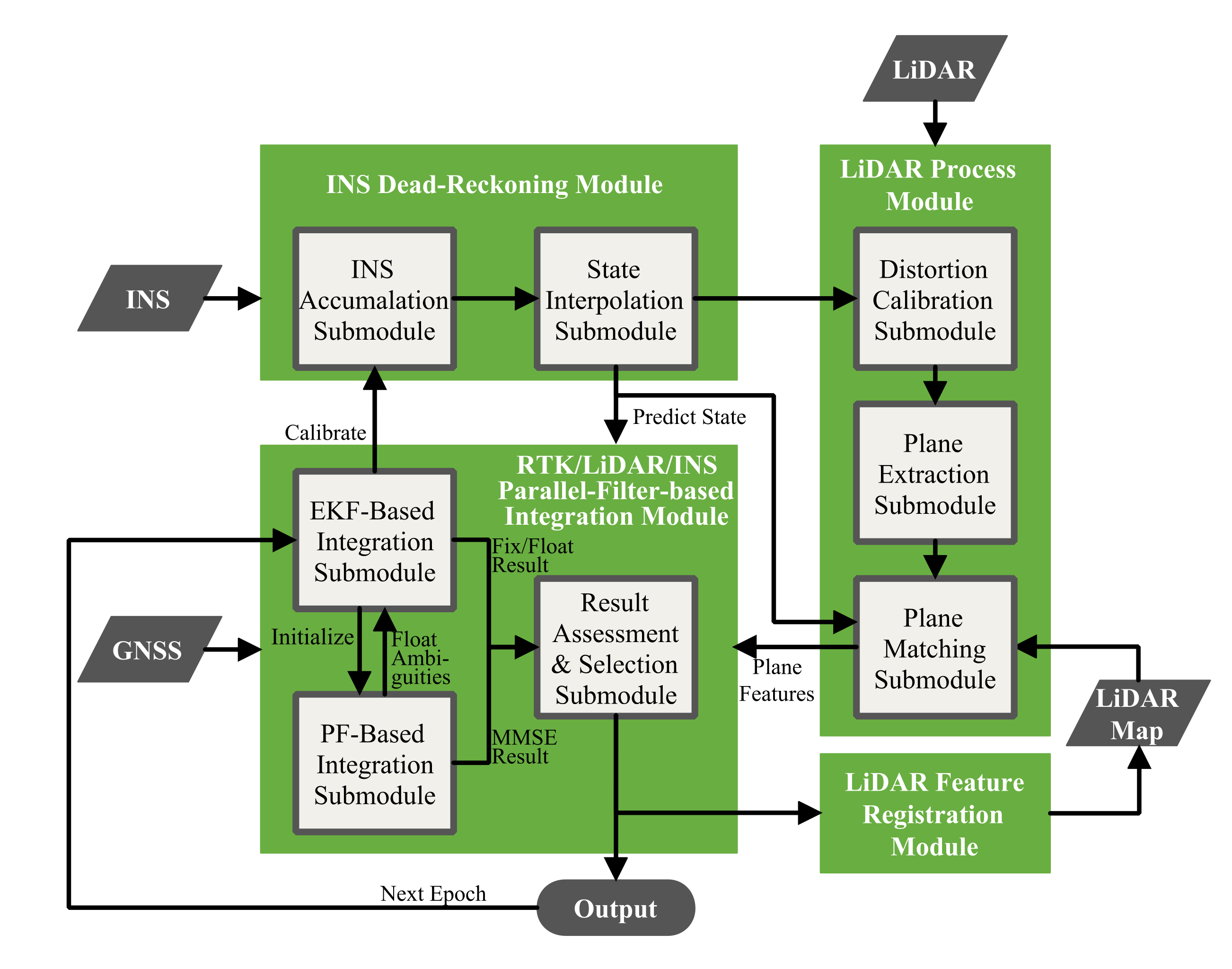
However, when being tightly coupled, due to the unit vector constraint of the normal vectors, it turns out to be uncontrollable when calculating the measurement residuals, filtering the states, or modeling the errors for the normal vectors. To settle the problem, we replaced the traditional plane parameters with a 3D point coordinate that was the foothold point of the origin to the plane, and it can be transformed from the original parameters form with
and used to identify a plane uniquely in a certain frame. The relationship between the footholds in the L frame and E frame is shown by
Figure 2.
We denote the foothold coordinates of plane
l in the LiDAR and global frames as
and
, respectively, and of note, these two coordinates point to two different points in space, of which the latter is fixed, while the former changes as the user position and attitude change. Then, according to the figure, the measurement models of the plane features can be derived as:
where
represents the LiDAR feature measurement noise vector.
3.3. INS Measurement Models
As a dead-reckoning sensor, the main duty of INS is to solve the precise interpolation and dynamic state prediction problems between two GNSS epochs. The INS measurement models consist of accelerometer and gyro outputs and can be modeled as [
25]:
where
and
represent the INS specific force and angular rate outputs, respectively,
and
represent the true values, respectively,
and
represent the biases of the accelerometer and gyro, respectively, and
and
represent other errors. The relationship between the true values of specific force and acceleration can be expressed as:
where
represents the acceleration true value and
represents the gravitational force.
3.4. System Total Measurement and State Transition Models
Above all, the total measurement equations can be concluded as:
where
represents the measurement noise, and the measurement vector is:
with:
where
M and
J represent the numbers of satellites and plane features, respectively, and
is the system state vector to be estimated with:
where
represents the velocity in the global frame,
represents the attitude, and
represents the DD ambiguity vector.
In our system, the process rate of the RTK/LiDAR/INS integrated positioning module was 1 Hz, and the position, velocity, and attitude variations between two consecutive epochs were derived from the INS accelerometer and gyroscope data accumulation. Thus, the total state transition equation can be modeled on the traditional INS state transition equations and added to the ambiguity equation, which is time-invariant if no cycle slip appears, as follows:
where
represents the system noise, and the detailed expression of
is:
where
represents the gravity vector in the global frame,
represents a zero matrix,
represents the skew symmetric matrix of angular velocity
:
and
,
,
where
and
represent the rotational angular rate of the Earth in the B frame and E frame, respectively.
4. Feature-Aided RTK/LiDAR/INS Integrated Positioning Algorithm with Parallel Filters in the Ambiguity-Position-Joint Domain
4.1. Basic Idea
Aiming at high-precision positioning in outdoor large-scale diversified environments without a prior map, we proposed an innovative RTK/LiDAR/INS integrated system. In the system, RTK was still used for sensor calibration and LiDAR mapping, but revolutionarily, tightly integrated LiDAR feature measurements to settle the problem of low satellite availability in GNSS-challenged areas. Besides, to further improve the RTK fix rate and the resistance of anomalies like cycle slips and large multipath errors on code pseudoranges, we adopted a parallel-filter scheme with ambiguity resolution in the ambiguity-position-joint domain.
Ambiguity Resolution (AR) is the key to RTK performance. According to the used search space, AR methods can fall into two categories, namely AR methods in the ambiguity domain and position domain, respectively. For the former, both filter and search are performed in the ambiguity space; the advantage is that the search space is relatively small, but the ambiguity filtering is easily disturbed by ambiguity changes caused by cycle slips. On the contrary, the AR methods in the position domain are insensitive to cycle slips, but subjected to large search space. Therefore, for these two kinds of methods, can we reserve the superiorities and make up the defects, for example, by combining them together?
Taking the above ideas into consideration, we proposed a feature-aided RTK/LiDAR/ INS integrated positioning algorithm with parallel filters in the ambiguity-position-joint domain. The basic structure of the algorithm is displayed in
Figure 1 as the core module, namely the RTK/LiDAR/INS parallel-filter-based integration module that consists of three submodules. The task assignment of these submodules is designed as follows:
The EKF-based integration submodule implements RTK/LiDAR/INS integrated positioning in the ambiguity domain, estimates all the states of the system, including INS accelerometer and gyroscope biases, and determines the initial search space for the PF method;
The PF-based integration submodule solves the AR problem in the position domain with the MSR objective function, outputs positioning results based on PF MMSE criterion, and gives reference float ambiguities as feedbacks to the EKF algorithm to revise its results in harsh situations;
Both revised EKF positioning results and PF MMSE positioning results are sent to the result assessment and selection submodule for output selection.
The detailed procedure of the algorithm is given as follows.
4.2. Preparation
Generally, for the initialization stage, the situation may not be challenging. For example, in an open area or static situation, RTK can achieve fix results easily in a stand-alone mode and be used for system and LiDAR feature map initialization. After the initialization, the state variation between two epochs can be predicted by the INS dead-reckoning results. Since the focus of our method was to improve the RTK performance by integrating with LiDAR measurements, both state prediction and LiDAR measurements should be synchronized to the GNSS observation epoch. Here, we denote the final output state vector of the last epoch
as
with:
and the position, velocity, and attitude variation derived by INS as
,
, and
, respectively. Then, the predicted stat of epoch
k can be obtained as:
The Random Sample Consensus (RANSAC) [
23] algorithm was adopted to extract plane features from the LiDAR point clouds, and the plane feature matching process was conducted subsequently. For the extracted plane
l with
, there is a plane in the LiDAR map, supposing plane
m with
, that satisfies the following condition:
where
represents the rotation matrix converted from
,
represents the threshold for plane matching, and
is regarded as the matched plane of
.
4.3. EKF-Based Integration in the Ambiguity Domain
The integration in the ambiguity domain was implemented based on the EKF, whose task is to provide the RTK fix results and estimate INS biases for calibration. The state space includes all state parameter to be estimated. The measurements included DD code pseudoranges, DD carrier phases, and LiDAR plane feature measurements. We denote the measurement vector at epoch
k as
:
The procedure of EKF-based RTK/LiDAR/INS integrated positioning in the ambiguity domain is given below.
The predicted state of epoch
k was derived with (
13), and the covariance matrix of the predicted state can be calculated with the following equation [
25]:
where
represents the time difference between two epochs,
represents the unit matrix,
represents the time interval,
represents the covariance matrix of state
at the last epoch,
represents the system noise covariance matrix, and
represents the state transition matrix whose expression is given as below:
where:
Then, we calculated the Kalman gain with the following equation [
26]:
where
represents the measurement noise covariance matrix and
represents the measurement matrix with the detailed form of:
where:
where
represents the unit Line Of Sight (LOS) vector from the receiver to satellite
i:
where
represents the global coordinate of satellite
i.
Next, we updated the state vector and its covariance matrix with the following equations:
where:
As mentioned previously, ambiguities have an integer constraint, but the ambiguity estimators of the EKF (
17) are float values. Therefore, the next step is the crucial part of RTK, namely AR, and the target is to search the optimal integer solution for the ambiguities. In this paper, the lambda method was adopted to solve the problem. As the most widely used AR method in RTK applications, lambda searches the optimal integer ambiguities within a given range in the ambiguity domain based on the following objective function [
27]:
where
is the covariance matrix of
obtained from (
18). The detailed procedure of the above optimum searching problem can be found in [
28].
After finding the optimal integer solution
, we can revise the user position with the equation as below:
and the corresponding covariance matrix can be derived as:
where
and
represent the covariance matrix of
and the correlation matrix between
and
obtained from (
18), respectively.
The integration of LiDAR features strengthened the geometric distribution, thus improving the RTK performance to some degree. However, in a real scenario, in addition to low satellite availability and a poor geometric distribution, frequent cycle slips and large multipath noises of code pseudoranges also bring challenges. With these challenges, the float ambiguities estimated by EKF could not converge rapidly, which means that might not be as accurate as we wanted.
To tackle the challenges of cycle slips and multipath effect, we designed a parallel submodule, which solves AR problem in the position domain and integrates carrier phase and LiDAR feature measurements only using the PF with a modified MSR objective function.
4.4. PF-Based Integration in the Position Domain
For the PF-based integration algorithm, two techniques play quite important roles in improving the robustness of the system. One is the MSR objective function that solves the AR problem in the position domain and is free of the effects of cycle slips and pseudorange multipath noises, and another one is the particle filter that further improves the stability of the outputs.
4.4.1. MSR Objective Function for the AR Problem
The MSR-based AR algorithm was proposed in [
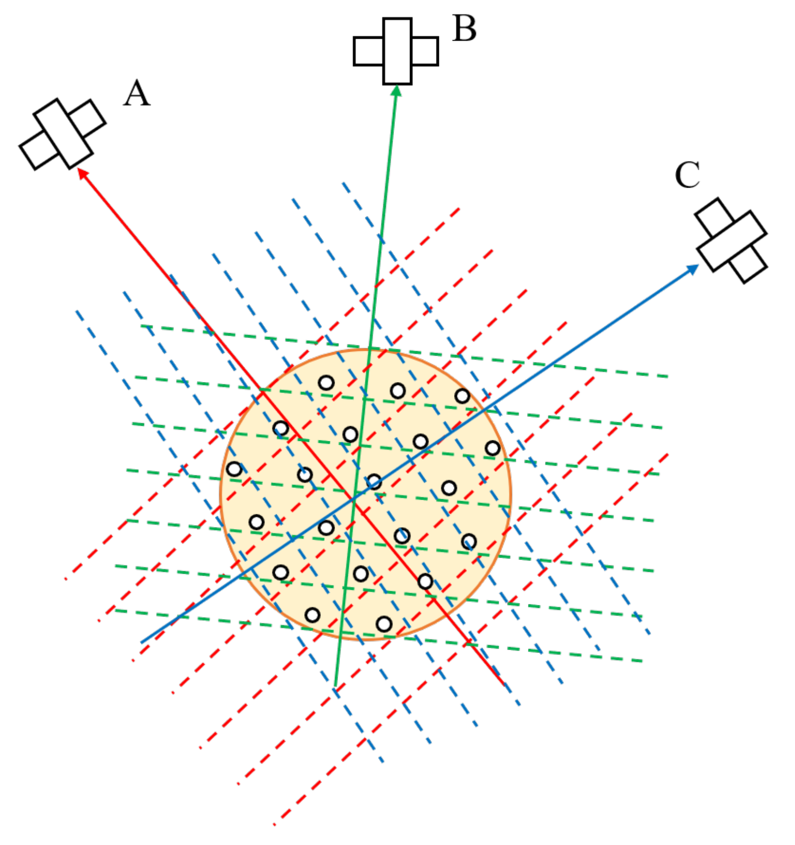
21]. The basic idea can be addressed briefly as follows. For a satellite, the carrier phase and its possible ambiguity can be related to a set of parallel surfaces, as shown by
Figure 3, which actually should be hyperboloids for DD measurements. If we ignore the existence of errors and noises, it can be found that an intersection point is located on one surface of each set, and this point is the true position we want. Although, due to noises, these surfaces may not intersect exactly at the same point; the true position is still quite near the surfaces corresponding to the correct ambiguities owing to the high-precision and multipath resistance characteristics of carrier phases. Therefore, the objective function that selects the best point from a set of position candidate points can be established by calculating the distance from the point to its nearest hyperboloids.
In details, for the candidate position point
, we used the following MSR objective function to determine whether it is the best point or not:
where
represents the carrier phase noise covariance matrix. The element of the distance vector
can be calculated by:
where
is the DD geometric distance derived by
with satellite
j and
k and
is the fractional function with the range from −0.5 to 0.5, and the corresponding DD ambiguity can be easily obtained by the following equation:
where
is the rounding function with the nearest integer.
Since the search space lies in the position domain, the method is insensitive to cycle slips. In addition, from above equations, we can see that the MSR is established on the strong integer constraint of the ambiguities, and the calculation involves carrier phase only, free of code pseudoranges with large multipath noises. Hence, compared with the traditional AR methods in the ambiguity domain, the method is more suitable for urban environments. The only remaining problem for the MSR-based AR method is how to select and manage the candidate position points, and in this paper, the PF was applied to handle the problem.
4.4.2. PF-Based Integration Algorithm
The basic idea of the PF is to approximate the state posterior probability distribution with a large number of sampling points, namely particles, in the state space by updating their weights iteratively [
29]. Since it is almost impossible to sample the posterior probability distribution directly, the PF introduces the concept of the importance sampling and samples another known probability distribution, namely the importance probability density function,
. Then, the state posterior probability distribution can be approximated with the weighted sum of these sampling points:
where
represents the state of epoch
k,
represents the measurements from Epoch 1 to
k,
represents the weight of particle
, and:
Here, in our PF-based integrated submodule, in order to reduce the complexity, we compressed the state space to the position state space, and further, to avoid the effect of large multipath errors in code pseudoranges, only carrier phases and LiDAR plane features were adopted as measurements in the PF calculation. Therefore, the state posterior probability distribution of our PF was
, and we denote the shrunken measurement vector of epoch
k as
with:
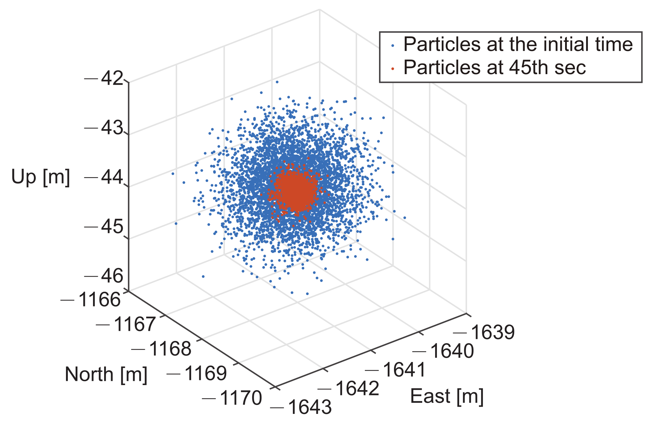
Supposing that we have an RTK fix positioning result that is derived by the EKF based submodule at epoch the center of initial sampling point set can be determined with , and the points are sampled based on a Gaussian distribution, , and assigned the same weights. Normally, for the initialization stage, the values of the covariance matrix should not be too small despite the high precision of . that is too small is not conducive to the approximation of the posterior probability density function in the position domain during the convergence process, especially in the situation where the initialization stage is a dynamic scene. Furthermore, considering both the error of the position state transition model and the situation where the particle filter may diverge when the observation condition deteriorates, the total number of particles should not be too small, either. Although the additional particles will increase the computational complexity of the algorithm, more particles can better guarantee the stability of the algorithm. That is, once the filter diverges, the filter can expand the position search space adaptively while maintaining a certain sampling density so that the true value can still stay within the search space and the algorithm is more likely to re-converge afterwards. In our method, we recommend and the number of sampling points NPF = 5000, both of which are the empirical values, but are sufficient for low dynamic scenes. We denote the particle set as and the weight of particle as .
Each epoch, we employed the state transition probability density function
as the importance probability density function to realize the importance sampling. In details, a new particle of epoch
k can be derived on the basis of the particle
of the last epoch with the following equation:
where
,
is the position variation derived by INS and
is the system noise covariance matrix of state
.
Then, we can update the weights of the particles with the following equation:
where
represents the measurement probability density function. By doing so, we not only integrate the measurements of carrier phases and LiDAR features, but also solve the AR problem with the aid of the MSR objective function in terms of probability.
The measurement probability density function that we used can be derived by the extensive form of the LiDAR-feature-integrated MSR objective function:
where
C is a coefficient whose value is inessential due to the subsequent weight normalization process, and the expression of the LiDAR-feature-integrated MSR objection function is given as below:
where
is the distance vector calculated with position
,
is the residual vector of LiDAR feature measurements based on the measurement model of (
7), and
is the LiDAR feature observation error covariance matrix, which is given in
Section 5.
Afterwards, the weights are normalized:
For the PF, there are several criteria for the output, such as Maximum A Posteriori (MAP) and the Minimum Mean-Squared Error (MMSE). In our method, for the sake of stability, we preferred MMSE criterion. Hence, the MMSE positioning result of the PF-based integration submodule can be calculated by:
Once the PF converges, we can feed back a more accurate referenced float ambiguity vector based on the MMSE to the EKF-based module to improve the fix rate of the AR method in the ambiguity domain by simply substituting the original float ambiguity vector with the following MMSE one in (
19):
Whether the MMSE float ambiguity vector converges to an acceptable accuracy depends on the indicator:
where
is the number of DD ambiguities.
Since the importance sampling has the problem of weight degeneracy, the resampling process is essential to the PF. That is, after a period of filtering, only a few particles have relatively large weights, while the weights of the rest are negligibly small. Therefore, we needed to resample the particles. Here, we adopted the resampling method of deleting the particles of small weights, copying the particles of large weights and setting all the new particles with the same weights.
4.5. Result Assessment and Selection
Each epoch, we can obtain three positioning results, namely the fix result and float result provided by the EKF-based submodule and the MMSE result provided by the PF-based submodule, respectively. As for , it can provide higher precision if the AR problem is correctly solved, but has the risk of wrong fixing, while for , the stability can be guaranteed at the sacrifice of a small precision loss, and the positioning precision can also be satisfactory after convergence. Therefore, the task of the result assessment and the selection submodule is to balance the precision and stability and pick one result for the final output.
The selection criterion can be defined at pleasure for different purposes. Here, as a reference, we provide one based on the classical AR ratio test [
30], predicted state, and the estimated accuracy of the MMSE result:
the submodule will output the fix result
and mark the status as fix one if the following conditions are both met:
where
is the suboptimum of the lambda method,
is the ratio threshold, and
is the estimated accuracy of the MMSE result:
if (
35) is not met, output the MMSE result
, and also, mark the status as fix one if the convergence condition is met:
if both (
35) and (
37) are not met, output the float result
, and mark the status as float one.
If an MMSE result is selected, the corresponding position covariance matrix can be approximated as:
where
is the diagonal matrix whose diagonal elements are composed of the elements of the vector.
Additionally, the final output result will be fed back to the EKF-based submodule and be used to predict the state of the next epoch.
5. LiDAR Feature Registration and Error Models
Once the final RTK result that we denote as
is obtained, we can use it to update the global parameters of the LiDAR feature landmarks with the following align:
It is worth noting that the accuracy of the above-calculated LiDAR global parameters is affected by the integrated factors such as RTK positioning errors, attitude errors, and LiDAR measurement errors. The existence of LiDAR global parameter errors suggests that the measurement models used in the subsequent observation epochs are inaccurate and are normally boiled down to model error. Therefore, we needed to take the errors of the global parameters into consideration when estimating the observation errors of the LiDAR features, which is similar to the situation of GNSS with regard to ephemeris errors.
Supposing that the position result, attitude result, and LiDAR measurements are irrelevant, with the use of:
where
represents the attitude error, and with the help of Taylor expansion, we can derive the covariance matrix of the LiDAR plane global parameter error based on (
39) as follows:
where
and
represent the covariance matrices of the RTK position and attitude results, respectively,
represents the internal measurement error covariance matrix of plane
j, and the expressions of the coefficient matrices are:
Then, for the subsequent epoch
t with the newly predicted user position
and rotation matrix
, if the global parameters of plane
j are derived at epoch
k, the observation error covariance matrix can be calculated by:
where
is the LiDAR feature internal error covariance matrix of epoch
t, and the coefficient matrix derived from the Taylor expansion of (
7) is given as below:
where
and
represent the predicted position and rotation matrix based on the predicted attitude
that is derived by INS at epoch
t, respectively.
The LiDAR feature internal error covariance matrix
depends on the working characteristic of the LiDAR itself. For LiDAR, the coordinate of a scanning point is derived with two direction angles and a ranging distance, which can be expressed as follows:
where
represents the ranging distance and
and
represent the horizontal and vertical angles, respectively. Therefore, the errors of the scanning points are affected by the ones of the direction angles and ranging distances. Since we adopted foothold coordinates to describe the plane features, even though the plane features are the extracted products of the point clouds, we still simply followed the model of the point errors whose covariance matrix, with the help of Taylor expansion, can be expressed below as a function of the direction angles and ranging distance:
where
and
represent the error amplitudes of the ranging distance and direction angles, respectively,
represents the normal vector with direction angles of
and
, and the expression of the coefficient matrix
is:
where
represents the distance from the origin to the plane.
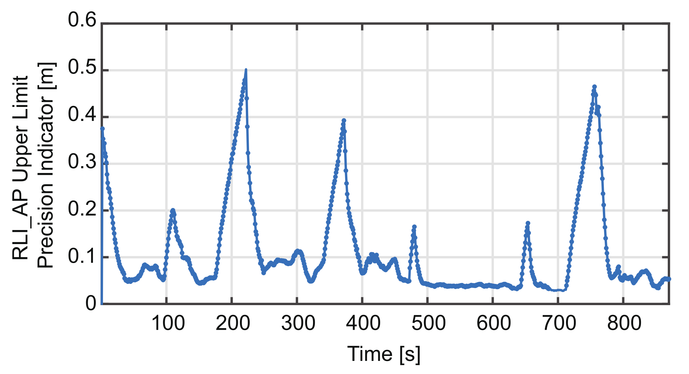
Since the update rate of integration was up to the one of GNSS data, which is normally 1 Hz, the update rate of mapping was also 1 Hz. Every epoch, we can calculate a new set of LiDAR global parameters based on the current RTK result and LiDAR measurements, and whether we substitute the old parameters of a certain landmark with new ones depends on whether the observation precision based on the new landmark parameters is higher. To be specific, the following precision indicator takes over the mission of assessing precision.
where
represents the sum of the diagonal elements and
is the re-calculated observation error covariance matrix at current epoch
k.
It is worth noting that the substitute criterion was based on the observation precision of (
41), not the global parameter precision of (
40), because what we cared about was how the global parameter precisions affect the integrated positioning rather than their actual values, which, in
Section 6, seemed to be “awful” owing to the far distance from the global frame origin to the plane.
6. Performance Theoretical Analyses
For the proposed RTK/LiDAR/INS integrated system, the aim was to improve RTK performance by integrating the measurements of LiDAR features and GNSS, as well as the parallel-filter scheme, and what we cared most about was whether or to what degree the RTK performance can be improved by these measures.
Therefore, in this section, we addressed several performance theoretical analyses and some simple simulations to validate our idea, which can be summarized as the following topics:
LiDAR plane feature global parameter and observation accuracies;
effect of the integration of LiDAR features on RTK AR success rate;
effect of parallel-filter scheme on RTK AR success rate;
effect of the integration of LiDAR features on RTK positioning accuracy.
In the following discussion, the epoch scripts are omitted from the equations for brevity.
6.1. LiDAR Plane Feature Global Parameter and Observation Accuracy Analysis
Since the observation accuracies of the LiDAR features have an impact on the integrated RTK while the global parameters of the LiDAR features are registered on the basis of the RTK results, we analyzed the precisions of LiDAR feature global parameters and the observation accuracies firstly.
The error models related to LiDAR features were addressed in
Section 5. In this section, we conducted several simple simulations as examples where the RTK position and attitude results were assumed to have been obtained already, as well as the variances or covariance matrices of the results, and the error amplitudes of the distances and direction angles of LiDAR plane features in (
42) were also given. Then, we designed a set of multiple unit normal vectors and simulated the global parameter accuracies based on (
40) and observation accuracies based on (
41) of the plane features with the designed unit normal vectors with different distances, successively, to analyze the accuracies in a direct-viewing way.
In the following simulations, the RTK positioning (latitude, longitude, height) and attitude results were set as (60
N, 120
E, 0 m) and (0, 0, 180
), respectively; the accuracies of the attitude results, LiDAR plane feature distances, and direction angles were set as,
, 0.02 m, and
, respectively; and the direction angles of the unit normal vectors in the L frame are listed in
Table 1. Among these vectors, the first four are the nearly horizontal ones that represent the features found in the UGV situation, while the last two represent the ones found in UAV situation. What is more, we designed two sets of parameters with different RTK positioning accuracies, namely 0.05 m and 0.3 m, respectively, the former of which represents the fix situation.
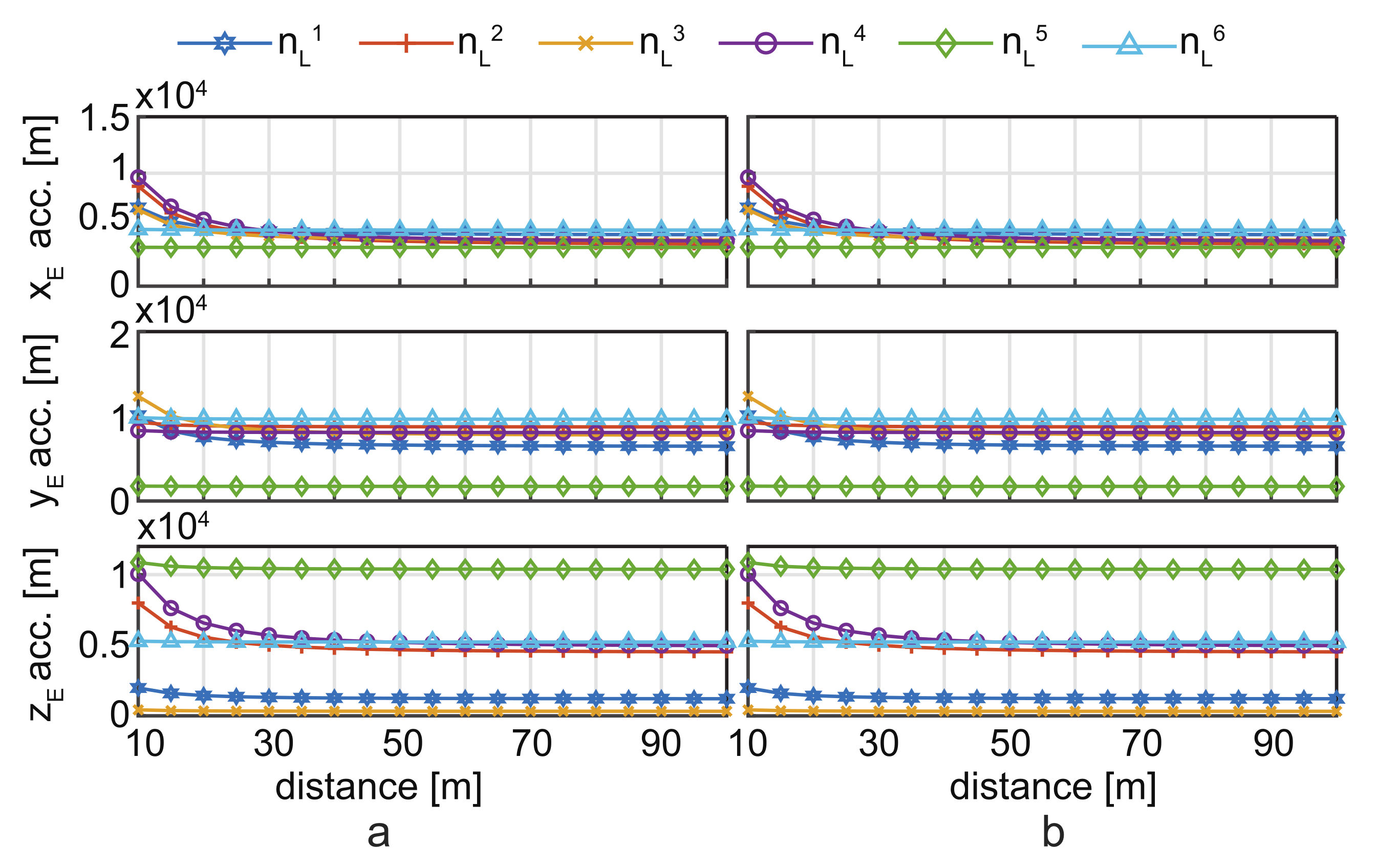
In the following simulations, we chose the ECEF coordinate as the global frame. The global parameter accuracy curves in three directions with ranging distances are shown in
Figure 4. From the figure, we can see that the accuracies of the global parameters look very “awful” no matter how precise the RTK positioning results were. Therefore, why are the global parameter accuracy we derived so large? From the expressions of
and
in (
40), we can find that, since the distance from the global frame origin to the user is much longer than the one from the user to the plane, the values of
and
become very large, which means that the errors of the global parameter calculated by (
40) are very sensitive to the attitude and LiDAR internal measurement errors. This phenomenon can also be explained from an intuitive point of view; that is, the origin of the global frame is much farther away from the planes compared with the user position, and thus, the tiny errors of the angles in local frame will be enlarged when we calculate a global foothold from a local one, which we call the distance effect. Moreover, the larger the ratio between the distance from the global origin to the plane and the one from the user position is, the greater the impact of angle errors may have on the LiDAR global parameter accuracy, which can be evidenced in our simulation with the phenomenon: as the observation distance increases, instead of increasing, the curves of the global parameter errors present a descending trend.
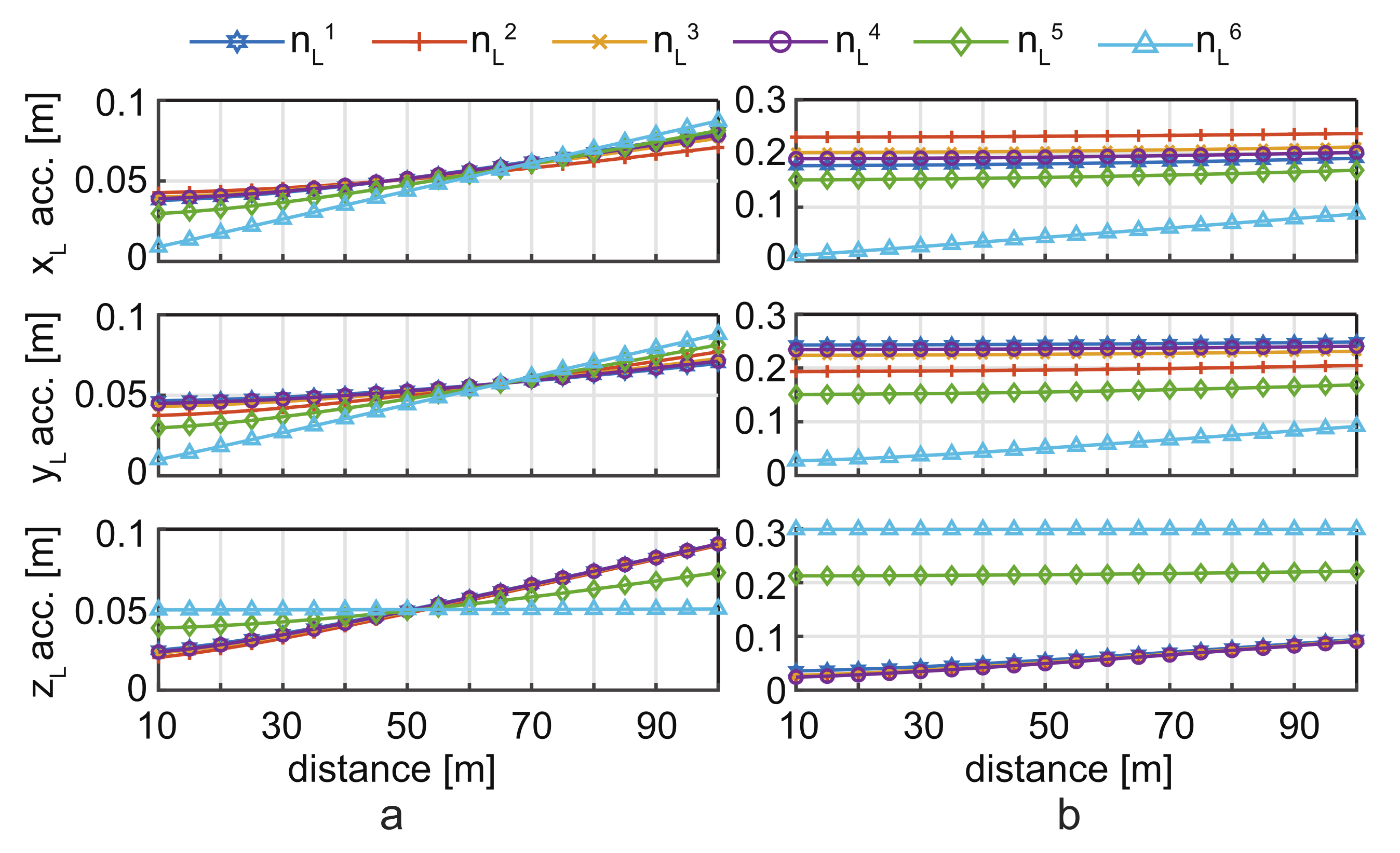
Then, can we still use these global parameters with such “bad” accuracy in our integrated positioning algorithm? The answer is yes. In fact, although the global parameter errors are quite large, due to the same reason as the distance effect, when calculating the observation errors that consider the global parameter errors, namely Equation (
41), the effect of the global parameter errors is greatly weakened.
Figure 5 displays the observation errors based on the above global parameter errors at the same observation spot. As we can see from the figure, with high-precision RTK fix positioning results, the observation errors in each direction were less than 0.1 m within a 100 m observation distance range, and the observation errors were also acceptable with the 0.3 m positioning accuracy, which suggests that the observation accuracy of the LiDAR plane features with global parameters based on RTK results was quite high and, thus, usable for RTK integrated calculation. Moreover, the plane observation errors were shown to be proportional to the observation distance, which accorded with the intuitive sense for LiDAR observation.
6.2. Effect of the Integration of LiDAR Features on the RTK AR Success Rate
From the above simulation, we know that, after deriving the global parameters based on RTK results, the observation accuracy of LiDAR plane features is lower than that of carrier phases, but equivalent to or even higher than that of pseudoranges. Therefore, to what degree can LiDAR feature integration improve the performance of RTK? As the most crucial indicator for RTK performance, the RTK AR success rate was analyzed here. To be specific, we adopted the following Ambiguity Dilution of Precision (ADOP)-based AR success rate estimation equation to assess the improvement [
31]:
where
represents the Gaussian cumulative distribution function and:
where
M represents the number of the satellites,
represents the covariance matrix of the float ambiguities, and
represents the determinant function. From the above equations, we can discover that the AR success rate is a function of the float ambiguity covariance matrix, and thus, we derived the change in
after integrating with LiDAR features. Here, to facilitate derivation and analysis, we made the following assumptions to simplify the model:
Assumption 1. Assuming that the measurement errors follow the Gaussian distribution and the corresponding covariance matrices are irrelevant to the estimators, then the Cramer–Rao Lower Bound (CRLB) of the estimators can be obtained as follows: Assumption 2. We assumed that the measurement error covariance matrix can be simply expressed as the product of the error coefficients and the proportional matrices, that is,where,, andrepresent the measurement error covariance matrices of pseudoranges, carrier phases, and LiDAR plane features, respectively. Then, we can derive the CRLBs of the float ambiguities with and without LiDAR integration, which are given as below:
Without LiDAR integration:
Since , before being tightly integrated with LiDAR features, the accuracy of the float ambiguities is mainly dominated by the one of the pseudoranges. After the integration, the influences of the pseudorange errors are weakened by the added term of , and thus, the float ambiguity accuracy is greatly improved, as well as the RTK AR success rate.
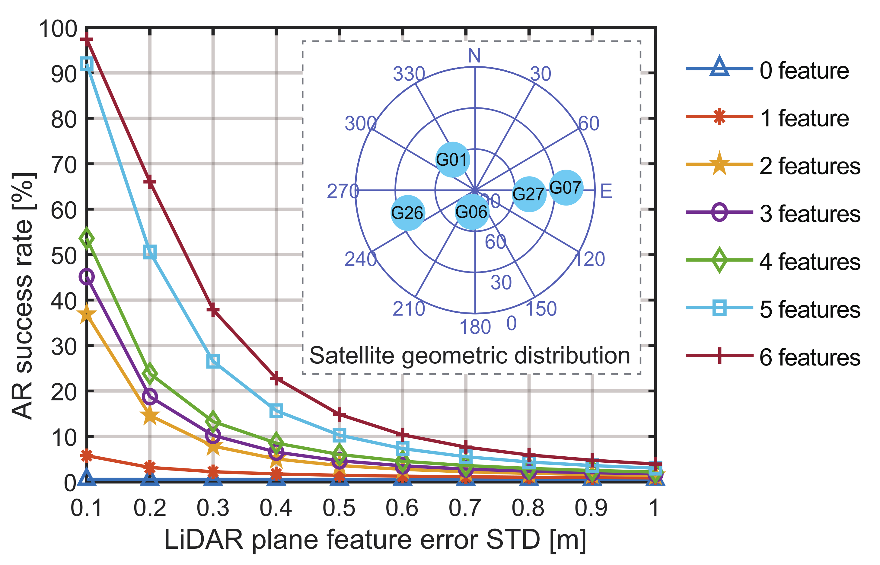
Here, we also conducted a simulation with the scenario of an urban canyon and the GNSS noises slightly larger than those in open areas to evaluate the improvement of the RTK AR success rate after integrating with different numbers of LiDAR features of different observation accuracies. The simulation satellite geometric distribution is given in the dashed box of
Figure 6, where, due to the blockage, almost all the satellites were located in the east-west direction, and the GNSS pseudorange and carrier phase noise coefficients
and
were set as 0.5 m and 0.005 m, respectively. The normal vectors used in the simulation were the same as the ones in
Table 1.
Figure 6 gives the AR success rates with a different number of features and LiDAR measurement error Standard Deviations (STDs).
As shown in the figure, in the GNSS-challenged environment we set, RTK can hardly solve the AR problem in a stand-alone mode. As the number of LiDAR features increased, the AR success rate increased, and the higher the LiDAR observation accuracy was, the higher AR success rate we could achieve.
6.3. Effect of the Parallel-Filter Scheme on the RTK AR Success Rate
Here, a qualitative analysis was performed for the RTK AR success rate of the parallel-filter scheme.
In our parallel-filter framework, the PF-based submodule provides a referenced MMSE float ambiguity vector
to the EKF-based submodule whose accuracy is accountable for the AR success rate. Although it is hard to obtain the covariance matrix with PF, we can use the following equation to approximate the covariance matrix of
:
which actually reflects the convergence state of the PF.
As introduced previously, the state space of our PF lies in the position domain only, and the weight update process involves carrier phases and LiDAR features only, which protects the filtering process from the effects of cycle slips and code multipath noises. Once the PF converges, the accuracy of is guaranteed, as is the AR success rate.
6.4. Effect of the Integration of LiDAR Features on RTK Positioning Accuracy
In addition, we derived the influence of LiDAR integration on the RTK positioning results. Since the accuracies of the RTK fix and float results had large difference, we derived the CRLBs for both types of results. As for the accuracy of the MMSE positioning results, it depends on the convergence status of the filter whose evaluation equation was already addressed with (
36), and thus, we do not discuss it in the following part.
In detail, without LiDAR integration:
From the above equations, we can see that, before integration, the RTK float positioning accuracy was mainly dominated by the pseudorange accuracy, while the fix positioning accuracy mainly depended on the carrier phase accuracy. After integration, since , the integration of LiDAR features contributed more to the float results, while having little influence on the fix ones, which were still dominated by the carrier phase accuracy.
Most importantly, matrix represents the geometric distribution of the LiDAR features, which means that the LiDAR feature distribution also had something to do with the positioning results. Normally, in the direction where satellite signals are blocked, shelters such as buildings exist, which indicates that there is a high probability for us to extract LiDAR plane features from that direction to make up the geometric distribution of GNSS satellites, thus improving the positioning accuracy in the occlusion direction.
8. Conclusions
To realize high-precision positioning in outdoor large-scale diversified environments without a prior map, we addressed a new RTK/LiDAR/INS integrated positioning algorithm. Since we still counted on RTK for maintaining the global positioning precision of the integrated system, the main focus of the proposed algorithm was to improve the performance of RTK in GNSS-challenged environments with the aid of other sensors and a robust AR scheme. With this purpose in mind, we further explored the idea of our previous work, which utilized RTK results to register LiDAR features while integrating the measurements of the pre-registered LiDAR features with RTK. Specifically, we upgraded the method by using innovative parallel filters in the ambiguity-position-joint domain to further weaken the effects of low satellite availability, cycle slips, and multipath effects.
The theoretical analyses, simulation, and road test experiment results indicated that the proposed method improved the RTK fix rate and output stability in GNSS-challenged environments and, thus, guaranteed the whole system with more stable and high-precision global positioning results in outdoor diversified environments. However, as the price of the performance improvement, the proposed method required more calculation time owing to the LiDAR data processing and particle filter and caused delays in RTK result output. Therefore, the method is more recommended for low-speed applications or to be used in a delay-tolerant background as a measure for maintaining the global precision of the whole system.
For a robust positioning system, fault detection and exclusion algorithms are also of great importance, among which Receiver Autonomous Integrity Monitoring (RAIM) offers the most rigorous implementation framework. Therefore, for our future work, the proposed RTK/LiDAR/INS integrated positioning system with fault detection and exclusion based on the RAIM framework will be studied and tested.


